Integration of the vegetation phenology module improves ecohydrological simulation by the SWAT-Carbon model

Vegetation phenology and hydrological cycles closely interact from leaf and species levels to watershed and global scales. As one of the most sensitive biological indicators of climate change, vegetation phenology is essential to be simulated accurately in hydrological models. Although the Soil and Water Assessment Tool (SWAT) has been widely used for estimating hydrological cycles, its lack of integration with the phenology module has led to substantial uncertainties. In this study, we developed a process-based vegetation phenology module and coupled it with the SWAT-Carbon model to investigate the effects of vegetation dynamics on runoff in the upper reaches of the Jinsha River watershed in China. The modified SWAT-Carbon model showed reasonable performance in phenology simulation, with root mean square error (RMSE) of 9.89 d for the start of season (SOS) and 7.51 d for the end of season (EOS). Simulations of both vegetation dynamics and runoff were also substantially improved compared to the original model. Specifically, the simulation of leaf area index significantly improved with the coefficient of determination (R²) increasing by 0.62, the Nash–Sutcliffe efficiency (NSE) increasing by 2.45, and the absolute percent bias (PBIAS) decreasing by 69.0 % on average. Additionally, daily runoff simulation also showed notable improvement, particularly in June and October, with R² rising by 0.22 and NSE rising by 0.43 on average. Our findings highlight the importance of integrating vegetation phenology into hydrological models to enhance modeling performance.

1 Introduction

Vegetation plays a crucial role as a link between the land and the atmosphere through its influence on carbon, water, and energy cycles (Bonan, 2008; Zhou et al., 2023). Vegetation phenology is one of the most sensitive bioindicators of climate change (Fu et al., 2015; IPCC, 2021; Vitasse et al., 2022) and closely interacts with the hydrological cycles (Hwang et al., 2014; Kim et al., 2018; Chen et al., 2022a). Therefore, vegetation phenological processes must be accurately simulated in hydrological models. The Soil and Water Assessment Tool (SWAT) has been widely used to model hydrological processes in watersheds (Bhatta et al., 2019; Tian et al., 2020). However, the performance of its vegetation module and its simulation of vegetation phenology remain poor, resulting in large uncertainties in the simulation of hydrological processes (Chen et al., 2023). To improve projections of ecohydrological processes under future climate change conditions, it is essential to modify the vegetation module by considering vegetation phenology.

In recent decades, climate change has substantially shifted vegetation phenology, with an advance in the start of season (SOS) (Fu et al., 2014) and a delay in the end of season (EOS) (Piao et al., 2019). This has extended the growing season by 2–10 d per decade (Zhao et al., 2015; Garonna et al., 2016; Shen et al., 2022), closely interacting with hydrological processes from leaf and species levels to watershed and global scales (Chen et al., 2022b). At the leaf scale, earlier spring leaf-out would enhance transpiration and increase the water requirement of plants, resulting in greater water flux from the soil to the atmosphere. At the watershed scale, the extension of the vegetation growing season would reduce runoff through increased evapotranspiration (ET) (Kim et al., 2018; Gaertner et al., 2019; Geng et al., 2020). Shifts in vegetation phenology affect both the magnitude and the timing of hydrological processes (Creed et al., 2015; Hwang et al., 2023). Therefore, developing a hydrological model capable of characterizing vegetation phenology is essential for a comprehensive understanding of hydrological processes.

The SWAT model has been extensively used to assess the impact of climate change on hydrological processes across a variety of watershed scales. The updated SWAT-Carbon model was developed to enhance the simulation of terrestrial carbon and water cycles (Zhang et al., 2013; Mukundan et al., 2023). Like SWAT, SWAT-Carbon employs a simplified version of the Environmental Policy Impact Climate (EPIC) vegetation growth module (Arnold et al., 1998), which determines SOS and EOS based on a day-length threshold calculated as a function of latitude. However, phenological processes are complex, determined not only by day length but also by temperature and precipitation (Peñuelas et al., 2004; Piao et al., 2015; Wu et al., 2021). For example, temperature is regarded as the dominant driver of spring phenology, with spring warming largely advancing leaf-out dates by meeting the forcing requirement earlier (Ge et al., 2015; Fu et al., 2018). However, winter-warming-induced reductions in chilling accumulation would increase the forcing requirement and delay the leaf-out dates (Fu et al., 2015; Wu et al., 2023). Therefore, the EPIC module fails to capture the actual phenological processes (Ma et al., 2019), making it urgent to couple a specific phenology module with the SWAT-Carbon model to simulate hydrological processes accurately.

The upper reaches of the Jinsha River watershed, originating from the Tibetan Plateau and forming the upper reach of the Yangtze River, are recognized as one of the ecologically fragile regions in China. In recent years, the upper reaches of the Jinsha River watershed experienced significant climate change, greatly influencing vegetation dynamics and regional water cycles (Wu et al., 2020; Li et al., 2022; Jiang et al., 2024). Enhancing our understanding and simulation of ecohydrological processes in the upper reaches of the Jinsha River watershed is critical for securing water resources and maintaining ecological stability. In this study, we first developed a process-based vegetation phenology module for the upper reaches of the Jinsha River watershed, which consists of spring and autumn phenology models that consider both temperature and photoperiod. Subsequently, we coupled this module with the SWAT-Carbon model. The objectives of our study are as follows: (1) to develop a process-based vegetation phenology module and integrate it into the SWAT-Carbon model; (2) to elucidate the effects of vegetation phenology and climate change on watershed ecohydrological processes; and (3) to forecast future shifts in runoff under different emission scenarios using the modified SWAT-Carbon model.

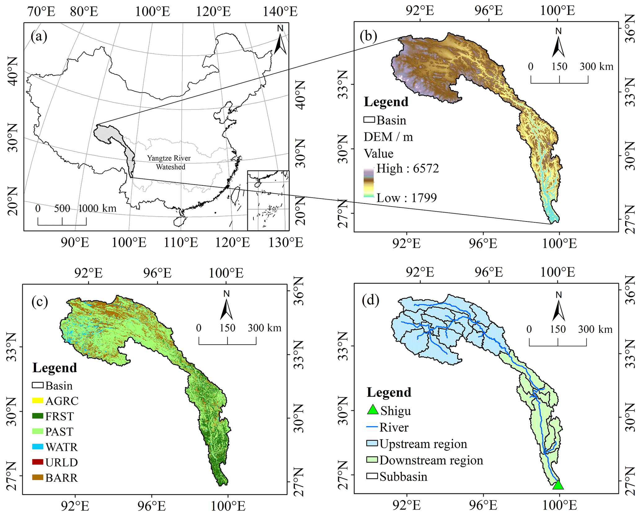
Figure 1 Study area. Location of the upper Jinsha River watershed (a), digital elevation model (DEM) (b), distribution of land use types (c) (AGRC – farmland; FRST – forest; PAST – grassland; WATR – water; URLD – residential area; BARR – unused land), and division of subbasins and the location of the Shigu hydrological gauging station (d).

2 Materials and methods

2.1 Study area

Our study focused on the upper reaches of the Jinsha River watershed in China, located in the upper reach of the Yangtze River (Fig. 1a). The elevation difference of the upper Jinsha River watershed is 4773 m (Fig. 1b), and the drainage area covers 216 440 km². The multiyear mean temperature was approximately −2.56 ± 4.11°C, and the multiyear mean annual precipitation was approximately 467 ± 135 mm from 1982 to 2018. Influenced by monsoons, precipitation is mainly observed during June–September, accounting for over 75 % of the annual total, with the highest monthly precipitation typically recorded in July. The land use types in the study area changed little during 2007–2014, with grassland (61.4 %) and forest (14.6 %) representing the dominant vegetation types (Fig. 1c). Grassland areas are primarily distributed in the upstream region of the basin, whereas forests are prevalent in the downstream area.

Table 1 Details of the data used in this study.

2.2 Dataset

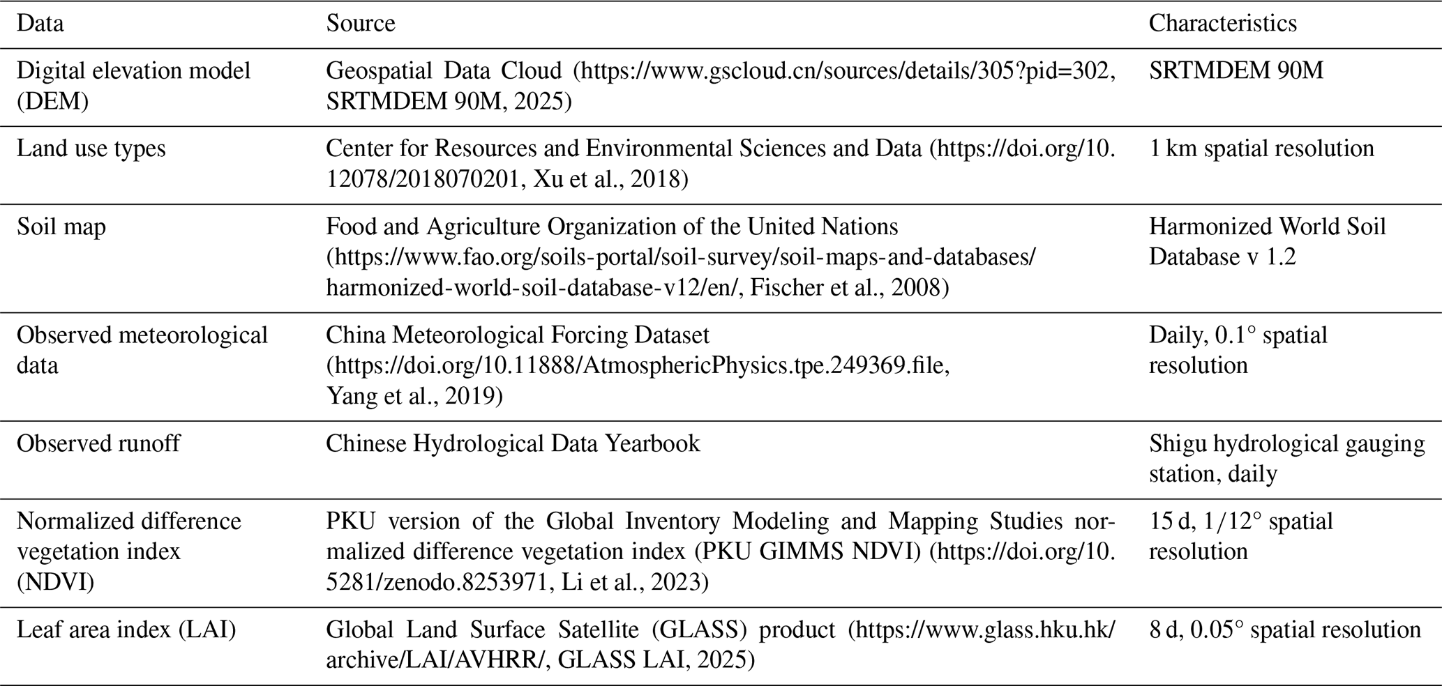
The sources of the datasets used for phenology models and the SWAT-Carbon model are listed in Table 1.

2.2.1 Digital elevation model (DEM), land use, and soil data

The watershed and river network of the study area were delineated using a digital elevation model (DEM) with 90 m resolution (Fig. 1b) in ArcSWAT2012 (https://swat.tamu.edu/, last access: 10 April 2025). The watershed was first subdivided into 28 subbasins (Fig. 1d) based on topographic characteristics and then discretized into 1922 hydrologic response units (HRUs) based on land use, soil data, and slope characteristics.

We extracted land use data with 1 km spatial resolution from the Resources and Environmental Sciences and Data Center, Institute of Geographic Sciences and Natural Resources Research, Chinese Academy of Sciences (Xu et al., 2018). These data were reclassified to match the land use classes for HRU delineation in the SWAT-Carbon model (Fig. 1c). There were six classes of land use identified in the watershed: farmland (AGRC), forest (FRST), grassland (PAST), water (WATR), residential area (URLD), and unused land (BARR).

The soil map of the upper reaches of the Jinsha River watershed was obtained from the Food and Agriculture Organization of the United Nations (Fischer et al., 2008). We used the Soil–Plant–Air–Water model (SPAW; https://www.ars.usda.gov/research/software/, last access: 10 April 2025) to develop the database of soil properties for the watershed.

2.2.2 Climate data and runoff

Gridded climate data were processed as observed values to force both the original and the modified SWAT-Carbon models, in consideration of the limited distribution of meteorological stations. We used daily meteorological data from 1982 to 2018 with 0.1° spatial resolution, extracted from the China Meteorological Forcing Dataset (CMFD), which included precipitation, temperature, relative humidity, wind speed, and solar radiation (He et al., 2020). This dataset was developed by the Institute of Tibetan Plateau Research under the Chinese Academy of Sciences, and it represents the optimal combination of in situ observations, satellite retrievals, and meteorological reanalysis.

Coupled Model Intercomparison Project Phase 6 (CMIP6) outputs were used to predict vegetation phenology and future runoff. We selected four CMIP6 models, i.e., CanESM5, FGOALS-g3, MPI-ESM1-2-HR, and MRI-ESM2-0, which were commonly used in studies of the Yangtze River (Zhang et al., 2023; He et al., 2024). The daily time series of mean temperature, maximum temperature, minimum temperature, and precipitation under three emission scenarios (Shared Socioeconomic Pathway (SSP) SSP1-2.6, SSP2-4.5, and SSP5-8.5) were acquired from the CMIP6 website (https://esgf-node.llnl.gov/search/cmip6/, last access: 10 April 2025). CMIP6 data are biased in local areas (Stevens and Bony, 2013), making it necessary to correct these errors. First, we interpolated the CMIP6 data to 0.1° spatial resolution using linear interpolation. Then, the CMFD was employed as the reference to correct the bias in CMIP6 models using the empirical mapping technique (Gudmundsson et al., 2012; Wilcke et al., 2013). Daily empirical cumulative distribution functions for the calibration period were produced using a moving window of ± 15 d (Thrasher et al., 2012).

Daily runoff data (2007–2014) of the Shigu hydrological gauging station, located at the upper reaches of the Jinsha River watershed outlet, were obtained from the Chinese Hydrological Data Yearbook.

2.2.3 Vegetation data

We obtained the PKU version of the Global Inventory Modeling and Mapping Studies normalized difference vegetation index (PKU GIMMS NDVI) dataset (https://doi.org/10.5281/zenodo.8253971, Li et al., 2023) for 1982–2022 (spatial resolution: $\mathrm{1}/\mathrm{12}$°; temporal resolution: every 15 d).

Leaf area index (LAI) data from 1982 to 2018 were acquired from the Global Land Surface Satellite (GLASS) product with 0.05° spatial resolution and an 8 d temporal interval (https://www.glass.hku.hk/archive/LAI/AVHRR/, GLASS LAI, 2025). LAI time series for forest and grassland areas were obtained through area-weighted averaging of FRST and PAST grid values within the studied watershed (Strauch and Volk, 2013; Zhang et al., 2020).

2.3 SWAT-Carbon model modification

The SWAT model is a comprehensive, process-oriented, and physically based semi-distributed hydrological model (Neitsch et al., 2011). The SWAT-Carbon model (https://sites.google.com/view/swat-carbon/home, last access: 10 April 2025), as an updated version, has been developed to enhance the simulation of terrestrial carbon cycles. However, the SWAT-Carbon model still performs poorly in estimating vegetation dynamics (e.g., phenology and LAI). The current SWAT-Carbon model uses day-length thresholds that are determined only by latitude to simulate the onset and the end of vegetation dormancy. This approach fails to accurately capture vegetation dynamics as it largely ignores the effects of other important environmental factors (i.e., temperature) (Chen et al., 2023). Incorporating accurate phenology information could enhance the simulation of LAI, thereby improving the accuracy of runoff simulated by the hydrological model. The UniChill model and the DM model, which account for the response of phenology to various environmental variations, have been widely used to simulate spring and autumn phenology (Yang et al., 2012; Roberts et al., 2015). Therefore, we modified the SWAT-Carbon model by integrating the process-based vegetation phenology module. This phenology module consists of two phenology models: the UniChill model for simulating SOS and the DM model for simulating EOS. These phenology models provide dynamic simulations of vegetation phenology to replace the fixed dates of the SOS and EOS in the SWAT-Carbon model without the need for adjusting management operations. Subsequently, we set the heat accumulation calculated between dynamic phenology dates, instead of the default constant, as the annual heat requirement for vegetation growth. This dynamic heat requirement was then used to calculate daily variations in LAI.

The UniChill model, proposed by Chuine (2000), hypothesizes that spring phenology is regulated both by chilling temperatures and forcing temperatures during the dormancy period. Because of the specific range of chilling and forcing temperatures, we added temperature conditions when calculating the state of the chilling and forcing phases (Fu et al., 2012). The chilling phase starts at the onset of dormancy (t₀, fixed to 1 September) and is active on days with mean temperature between −5 and 10°C. The rate of chilling (R_C) can be expressed as follows.

$$\begin{array}{}\text{(1)}& R_{\mathrm{C}}=\left\{\begin{array}{ll}\frac{\mathrm{1}}{\mathrm{1}+{\mathrm{e}}^{C_{\mathrm{a}}(x-C_{\mathrm{c}}{)}^{\mathrm{2}}+C_{\mathrm{b}}(x-C_{\mathrm{c}})}}& \text{if }-\mathrm{5}\le x\le \mathrm{10}\\ \mathrm{0}& \text{if }x>\mathrm{10}\text{ or }x<-\mathrm{5}\end{array}\right.\end{array}$$

Here x is the daily mean air temperature, and C_a, C_b, and C_c are chilling rate parameters.

The chilling phase ends with the onset of quiescence (t₁), which occurs when the state of chilling (S_C; Eq. 2) reaches the critical state of chilling (Eq. 3).

$$\begin{array}{}\text{(2)}& {\displaystyle }& {\displaystyle }{S}_{\mathrm{C}}=\sum _{t_{\mathrm{0}}}^t{R}_{\mathrm{C}}\left(x_t\right)\text{(3)}& {\displaystyle }& {\displaystyle }t=t_{\mathrm{1}}\text{ if }{S}_{\mathrm{C}}>C^{\ast }\end{array}$$

The forcing phase begins at t₁ and is active on days with mean temperature above 0°C.

$$\begin{array}{}\text{(4)}& R_{\mathrm{F}}=\left\{\begin{array}{ll}\frac{\mathrm{1}}{\mathrm{1}+{\mathrm{e}}^{F_{\mathrm{b}}(x-F_{\mathrm{c}})}}& \text{if }x>\mathrm{0}\\ \mathrm{0}& \text{if }x\le \mathrm{0}\end{array}\right.\end{array}$$

Here F_b and F_c are forcing rate parameters.

The forcing phase ends with the occurrence of SOS (t₂), which occurs when the state of forcing (S_F; Eq. 5) reaches the critical state of forcing (Eq. 6).

$$\begin{array}{}\text{(5)}& {\displaystyle }& {\displaystyle }{S}_{\mathrm{F}}=\sum _{t_{\mathrm{1}}}^t{R}_{\mathrm{F}}\left(x_t\right)\text{(6)}& {\displaystyle }& {\displaystyle }t=t_{\mathrm{2}}\text{ if }{S}_{\mathrm{F}}>F^{\ast }\end{array}$$

The DM model (Delpierre et al., 2009) is based on the assumption that leaf senescence is driven both by the photoperiod and low temperatures. This model represents the progress of senescence processes using a coloring state (S_sen) for each day (d), which is the accumulation of the daily rate of senescence (R_sen). Senescence starts on the date (D_start) when the photoperiod is shorter than a specific threshold (P_start), and the EOS is recognized as when S_sen exceeds the threshold value Y_crit. The functions expressed in the process are as follows.

$$\begin{array}{}\text{(7)}& {\displaystyle }\mathrm{\text{if }}P\left(d\right)<P_{\text{start}}\left\{\begin{array}{ll}\text{if }T\left(d\right)<T_{\mathrm{b}}& R_{\text{sen}}\left(d\right)=[T_{\mathrm{b}}-T(d){]}^x\\ & \times f\left[P\right(d){]}^y\\ \text{if }T\left(d\right)\ge T_{\mathrm{b}}& R_{\text{sen}}\left(d\right)=\mathrm{0}\end{array}\right.\text{(8)}& {\displaystyle }\text{if }\left\{\begin{array}{ll}P\left(d\right)\ge P_{\text{start}}& S_{\text{sen}}\left(d\right)=\mathrm{0}\\ P\left(d\right)<P_{\text{start}}& S_{\text{sen}}\left(d\right)=S_{\text{sen}}(d-\mathrm{1})+R_{\text{sen}}\left(d\right)\end{array}\right.\text{(9)}& {\displaystyle }f\left[P\right(d\left)\right]={\displaystyle \frac{P\left(d\right)}{P_{strat}}}\text{ or }f\left[P\right(d\left)\right]=\mathrm{1}-{\displaystyle \frac{P\left(d\right)}{P_{strat}}}\end{array}$$

Here P(d) is the photoperiod on a given day d, T(d) is the daily mean temperature (°C), and T_b is the critical temperature below which senescence processes are effective (°C).

We calibrated and validated the two phenology models using all pixel-year SOS and EOS data extracted from the PKU GIMMS NDVI dataset during 1982–2018. Five phenological extraction methods (i.e., the HANTS-Maximum, Spline-Midpoint, Gaussian-Midpoint, Timesat-SG, and Polyfit-Maximum methods) were applied to obtain the mean value of phenological indices, reducing the uncertainty caused by the use of only a single method (Fu et al., 2021). To match the spatial resolution of gridded meteorological data, the SOS and EOS data were resampled to 0.1° spatial resolution, and outliers were removed using the interquartile range method (Cui et al., 2017). We optimized parameters of the UniChill model (i.e., C_a, C_b, C_c, F_b, F_c, C^∗, and F^∗) and the DM model (i.e., P_start, T_b, x, y, and Y_crit) for each valid pixel in the upper reaches of the Jinsha River watershed by minimizing the root mean square error (RMSE) using particle swarm optimization. Phenology data from odd-numbered years were utilized for parameter optimization, and even-numbered years were used for validation.

The warm-up, calibration, and validation periods for the original and modified SWAT-Carbon models were set at 2005–2006, 2007–2011, and 2012–2014, respectively. The calibration of the modified SWAT-Carbon model involved the following two steps, whereas that of the original SWAT-Carbon model employed only the second step. (1) We optimized the eight parameters (Table S1 in the Supplement) that control the shape, magnitude, and temporal dynamics of the LAI for forest and grassland through particle swarm optimization to align the simulated LAI curves with the observed dynamic LAI. A total of 10 particles with different initial velocities were generated through the Latin hypercube sampling method. The Nash–Sutcliffe efficiency (NSE) was used as the objective function to continuously update the parameters. Optimal parameter sets were determined when the objective function remained unchanged after 10 iterations. (2) We adjusted those parameters that control the hydrological processes using the SWAT-CUP 2012 (https://swat.tamu.edu/software/swat-cup/, last access: 10 April 2025) (Abbaspour, 2015). The Sequential Uncertainty Fitting version 2 (SUFI-2) algorithm in the SWAT-CUP was used for sensitivity analysis, uncertainty analysis, and parameter calibration (Arnold et al., 2012). Overall, 18 parameters (Table S2 in the Supplement) were used for model calibration. These parameters were derived by combining the 14 most sensitive parameters selected from the pool of 22 parameters for each original and modified model.

2.4 Model evaluation

The widely used coefficient of determination (R²), NSE, and percent bias (PBIAS) were selected as metrics to evaluate the performance of the model in simulating LAI and runoff in our study area (Moriasi et al., 2007):

$$\begin{array}{}\text{(10)}& {\displaystyle }& {\displaystyle }{R}^{\mathrm{2}}={\displaystyle \frac{{\left(\sum _{i=\mathrm{1}}^n\left(O_i-\stackrel{\mathrm{‾}}{O}\right)\left(P_i-\stackrel{\mathrm{‾}}{P}\right)\right)}^{\mathrm{2}}}{\sum _{i=\mathrm{1}}^n{\left(O_i-\stackrel{\mathrm{‾}}{O}\right)}^{\mathrm{2}}\sum _{i=\mathrm{1}}^n{\left(P_i-\stackrel{\mathrm{‾}}{P}\right)}^{\mathrm{2}}}},\text{(11)}& {\displaystyle }& {\displaystyle }\text{NSE}=\mathrm{1}-{\displaystyle \frac{\sum _{i=\mathrm{1}}^n{\left(O_i-P_i\right)}^{\mathrm{2}}}{\sum _{i=\mathrm{1}}^n{\left(O_i-\stackrel{\mathrm{‾}}{O}\right)}^{\mathrm{2}}}},\text{(12)}& {\displaystyle }& {\displaystyle }\text{PBIAS}={\displaystyle \frac{\stackrel{\mathrm{‾}}{P}-\stackrel{\mathrm{‾}}{O}}{\stackrel{\mathrm{‾}}{O}}}\times \mathrm{100}\mathit{\%},\end{array}$$

where n is the number of observations; O_i and P_i are the observed and simulated values, respectively, at time i; and $\stackrel{\mathrm{‾}}{O}$ and $\stackrel{\mathrm{‾}}{P}$ represent the average of the observed and simulated values, respectively.

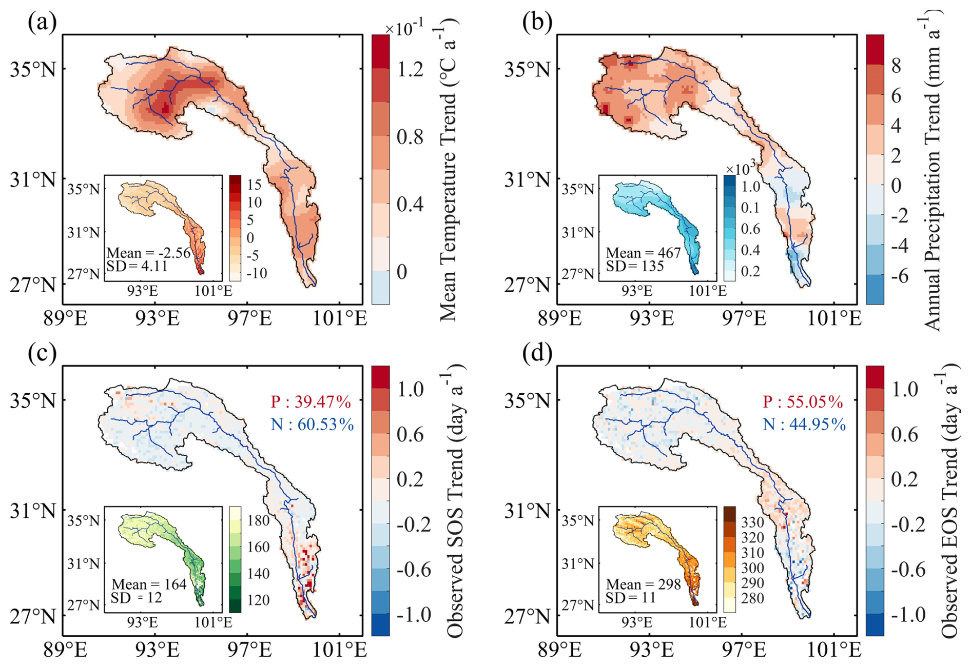
Figure 2 Spatial and temporal variations in climatic variables and vegetation phenology during 1982–2018. The inner plot of each panel depicts the spatial pattern of the multiyear means of each variable, with units of degrees Celsius (°C; a), millimeters (mm; b), and day of year (DoY; c, d). P, the percentage of pixels showing a positive trend, indicates delayed SOS and EOS; N, the percentage of pixels showing a negative trend, indicates decreased advanced SOS and EOS.

3 Results

3.1 Spatiotemporal variations in climate and vegetation phenology

There is notable spatiotemporal heterogeneity in the multiyear mean annual temperature and accumulated precipitation across the upper reaches of the Jinsha River watershed (Fig. 2a and b). The mean annual temperature exhibits a gradual increase from the upstream to the downstream areas. The annual accumulated precipitation is higher in the downstream region than in the upstream. In addition, the mean annual temperature and accumulated precipitation showed clear temporal trends during 1982–2018. The mean annual temperature significantly increased by 0.06°C yr⁻¹ on average. The annual accumulated precipitation across the entire watershed increased by 2.64 mm yr⁻¹. However, downstream regions exhibited a declining trend (Fig. 2b). Over the past 4 decades, the upper reaches of the Jinsha River watershed showed a “warming–wetting” trend in the upstream area and a “warming–drying” trend in some downstream areas.

During 1982–2018, the multiyear mean SOS and EOS in the upper reaches of the Jinsha River watershed were 164 ± 12 and 298 ± 11 (day of year, DoY), respectively (Fig. 2c and d). The mean SOS was initiated in early May downstream and early July upstream. The mean EOS occurred in early October upstream, 1 month earlier than downstream. The SOS advanced in 60.5 % of the study area over the past 4 decades, primarily in the middle and upper reaches of the watershed (−0.05 ± 0.13 d yr⁻¹) while being delayed by 0.09 ± 0.30 d yr⁻¹ in the downstream area. During the study period, the EOS was delayed by 0.08 ± 0.27 d yr⁻¹ in the downstream area but advanced by −0.03 ± 0.14 d yr⁻¹ in the upstream area. This spatiotemporal heterogeneity of vegetation phenology further highlights the importance of incorporating vegetation dynamics into hydrological models.

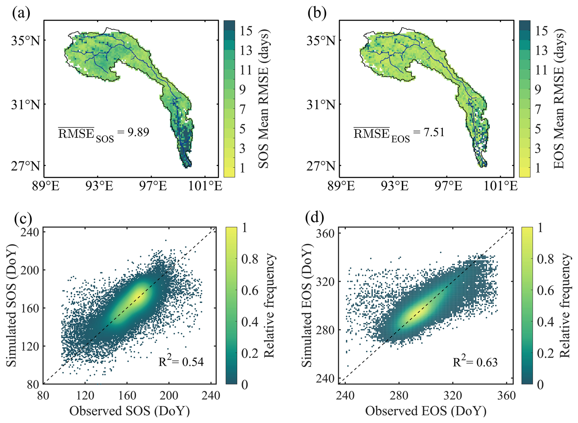
Figure 3 Performance of phenology module. Spatial patterns of the RMSE for start of season (SOS, a) and end of season (EOS, b). Scatter plots depicting the relationship between simulated and observed start of season (SOS, c) and end of season (EOS, d). The overlined RMSE represents the average RMSE. The colored points on the scatter plots represent kernel density, with lighter colors indicating a higher density distribution. The dashed line represents the 1:1 ratio line.

3.2 Performance of phenology module and modified SWAT-Carbon model

The mean RMSEs for the spring and autumn phenology models are 9.89 and 7.51 d, with calibration and validation RMSEs of 8.71 and 10.82 d for SOS and 7.03 and 7.77 d for EOS, respectively (Fig. 3a and b). Within the study area, 67.1 % and 85.8 % of pixels exhibited an RMSE of less than 10 d for SOS and EOS, respectively. The correlation coefficients between observed and simulated SOS and EOS were 0.54 and 0.63, respectively.

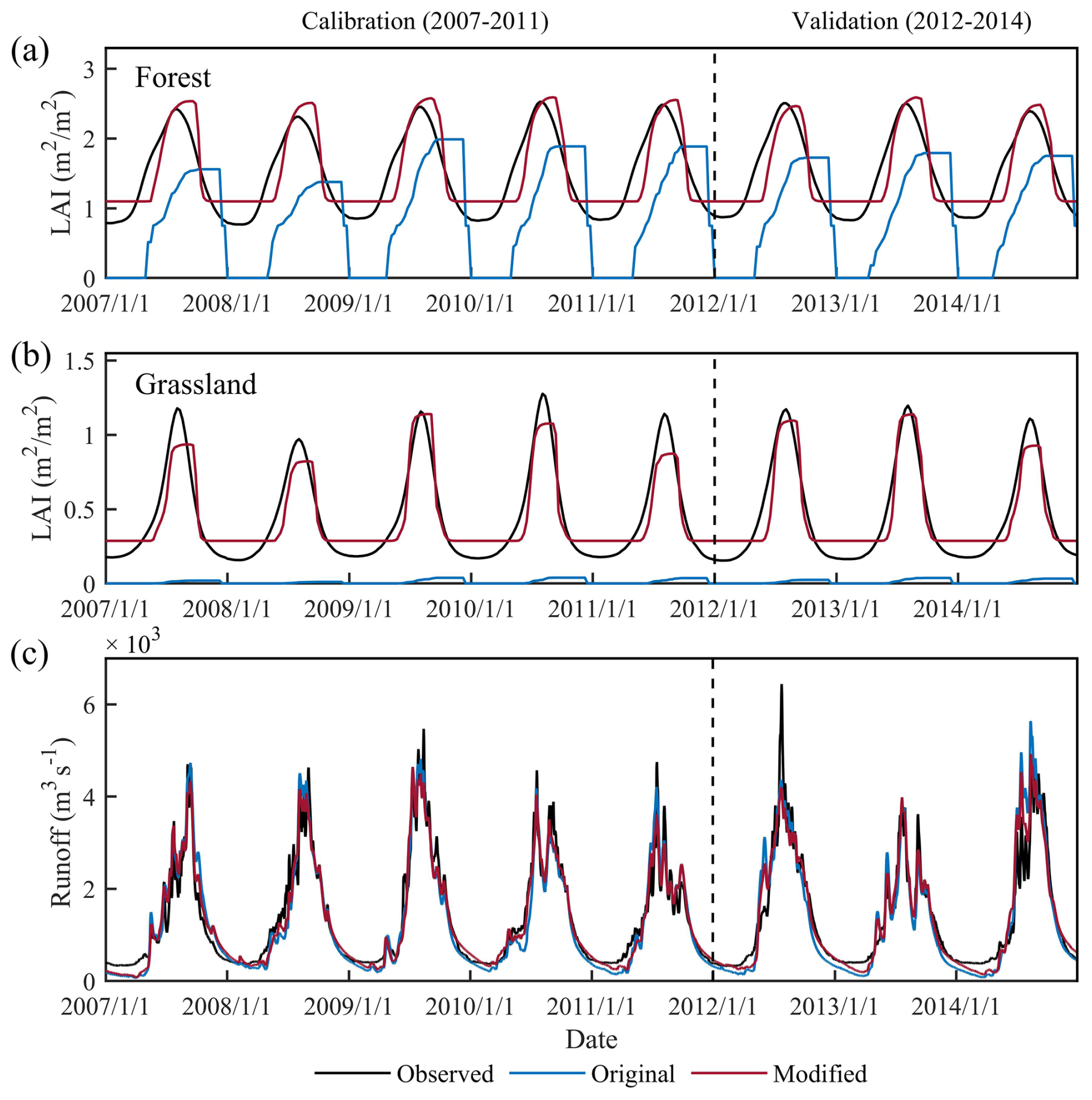
Figure 4 Temporal variability in the LAI and runoff during the calibration (2007–2011) and validation (2012–2014) periods. The 8 d LAI time series derived from satellite observations and simulated by the original and modified SWAT-Carbon models for forest (a) and grassland (b). Daily observed and simulated runoff by the original and modified SWAT-Carbon models (c).

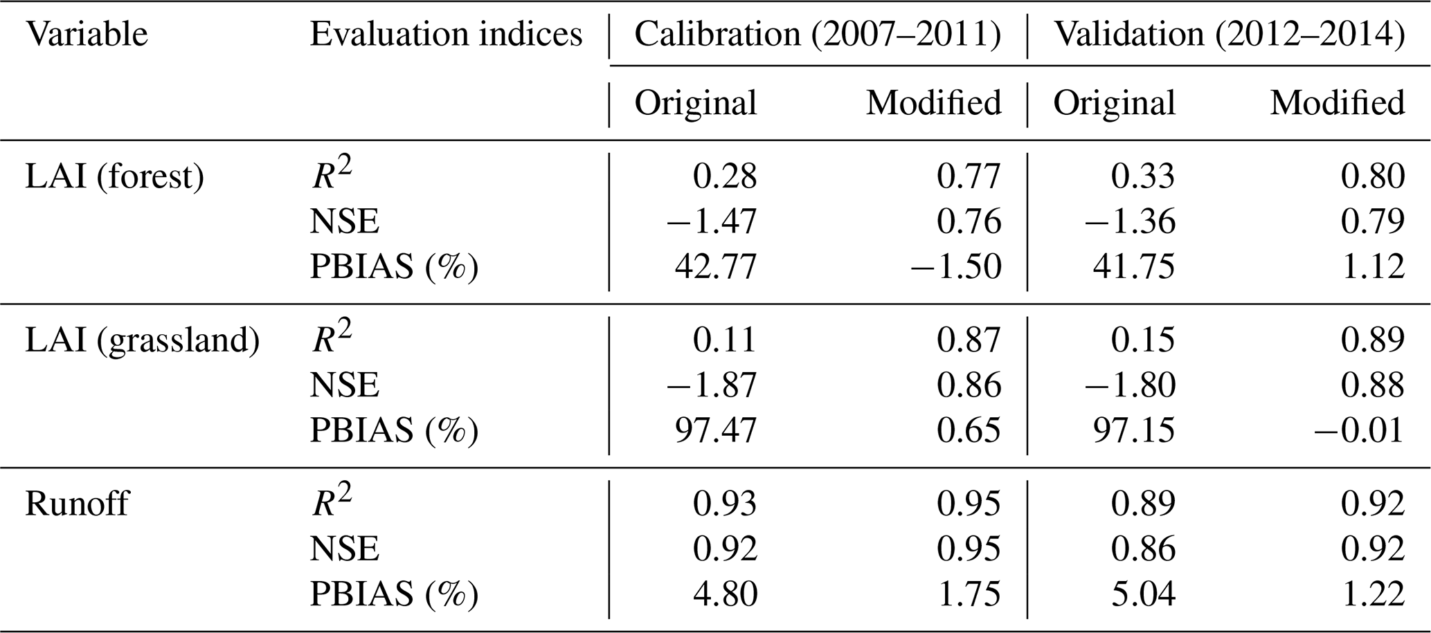
Table 2 Evaluation indices of the original and modified SWAT-Carbon model in simulating LAI and runoff. R² is the coefficient of determination, NSE the Nash–Sutcliffe efficiency, and PBIAS the percent bias.

In the modified SWAT-Carbon model, the fixed phenology dates were replaced by the outcomes of the phenology module, and the simulated LAI before the start of the growing season was changed to a non-zero value for both forest and grassland. After these modifications, the calibrated and validated LAI growth curves largely improved compared to the original model (Fig. 4a and b, Table 2). Specifically, the average R² and NSE values improved from 0.31 and −1.42 to 0.79 and 0.78 for forest and from 0.13 and −1.84 to 0.88 and 0.87 for grassland, respectively. Additionally, the absolute PBIAS decreased by 41.0 % for forest and 97.0 % for grassland. To further exclude the impact of non-growing-season LAI, we also adjusted the non-growing-season LAI to non-zero values in the original SWAT-Carbon model. The results indicated that, compared to the default settings, there were only slight improvements in the LAI growth curves in the original model (Fig. S1 in the Supplement). Specifically, the average NSE value improved from −1.42 to −0.29 for forest and from −1.84 to −0.70 for grassland, which is much smaller than the NSE for LAI in the modified model. Furthermore, the average R² decreased by 0.17 for forest and by 0.01 for grassland.

Incorporating the phenology module into the SWAT-Carbon model enhanced the performance of runoff simulation. The modified SWAT-Carbon model produced a runoff simulation with a “very good” level of performance (0.80 < R² ≤ 1 and 0.75 < NSE ≤ 1; Fig. 4c and Table 2). Furthermore, the performance of runoff simulation showed improvement in various months, particularly during the vegetation greening period (June), the senescence period (October), and the non-growing season (Table S3 in the Supplement). Specifically, the R² and NSE values for runoff increased by 0.13 and 0.39 in June, respectively, and by 0.30 and 0.46 in October. The NSE value for runoff from November of the previous year to May increased by 0.35.

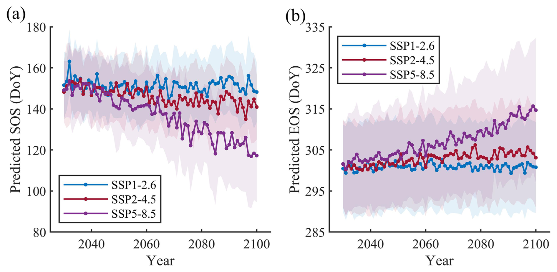
Figure 5 Projection of future spring and autumn phenology during 2030–2100. Future shifts at start of season (SOS, a) and end of season (EOS, b) under three Shared Socioeconomic Pathway (SSP) scenarios based on the Coupled Model Intercomparison Project Phase 6 (CMIP6) multimodel ensemble. SSP1-2.6, SSP2-4.5, and SSP5-8.5 refer to low, moderate, and high emissions, respectively. Colored lines and shading represent the mean and 1 standard deviation across the four CMIP6 models under each emission scenario.

3.3 Future shifts in vegetation phenology and runoff

The UniChill and DM phenology models were used to project future shifts in SOS and EOS during 2030–2100 under different emission scenarios. The SOS in the upper reaches of the Jinsha River watershed was projected to advance under all scenarios (Fig. 5a), with the most significant advancement observed under the high-emission scenario (0.49 d yr⁻¹, p < 0.01). In addition, a delay in EOS was observed under all scenarios (Fig. 5b), with the largest delay occurring under the high-emission scenario (0.18 d yr⁻¹, p < 0.01).

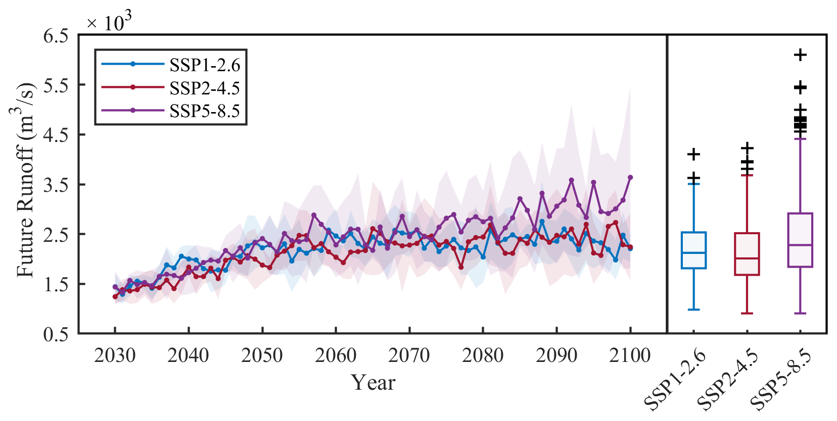
Figure 6 Projection of future runoff during 2030–2100 using the modified SWAT-Carbon model. Colored lines and shading in the right subplot represent the mean and 1 standard deviation across the four CMIP6 models. The scenarios SSP1-2.6, SSP2-4.5, and SSP5-8.5 refer to low emissions, moderate emissions, and high emissions, respectively. The cross symbol represents the outlier.

The runoff under the SSP5-8.5 scenario exhibited greater fluctuation with a continuous increase from 2030 to 2100. Specifically, runoff was projected to increase from approximately 1437 m³ s⁻¹ in 2030 to 3638 m³ s⁻¹ in 2100. However, the runoff under the SSP1-2.6 and SSP2-4.5 scenarios was projected to initially increase and then stabilize after 2060 (Fig. 6). The average runoff under SSP5-8.5 (2459 m³ s⁻¹) was greater than that under SSP1-2.6 (2180 m³ s⁻¹) and SSP2-4.5 (2120 m³ s⁻¹). Results from the original SWAT-Carbon model showed a smaller increase in future runoff compared to that estimated by the modified SWAT-Carbon model (Fig. S2 in the Supplement). Monthly total runoff outputs were obtained from CMIP6 models and aggregated to annual runoff from 2030 to 2100. We calculated the watershed-scale future runoff from CMIP6 using the area-weighted mean method and found that the future runoff from CMIP6 models was larger than that simulated by the modified SWAT-Carbon model (Fig. S3 in the Supplement).

4 Discussion

4.1 Improvement of runoff simulation by modified hydrological model

Vegetation phenology exerts strong controls over seasonal and annual hydrological processes (Kim et al., 2018; Yang et al., 2023). However, the vegetation phenology in most hydrological models, such as the SWAT-Carbon model, is based on simple thermal and day-length thresholds (Arnold et al., 1998). This approach results in large uncertainty in simulating vegetation dynamics and thereby in projecting hydrological processes, especially under climate change (Zhang et al., 2009; Ma et al., 2019; Wang et al., 2022). In this study, we integrated process-based spring and autumn phenology models into the SWAT-Carbon model, which substantially improved the simulation of vegetation dynamics and ecohydrological processes. The simulation of the LAI curve, particularly in terms of seasonality and magnitude, exhibited significant improvement in the modified SWAT-Carbon model (Fig. 4a and b, Table 2). The inaccuracy of LAI simulation in the original model was attributed to the initiation and end of vegetation dormancy being determined only by a latitude-based day-length threshold. This approach leads to mismatches in the timing of phenological stages in the LAI curve compared to observed data (Figs. 4a and b and S1). Based on the widely used process-based phenological models (Fu et al., 2020), we incorporated the phenology module into the SWAT-Carbon model, which provides a method for accurately simulating the timing of vegetation growth stages and the runoff. In addition, the highest and lowest simulated LAI values in the original model showed significant underestimation. This is attributed to the inability to meet the default constant value of heat accumulation requirements, owing to low daily temperatures in the upper reach of the Jinsha River watershed. In the modified model, we replaced the constant value with a dynamic heat accumulation requirement and optimized vegetation growth parameters, which finally enhanced the simulation accuracy of LAI values and thereby improved runoff simulation. Therefore, we highlight the importance of integrating the phenology module into hydrological models.

Our study indicated that the modified SWAT-Carbon model improved the simulation of vegetation and runoff. However, some uncertainties from the dataset and model persist in the modified model and should be addressed. The meteorological input data used in this study were obtained from gridded datasets which may differ from actual conditions. In addition, climate-sensitive ecosystem structures, such as species composition, introduce uncertainties in assessing interactions between vegetation phenology and hydrological processes in the modified SWAT-Carbon model (Chuine, 2010; Huang et al., 2019). Therefore, coupling advanced land surface models, such as LPJ-GUESS (Sitch et al., 2003), with hydrological models could further improve our understanding of future vegetation dynamics and their effects on the carbon and water cycles.

4.2 Interaction between vegetation phenology and hydrological processes

Our results indicated significant improvement in the performance of runoff simulation, particularly during the vegetation greening period (June) and the senescence period (October) (Tables 2 and S3), which is attributed to the accurate phenology prediction. Vegetation phenology and hydrological processes are closely intertwined through biotic and abiotic pathways (Buermann et al., 2018; Lian et al., 2020). In the upper reaches of the Jinsha River watershed, the multiyear mean SOS and EOS occurred in June and October (Fig. 2), respectively. During the start and end of the growing season, rapid changes in vegetation physiological properties, such as stomatal conductance and LAI, influence the timing and amount of water resource allocation (Zhang et al., 2021; Hwang et al., 2023).

In addition, the vegetation dynamics and their impacts on the underlying land surface properties affect watershed evapotranspiration (Chen et al., 2022b). To explore the response of ET to vegetation phenology in the upper reaches of the Jinsha River watershed, we analyzed the relationship between the phenological variations and subbasin-scale ET using the modified SWAT-Carbon model. Consistent with previous studies in the Northern Hemisphere, our study revealed a positive correlation between ET and growing season length (Fig. 7), potentially attributed to the prolonged period of water movement from the soil to the atmosphere (Geng et al., 2020; Yang et al., 2023). This was further verified by the observation that earlier leaf unfolding and delayed leaf senescence increased spring and autumn ET. Vegetation phenology influences the development and decay of the canopy, altering the water demands of vegetation and affecting the hydrological cycle (Hwang et al., 2018; Lian et al., 2020). However, our study found that both spring and autumn ET increased by similar magnitudes, with values of 1.58 and 1.62 mm d⁻¹, respectively. This finding is inconsistent with the asymmetrical increase reported in previous research (Kim et al., 2018), which may be attributable to the abundant soil moisture during summer in our study area. This moisture abundance does not impose constraints on vegetation growth and transpiration.

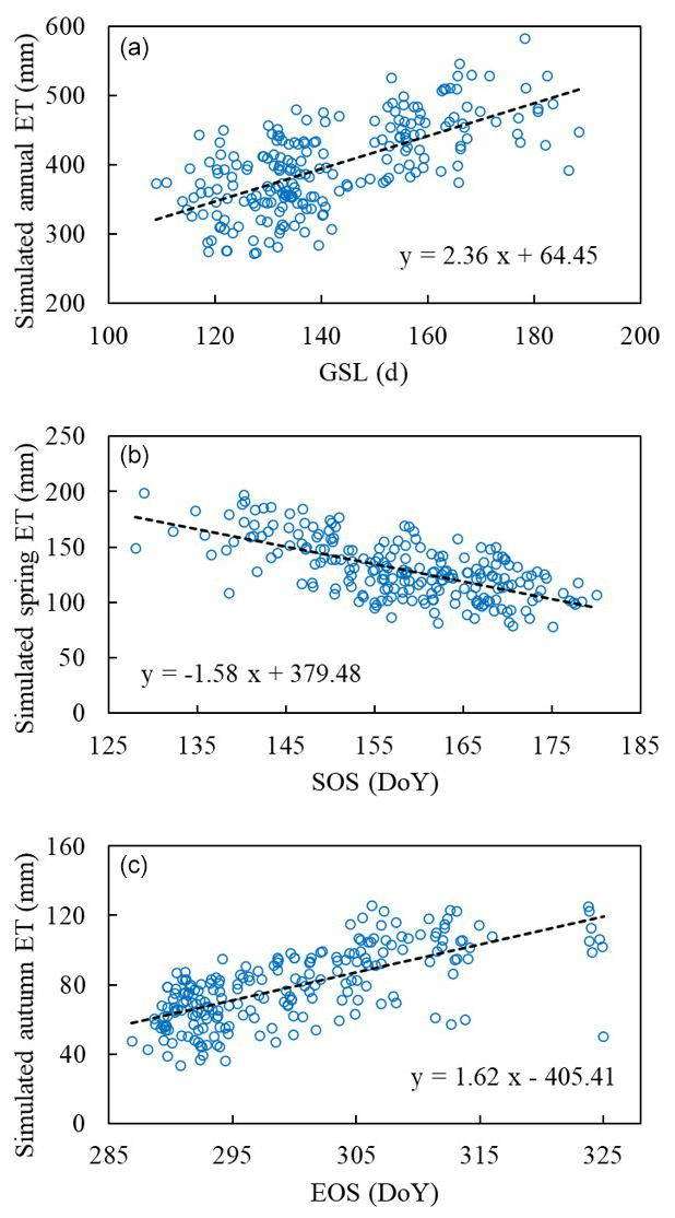
Figure 7 Relationship between the phenological variations and subbasin-scale evapotranspiration (ET) using modified SWAT-Carbon model. Relationship between growing season length (GSL) and annual ET (a), relationship between start of season (SOS) and spring ET (b), and relationship between end of season (EOS) and autumn ET (c).

4.3 Hydrological response to future climate change and vegetation dynamics

We projected future runoff in the upper reaches of the Jinsha River watershed and found that the runoff would largely increase under future climate change conditions. Specifically, under the SSP5-8.5 scenario, runoff exhibited the most pronounced upward trend, primarily attributed to increased precipitation largely surpassing that of the SSP1-2.6 and SSP2-4.5 scenarios (Figs. 6 and S4 in the Supplement). In addition to precipitation, the advanced SOS and delayed EOS under global warming (Fig. 5), which were projected in the upper reaches of the Jinsha River watershed, also play an important role in altering the water cycle. Despite a substantial increase in precipitation under SSP2-4.5 compared to SSP1-2.6, the projected runoff under SSP2-4.5 is marginally smaller than that under SSP1-2.6. This phenomenon is likely attributed to the extension of the growing season under global warming, which significantly increases evapotranspiration under the moderate emission pathway compared to the low-emission pathway (Lu et al., 2021; Yang et al., 2023). The increased precipitation under SSP2-4.5 is insufficient to fully counteract the increase in evapotranspiration caused by the prolonged growing season (Fig. S4 in the Supplement).

In this study, future runoff simulation by the original SWAT-Carbon model is smaller than that by the modified model, especially under the high-emission scenario, which is also observed in the historical runoff (Fig. 4c). The underestimation of the historical runoff simulation is attributed to lower baseflow compared to observed data, particularly during the non-rainy season. This discrepancy is potentially influenced by underestimated LAI simulations and unreasonable parameters in the original SWAT-Carbon model (Tang et al., 2022). Vegetation degradation was reported to reduce flow during the dry season (Paiva et al., 2023). In addition, although calibration algorithms enhance the original model's ability to produce accurate runoff simulations, the unrealistic representation of vegetation phenological processes necessitates remediation through additional ecohydrological processes (Haas et al., 2022; Luan et al., 2022), thereby compromising the model's fidelity. Therefore, improving the simulation accuracy of vegetation dynamics could enhance the capability of hydrological models to accurately depict ecohydrological processes, especially in the dry season, thereby facilitating more effective water resource conservation strategies under future global warming.

5 Conclusions

In summary, our study integrated a process-based vegetation phenology module into the SWAT-Carbon model, substantially improving the simulation of vegetation dynamics and hydrological processes in the upper reaches of the Jinsha River watershed. The runoff is predicted to increase over 2030–2100 under different future emission scenarios, primarily due to greater precipitation outweighing the increase in evapotranspiration induced by the prolonged growing season. Our study highlights the importance of integrating phenological shifts into hydrological models. In the future, it will be crucial to consider and couple plant functional types with hydrological models to further enhance the performance of ecohydrological process simulations. Furthermore, the phenology module should be incorporated into other hydrological models and applied in various watersheds to enhance our understanding of ecohydrological processes and to support future water resource management under climate change conditions.