Technical note: Quadratic Solution of the Approximate Reservoir Equation (QuaSoARe)

This paper presents a method to solve the reservoir equation, a special type of scalar ordinary differential equation controlling the dynamic of conceptual reservoirs found in most hydrological models. The method, called the “Quadratic Solution of the Approximate Reservoir Equation” (QuaSoARe), applies to any reservoir equation regardless of its non-linearity or the number of fluxes entering and leaving the reservoir. The method is based on a piecewise quadratic interpolation of the flux functions, which leads to an analytical and mass-conservative solution. It is applied to two routing models and two rainfall–runoff stores that are representative of hydrological model components, and it is evaluated based on six catchments in eastern Australia that experienced one of the most extreme floods in recent Australian history. A comparison of the method against two standard numerical schemes, the fifth-order Radau implicit Runge–Kutta scheme and the explicit Runge–Kutta scheme of order 5(4), suggests that it can reach similar accuracy while reducing runtime by a factor of 10 to 50 depending on the model considered. At the same time, the method is simple enough to be presented as a short pseudo-code, which is included in this paper. Beyond solving a given reservoir equation, the method constitutes a promising avenue to define flexible models where flux functions are defined as piecewise quadratic functions, which can be solved exactly with QuaSoARe.

1 Introduction

1.1 Reservoirs as ubiquitous components of environmental models

Environmental models, including hydrological models, often rely on components that can be modelled conceptually as a reservoir receiving inputs and generating outputs that are sole functions of the volume stored in the reservoir. Such reservoirs are extensively used in rainfall–runoff models such as GR4J (Perrin et al., 2003), HBV (Bergstrom and Forsman, 1973), IHACRES (Croke and Jakeman, 2004), and SAC-SMA (Burnash and Ferral, 1981), where the reservoir dynamic is described by a differential equation relating the change in storage to input and output fluxes. If the model is applied to a time step long enough for storage to change significantly, this equation must be integrated to obtain the storage level at the end of the time step and the total of each flux. However, apart from a few simple cases, there is no analytical solution to this mathematical problem, and one has to revert to numerical approximations (Clark and Kavetski, 2010; Kavetski and Clark, 2010). Furthermore, flux functions in hydrological models are often highly non-linear, which magnifies numerical errors when using inappropriate numerical schemes (Kavetski and Clark, 2011). This, in turn, degrades model simulation and calibration due to the extra parameterisation needed to compensate for these errors (Kavetski et al., 2006). In this context, this paper presents an approximate analytical method called the “Quadratic Solution of the Approximate Reservoir Equation” (QuaSoARe) to solve the scalar ordinary differential equation (ODE) underlying most conceptual reservoirs used in hydrology.

The integration of ODEs represents an entire field in applied mathematics, with a history as old as differential calculus. The reader might wonder why a paper is needed for such a well-beaten scientific track. Despite the voluminous literature written on the topic, the large number of software packages available, and the importance of proper ODE integration flagged by Kavetski and Clark (2010), the use of proven ODE numerical schemes remains rare in hydrological modelling. We suggest that this troubling fact may come about because the methods described in reference textbooks (Hairer et al., 2009; Shampine, 2020) aim to solve very general ODEs and hence require complex algorithms to handle every extreme scenario in the equation set-up. However, this complexity might be superfluous if one wants to solve a simple scalar equation such as a conceptual reservoir used in hydrological modelling. This paper aims to bridge this gap by proposing a simple yet effective and mass-conservative approximate solution designed specifically for the scalar reservoir equation ODE.

More precisely, let us denote the volume stored in the reservoir by S and assume that the reservoir is submitted to forcing variables $\stackrel{\mathrm{̃}}{V}$ that remain constant over the time step. This assumption corresponds to most practical hydrological modelling scenarios where the time distribution of the forcings during the time step is unknown (e.g. time average of rainfall or potential evapotranspiration). In this case, the reservoir equation ODE is formulated as follows:

$$\begin{array}{}\text{(1)}& {\displaystyle \frac{\mathrm{d}S}{\mathrm{d}t}}={\sum }_{i=\mathrm{1}}^n{f}_i\left(S,\stackrel{\mathrm{̃}}{V}\right),\end{array}$$

where f_i denotes arbitrary continuous functions representing input or output fluxes from the reservoir. Here, it is assumed that the f_i functions are Lipschitz continuous, which ensures that Eq. (1) has a unique solution (Hairer et al., 2009). We also assume that Eq. (1) is input-to-state stable, which guarantees that its solution is bounded if the inputs $\stackrel{\mathrm{̃}}{V}$ are bounded (Mironchenko, 2023). Note that demonstrating the global stability of an ODE is a complex problem much beyond the scope of this paper. LaSalle (1960) presented a method using Lyapunov functions, which were later generalised by Sontag (1989) for systems such as Eq. (1). The mathematical assumptions made here and the theoretical limitations they introduce are further discussed in Sect. 4.

Solving Eq. (1) is an initial value problem over a time interval [0, δ], where δ is the time step. S₀ is defined as the initial condition at t=0. To obtain a simulation from the reservoir, Eq. (1) is solved repeatedly for each time step with varying forcing variables (e.g. a daily series of rainfall values). It is highlighted that the presence of several functions f_i in Eq. (1) is common in hydrological models, for example, to account for multiple runoff generation processes such as infiltration and overland flow or fluxes between surface water and groundwater stores (Clark et al., 2008). Other model components often require these fluxes (e.g. infiltration excess runoff being used as input into a routing model), which means that, in addition to solving for variable S, one must compute the total of each flux over the time step given by

$$\begin{array}{}\text{(2)}& O_i=\underset{\mathrm{0}}{\overset{\mathit{\delta }}{\int }}{f}_i\left(S,\stackrel{\mathrm{̃}}{V}\right)\mathrm{d}t.\end{array}$$

It is important to note that the computation of O_i does not affect the solution S(t). To follow the terminology of atmospheric modelling, O_i is a diagnostic variable (American Meteorological Society, 2024), whereas S is a prognostic variable.

Equation (1) has a broad range of applications beyond hydrological modelling, for example, to estimate storage in an artificial reservoir (Fiorentini and Orlandini, 2013) or to solve the gradually varied flow equation in hydraulics (Gill, 1976). Unfortunately, there are very few cases where both Eqs. (1) and (2) have an analytical solution, a problem that is considerably more difficult than solving Eq. (1) alone. Consequently, most reservoir equations are solved using numerical approximation methods.

1.2 Numerical methods to solve the reservoir equation

The most common approach relies on discrete methods that estimate S from t=0 to δ at incremental steps using Runge–Kutta methods (Kavetski and Clark, 2010; Knoben et al., 2019; La Follette et al., 2021). These schemes are the topic of a voluminous literature, including several reference textbooks (Butcher, 2003; Hairer et al., 2009; Press et al., 2007; Shampine, 2020, to name but a few). Nonetheless, applying them requires significant expertise to (1) select the most appropriate scheme among the multiple variants available (e.g. Euler, Runge–Kutta, or Huen schemes), (2) decide if the scheme is explicit (where the solution depends on S₀ only) or implicit (where it depends on both S₀ and S(δ), which requires iterative optimisation), and (3) choose between fixed or variable step lengths to automatically slow down computation when facing numerical difficulties. These choices are not trivial and far from harmless, as warned by Michel et al. (2003) and Kavetski and Clark (2011), who show the disastrous consequences of solving the exponential store with an explicit Euler scheme. As a result, these techniques are not simple to code, and a modeller unfamiliar with them will often require a third-party software package. This adds a dependency to the model code, complicates maintenance, and increases runtime, sometimes significantly when using implicit methods compared to an analytical solution. At the same time, despite the exponential growth of computing power, runtime is still a limiting factor in hydrology when a large number of runs is required, for example, in a Monte Carlo uncertainty analysis or for the calibration of distributed models.

In addition, besides applying the right ODE integrator to Eq. (1), solving the reservoir equation requires a numerical integration of Eq. (2) using a potentially different algorithm. For example, a simple quadrature method can be used to estimate the integral on the right-hand side of Eq. (2) based on the two values S₀ and S(δ). However, this approach can be highly inaccurate if the solution s(t) does not vary linearly with time, as demonstrated in the Supplement. A more accurate method is to expand Eq. (1) into a system of differential equations by adding one differential equation for each flux:

$$\begin{array}{}\text{(3)}& {\displaystyle \frac{\mathrm{d}{O}_i}{\mathrm{d}t}}=f_i\left(S,\stackrel{\mathrm{̃}}{V}\right)i=\mathrm{1},\mathrm{\dots }n.\end{array}$$

The solution can then be obtained by applying the selected integrator to the system of ODEs combining Eqs. (1) and (3). However, because of the wide range of magnitudes observed in hydrological fluxes, this may lead to a system that could be characterised as “stiff” and for which many numerical schemes become unstable (Kavetski and Clark, 2011; Shampine, 2020).

Another angle of attack for solving an ODE is to replace the original equation with one for which an analytical solution exists. With the simplest ODEs being linear, it is not surprising that linearisation of Eq. (1) around a specific regime (e.g. steady-state) has constituted the first approach proposed by mathematicians (Hartman, 2002). Linearisation has often been used to solve complex differential equations in hydrology and hydraulics, for example, the Saint-Venant 1D hydrodynamic equation by Hayami (1951) or, more recently, those by Fan and Li (2006) or Munier et al. (2008). This approach is efficient if the true solution does not depart significantly from the linearisation regime. Unfortunately, hydrological systems often exhibit variations of several orders of magnitude that violate this assumption. A logical extension of the linearisation approach is to define several linear approximation regimes between which the solution can switch. This idea has been explored extensively in the control literature (Johansson, 2003), starting with the early work by Kalman (1955). More recently, this approach has been formalised in the field of electrical engineering under the name trajectory piecewise-linear approximation (TPLA), a method introduced by Rewienski and White (2003) to solve large non-linear differential equation systems. The theory presented by Rewienski and White (2003), along with its subsequent refinements (Bond and Daniel, 2009; Kalra and Nabi, 2020), aims to solve equation systems far more complex than the reservoir equation studied here. Adapting this theory for the scalar reservoir equation, along with a clear algorithmic description, would be a valuable contribution from this study. In addition, the TPLA theory relies on a transition between linearised states which is not necessarily continuous. Finally, the choice of the transition function is arbitrary, which adds subjectivity to the process and does not guarantee that the derivative of the solution remains continuous. This can be an issue if the model shows strong non-linearity. This problem was raised by Litrico et al. (2010), who proposed a continuous linearisation method to approximate the Saint-Venant hydrodynamic equations. Overall, the TPLA method is useful for representing complex non-linear dynamics. Still, a simpler approach restricted to a scalar system such as the reservoir equation would likely make its adoption easier. Extending the linearisation idea, Pope (1963) introduced the concept of an exponential integrator, where the linearisation of an ODE is combined with a discrete method such as a Runge–Kutta scheme applied to the residual between the linearised part and the original function. Hochbruck and Ostermann (2006) demonstrated this method's efficacy in solving large systems of stiff equations. However, its reliance on a discrete method to correct the linearised solution faces the same issues raised earlier for an application to hydrological models.

Overall, the review of the literature above highlighted the following research gaps:

• The reservoir equation is a standard tool in hydrology that requires fast and robust numerical solutions in the absence of general analytical approaches.

• Classical ODE numerical solvers such as Runge–Kutta methods are not straightforward, especially if the equations are stiff and lead to potentially unstable solutions.

• Existing theoretical developments from control theory based on multiple linearisation points are complex and require care when switching between linearised regimes.

1.3 Objectives of the paper

This paper aims to

• present an approximate analytical solution for the reservoir equation, with the solution solving Eq. (1) and computing all input and output fluxes from Eq. (2);

• demonstrate the application of the method to four reservoir equations of increasing complexity and non-linearity and to compare the results with classical implicit and explicit discrete methods.

The method, including its pseudo-code, is presented in Sect. 2.2 and 2.3, while an accompanying Python package is released as supporting material. Section 4 details some limitations of the method and recommendations to remediate them. The protocol used to compare the method with existing discrete methods is detailed in Sect. 5, with results being presented in Sect. 6 and discussed in Sect. 7. The paper is concluded in Sect. 8.

2 Approximate analytical solution of the reservoir equation using piecewise quadratic functions

The method presented in this section is inspired by the TPLA and exponential-integrator methods, where the functions f_i in Eq. (1) are approximated by functions for which an analytical solution of the reservoir equation exists.

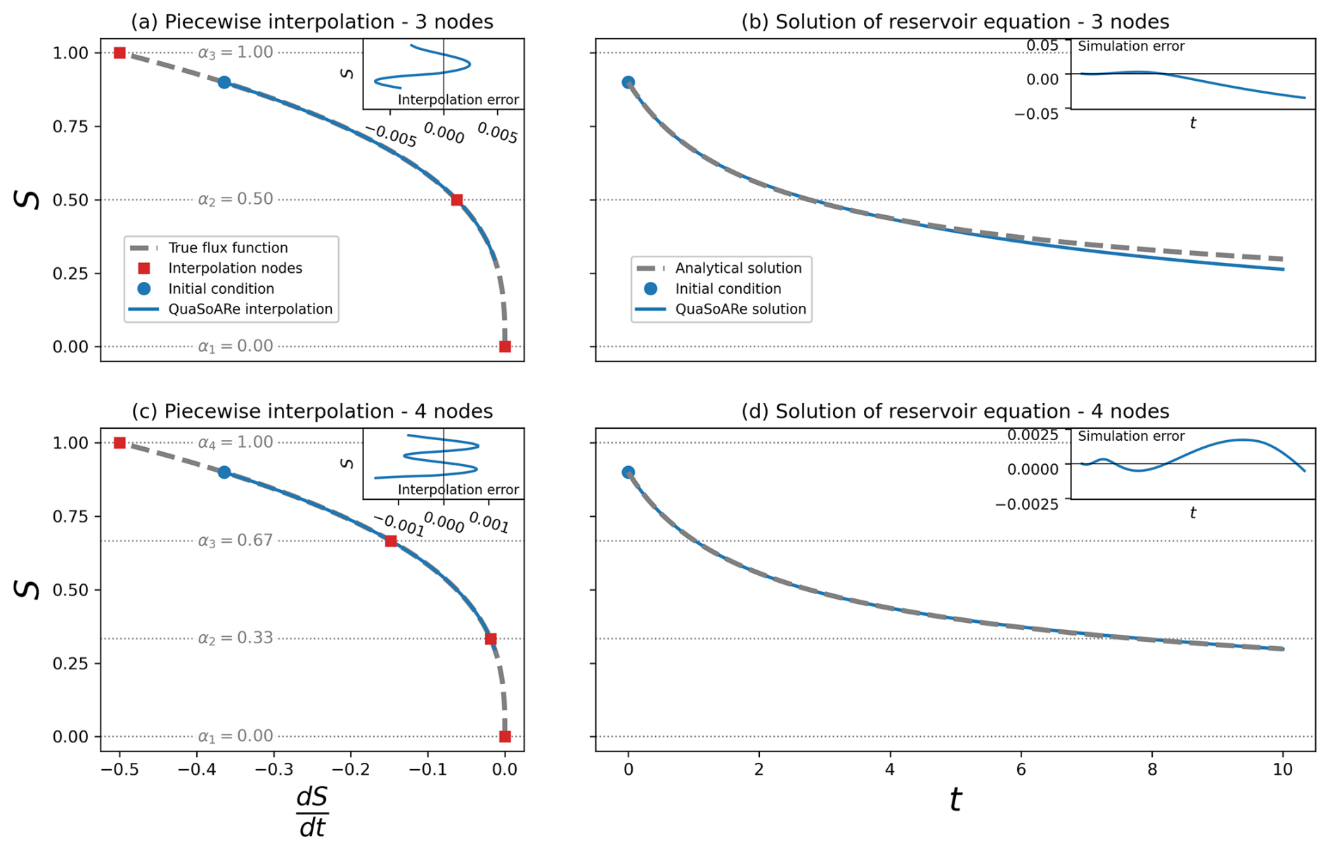
Figure 1 QuaSoARe method applied to the example reservoir equation. The left plots (a, c) present the reservoir equation (i.e. the right-hand side of Eq. 4) as a dashed grey line and its QuaSoARe approximation as a blue line. The right plots (b, d) show this equation's analytical and QuaSoARe solutions using the same colours. A QuaSoARe configuration with three interpolation nodes is used in the two top plots (a, b), while four nodes are used in the two bottom plots (c, d).

2.1 Illustrative example

Before presenting the method, an illustrative example using the following reservoir equation is introduced:

$$\begin{array}{}\text{(4)}& {\displaystyle \frac{\mathrm{d}S}{\mathrm{d}t}}=-{\displaystyle \frac{S^{\mathrm{3}}}{\mathrm{2}}}.\end{array}$$

This equation is a special case of the cubic flow-routing model, further discussed in Sect. 5.1. Assuming an initial condition S₀ at t=0, the analytical solution of Eq. (4) is as follows:

$$\begin{array}{}\text{(5)}& s\left(t\right)={\displaystyle \frac{S_{\mathrm{0}}}{\sqrt{\mathrm{1}+t{S}_{\mathrm{0}}^{\mathrm{2}}}}}.\end{array}$$

The reservoir equation function from the right-hand side of Eq. (4) is plotted in Fig. 1a as a dashed grey line. The corresponding solution from Eq. (5) is shown in Fig. 1b as a dashed grey line using a value of S₀ equal to 0.9. Other elements in this figure are related to the QuaSoARe method and are described in the following sections.

2.2 Reservoir equation approximation by quadratic functions

Before presenting the approximate solution, it needs to be established that the solution s(t) of Eq. (1) is monotonic, a result that is used repeatedly across this paper. This can be proved by contradiction: let us assume that s(t) is not monotonic. Consequently, s being derivable as a solution of Eq. (1), there exists a time t₀>0 where the derivative of s changes sign, and $\mathrm{d}s/\mathrm{d}t\ne \mathrm{0}$ for t>t₀. Let us now introduce the function s₂, which is identical to s for t<t₀ and which remains constant and equal to s(t₀) for t≥t₀. This function is a solution of Eq. (1) for all t>0 and is distinct from s for t>t₀ because its derivative is zero, while the derivative of s is not. This is a contradiction, with the uniqueness of the solution of Eq. (1) being imposed by the fact that f is Lipschitz continuous, as stated in the previous section. Consequently, s is monotonic for t≥0.

Back to solving Eq. (1), let us assume that each function f_i can be approximated by a function $f_i^{\ast }$ written as follows:

$$\begin{array}{}\text{(6)}& f_i^{\ast }(S,\stackrel{\mathrm{̃}}{V})={\sum }_{j=\mathrm{1}}^{m-\mathrm{1}}\left[a_{i,j}{S}^{\mathrm{2}}+b_{i,j}S+c_{i,j}\right]I_j\left(S\right),\end{array}$$

where the series ${\mathit{\alpha }}_{\mathrm{1}}<{\mathit{\alpha }}_{\mathrm{2}}<\mathrm{\dots }<{\mathit{\alpha }}_m$ defines a partitioning of the interval [α₁,α_m] into m−1 intervals referred to as “interpolation bands”. In addition, the interval [α₁, α_m] is assumed to contain the bounds of s(t) (the solution to Eq. 1 is assumed to be bounded in Sect. 1.1). I_j(x) is the indicator function equal to 1 if $x\in [{\mathit{\alpha }}_j,{\mathit{\alpha }}_{j+\mathrm{1}}[$ and equal to zero elsewhere. The α_j values are referred to as “interpolation nodes” in this paper. The coefficients a_i,j, b_i,j, and c_i,j are independent of S. The process to obtain a_i,j, b_i,j, and c_i,j is detailed in Appendix A so that the approximated function $f_i^{\ast }$ matches the original function f_i at the nodes α_j and at the midpoint between α_j.

The approximation described above is applied to the example equation given in Eq. (4): two approximations are presented in Fig. 1a and c using three and four nodes, respectively. Both lead to a highly accurate interpolation where true and approximated functions are visually indistinguishable. The interpolation error, that is, the difference between the true function and its approximated counterpart, is shown as an inset in both plots. This error is reduced by a factor of approximately 5 when the number of nodes increases from three to four.

The form of Eq. (6) was chosen for several reasons. First, a piecewise quadratic function is Lipschitz continuous on a bounded interval. As a result, the solution to the corresponding reservoir equation, referred to as the approximated reservoir equation, is unique like the one of Eq. (1). Second, this equation can be solved analytically, as is shown in Sect. 2.3. Third, a quadratic function can approximate a wide range of reservoir functions used in hydrology. For example, if $a_{i,j}=\mathrm{0}$, the equation becomes a linear function of S, which is the most common reservoir equation used in hydrology. Finally, the steady-state solution of the approximate reservoir equation (i.e. when the derivative of S is zero) can be determined analytically, which greatly facilitates the analysis of the behaviour of the reservoir and the selection of α_j as discussed in Sect. 3. However, despite these appealing attributes, there are also downsides to this approximation, which are presented in Sect. 4, along with potential remediation.

Replacing the original functions f_i by their approximated counterpart $f_i^{\ast }$, the approximate reservoir equation is

$$\begin{array}{}\text{(7)}& \begin{array}{rl}{\displaystyle \frac{\mathrm{d}S}{\mathrm{d}t}}& ={\sum }_{i=\mathrm{1}}^n{f}_i^{\ast }(S,\stackrel{\mathrm{̃}}{V})\\ & ={\sum }_{j=\mathrm{1}}^m\left[A_j{S}^{\mathrm{2}}+B_{j}S+C_j\right]I_j\left(S\right),\end{array}\end{array}$$

where A_j, B_j, and C_j are the sums of the flux coefficients for the interpolation band j. For example, A_j is given by

$$\begin{array}{}\text{(8)}& A_j={\sum }_{i=\mathrm{1}}^n{a}_{i,j}.\end{array}$$

Importantly, Eq. (7) maintains an equality between the change in storage and the sum of the fluxes, meaning it conserves mass. This statement is trivial, but it ensures that the QuaSoARe algorithm generates mass-conservative simulations, which is a key requirement in hydrological modelling and is not always guaranteed by ODE numerical schemes, as pointed out by Clark and Kavetski (2010).

2.3 Analytical solution of the approximated reservoir equation

The solution to Eq. (7) can be obtained analytically as follows. Let us assume that the initial condition S₀ falls in the interpolation band $[{\mathit{\alpha }}_{j_{\mathrm{0}}},{\mathit{\alpha }}_{j_{\mathrm{0}}+\mathrm{1}}[$ where $j_{\mathrm{0}}\in [\mathrm{1},m-\mathrm{1}]$. For example, j₀=2 (second band) when S₀=0.9 in the illustrative example shown in Fig. 1a. When S₀ falls into the j₀th interpolation band at t=0, Eq. (7) can be simplified as follows:

$$\begin{array}{}\text{(9)}& {\displaystyle \frac{\mathrm{d}S}{\mathrm{d}t}}=A_{j_{\mathrm{0}}}{S}^{\mathrm{2}}+B_{j_{\mathrm{0}}}S+C_{j_{\mathrm{0}}}.\end{array}$$

The solution of this equation has an analytical expression, referred to as s(t). In addition, all fluxes from Eq. (2) can also be computed analytically. The process to obtain these expressions is not complex but tedious, and so its presentation is deferred to Appendix B. Using solution s(t), one can compute the value s(δ) at the end of the time step, leading to three cases:

• Case 1. s(δ) lies in the interval $[{\mathit{\alpha }}_{j_{\mathrm{0}}},{\mathit{\alpha }}_{j_{\mathrm{0}}+\mathrm{1}}[$. Because it is monotonic (see beginning of Sect. 2.2), s(t) remains bounded by ${\mathit{\alpha }}_{j_{\mathrm{0}}}$ and ${\mathit{\alpha }}_{j_{\mathrm{0}}+\mathrm{1}}$ for all t in [0,δ]. Consequently, Eq. (7) remains identical to Eq. (9) for $t\in [\mathrm{0},\mathit{\delta }]$, which means that s(t) is the solution of equation Eq. (7) over the interval [0, δ].

• Case 2. $s\left(\mathit{\delta }\right)<{\mathit{\alpha }}_{j_{\mathrm{0}}}$. Here, s(t) is a continuous function, with $s\left(\mathrm{0}\right)=S_{\mathrm{0}}\ge {\mathit{\alpha }}_{j_{\mathrm{0}}}$ and $s\left(\mathit{\delta }\right)<{\mathit{\alpha }}_{j_{\mathrm{0}}}$. Hence, by the intermediate-value theorem, there exists a time t_l<δ such that $s\left(t_l\right)={\mathit{\alpha }}_{j_{\mathrm{0}}}$. Moreover, s(t) is decreasing, which means that s(t) remains in the interval $[{\mathit{\alpha }}_{j_{\mathrm{0}}},S_{\mathrm{0}}]$ for all t<t_l. In other words, s(t) is the solution of Eq. (7) for t in [0, t_l]. The expression for t_l has an analytical expression equal to $\mathit{\nu }\left({\mathit{\alpha }}_{j_{\mathrm{0}}}\right)-\mathit{\nu }\left(S_{\mathrm{0}}\right)$, where the function ν is given in Table B1 in the Appendix.

  When t>t_l, Eq. (7) is no longer equivalent to Eq. (9) because s(t) becomes lower than ${\mathit{\alpha }}_{j_{\mathrm{0}}}$. As a result, s(t) is no longer the solution of Eq. (7). However, Eq. (7) becomes equivalent to an equation similar to Eq. (9), where $A_{j_{\mathrm{0}}}$ and $B_{j_{\mathrm{0}}}$ are replaced by $A_{j_{\mathrm{0}}-\mathrm{1}}$ and $B_{j_{\mathrm{0}}-\mathrm{1}}$, respectively.

• Case 3. $s\left(\mathit{\delta }\right)>{\mathit{\alpha }}_{j_{\mathrm{0}}+\mathrm{1}}$. Following a similar reasoning to that above, s(t) is a strictly increasing function until it reaches the value ${\mathit{\alpha }}_{j_{\mathrm{0}}+\mathrm{1}}$ at time t_u<δ, where t_u is equal to $\mathit{\nu }\left({\mathit{\alpha }}_{j_{\mathrm{0}}+\mathrm{1}}\right)-\mathit{\nu }\left(S_{\mathrm{0}}\right)$. This means that s is the solution of Eq. (7) for $t\in [\mathrm{0},t_u]$.

  For t>t_u, s becomes greater than ${\mathit{\alpha }}_{j_{\mathrm{0}}+\mathrm{1}}$ and is no longer the solution of Eq. (7). However, Eq. (7) then becomes equivalent to an equation similar to Eq. (9), where $A_{j_{\mathrm{0}}}$ and $B_{j_{\mathrm{0}}}$ are replaced by $A_{j_{\mathrm{0}}+\mathrm{1}}$ and $B_{j_{\mathrm{0}}+\mathrm{1}}$, respectively.

Overall, the first case above leads to an immediate resolution of Eq. (7) over the interval [0, δ], while the other cases provide a solution over two shorter intervals of [0, t_l] and [0, t_u], corresponding to cases 2 and 3, respectively. For these last two cases, if t is greater than t_u or t_l then Eq. (7) becomes equivalent to an equation similar to Eq. (9), where the index j₀ is replaced by either j₀−1 or j₀+1, which suggests that the whole process can be repeated iteratively towards the end of the interval t=δ.

It is worth mentioning that the value s(δ) in the above algorithm may not be defined. Specific values of the coefficients A_j, B_j, and C_j can lead to a solution s(t) becoming infinite before reaching t=δ. The last column of Table B1 in Appendix B indicates the time interval during which s(t) remains bounded depending on these coefficients. This situation obviously excludes case 1 above but can be captured under case 2 or 3 if the invalid value s(δ) is replaced by +∞ or −∞ if s is increasing or decreasing, respectively. Note that this adjustment of the algorithm ensures that it can cope with an invalidity of s(δ) but does not guarantee its systematic convergence. This question is discussed further in Sect. 4.

It is important to highlight that each step in the algorithm described above is explicit because the calculation of s(δ) depends on past values of S only. In addition, the underlying analytical solution (see Appendix B) is computed using a limited set of standard mathematical functions (exponential, logarithm, hyperbolic tangent, and tangent). Both elements suggest that the QuaSoARe method is simple and fast to implement in any programming language. Finally, each QuaSoARe iteration is repeated, at most, m+1 times if the entire range [α₁,α_m] is traversed by the solution. Consequently, the runtime required to compute the approximate solution is bounded by the number of interpolation nodes. It cannot reach high values, as can happen with algorithms relying on variable time step sizes, like certain Runge–Kutta methods.

QuaSoARe is applied to the illustrative example with the approximated solution shown in Fig. 1b (interpolation using three nodes) and c (four nodes) as blue lines. QuaSoARe solutions closely match the analytical solution (dashed grey line) for both interpolation configurations. However, the match degrades towards the end of the simulation in Fig. 1b, with QuaSoARe underestimating the true solution. This is due to the negative interpolation error when S is lower than 0.5, as seen in the inset of Fig. 1a, which leads to a more rapid decrease in the approximated solution and, hence, progressive underestimation. This example highlights the potential of QuaSoARe in generating accurate simulations, as well as the need for high accuracy in the interpolation of flux functions.

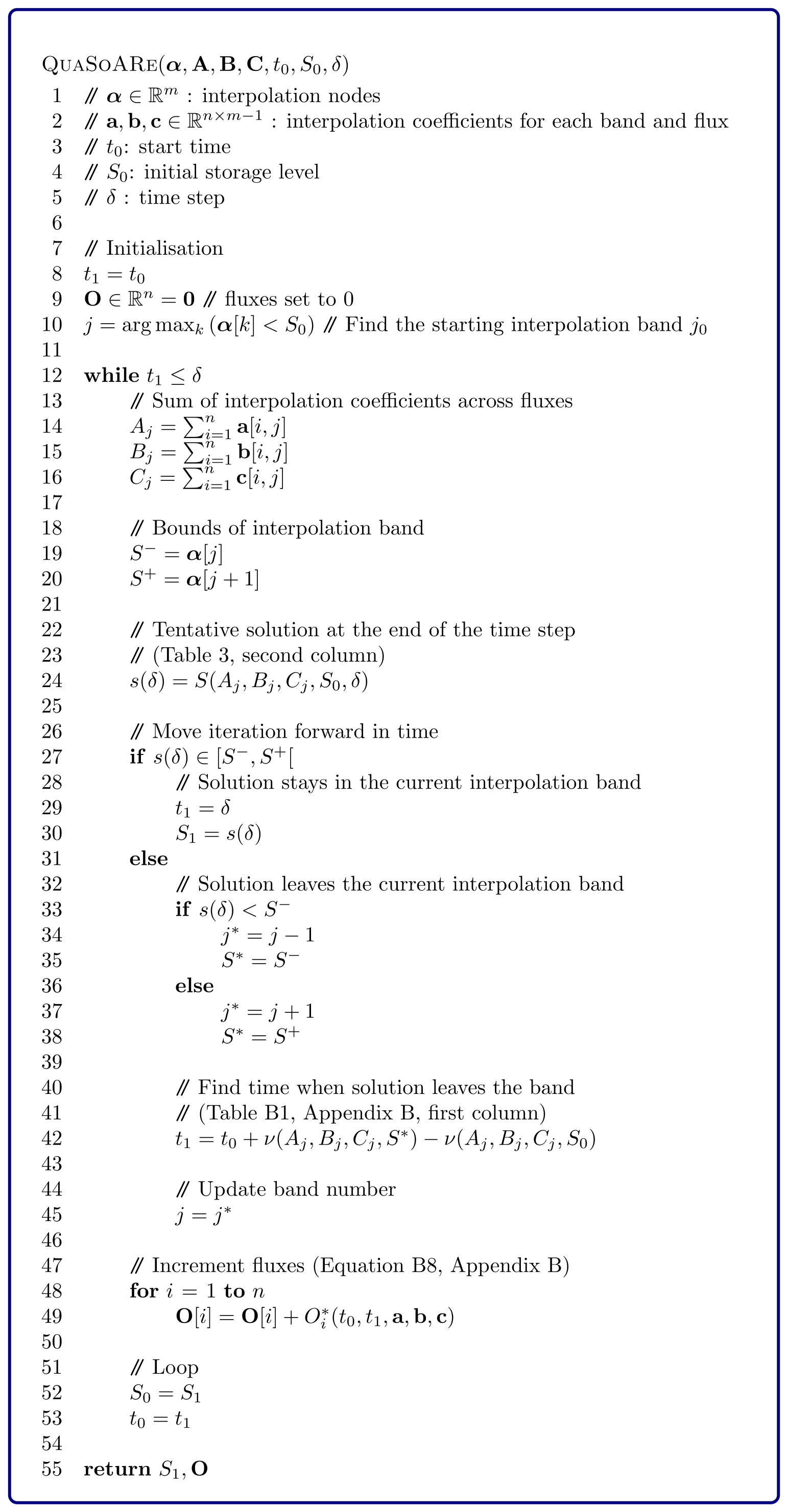
In summary, the solution presented in this section provides a way to solve an approximate reservoir equation where piecewise quadratic interpolations replace the original reservoir functions. The solution is fully analytical, including the computation of all reservoir fluxes. It can be implemented using the pseudo-code presented in Fig. 2. Alternatively, Lerat (2024) released an open-source software package where QuaSoARe is coded in both Python and C languages.

Figure 2 QuaSoARe pseudo-code.

3 Selecting interpolation nodes from the range of steady-state solutions

The QuaSoARe method presented in Sect. 2 relies on an interpolation of functions f_i using nodes ${\mathit{\alpha }}_j{\mathit{\}}}_{j=\mathrm{1},\mathrm{\dots },m}$. The choice of these nodes is crucial because it conditions the quality of the interpolation and, hence, the accuracy of the approximate solution. Let us now assume that the reservoir equation is solved for a fixed time step δ and a time series of p forcing values ${\left\{{\stackrel{\mathrm{̃}}{V}}_k\right\}}_{k=\mathrm{1},\mathrm{\dots }p}$. In most reservoirs used in hydrology, the reservoir equation has at least one steady-state solution for each time step k, denoted by ${\stackrel{\mathrm{‾}}{S}}_k$, that is a solution of

$$\begin{array}{}\text{(10)}& {\sum }_{i=\mathrm{1}}^n{f}_i\left({\stackrel{\mathrm{‾}}{S}}_k,{\stackrel{\mathrm{̃}}{V}}_k\right)=\mathrm{0}.\end{array}$$

If the set of all solutions ${\stackrel{\mathrm{‾}}{S}}_k$ is not empty, a simple approach is to set α₁ to $\min \left(\mathit{\right\{}{\stackrel{\mathrm{‾}}{S}}_k\mathit{\left\}}\right)$ and α_m to $\max \left(\mathit{\right\{}{\stackrel{\mathrm{‾}}{S}}_k\mathit{\left\}}\right)$. Subsequently, the α_i values are obtained by partitioning the interval [α₁, α_m] into m−1 equal sub-intervals. This approach relies on the fact that extreme values of s(t) are reached during time steps where the forcings ${\stackrel{\mathrm{̃}}{V}}_k$ are likely to be extremes. At the same time, steady-state solutions are storage values that are reached when the integration time step δ tends towards infinity. Consequently, when an extreme forcing value is used, a simulation run for an infinite time step is likely to result in storage values that are more extreme than any other values of s(t) seen when using a finite time step, hence constituting a conservative estimate for their bounds.

In addition, the steady-state solutions – and, hence, their range – are straightforward to compute with QuaSoARe because, if they exist, they are the roots of a quadratic polynomial (right-hand side of Eq. 9), which can be computed analytically from the coefficients A_j, B_j, and C_j. The corresponding functionality is included in the QuaSoARe software package (Lerat, 2024).

Unfortunately, the existence of steady-state solutions is not guaranteed for all reservoir equations. For example, the exponential reservoir with zero inflows does not have one (Michel et al., 2003). In cases like that, it is recommended that one use a trial-and-error approach to obtain a set of α_j values that cover the entire range of s(t) observed during the simulation.

4 Limitations of the method and recommendations

The QuaSoARe method is designed to solve a scalar ordinary differential equation. Hence, it cannot be used to solve a coupled system of equations. This is an important limitation of QuaSoARe as most hydrological models contain multiple stores that could benefit from a joint solution using a Runge–Kutta method, as presented by Clark and Kavetski (2010). Extension of QuaSoARe to higher dimensions is not straightforward because the analytical solutions underpinning the method do not have a vector equivalent. However, in the case where the model reservoirs operate in sequence with no feedback, a simple solution is to apply QuaSoARe to each reservoir in turn at a finer time interval than the desired time step. The fluxes generated at this finer time step can subsequently be used to feed the next reservoir in the model structure. This is arguably less efficient from a runtime perspective than applying QuaSoARe over the whole time step but is probably not dissimilar to discrete methods that often shorten the time step to very short sub-steps to control the error.

The second limitation of QuaSoARe is the quality of the piecewise quadratic interpolation. Figure 1 clearly shows that minor discrepancies between the true and interpolated flux functions can lead to noticeable simulation errors. The solution to this problem is to increase the number of interpolation nodes, as was shown in the illustrative example in Fig. 1, where the interpolation errors are reduced by a factor of 5 when switching from three to four nodes. This is straightforward to implement if a modeller starts with a high number of nodes, leading to an interpolation error smaller than their machine precision, as is done in Sect. 5. Such a small error level is theoretically achievable as the reservoir functions are assumed to be continuous and, hence, can be approximated up to any error level by a piecewise polynomial. If this configuration exceeds the modellers' runtime requirements then the number of nodes is progressively reduced to match this constraint.

Particular care should be taken with the interpolation of the reservoir function close to steady-state values discussed in the previous section. Functions with sharp transitions (e.g. rational fractions) cannot be interpolated accurately by a quadratic polynomial over large intervals. Consequently, if applied without constraint, the piecewise interpolation can overshoot and create erroneous steady-state values that do not exist in the original equation (i.e. values of S where $f_i^{\ast }\left(S,\stackrel{\mathrm{̃}}{V}\right)$ is null but not $f_i\left(S,\stackrel{\mathrm{̃}}{V}\right)$). To avoid this problem, a constraint is imposed in the computation of the interpolation coefficients presented in Appendix A to restrict the quadratic functions to be monotonic and to prevent them from crossing the 0 line if the original flux function did not.

Another limitation of QuaSoARe comes from the mathematical assumptions introduced in Sect. 1. More specifically, there is a need for flux functions to be Lipschitz continuous, which is equivalent to having bounded derivatives if the function is absolutely continuous. This assumption is required to ensure the unicity of the solutions of Eq. (1) and, hence, their monotonous nature, as demonstrated at the beginning of Sect. 2.2, but it eliminates many common flux functions encountered in hydrological systems (e.g. power functions of S with an exponent lower than 1). A first solution to this problem is to alter the flux functions to obtain smoother functions with bounded derivatives following Kavetski et al. (2006; see Sect. 5 of their paper) and, hence, to revert to the domain of applicability of QuaSoARe. If this is not an option, QuaSoARe may still generate reasonable simulations if the solution of Eq. (1) does not come close to any discontinuity in the flux function derivatives. This is, of course, case specific. An example of such a case is presented in the Supplement.

The discussion above highlights that QuaSoARe, like all numerical ODE solvers, is not guaranteed to converge for all reservoir equations and initial conditions. Reservoir equations often define stability regions where solutions starting from similar initial conditions remain close for all t>0. If the interpolation accuracy is low, it is possible that the approximate and original stability regions do not coincide. As a result, certain values of the initial conditions may lead to a stable solution for the original equation but not for QuaSoARe. Fortunately, this problem is related to interpolation accuracy and can be diagnosed before running QuaSoARe. Similarly to what is mentioned above, it is recommended that QuaSoARe is first run using a high number of interpolation nodes to ensure that stability regions are approximated accurately. Ultimately, the validity interval of the analytical solutions can be verified during QuaSoARe execution using the expressions given in Table B1. Consequently, it is possible to catch this type of problem before attempting a QuaSoARe iteration. Note that this case was never encountered in practice while running the tests presented in the following section, where QuaSoARe is applied to a range of non-linear reservoir models using challenging hydro-climate data.

5 Comparison of the method with alternative numerical schemes

5.1 Reservoir equations tested

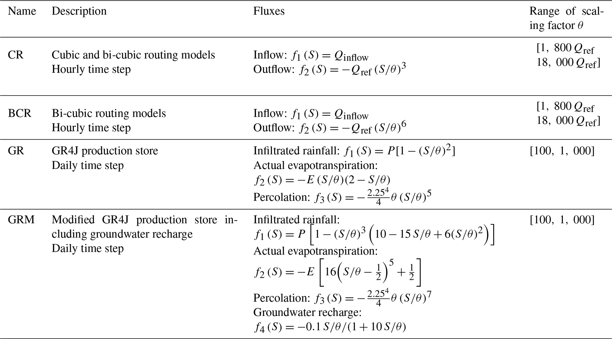
The QuaSoARe method is applied to four reservoir equations detailed in Table 1, representing common hydrological models of increasing complexity and non-linearity. All equations in this table depend on a storage scaling factor θ, which is expressed in the same unit as S. This factor acts like a storage capacity and controls the dynamic of the reservoir response. A total of 10 values of θ are evaluated for each equation using bounds for θ as indicated in the last column of Table 1.

The first two equations simulate the routing of an inflow time series from the upstream to downstream end of a river reach. This type of routing model is used in semi-distributed hydrological or flood forecasting models to approximate the solution of hydrodynamic equations (Hapuarachchi et al., 2022). The reach receives an inflow, denoted by Q_inflow(t), which is assumed to be fixed over the time step t. Outflow from the reach is computed as a power function of the reach storage following Yevdjevich (1959), where β is the power exponent multiplied by a reference flow, denoted by Q_ref, which is introduced to simplify dimensional analysis (see Table 1). The routing model is run at an hourly time step. The case where β=1 corresponds to the linear routing model (Meyer, 1941), while β=2 is the quadratic routing store solved analytically by Bentura and Michel (1997). Both cases can be treated as quadratic functions of the storage and, hence, can be solved exactly with QuaSoARe. To provide a more meaningful challenge for the method, the two cases where β=3 (cubic reservoir, denoted CR) and β=6 (bi-cubic reservoir, denoted BCR) are selected.

The third equation corresponds to the production store of the GR4J model (Perrin et al., 2003). This model is a well-established daily conceptual rainfall–runoff model used worldwide. Its production store, referred to as GR, receives rainfall (P) and potential evapotranspiration (E) and generates three fluxes: infiltrated rainfall into the store, actual evapotranspiration from the store, and percolation leaked from the store. The first two fluxes are quadratic functions of the store level, which could be solved exactly with QuaSoARe. However, the percolation flux introduces a strong non-linearity with a fifth-order polynomial. Note that the version of GR used in this paper computes the three fluxes simultaneously in a single equation, similarly to Santos et al. (2018), whereas they are solved sequentially using the operator-splitting method in the original GR4J model presented by Perrin et al. (2003).

The fourth equation, denoted GRM (GR modified), is inspired by the GR equation but increases the non-linearity of the fluxes by converting the infiltrated rainfall and the actual evapotranspiration to fifth-order polynomials. In addition, a fourth flux is added to represent groundwater recharge in the form of a rational fraction. Rational fractions are difficult to interpolate with polynomials as they possess asymptotes, which leads to a challenging case for QuaSoARe.

We highlight that the main objective of introducing these four reservoir equations is to obtain challenging tests for QuaSoARe that are representative of hydrological models in use. The aim is not to improve existing models such as GR4J or to reproduce accurately observed data from existing catchments. Consequently, one should not be surprised by the unusual formulation of certain equations in Table 1.

Table 1 Reservoir equations used for testing QuaSoARe.

5.2 Performance evaluation

The solution of the four reservoir equations is obtained with QuaSoARe using 5, 50, and 500 interpolation nodes. These three configurations lead to increasing accuracy of the interpolation of flux functions, which is expected to translate into higher solution accuracy.

QuaSoARe is compared with two discrete numerical schemes: the Radau IIA implicit Runge–Kutta method of order 5 (Hairer and Wanner, 1996), referred to as “Radau”, and the explicit Runge–Kutta method of order 5(4) (Dormand and Prince, 1980), denoted “RK45”. The Radau method was chosen because it is implicit (and, hence, is able to handle stiff equations) and of high order, with both characteristics leading us to qualify its outputs as the reference for comparison with other methods. The RK45 method was selected because it is the de facto explicit ODE solver that is widely recognised for its combination of speed and accuracy (Shampine, 2020). Both methods are run using the SciPy package implementation, where these two algorithms are coded in Python (Virtanen et al., 2020).

Three performance criteria are used to compare the performance of these integration methods. The first criterion measures the maximum absolute error between the fluxes computed from one of the methods above and the Radau method:

$$\begin{array}{}\text{(11)}& E^m=max\left\{\left|{\widehat{F}}_i^m\left(k\right)-{\widehat{F}}_i^{\mathrm{radau}}\left(k\right)\right|,k=\mathrm{1},\mathrm{\dots },p,i=\mathrm{1},\mathrm{\dots },n\right\},\end{array}$$

where ${\widehat{F}}_i^m\left(k\right)$ is the ith flux computed with method m for time step k. E^m is measured in the unit of the reservoir fluxes: m³ s⁻¹ for CR and BCR and mm d⁻¹ for the two remaining equations.

The second criterion is the maximum mass balance error between the fluxes computed with one of the methods and Radau:

$$\begin{array}{}\text{(12)}& B^m=max\left\{\left|{\displaystyle \frac{{\sum }_{k=\mathrm{1}}^p{\widehat{F}}_i^m\left(k\right)-{\widehat{F}}_i^{\mathrm{radau}}\left(k\right)}{{\sum }_{k=\mathrm{1}}^p{\widehat{F}}_i^{\mathrm{radau}}\left(k\right)}}\right|,i=\mathrm{1},\mathrm{\dots },n\right\}\times \mathrm{100}.\end{array}$$

B^m is dimensionless and reported in percent. Finally, the third criterion compares the runtime of a method against the Radau runtime:

$$\begin{array}{}\text{(13)}& R^m={\displaystyle \frac{T^m}{T^{\mathrm{radau}}}}\times \mathrm{100}.\end{array}$$

The runtime was measured on a laptop computer using a quad-core processor with a clock speed of 3 GHz. Note that the runtime of QuaSoARe is assessed using a version of the code written in pure Python so that it can be compared with the Radau and RK45 methods. A faster version of the code written in C within the same package is recommended for application purposes (Lerat, 2024). Measuring runtime is dependent on the machine used and thus may lack generality. An alternative metric to measure computational speed was tested (not reported here), where runtime is assessed by the number of flux function evaluations following Clark and Kavetski (2010). This metric provided similar results to R^m but is more challenging to interpret because QuaSoARe and the two discrete methods do not evaluate the same functions (analytical solutions for QuaSoARe and original flux functions for RK45 and Radau). Consequently, the simple runtime metric R^m is preferred here.

Table 2 Characteristic of the case study catchments.

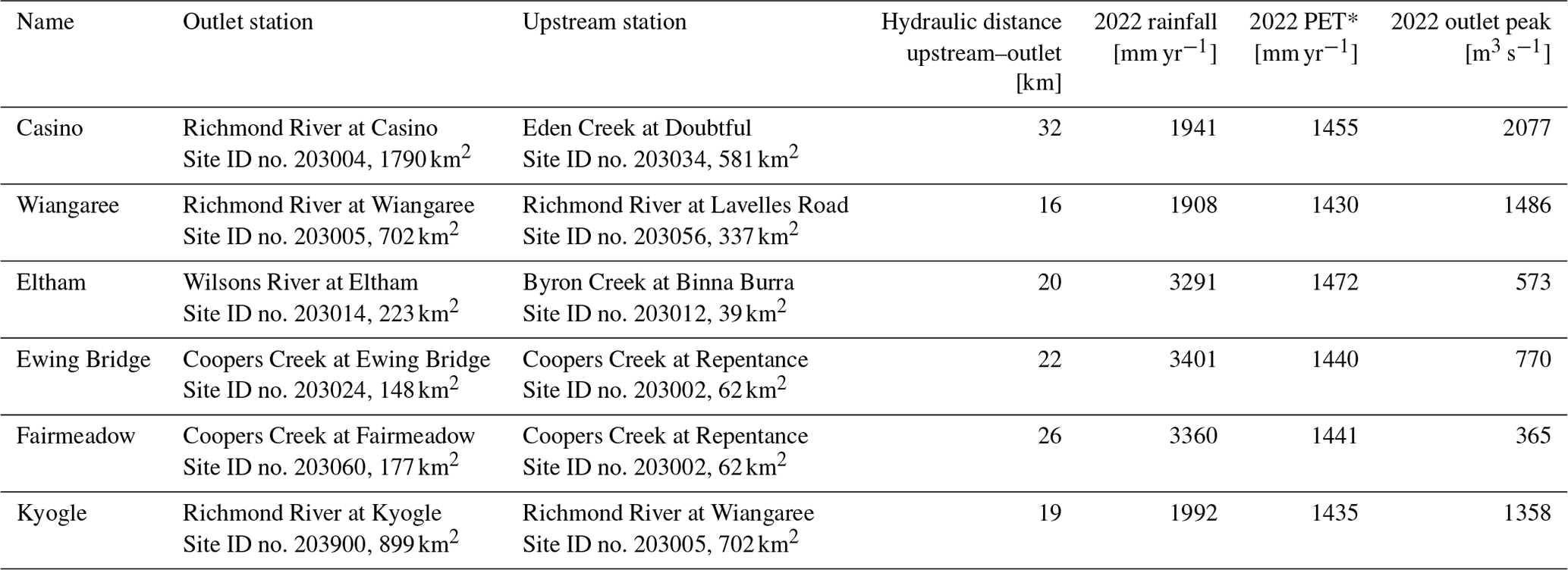
* Potential evapotranspiration

5.3 Case study area

QuaSoARe performance is evaluated for six sites in the Richmond River catchment in eastern Australia, close to the city of Lismore. The catchments are presented in Table 1, and their location is shown in Fig. 3. This area was chosen because it experienced a devastating flood in February 2022, which prompted an in-depth analysis of the event (Lerat et al., 2022). In addition, the maximum rainfall totals observed during this flood exceeded 700 mm in 24 h. Such extreme values constitute a challenging test for ODE solvers, as pointed out by La Follette et al. (2021). For each catchment, the outlet station and one station located upstream of the outlet, as shown in Fig. 3, are selected. The hourly streamflow data from 1 February 2022 to 10 April 2022 at the upstream station are used to run the two routing models (CR and BCR). The daily catchment average climate data from 1 January 2010 to 31 December 2022 are used to run the two hydrological models (GR and GRM).

As highlighted in Sect. 5.2, the aim of this paper is not to simulate hydrological processes accurately in these catchments but only to obtain realistic forcing data for the numerical experiments presented here.

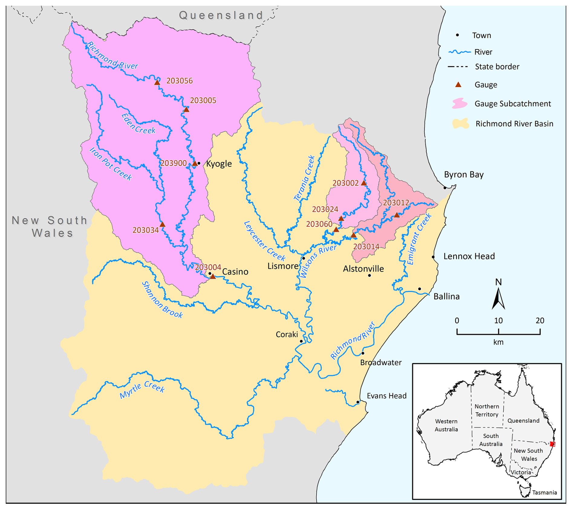
Figure 3 Location of the test catchments.

6 Results

6.1 Simulation of the GR4J production store

As an example of the application of QuaSoARe, this section details the results obtained with the GR4J production store (GR) presented in Table 1 for the Coopers Creek at Ewing Bridge catchment. The GR simulation is run with a storage scaling factor of 500 mm, a typical value for this parameter in Australia. Figure 4 shows the interpolation performed by QuaSoARe to approximate the three fluxes of the GR model using 10 nodes. The plots show the storage level S divided by the scaling factor θ on the x axis and the instantaneous flux on the y axis. The values for P and E required to compute the flux functions, as indicated in Table 1, are set to 4.2 and 3.1 mm d⁻¹, corresponding to the mean daily rainfall and potential evapotranspiration over the simulation period, respectively. The interpolation error is shown as a thin black line on the same plot using the a secondary y axis of a different scale. In the three plots, the QuaSoARe flux appears to be indistinguishable from the “true” flux, which is visually satisfying but insufficient to guarantee an accurate solution, as already seen in Fig. 1. The interpolation error for the first two fluxes is smaller in magnitude than $\mathrm{2}\times {\mathrm{10}}^{-\mathrm{15}}$ mm d⁻¹, which is comparable to the machine precision in most computers. This is expected as the first two GR flux functions are quadratic functions that can be interpolated exactly by QuaSoARe. Note that using 10 nodes is superfluous in this case as 2 nodes would suffice. The third flux is a power function with an exponent of 5, which cannot be interpolated exactly. Consequently, the interpolation error is larger, reaching a magnitude of up to $\mathrm{2.5}\times {\mathrm{10}}^{-\mathrm{3}}$ mm d⁻¹. This error remains small and shows an oscillating behaviour that is characteristic of polynomial interpolation using nodes with constant spacing. A potential improvement on this point is discussed in Sect. 7.

Figure 5 shows the daily storage levels and fluxes from the GR reservoir for the year 2022 using the Radau method (orange lines), considered to be the “truth”, and the QuaSoARe method (blue lines) configured with 10 interpolation nodes. In this figure, the Radau and QuaSoARe simulations are visually indistinguishable, which suggests that the interpolation errors shown in Fig. 4 remain small enough to have no lasting impact. The simulation errors are shown as thin black lines using a secondary y axis. These errors are lower in magnitude than $\mathrm{5}\times {\mathrm{10}}^{-\mathrm{3}}$ mm d⁻¹, which is negligible compared to typical errors of climate input data. Observation errors are rarely below 10⁻² mm d⁻¹ in a research catchment and are probably much higher in the study catchment considered here (e.g. Chubb et al., 2016, report root mean squared errors of gridded daily rainfall data above 4.5 mm d⁻¹). This result confirms that, despite the low number of nodes used, QuaSoARe can simulate the dynamic of the GR store and all its fluxes accurately. All flux errors exhibit oscillating patterns already noted in the interpolation error shown in Fig. 4c, which are likely to be due to a combination of oscillating interpolation errors and the alternation of wet and dry days leading to the sudden variations in actual evapotranspiration visible in Fig. 5c. This suggests that quantifying simulation errors in a highly non-linear reservoir equation is not straightforward and depends on both the quality of the numerical solution and the statistical characteristics of input forcings. More generally, the GR flux functions constitute a challenging case study because they combine the slow dynamic of the storage visible in Fig. 5a and the rapid changes in actual ET seen in Fig. 5c. QuaSoARe appears to resolve both with high accuracy.

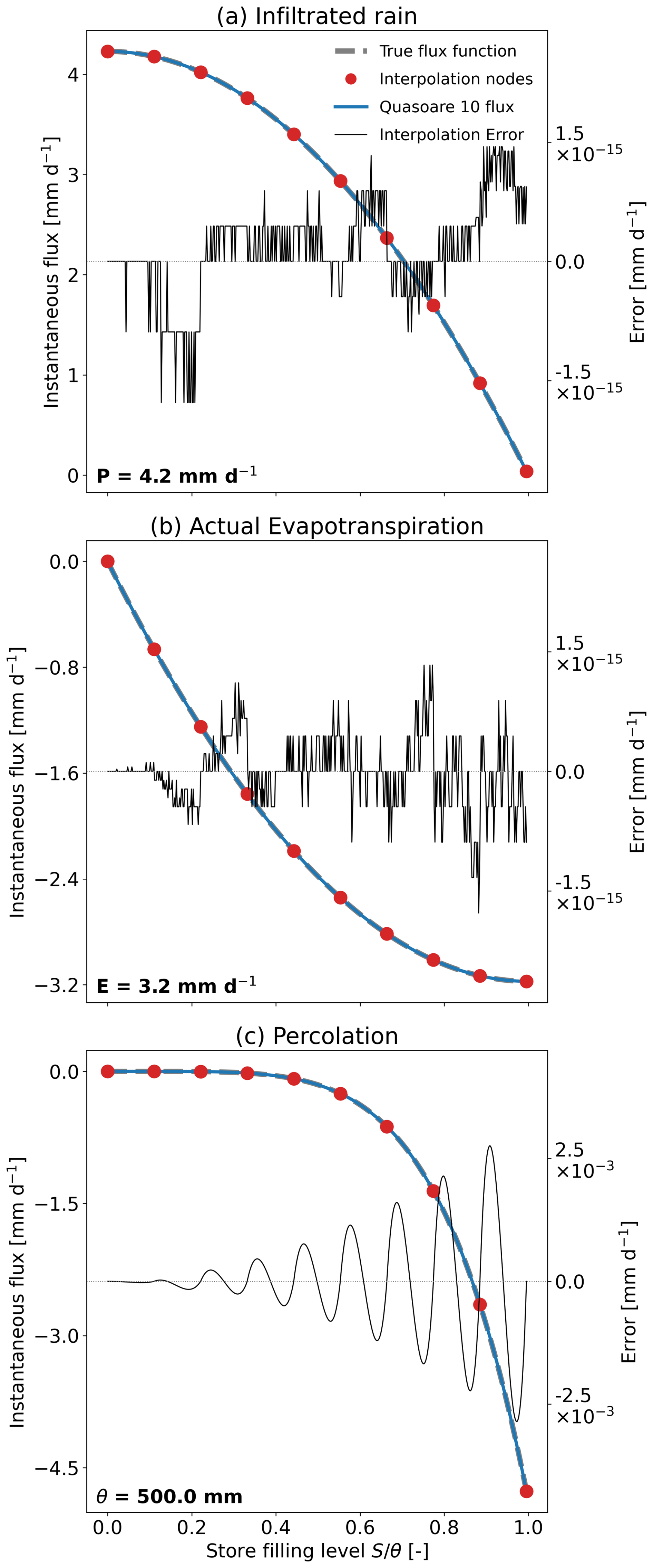
Figure 4 True and approximated flux functions of the GR reservoir equation with a scaling factor θ set to 500 mm. P and E variables are set to 4.2 and 3.1 mm, respectively, and QuaSoARe interpolation uses 10 nodes.

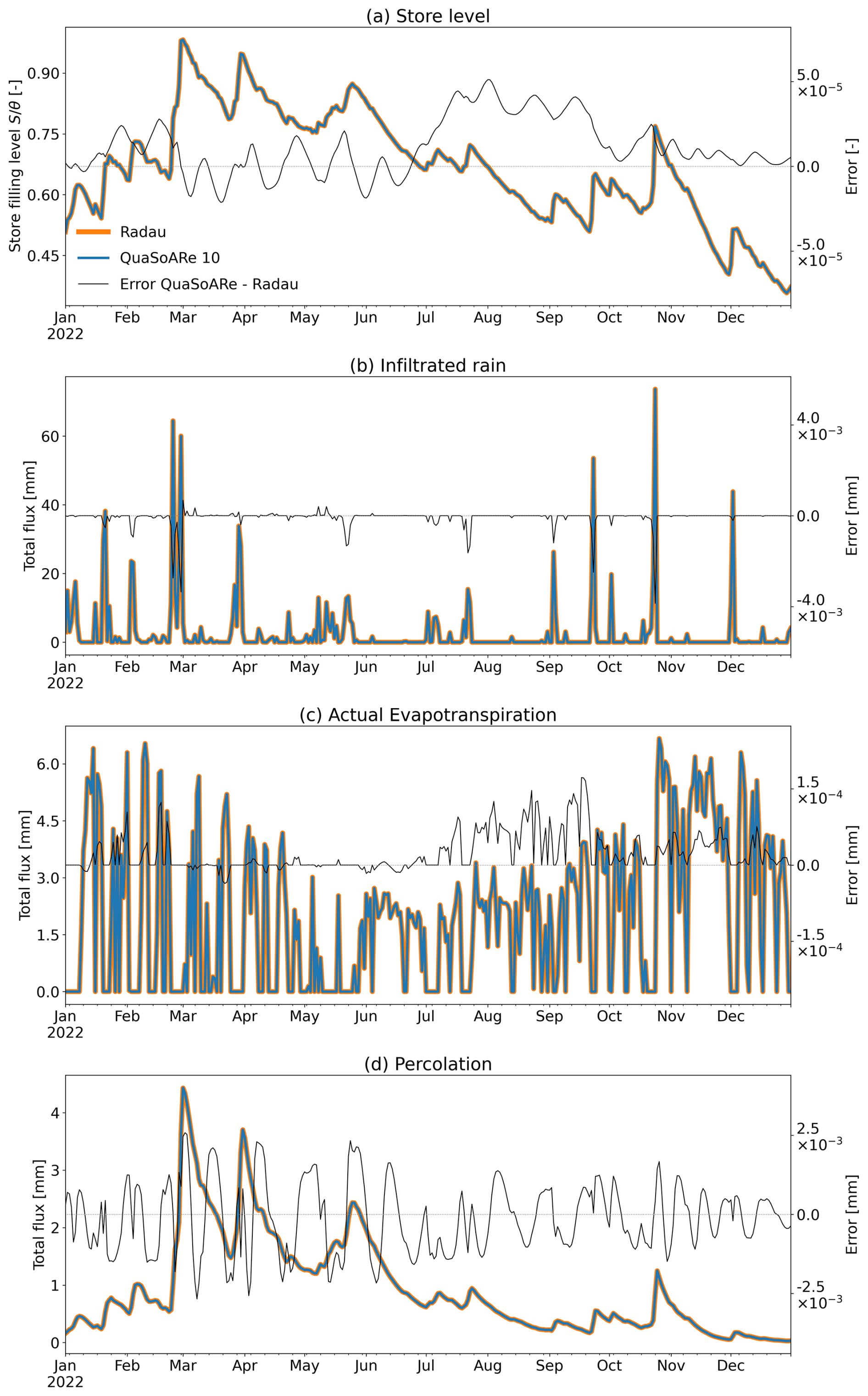
Figure 5 Radau and QuaSoARe storage level (a) and three fluxes (b–c) for the GR reservoir with a scaling factor θ set to 500 mm and using data from the Coopers Creek at Ewing Bridge catchment. QuaSoARe is configured with 10 interpolation nodes.

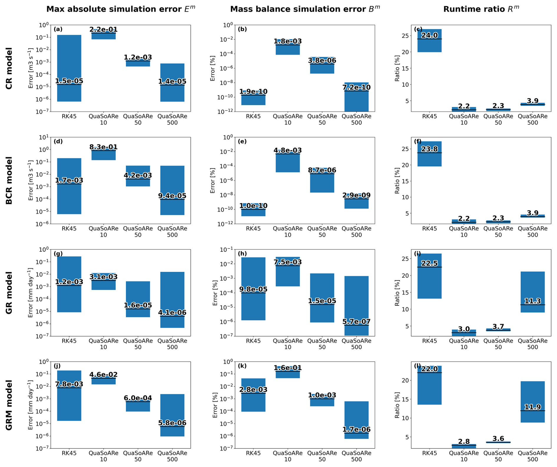
Figure 6 Comparison of performance metrics between the RK45 method and QuaSoARe using 10, 50, and 500 interpolation nodes. The Radau method is used as a reference simulation against which performance metrics are computed. Numbers in black denote the median value of the performance metric, while the blue boxes show their minimum–maximum range.

6.2 Performance assessment

Expanding the analysis of the previous section, Fig. 6 presents statistics of the three performance metrics introduced in Sect. 5.2. The metrics are computed for the four models (CR, BCR, GR, and GRM; see Table 1); the six study catchments (see Table 2); 10 values of the storage capacity parameter θ for each model (see Table 1); and five ODE solvers, including the Radau and RK45 methods and three configurations of QuaSoARe using 10, 50, and 500 nodes. Overall, 60 simulations are produced for each model and ODE solver combination. The Radau method is considered to be the reference against which the error of other methods is computed. The numbers shown in each plot of Fig. 6 report the median value of the metrics over the 60 corresponding simulations, while the blue boxes show their minimum–maximum range.

All the plots in Fig. 6 reveal that QuaSoARe simulations are extremely close to the Radau outputs if QuaSoARe is configured with a high number of nodes (500). The median absolute simulation error of QuaSoARe (E^m) varies between $\mathrm{4.4}\times {\mathrm{10}}^{-\mathrm{6}}$ mm d⁻¹ for the GR model (Fig. 6g) to $\mathrm{9.4}\times {\mathrm{10}}^{-\mathrm{5}}$ m³ s⁻¹ for the BCR model. Both values are several orders of magnitude lower than the observation errors, which means that simulations from QuaSoARe and Radau can be considered to be interchangeable from a modeller's perspective. Importantly, these results also hold for the mass balance metric B^m, where the average difference between the flux totals from QuaSoARe and Radau remains lower than $\mathrm{2}\times {\mathrm{10}}^{-\mathrm{6}}$ % (Fig. 6k). At the same time, the QuaSoARe runtime is only a fraction of the Radau runtime, with median values varying from 3.8 % for the CR and BCR models (Fig. 6c and f) to 11.8 % for GRM (Fig. 6l). Finally, QuaSoARe performance is better than RK45 for most models and performance metrics. For example, the maximum absolute error of QuaSoARe is several orders of magnitude lower than that of RK45, except for the CR model, where the error of both methods is close to $\mathrm{1.5}\times {\mathrm{10}}^{-\mathrm{5}}$ m³ s⁻¹ (Fig. 6a).

When fewer nodes are used, the errors of QuaSoARe increase and worsen the performance metrics. For example, the median maximum error for the GR model, shown in Fig. 6g, increases from $\mathrm{4.1}\times {\mathrm{10}}^{-\mathrm{6}}$ m³ s⁻¹ when using 500 nodes to $\mathrm{3.1}\times {\mathrm{10}}^{-\mathrm{3}}$ m³ s⁻¹ when using 10 nodes. This degradation is expected as the interpolation of the reservoir functions worsens with fewer nodes. Nonetheless, the errors remain insignificant compared to observation errors, which suggests that a low number of nodes remains an attractive configuration when applying QuaSoARe to hydrological models. The runtime efficacy of QuaSoARe when using 10 nodes is noticeable, with values remaining lower than 3 % of the Radau runtime for the four models.

We highlight that the results presented here correspond to challenging test cases with highly non-linear flux functions. For example, the GRM reservoir includes functions with polynomials of up to order 7. In addition, the selected catchments exhibit a particularly challenging hydro-climate regime to simulate, with maximum rainfall intensity exceeding several hundred millimetres per day.

7 Discussion

The QuaSoARe method presented in this paper is a valuable alternative to existing numerical schemes for solving the scalar reservoir equation for three reasons. First, the algorithm is simple to understand and code, relying, essentially, on the interpolation of the reservoir functions by piecewise quadratic polynomials. Consequently, it is believed to be straightforward to integrate into an existing modelling platform, and it helps strengthen the numerical solution of hydrological models without adding a significant burden in terms of code maintenance. Second, the method is much faster than standard alternatives such as the RK45 (explicit) and Radau (implicit) schemes tested in this paper. QuaSoARe reduces the runtime by a factor of 20 to 50 compared to Radau, depending on the model. This point further reinforces the value of the method for hydrological modelling tasks requiring repeated model evaluation, such as automated calibration or data assimilation. Finally, the configuration of QuaSoARe can be modified simply by changing the number of interpolation nodes to vary between highly accuracy but slow simulation times (say, with 500 nodes) to lower accuracy and fast runtime (say, with 10 nodes). As a result, the modeller remains in control of the algorithm via a single and easily interpretable configuration parameter.

The QuaSoARe performance reported in this paper is satisfactory, but one may wonder if there could be ways to improve it further without changing the algorithm's core. The first point that could be improved is the quality of the interpolation. Our method relies on piecewise quadratic polynomials, which could be replaced by more flexible functions. However, the requirements of QuaSoARe in terms of interpolation functions are stringent because they should, at the same time, be stable by linear combination (to compute all fluxes) and should lead to an analytical solution of the approximate reservoir equation. A powerful alternative to the quadratic polynomials explored in early versions of this work is a combination of exponential functions. This choice was later abandoned because it was prone to numerical overflow and did not provide significant performance improvements. Nonetheless, it is believed that other functions could meet the QuaSoARe requirements and help improve its performance in difficult situations, such as when the flux functions are rational fractions, which are notoriously tough to interpolate with polynomials (Berrut and Trefethen, 2004).

Related to this point, one may wonder about the performance of a linear interpolation in comparison to its quadratic counterpart as presented in this paper. Tests not shown here revealed that the linear interpolation worsens the maximum absolute error by an approximate factor of 10 with a similar runtime. Interestingly, the difference between the two approaches seems to persist even when using a large number of nodes and, hence, when the interpolation of both the linear and quadratic is expected to be close. Overall, the quadratic interpolation is recommended, but the linear approach as a degraded functionality is kept in the code (Lerat, 2024).

Several ideas could be explored to improve QuaSoARe further. In this paper, the interpolation nodes are placed at equal intervals between the two extremes α₁ and α_m. This could easily be modified to find the nodes providing the lowest interpolation errors. This might reduce the oscillations of the interpolation errors visible in Fig. 4c. However, this would also increase the algorithm's complexity, whereas simplicity was favoured in this first version of QuaSoARe. Finally, it is flagged that this method could be combined with a discrete method in a way similar to the exponential-integrator approach of Pope (1963). This will likely improve performance further but will also require using a discrete method, which was discarded in this paper's Introduction. However, this could be an interesting avenue for a modeller familiar with discrete methods.

Beyond potential improvements in QuaSoARe, we highlight that the flux functions defined in an empirical modelling context, like most rainfall–runoff models, remain arbitrary and are not derived from physically based equations. In this case, one could argue that piecewise quadratic functions could themselves constitute valid flux functions. This approach would have two merits: first, the instantaneous model equations could be characterised by a small set of coefficients (the interpolation coefficients), hence becoming fully parametric and amenable to optimisation or data assimilation, and, second, the model could be solved exactly with QuaSoARe. As a result, models formulated in this way could become powerful components of flexible modelling environments. This avenue is currently being explored to extend the work of Lerat et al. (2024), in which improvement of the model structure is obtained by updating state equations via data assimilation methods.

8 Conclusion

This paper presents a simple numerical algorithm called QuaSoARe to solve the instantaneous reservoir equation, provide a basis for building hydrological models based on this equation, and generate fast and accurate simulations. The method was tested on a range of highly non-linear models that are representative of hydrological models in use. Its performance suggests that the method matches the accuracy of a high-order implicit discrete method while requiring a fraction of its runtime. Yet, the method algorithm is simple and can be described with a short pseudo-code, which is included in this paper.

The method is limited by its applicability to scalar equations and by the quality of the quadratic interpolation underlying its analytical solution. To model a series of reservoirs, the implementation of sub-time-step integration is suggested. Higher accuracy in the interpolation of reservoir functions can always be achieved by increasing the number of interpolation nodes. The results of this study showed that using 10 to 50 nodes leads to an accuracy level that is an order of magnitude smaller than the typical error in hydro-climate observation data.

Appendix A: Interpolation coefficients

For each function f_i and each interval $[{\mathit{\alpha }}_j,{\mathit{\alpha }}_{j+\mathrm{1}}]$, the interpolation process requires values of the coefficients a_i,j, b_i,j, and c_i,j so that the approximated function $f_i^{\ast }$ matches f_i as best as possible. This is achieved by matching f_i at the two points α_j and α_j+1 and at their midpoint. Assuming that ${\mathit{\alpha }}_j<{\mathit{\alpha }}_{j+\mathrm{1}}$, the quadratic interpolation leads to

$$\begin{array}{}\text{(A1)}& {\displaystyle }{a}_{i,j}={\displaystyle \frac{\mathrm{2}{f}_{\mathrm{0}}+\mathrm{2}{f}_{\mathrm{1}}-\mathrm{4}{f}_m}{{\left({\mathit{\alpha }}_{j+\mathrm{1}}-{\mathit{\alpha }}_j\right)}^{\mathrm{2}}}},\text{(A2)}& {\displaystyle }{b}_{i,j}=-\mathrm{2}{\mathit{\alpha }}_j{a}_{i,j}+{\displaystyle \frac{\mathrm{4}{f}_m-\mathrm{3}{f}_{\mathrm{0}}-f_{\mathrm{1}}}{{\mathit{\alpha }}_{j+\mathrm{1}}-{\mathit{\alpha }}_j}},\text{(A3)}& {\displaystyle }{c}_{i,j}={\mathit{\alpha }}_j^{\mathrm{2}}{a}_{i,j}-{\mathit{\alpha }}_j{\displaystyle \frac{\mathrm{4}{f}_m-\mathrm{3}{f}_{\mathrm{0}}-f_{\mathrm{1}}}{{\mathit{\alpha }}_{j+\mathrm{1}}-{\mathit{\alpha }}_j}}+f_{\mathrm{0}},\end{array}$$

where

$$\begin{array}{}\text{(A4)}& f_{\mathrm{0}}=f_i\left({\mathit{\alpha }}_j\right),f_{\mathrm{1}}=f_i\left({\mathit{\alpha }}_{j+\mathrm{1}}\right),f_m=f_i\left({\displaystyle \frac{{\mathit{\alpha }}_j+{\mathit{\alpha }}_{j+\mathrm{1}}}{\mathrm{2}}}\right).\end{array}$$

This solution is straightforward but can lead to a function $f_i^{\ast }$ that is non-monotonous, for example, when interpolating a function f_i that presents sharp transitions or asymptotes. This situation can create an issue related to the steady-state solution of Eq. (1), as discussed in Sect. 4. To avoid this undesirable effect, the value of f_m used in Eqs. (A1) to (A3) is replaced by a value $f_m^{\ast }$ defined as follows:

$$\begin{array}{}\text{(A5)}& f_m^{\ast }=\max (f_m^{-},min\left(f_m^{+},f_m\right)),\end{array}$$

where the two bounds $f_m^{-}$ and $f_m^{+}$ are given by

$$\begin{array}{}\text{(A6)}& {\displaystyle }{f}_m^{-}=min\left({\displaystyle \frac{\mathrm{3}{f}_{\mathrm{0}}+f_{\mathrm{1}}}{\mathrm{4}}},{\displaystyle \frac{f_{\mathrm{0}}+\mathrm{3}{f}_{\mathrm{1}}}{\mathrm{4}}}\right),\text{(A7)}& {\displaystyle }{f}_m^{+}=max\left({\displaystyle \frac{\mathrm{3}{f}_{\mathrm{0}}+f_{\mathrm{1}}}{\mathrm{4}}},{\displaystyle \frac{f_{\mathrm{0}}+\mathrm{3}{f}_{\mathrm{1}}}{\mathrm{4}}}\right).\end{array}$$

It can be verified that using $f_m^{\ast }$ instead of f_m in Eqs. (A1) to (A3) leads to a monotonous quadratic function $f_i^{\ast }$.

Appendix B: Analytical solution of the approximated reservoir equation

In this Appendix, the approximate reservoir equation (Eq. 9) is solved over an interval [t₀, t₁] such that $\forall t,S\left(t\right)\in \left[{\mathit{\alpha }}_j{\mathit{\alpha }}_{j+\mathrm{1}}\right]$, starting from the initial condition S(t₀)=S₀. This solution is obtained by separating the variables leading to the following integral equation:

$$\begin{array}{}\text{(B1)}& \underset{S_{\mathrm{0}}}{\overset{S_{\mathrm{1}}}{\int }}{\displaystyle \frac{\mathrm{d}S}{A_j{S}^{\mathrm{2}}+B_{j}S+C_j}}=t,\end{array}$$

where S₁=S(t₁). Here, it is assumed that either A_j≠0 or B_j≠0. If this is not the case, the interpolation function $f_i^{\ast }$ is simply the constant C_j, leading to

Table B1 Solutions of approximate reservoir equation.

$$\begin{array}{}\text{(B2)}& S\left(t_{\mathrm{1}}\right)=S_{\mathrm{0}}+C_j\mathit{\tau },\end{array}$$

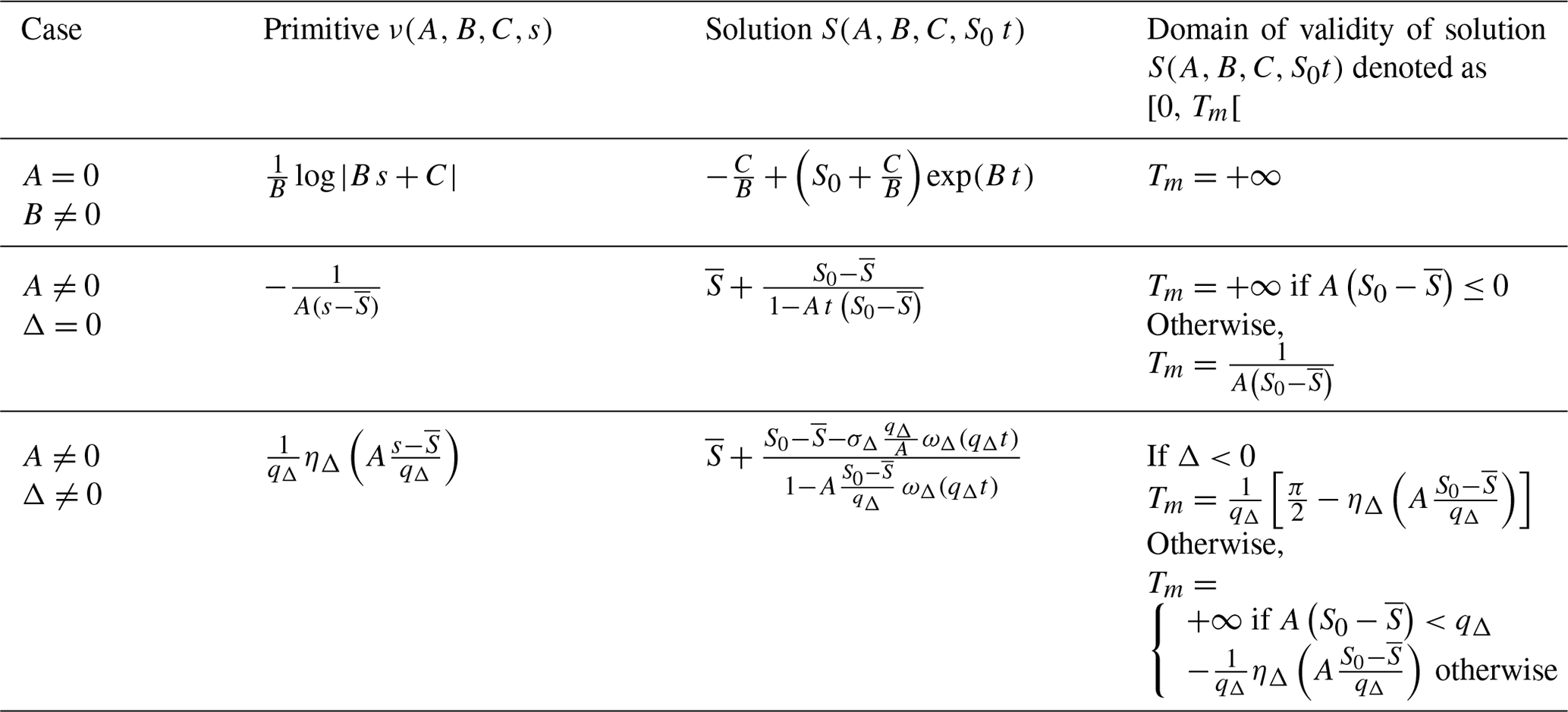
where $\mathit{\tau }=t_{\mathrm{1}}-t_{\mathrm{0}}$. If A_j≠0 or B_j≠0, the solutions of Eq. (B1) can be obtained from any calculus textbook. They are presented succinctly in Table B1. In this table, the subscript j is dropped to simplify notations. The function ν mentioned in the second column of Table B1 is defined as the following primitive:

$$\begin{array}{}\text{(B3)}& \mathit{\nu }\left(A_j,B_j,C_j,s\right)=\int {\displaystyle \frac{\mathrm{d}S}{A_j{S}^{\mathrm{2}}+B_{j}S+C_j}}.\end{array}$$

This function is used to compute the times t_l and t_u mentioned in cases 2 and 3 in Sect. 2.3.

In Table B1, the following expressions are used to simplify notations further:

$$\begin{array}{}\text{(B4)}& {\displaystyle }\stackrel{\mathrm{‾}}{S}=-{\displaystyle \frac{B_j}{\mathrm{2}{A}_j}},\text{(B5)}& {\displaystyle }\mathrm{\Delta }=B_j^{\mathrm{2}}-\mathrm{4}{A}_j{C}_j,{\mathit{\sigma }}_{\mathrm{\Delta }}=\text{sgn}\left(\mathrm{\Delta }\right),q_{\mathrm{\Delta }}={\displaystyle \frac{\sqrt{\left|\mathrm{\Delta }\right|}}{\mathrm{2}}},\text{(B6)}& {\displaystyle }{\mathit{\omega }}_{\mathrm{\Delta }}\left(x\right)=\left\{\begin{array}{ll}\tan \left(x\right)& \text{ if }\mathrm{\Delta }<\mathrm{0}\\ \text{tanh}\left(x\right)& \text{ if }\mathrm{\Delta }>\mathrm{0}\end{array},\right.\text{(B7)}& {\displaystyle }{\mathit{\eta }}_{\mathrm{\Delta }}\left(x\right)=\left\{\begin{array}{lll}\text{atan}\left(x\right)& \text{ if }\mathrm{\Delta }<\mathrm{0}& \\ -\text{atanh}\left(x\right)& \text{ if }\mathrm{\Delta }>\mathrm{0}& \text{ and }\left|x\right|<\mathrm{1}\\ -\text{atanh}\left(\mathrm{1}/x\right)& \text{ if }\mathrm{\Delta }>\mathrm{0}& \text{ and }\left|x\right|>\mathrm{1}\end{array},\right.\end{array}$$

where sgn(Δ) is equal to +1 if Δ≥0 and to −1 otherwise.

Focus is now given to finding an expression for the total of the ith flux introduced in Eq. (2). Combining the solution of Eq. (B1) given in the third column of Table B1, denoted S(t), with Eq. (2) gives

$$\begin{array}{}\text{(B8)}& \begin{array}{rl}{O}_i^{\ast }(t_{\mathrm{0}},t_{\mathrm{1}})& =\underset{t_{\mathrm{0}}}{\overset{t_{\mathrm{1}}}{\int }}{f}_i^{\ast }\left(S\left(t\right)\right)\mathrm{d}t\\ & =a_{i,j}\underset{t_{\mathrm{0}}}{\overset{t_{\mathrm{1}}}{\int }}S(t{)}^{\mathrm{2}}\mathrm{d}t+b_{i,j}\underset{t_{\mathrm{0}}}{\overset{t_{\mathrm{1}}}{\int }}S(t)\mathrm{d}t+c_{i,j}\mathit{\tau }\end{array},\end{array}$$

where $\mathit{\tau }=t_{\mathrm{1}}-t_{\mathrm{0}}$. Note that, in the above equations, the integral boundaries used in Eq. (2) ([0,δ]) are generalised to [t₀, t₁] because fluxes are often computed on an smaller interval than [0, δ] in the algorithm described in Sect. 2.3. Solving Eq. (B8) is equivalent to integrating S(t) and S(t)² between t₀ and t₁. To compute these two integrals, different cases for A_j and B_j are considered, starting with $A_j=B_j=\mathrm{0}$. In this case, the following is obtained from Eq. (B2):

$$\begin{array}{}\text{(B9)}& {\displaystyle }\underset{t_{\mathrm{0}}}{\overset{t_{\mathrm{1}}}{\int }}S\left(t\right)\mathrm{d}t=S_{\mathrm{0}}\mathit{\tau }+C_j{\displaystyle \frac{{\mathit{\tau }}^{\mathrm{2}}}{\mathrm{2}}},\text{(B10)}& {\displaystyle }\underset{t_{\mathrm{0}}}{\overset{t_{\mathrm{1}}}{\int }}S(t{)}^{\mathrm{2}}\mathrm{d}t=S_{\mathrm{0}}^{\mathrm{2}}\mathit{\tau }+S_{\mathrm{0}}{C}_j{\mathit{\tau }}^{\mathrm{2}}+C_j^{\mathrm{2}}{\displaystyle \frac{{\mathit{\tau }}^{\mathrm{3}}}{\mathrm{3}}}.\end{array}$$

It is now assumed that A_j=0 and B_j≠0. The two integrals can be obtained by manipulating and integrating Eq. (9) as follows:

$$\begin{array}{}\text{(B11)}& {\displaystyle }\begin{array}{rl}\underset{t_{\mathrm{0}}}{\overset{t_{\mathrm{1}}}{\int }}{\displaystyle \frac{\mathrm{d}S}{\mathrm{d}t}}\mathrm{d}t& =B_j\underset{t_{\mathrm{0}}}{\overset{t_{\mathrm{1}}}{\int }}S\left(t\right)\mathrm{d}t+C_j\mathit{\tau }\\ & \Rightarrow \underset{t_{\mathrm{0}}}{\overset{t_{\mathrm{1}}}{\int }}S\left(t\right)\mathrm{d}t={\displaystyle \frac{\mathrm{1}}{B_j}}(S_{\mathrm{1}}-S_{\mathrm{0}}-C_j\mathit{\tau }),\end{array}\text{(B12)}& {\displaystyle }\begin{array}{rl}& \underset{t_{\mathrm{1}}}{\overset{t_{\mathrm{2}}}{\int }}S\left(t\right){\displaystyle \frac{\mathrm{d}S}{\mathrm{d}t}}\mathrm{d}t=B_j\underset{t_{\mathrm{1}}}{\overset{t_{\mathrm{2}}}{\int }}S{\left(t\right)}^{\mathrm{2}}\mathrm{d}t+C_j\underset{t_{\mathrm{1}}}{\overset{t_{\mathrm{2}}}{\int }}S\left(t\right)\mathrm{d}t\\ & \Rightarrow \underset{t_{\mathrm{0}}}{\overset{t_{\mathrm{1}}}{\int }}S(t{)}^{\mathrm{2}}\mathrm{d}t={\displaystyle \frac{\mathrm{1}}{B_j}}\left({\displaystyle \frac{S_{\mathrm{1}}^{\mathrm{2}}-S_{\mathrm{0}}^{\mathrm{2}}}{\mathrm{2}}}-C_j\underset{t_{\mathrm{0}}}{\overset{t_{\mathrm{1}}}{\int }}S\left(t\right)\mathrm{d}t\right).\end{array}\end{array}$$

With these two equations, integrating S is done first using Eq. (B11). This integral is then used in Eq. (B13) to compute the integral of S².

Finally, the general case where A_j≠0 is addressed. Following a similar approach than above, Eq. (9) is rearranged and integrated as follows:

$$\begin{array}{}\text{(B13)}& \begin{array}{rl}& \underset{t_{\mathrm{0}}}{\overset{t_{\mathrm{1}}}{\int }}{\displaystyle \frac{\mathrm{d}S}{\mathrm{d}t}}\mathrm{d}t=A_j\underset{t_{\mathrm{0}}}{\overset{t_{\mathrm{1}}}{\int }}S(t{)}^{\mathrm{2}}\mathrm{d}t+B_j\underset{t_{\mathrm{0}}}{\overset{t_{\mathrm{1}}}{\int }}S(t)\mathrm{d}t+C_j\mathit{\tau }\\ & \Rightarrow \underset{t_{\mathrm{0}}}{\overset{t_{\mathrm{1}}}{\int }}S(t{)}^{\mathrm{2}}\mathrm{d}t={\displaystyle \frac{\mathrm{1}}{A_j}}\left(S_{\mathrm{1}}-S_{\mathrm{0}}-B_j\underset{t_{\mathrm{0}}}{\overset{t_{\mathrm{1}}}{\int }}S\left(t\right)\mathrm{d}t-C_j\mathit{\tau }\right).\end{array}\end{array}$$

Consequently, the integration of S² can be deduced from the one of S. For the integration of S, the expression of S(t) given in the third column of Table B1 is used. If Δ=0 (see row before last in Table B1), the following is obtained:

$$\begin{array}{}\text{(B14)}& \underset{t_{\mathrm{0}}}{\overset{t_{\mathrm{1}}}{\int }}S\left(t\right)\mathrm{d}t=\stackrel{\mathrm{‾}}{S}\mathit{\tau }-{\displaystyle \frac{\mathrm{1}}{a}}\log \left[\mathrm{1}-a\mathit{\tau }\left(S_{\mathrm{0}}-\stackrel{\mathrm{‾}}{S}\right)\right].\end{array}$$

A value Δ≠0 leads to (see last row in Table B1)

$$\begin{array}{}\text{(B15)}& \begin{array}{rl}\underset{t_{\mathrm{0}}}{\overset{t_{\mathrm{1}}}{\int }}S\left(t\right)\mathrm{d}t& =\stackrel{\mathrm{‾}}{S}\mathit{\tau }+{\displaystyle \frac{\mathrm{1}}{\mathrm{2}a}}\log \left(\mathrm{1}-{\mathit{\sigma }}_{\mathrm{\Delta }}{\mathit{\omega }}_{\mathrm{\Delta }}^{\mathrm{2}}\left(q_{\mathrm{\Delta }}\mathit{\tau }\right)\right)\\ & -{\displaystyle \frac{\mathrm{1}}{a}}\log \left(\mathrm{1}-a{\displaystyle \frac{S_{\mathrm{0}}-\stackrel{\mathrm{‾}}{S}}{q_{\mathrm{\Delta }}}}{\mathit{\omega }}_{\mathrm{\Delta }}\left(q_{\mathrm{\Delta }}\mathit{\tau }\right)\right).\end{array}\end{array}$$