Synchronization frequency analysis and stochastic simulation of multi-site flood flows based on the complicated vine copula structure

Accurately modeling and predicting flood flows across multiple sites within a watershed presents significant challenges due to potential issues of insufficient accuracy and excessive computational demands in existing methodologies. In response to these challenges, this study introduces a novel approach centered around the use of vine copula models, termed RDV-Copula (reduced-dimension vine copula construction approach). The core of this methodology lies in its ability to integrate and extract complex data before constructing the copula function, thus preserving the intricate spatial–temporal connections among multiple sites while substantially reducing the vine copula's complexity. This study performs a synchronization frequency analysis using the devised copula models, offering valuable insights into flood encounter probabilities. Additionally, the innovative approach undergoes validation by comparison with three benchmark models which vary in dimensions and nature of variable interactions. Furthermore, the study conducts stochastic simulations, exploring both unconditional and conditional scenarios across different vine copula models. Applied in the Shifeng Creek watershed, China, the findings reveal that vine copula models are superior in capturing complex variable relationships, demonstrating significant spatial interconnectivity crucial for flood risk prediction in heavy-rainfall events. Interestingly, the study observes that expanding the model's dimensions does not inherently enhance simulation precision. The RDV-Copula method not only captures comprehensive information effectively but also simplifies the vine copula model by reducing its dimensionality and complexity. This study contributes to the field of hydrology by offering a refined method for analyzing and simulating multi-site flood flows.

1 Introduction

Floods are the most frequent natural disaster, inflicting substantial economic losses, environmental degradation, and human casualties (Teng et al., 2017). As reported by Centre for Research on the Epidemiology of Disasters (CRED), floods represented 45.6 % of worldwide natural disasters in 2022, affecting an average of 57.1 million people annually (CRED, 2023). The data also indicated a 4.76 % increase in flood occurrences in 2022 compared to the annual average from 2002 to 2021 (CRED, 2023). Therefore, it is very meaningful and essential to analyze flooding and achieve flood risk control. At the watershed scale, flood risk is primarily influenced by rainfall patterns and interconnections among sub-watersheds. Large floods often result from the merging of floods from multiple sub-watersheds (Prohaska and Ilic, 2010). Concurrent flood events cause runoff from various sources to merge, forming large floods that pose threats to downstream regions. As a result, analyzing the runoff at various sites not only provides a better understanding of the flood characteristics within the watershed but also contributes to the development of flood control programs to avoid flood risks.

There are currently many techniques for analyzing hydrological variables. Common univariate methods include statistical analyses such as frequency analysis (Stedinger et al., 1993), extreme value theory (Coles, 2001), and time series analysis methods like the autoregressive integrated moving average (ARIMA) model (Box and Jenkins, 2013). However, univariate analyses often fall short in accurately estimating the risks associated with extreme events due to their inability to account for the interdependence of variables (Guo et al., 2023; Khan et al., 2023). This oversight can lead to a significant underestimation or overestimation of risks, particularly given the inherent relationships among variables within a catchment. To address the complexity of these relationships across multiple variables, researchers have turned to multivariate analysis techniques. Methods such as autoregressive (AR) models are utilized for analyzing temporal correlations (Box and Jenkins, 2013), while spatial relationships can be examined using techniques like geostatistical methods (Isaaks and Srivastava, 1989), spatial regression models (Bekker et al., 2001), copula functions (Sklar, 1959), and Bayesian hierarchical models (Gelman et al., 2013). However, these methods have their limitations. AR models, while effective for temporal analysis, do not account for spatial dependencies. Geostatistical methods and spatial regression models focus primarily on spatial relationships but may struggle with temporal dynamics. Bayesian hierarchical models can handle complex dependencies but often involve high computational demands and require substantial prior information. In contrast, copula functions offer substantial advantages when dealing with multivariate spatial–temporal relationships. They provide a flexible framework for modeling dependencies between variables without assuming a specific marginal distribution, allowing for a more accurate representation of complex interdependencies. Later adopted in hydrology by De Michele and Salvadori (2003), copula functions link multi-dimensional probability distribution functions to their one-dimensional margins, preserving both the dependence structure and the distinct distribution characteristics of random variables (Tosunoglu et al., 2020). Copula functions are widely applied in hydrological fields, including the joint frequency analysis (Liu et al., 2018; Zhang et al., 2021), water resources management (Gao et al., 2018; Nazeri Tahroudi et al., 2022), wetness–dryness encountering (Wang et al., 2022; Zhang et al., 2023), flood risk assessment (Li et al., 2022; Tosunoglu et al., 2020; Zhong et al., 2021), water quality analysis (Yu et al., 2020; Yu and Zhang, 2021), and precipitation model (Gao et al., 2020; Nazeri Tahroudi et al., 2023; Tahroudi et al., 2022).

Despite the broad application of conventional copula functions to create joint distributions for multiple variables, their capacity to accurately represent high-dimensional realities is constrained. This limitation arises from their reliance on a single parameter to describe correlations and a simplistic approach to model the dependence structure between variables (Aas et al., 2009a; Daneshkhah et al., 2016). To overcome these limitations, Bedford and Cooke (2002) proposed a reliable way called the vine copula to construct complex multivariate models with high dependency. Vine copula construction relies exclusively on the principle of breaking down the complete multivariate density into a series or simple, foundational components through conditional independence or pair-copula constructs. There are two main types of vine structures: C-vine and D-vine structures (Brechmann and Schepsmeier, 2013). The former presents star-shaped configurations, while the latter displays path-like structures, providing enhanced flexibility in constructing the joint distribution of multiple variables by enabling the use of different types of bivariate copulas for each pair, thus accommodating a diverse range of dependency structures (Aas et al., 2009a; Çekin et al., 2020).

Vine copulas are becoming increasingly applied in hydrological studies to model complex relationships among multiple variables. For instance, Ahn (2021) developed a D-vine copula-based model to estimate flows in catchments with limited or partial gauging, focusing on the temporal relationship of runoff at a specific site. This model employed a six-dimensional copula structure centered around annual runoff using conditional simulation to compensate for missing data. Wang et al. (2022) explored the joint distribution of multi-inflows to assess wetness–dryness conditions, highlighting spatial interconnections across three water systems but ignoring the temporal influences within each system on the overall assessment. Unlike the above studies, Xu et al. (2022a) developed a stepwise and dynamic C-vine copula-based conditional model (SDCVC) to incorporate the non-stationarity into a monthly streamflow prediction. This model synthesizes the temporal and spatial relationships at multiple sites, developing a four-dimensional C-vine copula for dual-site monthly streamflow forecasts. The term “four dimensions” relates to the categories of variables involved, such as rainfall and downstream station streamflow. Integrating temporal and spatial relationships into copula construction allows for a more comprehensive data inclusion, facilitating enhanced modeling of complex inter-variable relationships. However, challenges arise as the number of sites or the analysis period extends, leading to the increased complexity and dimensionality of the copula function. This complexity can complicate the copula structure's determination, inflate computational demands during parameter fitting, and potentially diminish the accuracy of stochastic simulations. To bridge this gap, this study aims to propose a new approach to achieve dimensionality reduction while ensuring the complete access of spatial–temporal relationships for multiple sites. The primary focus is to filter effective information to fully incorporate runoff data from each site and mitigate the complexity of the vine copula function, thereby preventing poor model fitting due to increased computational effort.

Moreover, understanding the spatial and temporal relationships of runoff across multiple sites within a catchment is essential for effective flood control and water resources management. Synchronization probability analysis and stochastic simulation of streamflow sequences play a pivotal role in these processes (Chen et al., 2015; Guo et al., 2024). The terminology used to describe the encounter situations of wetness and dryness varies; an asynchronous event refers to a scenario where such encounters do not occur simultaneously, whereas both wetness–wetness and dryness–dryness encounters are considered synchronous events. These encounters exist not only in diversion projects and multi-source water supply systems but also in main streams and tributaries at a watershed scale. They offer invaluable insights into the spatial and temporal distribution of water resources, aiding in the preparation for anticipated future events (Szilagyi et al., 2006). Copula-based simulation was first discussed in the study of Bedford and Cooke (2001b, 2002). Subsequently, as more studies have been conducted, copula-based modeling and simulation models for hydrological variables have demonstrated a high performance (Gao et al., 2021; Huang et al., 2018; Tahroudi et al., 2022). Utilizing stochastic simulation to generate sets of runoff sequences from multiple sites not only allows for a more progressive test of the effectiveness of the vine copula function in fitting the relationship but also provides a database for flood control scheduling in making decisions.

The basic task of this study is to construct the relationship functions of runoff across multiple sites within a catchment using the vine copula. By leveraging the copula model, the frequency of flood encounters for multiple runoffs is calculated to further analyze the intrinsic spatial and temporal relationship characteristics. Addressing the challenge of dimensionality disaster caused by excessive variables, this study proposes a novel approach to reduce the dimensionality by filtering the effective information under the premise of fully incorporating the runoff information from each site. This approach makes it possible to access the spatial and temporal relationships of runoff from multiple sites in the catchment more accurately and efficiently. In addition, more reality-oriented simulation results can be obtained which provide statistical support for flood control and scheduling decision-making.

This paper is structured as follows: Sect. 2 outlines the proposed methodology's framework. Section 3 presents the application of this methodology through a case study. The results are detailed in Sect. 4, while Sect. 5 provides a thorough analysis and discussion of the results. Finally, Sect. 6 concludes the paper by summarizing the principal conclusions.

2 Methodology

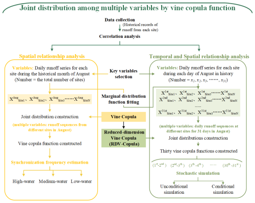
The framework of this study is shown in Fig. 1. This section focuses on constructing and applying multivariate joint distribution functions based on the vine copula function. It is divided into two cases: one considering only spatial relations and the other combining spatial and temporal relations. Utilizing the data characteristics, it describes how to build a vine copula function based on multiple variables and details the processes of synchronization frequency analysis and stochastic simulation with the constructed vine copula function. Additionally, it presents a new approach called the reduced-dimension vine copula (RDV-Copula).

Figure 1 Framework of the proposed methodology.

2.1 Joint distribution of multiple variables

Before identifying the dependence relationships among multiple variables, their correlations need to be analyzed and judged. Kendall's correlation coefficient, a nonparametric statistic, serves to measure the correlation degree between two variables, making it suitable for nonlinear relationships and categorical variables. In this study, vine copula functions are constructed to achieve a synchronization frequency and stochastic simulation of multiple streamflow sequences. To more accurately simulate the temporal and spatial relationships, the correlations among multi-site streamflow series are determined by calculating the Kendall correlation coefficients.

2.1.1 Marginal distribution function

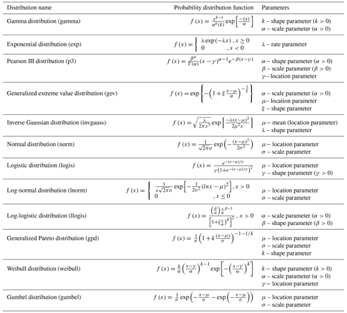
To build the dependence structure of hydrological variables using copulas, it is essential to determine the marginal distribution of each variable first. Given that the marginal distribution function for each characteristic variable is not predetermined and the skewness of their probability distributions varies (Zhong et al., 2021), it becomes crucial to consider multiple marginal distribution functions as candidates. In this study, a comprehensive comparison is conducted among 12 commonly utilized distributions (Tosunoğlu, 2018), including gamma distribution (gamma), exponential distribution (exp), Pearson III distribution (p3), generalized extreme value distribution (gev), inverse Gaussian distribution (invgauss), normal distribution (norm), logistic distribution (logis), log-normal distribution (lnorm), log-logistic distribution (llogis), generalized Pareto distribution (gpd), Weibull distribution (weibull), and Gumbel distribution (gumbel). According to the goodness-of-fit test and Akaike information criterion (AIC) minimum criterion, the optimal distribution functions are selected as the marginal functions of the characteristic variables. The specific details of different distributions, such as the probability distribution function and the respective parameters, are displayed in Appendix A.

2.1.2 Vine copula function theory

Copula functions, first introduced in 1959, represent a multivariate joint probability distribution function within the unit square [0, 1], featuring uniform marginal distributions. According to Sklar's theorem (Sklar, 1959), for a multivariate random variable $x_{\mathrm{1}},x_{\mathrm{2}},x_{\mathrm{3}},\mathrm{\dots },x_d$, there exist marginal distributions u₁=f₁(x₁), u₂=f₂(x₂), u₃=f₃(x₃), … , u_d=f_d(x_d) and joint distribution $f\left(x_{\mathrm{1}},x_{\mathrm{2}},x_{\mathrm{3}},\mathrm{\dots },x_d\right)$, and then there exists a copula function C_θ such that

$$\begin{array}{}\text{(1)}& \begin{array}{rl}& f\left(x_{\mathrm{1}},x_{\mathrm{2}},x_{\mathrm{3}},\mathrm{\dots },x_d\right)=C_{\mathit{\theta }}\left[f_{\mathrm{1}}\left(x_{\mathrm{1}}\right),f_{\mathrm{2}}\left(x_{\mathrm{2}}\right),\mathrm{\dots },f_d\left(x_d\right)\right]\\ & =C_{\mathit{\theta }}\left(u_{\mathrm{1}},u_{\mathrm{2}},\mathrm{\dots },u_d\right).\end{array}\end{array}$$

If f₁(x₁), f₂(x₂), … , f_d(x_d) are continuous functions, then C is unique. θ represents an explicit parameter of the function.

The multivariate conditional density function can be represented as follows:

$$\begin{array}{}\text{(2)}& f\left(x|\mathit{\nu }\right)=C_{\left.x{\mathit{\nu }}_j\right|{\mathit{\nu }}_{-j}}\left(F\left(\left.x\right|{\mathit{\nu }}_{-j}\right),F\left(\left.{\mathit{\nu }}_j\right|{\mathit{\nu }}_{-j}\right)\right)f\left(\left.x\right|{\mathit{\nu }}_{-j}\right),\end{array}$$

where ν_j denotes a component of the n-dimensional vector ν, while ν_−j denotes the (n−1)-dimensional vector with ν_j removed.

The term f(x | ν) in each conditional density function can be denoted as

$$\begin{array}{}\text{(3)}& F\left(x|\mathit{\nu }\right)={\displaystyle \frac{\partial C_{\left.x{\mathit{\nu }}_j\right|{\mathit{\nu }}_{-j}}\left(F\left(\left.x\right|{\mathit{\nu }}_{-j}\right),F\left(\left.{\mathit{\nu }}_j\right|{\mathit{\nu }}_{-j}\right)\right)}{F\left(\left.{\mathit{\nu }}_j\right|{\mathit{\nu }}_{-j}\right)}}.\end{array}$$

The copula function, essentially, acts as a transformation function that connects the joint distribution of multiple variables to the marginal distributions. There are a number of alternative copula families that can be selected for the construction of modeling dependence, such as the Gaussian copula, t copula, Clayton copula, Gumbel copula, and Frank copula. However, the construction of high-dimensional copula functions is often constrained by parameter limitations and is computationally demanding. Bedford and Cooke (2002) introduced a more advanced and flexible alternative method of constructing the dependence structure called vine copula. Also later called pair-copula construction by Aas et al. (2009a), vine copulas decompose the joint density function into a cascade of building blocks of the bivariate copulas. Assuming that there are d variables given to us, it is possible by this method to decompose the d-dimensional joint distribution into $d\left(d-\mathrm{1}\right)/\mathrm{2}$ pair-copula densities. In vine copula structure, the vine consists of a series of trees, nodes, and edges. The trees represent the layers. Each layer contains several nodes, and the connections between the nodes are called the edges. The nodes in the first tree represent the marginal distributions of each variable. Each edge represents a pair-copula joint distribution function of two adjacent nodes. The edges in each tree except the last tree are used as nodes in the next tree. There are two subsets of regular vines in common use: canonical vines (C-vine copulas) and drawable vines (D-vine copulas). Both types of vine copula have their own specific way of decomposing the density function.

In the C-vine copula structure, each tree features a central node that is connected to all other edges, as illustrated in Fig. 2a. The C-vine copula is suitable for structures with a key variable that has a significant correlation with the remaining other variables. In contrast, in the D-vine copula structure, each node is connected to no more than two edges, as depicted in Fig. 2b. The order of dependencies between variables can be determined by one after the other. The expressions for the n-dimensional joint probability density of C-vine and D-vine copulas are shown in Eqs. (4) and (5).

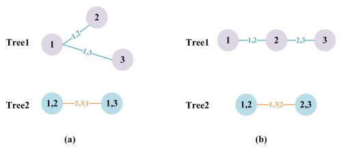
Figure 2 The vine structures for the given order of three variables in (a) the C-vine copula and (b) the D-vine copula.

$$\begin{array}{}\text{(4)}& {\displaystyle }\begin{array}{rl}f\left(x_{\mathrm{1}},\mathrm{\dots },x_d\right)& =\left[{\prod }_{j=\mathrm{1}}^{d-\mathrm{1}}{\prod }_{i=\mathrm{1}}^{d-j}{c}_{j,j+\mathrm{1}\left|\mathrm{1},\mathrm{\dots },j-\mathrm{1}\right.}\right]\\ & \cdot \left[{\prod }_{k=\mathrm{1}}^d{f}_k\left(x_k\right)\right]\left(\text{C-vine copula}\right),\end{array}\text{(5)}& {\displaystyle }\begin{array}{rl}f\left(x_{\mathrm{1}},\mathrm{\dots },x_d\right)& =\left[{\prod }_{j=\mathrm{1}}^{d-\mathrm{1}}{\prod }_{i=\mathrm{1}}^{d-j}{c}_{i,\left(i+j\right)\left|\left(i+\mathrm{1}\right),\mathrm{\dots },\left(i+j-\mathrm{1}\right)\right.}\right]\\ & \cdot \left[{\prod }_{k=\mathrm{1}}^d{f}_k\left(x_k\right)\right]\left(\text{D-vine copula}\right),\end{array}\end{array}$$

where c() refers to the bivariate copula with index i running over the edges for each tree and index j identifying the trees and f_k(x_k) denotes the marginal density.

2.2 Estimation of inflow synchronization frequency

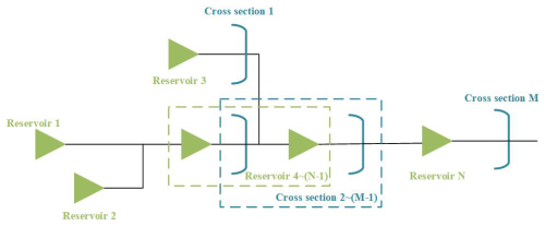
A distinct advantage of the copula method lies in its precision in analyzing inflow encounter probabilities and conditional probabilities. In this study, a synchronization event is defined as the simultaneous occurrence of inflows of similar magnitudes from multiple sites. We categorize the flow into three levels: high, medium, and low. The frequencies associated with high-water and low-water events are set to P_h=37.5 % and P_l=62.5 %. It is assumed that there is a generalized reservoir group scheduling system, as shown in Fig. 3. The system encompasses N reservoirs and M flood control cross sections.

Figure 3 Schematic diagram of the generalized system in the catchment.

We can generalize all reservoirs and cross sections to multiple sites within the watershed system. Each of these sites may be exposed to incoming flows when rainfall occurs. Let X_ph and X_pl be the amount of water corresponding to P_h and P_l, respectively. X_i>X_ph corresponds to high water (H), X_i<X_pl corresponds to low water (L), and $X_{\mathrm{pl}}<X_i<X_{\mathrm{ph}}$ corresponds to medium water (M), where X_i denotes the inflow of day i.

Let the inflows of the different sites be represented by $X^{\mathrm{1}},X^{\mathrm{2}},X^{\mathrm{3}},\mathrm{\dots },X^{N+M}$. $X_{\mathrm{ph}}^{\mathrm{1}},X_{\mathrm{ph}}^{\mathrm{2}},X_{\mathrm{ph}}^{\mathrm{3}},\mathrm{\dots },X_{\mathrm{ph}}^{N+M}$ represent the amount of inflow corresponding to the high water of these different sites, respectively. Meanwhile, $X_{\mathrm{pl}}^{\mathrm{1}},X_{\mathrm{pl}}^{\mathrm{2}},X_{\mathrm{pl}}^{\mathrm{3}},\mathrm{\dots },X_{\mathrm{pl}}^{N+M}$ represent the amount of inflow corresponding to the low water of these different sites, respectively. The marginal distribution functions are $u^{\mathrm{1}},u^{\mathrm{2}},u^{\mathrm{3}},\mathrm{\dots },u^{N+M}$, respectively. Specifically, $u_{\mathrm{ph}}^{\mathrm{1}},u_{\mathrm{ph}}^{\mathrm{2}},u_{\mathrm{ph}}^{\mathrm{3}},\mathrm{\dots },u_{\mathrm{ph}}^{N+M}$ denote the marginal distribution functions corresponding to the high-water inflow amount $X_{\mathrm{ph}}^{\mathrm{1}},X_{\mathrm{ph}}^{\mathrm{2}},X_{\mathrm{ph}}^{\mathrm{3}},\mathrm{\dots },X_{\mathrm{ph}}^{N+M}$, capturing the probabilistic behavior of the inflows during high-water conditions at each site. Similarly, $u_{\mathrm{pl}}^{\mathrm{1}},u_{\mathrm{pl}}^{\mathrm{2}},u_{\mathrm{pl}}^{\mathrm{3}}\mathrm{\dots },u_{\mathrm{pl}}^{N+M}$ represent the marginal distribution functions for the low-water inflow amount $X_{\mathrm{pl}}^{\mathrm{1}},X_{\mathrm{pl}}^{\mathrm{2}},X_{\mathrm{pl}}^{\mathrm{3}},\mathrm{\dots },X_{\mathrm{pl}}^{N+M}$, describing the inflow behavior during low-water conditions at these sites.

The number of possible inflow-state combinations increases with the number of sites, which are then directly tied to the three distinct states (high, medium, or low) identified for each site. For instance, with just two sites, there are nine unique combinations. The number of combinations expands to 27 for three sites, 81 for four sites, and 243 for five sites. The pattern continues similarly for additional sites. Take the combinations of four sites as an example; following the copula theory, $P\left(X^{\mathrm{1}}<x^{\mathrm{1}},X^{\mathrm{2}}<x^{\mathrm{2}}\right)=f\left(u^{\mathrm{1}},u^{\mathrm{2}}\right)=C\left(u^{\mathrm{1}},u^{\mathrm{2}}\right)$ and $P\left(X>x\right)=\mathrm{1}-P\left(X<x\right)$, the probability formulas of synchronization are derived as below.

1. The probability of synchronized high water is as follows:

   $$\begin{array}{}\text{(6)}& \begin{array}{rl}& P\left(X^{\mathrm{1}}>X_{\mathrm{ph}}^{\mathrm{1}},X^{\mathrm{2}}>X_{\mathrm{ph}}^{\mathrm{2}},X^{\mathrm{3}}>X_{\mathrm{ph}}^{\mathrm{3}},X^{\mathrm{4}}>X_{\mathrm{ph}}^{\mathrm{4}}\right)\\ & =\mathrm{1}-u_{\mathrm{ph}}^{\mathrm{1}}-u_{\mathrm{ph}}^{\mathrm{2}}-u_{\mathrm{ph}}^{\mathrm{3}}-u_{\mathrm{ph}}^{\mathrm{4}}+C\left(u_{\mathrm{ph}}^{\mathrm{1}},u_{\mathrm{ph}}^{\mathrm{2}}\right)\\ & +C\left(u_{\mathrm{ph}}^{\mathrm{1}},u_{\mathrm{ph}}^{\mathrm{3}}\right)+C\left(u_{\mathrm{ph}}^{\mathrm{1}},u_{\mathrm{ph}}^{\mathrm{4}}\right)+C\left(u_{\mathrm{ph}}^{\mathrm{2}},u_{\mathrm{ph}}^{\mathrm{3}}\right)\\ & +C\left(u_{\mathrm{ph}}^{\mathrm{2}},u_{\mathrm{ph}}^{\mathrm{4}}\right)+C\left(u_{\mathrm{ph}}^{\mathrm{3}},u_{\mathrm{ph}}^{\mathrm{4}}\right)-C\left(u_{\mathrm{ph}}^{\mathrm{1}},u_{\mathrm{ph}}^{\mathrm{2}},u_{\mathrm{ph}}^{\mathrm{3}}\right)\\ & -C\left(u_{\mathrm{ph}}^{\mathrm{1}},u_{\mathrm{ph}}^{\mathrm{2}},u_{\mathrm{ph}}^{\mathrm{4}}\right)-C\left(u_{\mathrm{ph}}^{\mathrm{1}},u_{\mathrm{ph}}^{\mathrm{3}},u_{\mathrm{ph}}^{\mathrm{4}}\right)\\ & -C\left(u_{\mathrm{ph}}^{\mathrm{2}},u_{\mathrm{ph}}^{\mathrm{3}},u_{\mathrm{ph}}^{\mathrm{4}}\right)+C\left(u_{\mathrm{ph}}^{\mathrm{1}},u_{\mathrm{ph}}^{\mathrm{2}},u_{\mathrm{ph}}^{\mathrm{3}},u_{\mathrm{ph}}^{\mathrm{4}}\right).\end{array}\end{array}$$

2. The probability of synchronized medium water is as follows:

   $$\begin{array}{}\text{(7)}& \begin{array}{rl}P& =(X_{\mathrm{pl}}^{\mathrm{1}}<X^{\mathrm{1}}<X_{\mathrm{ph}}^{\mathrm{1}},X_{\mathrm{pl}}^{\mathrm{2}}<X^{\mathrm{2}}<X_{\mathrm{ph}}^{\mathrm{2}},X_{\mathrm{pl}}^{\mathrm{3}}<X^{\mathrm{3}}<X_{\mathrm{ph}}^{\mathrm{3}},\\ & X_{\mathrm{pl}}^{\mathrm{4}}<X^{\mathrm{4}}<X_{\mathrm{ph}}^{\mathrm{4}})=C\left(u_{\mathrm{ph}}^{\mathrm{1}},u_{\mathrm{ph}}^{\mathrm{2}},u_{\mathrm{ph}}^{\mathrm{3}},u_{\mathrm{ph}}^{\mathrm{4}}\right)\\ & -C\left(u_{\mathrm{ph}}^{\mathrm{1}},u_{\mathrm{ph}}^{\mathrm{2}},u_{\mathrm{ph}}^{\mathrm{3}},u_{\mathrm{pl}}^{\mathrm{4}}\right)-C\left(u_{\mathrm{ph}}^{\mathrm{1}},u_{\mathrm{ph}}^{\mathrm{2}},u_{\mathrm{pl}}^{\mathrm{3}},u_{\mathrm{ph}}^{\mathrm{4}}\right)\\ & -C\left(u_{\mathrm{ph}}^{\mathrm{1}},u_{\mathrm{pl}}^{\mathrm{2}},u_{\mathrm{ph}}^{\mathrm{3}},u_{\mathrm{ph}}^{\mathrm{4}}\right)-C\left(u_{\mathrm{pl}}^{\mathrm{1}},u_{\mathrm{ph}}^{\mathrm{2}},u_{\mathrm{ph}}^{\mathrm{3}},u_{\mathrm{ph}}^{\mathrm{4}}\right)\\ & +C\left(u_{\mathrm{ph}}^{\mathrm{1}},u_{\mathrm{ph}}^{\mathrm{2}},u_{\mathrm{pl}}^{\mathrm{3}},u_{\mathrm{pl}}^{\mathrm{4}}\right)+C\left(u_{\mathrm{ph}}^{\mathrm{1}},u_{\mathrm{pl}}^{\mathrm{2}},u_{\mathrm{ph}}^{\mathrm{3}},u_{\mathrm{pl}}^{\mathrm{4}}\right)\\ & +C\left(u_{\mathrm{pl}}^{\mathrm{1}},u_{\mathrm{ph}}^{\mathrm{2}},u_{\mathrm{ph}}^{\mathrm{3}},u_{\mathrm{pl}}^{\mathrm{4}}\right)+C\left(u_{\mathrm{ph}}^{\mathrm{1}},u_{\mathrm{pl}}^{\mathrm{2}},u_{\mathrm{pl}}^{\mathrm{3}},u_{\mathrm{ph}}^{\mathrm{4}}\right)\\ & +C\left(u_{\mathrm{pl}}^{\mathrm{1}},u_{\mathrm{ph}}^{\mathrm{2}},u_{\mathrm{pl}}^{\mathrm{3}},u_{\mathrm{ph}}^{\mathrm{4}}\right)+C\left(u_{\mathrm{pl}}^{\mathrm{1}},u_{\mathrm{pl}}^{\mathrm{2}},u_{\mathrm{ph}}^{\mathrm{3}},u_{\mathrm{ph}}^{\mathrm{4}}\right)\\ & -C\left(u_{\mathrm{ph}}^{\mathrm{1}},u_{\mathrm{pl}}^{\mathrm{2}},u_{\mathrm{pl}}^{\mathrm{3}},u_{\mathrm{pl}}^{\mathrm{4}}\right)-C\left(u_{\mathrm{pl}}^{\mathrm{1}},u_{\mathrm{ph}}^{\mathrm{2}},u_{\mathrm{pl}}^{\mathrm{3}},u_{\mathrm{pl}}^{\mathrm{4}}\right)\\ & -C\left(u_{\mathrm{pl}}^{\mathrm{1}},u_{\mathrm{pl}}^{\mathrm{2}},u_{\mathrm{ph}}^{\mathrm{3}},u_{\mathrm{pl}}^{\mathrm{4}}\right)-C\left(u_{\mathrm{pl}}^{\mathrm{1}},u_{\mathrm{pl}}^{\mathrm{2}},u_{\mathrm{pl}}^{\mathrm{3}},u_{\mathrm{ph}}^{\mathrm{4}}\right)\\ & +C\left(u_{\mathrm{pl}}^{\mathrm{1}},u_{\mathrm{pl}}^{\mathrm{2}},u_{\mathrm{pl}}^{\mathrm{3}},u_{\mathrm{pl}}^{\mathrm{4}}\right).\end{array}\end{array}$$

3. The probability of synchronized low water is as follows:

   $$\begin{array}{}\text{(8)}& \begin{array}{rl}& P\left(X^{\mathrm{1}}<X_{\mathrm{pl}}^{\mathrm{1}},X^{\mathrm{2}}<X_{\mathrm{pl}}^{\mathrm{2}},X^{\mathrm{3}}<X_{\mathrm{pl}}^{\mathrm{3}},X^{\mathrm{4}}<X_{\mathrm{pl}}^{\mathrm{4}}\right)=\\ & C\left(u_{\mathrm{pl}}^{\mathrm{1}},u_{\mathrm{pl}}^{\mathrm{2}},u_{\mathrm{pl}}^{\mathrm{3}},u_{\mathrm{pl}}^{\mathrm{4}}\right).\end{array}\end{array}$$

2.3 Stochastic simulation based on RDV-Copula functions

2.3.1 Reduced-dimension vine copula construction approach (RDV-Copula) for multi-variate processes

To construct joint distribution functions for multiple variables that encapsulate both temporal and spatial relationships, it is essential to incorporate a comprehensive range of information to efficiently capture the interconnections among variables.

Using the flow at N points within a catchment as an example, the relationships among the flows are analyzed. Given that these points reside within the same geographical region, it is highly likely that they are spatially related and the strength of the relationship is negatively correlated with spatial distance. Additionally, each site exhibits temporal correlations, such as the relationship between today's flow and that of the previous day(s), although for simplicity, this analysis assumes relevance only between consecutive days' flows. Incorporating both temporal and spatial dimensions into the analysis implies that for N sites, there should ideally be N+N variables considered in constructing the copula function. As the number of sites grows, it simultaneously elevates the dimensionality of the copula, leading to increasingly complex structures. This complexity not only escalates computational efforts but also poses significant challenges in accurately fitting the model. To address this issue, our study introduces a novel methodology termed the reduced-dimension vine copula construction approach (RDV-Copula). This strategy aims to extract essential spatial–temporal information, thereby reducing the vine copula function's dimensionality to simplify the model structure.

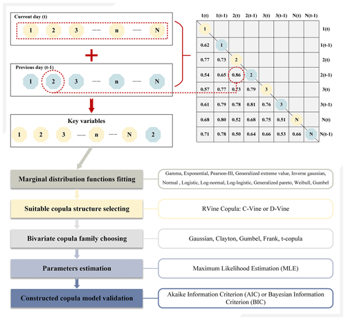
The primary goal of this approach is to pinpoint the crucial variables necessary for effectively and efficiently representing the spatial–temporal relationships among different sites. The process begins by identifying variables to capture spatial relationships under the assumption that the spatial relationships remain stable over short periods. Consequently, the current days' flows across all sites are selected as spatial variables, totaling N. Subsequently, the Kendall correlation coefficient between the current and previous day's flows is computed for each site, with the values ranked in descending order. The site with the highest Kendall coefficient is deemed the most temporally correlated, and its previous day's flow is also chosen as a key variable for the vine copula construction. Flows from the previous day at other sites are excluded from being key variables. Ultimately, this approach selects N+1 key variables, achieving an effective representation of spatial–temporal relationships while minimizing variable count. The schematic diagram of the process is shown in Fig. 4.

Figure 4 Schematic diagram of the RDV-Copula method.

After identifying the N+1 key variables, the marginal distribution function for each variable is determined, selecting the most appropriate distribution (e.g., normal, gamma) based on the statistical characteristics of each variable. Using these marginal distributions, a suitable copula structure is then selected, such as the C-vine or D-vine copula structure, depending on the nature of dependencies among the key variables. Next, for each pair of variables in the chosen vine structure, the most appropriate bivariate copula family (e.g., Gaussian, Clayton, Gumbel) is selected to accurately capture their dependencies. Subsequently, parameters for each selected pair copula are estimated sequentially using methods like maximum likelihood estimation (MLE). Finally, the constructed copula model is validated using statistical criteria such as the Akaike information criterion (AIC) or Bayesian information criterion (BIC).

2.3.2 Stochastic simulation

Simulation methods for multivariate stochastic processes are categorized into two main types: unconditional and conditional simulations, as delineated by Wu et al. (2015). The key difference between these two simulation methods lies in whether specific data points are known in advance, before generating the simulation. Figure 5a and b illustrate the unconditional simulation and the conditional simulation, respectively.

Unconditional simulation. This approach, illustrated in Fig. 5a, generates random samples based solely on the marginal probability distribution without incorporating any existing data constraints. The probability distribution is shown in the upper-left plot, and random samples are generated simultaneously, resulting in the scatterplot below. The generated samples, represented by blue points, illustrate the joint variability according to their predefined marginal distributions. Since no prior information is used, each data point is in an unknown state before the simulation.

Conditional simulation. In this scenario, illustrated in Fig. 5b, the simulation takes into account pre-existing data conditions. The marginal probability distribution is displayed in the top-center plot, while the known conditional data are shown in the upper-right scatterplot (in pink). These known data points act as a constraint for generating new random samples. The resulting scatterplot below (blue and pink points) demonstrates how the conditional samples are influenced by both the marginal distribution and the specified conditions of the known data. This method allows for a tailored simulation that incorporates pre-existing data insights.

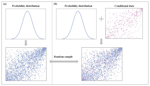
Figure 5 Schematic diagram for generating random simulation samples: (a) unconditional simulation and (b) conditional simulation.

Based on the presentation of each section in detail above, it can be generalized that stochastic simulation based on the RDV-Copula function needs to go through the following steps.

• Step 1. Collect as much historical data as possible.

• Step 2. Correlation analysis is conducted on the collected data by calculating Kendall's coefficient.

• Step 3. According to the method of filtering key variables proposed in Sect. 2.3.1, the representative key variables are extracted based on the correlation relationship among multiple variables.

• Step 4. Marginal distribution functions are fitted to the historical data series of the screened key variables.

• Step 5. Based on the proposed RDV-Copula approach, the joint distribution function of multi-site runoff sequences is constructed with consideration of spatial–temporal relationships.

• Step 6. The stochastic simulation sequences of runoff are generated by performing unconditional stochastic simulation and conditional stochastic simulation based on the constructed vine copula functions with different structures.

3 Case study

3.1 Study area and data description

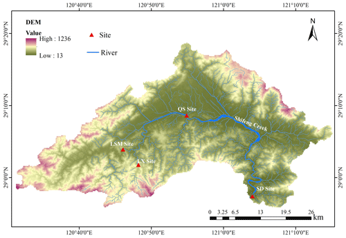
This study applies its methodology to a case study focusing on constructing spatial–temporal relationships within the Shifeng Creek area, located in the Jiao River catchment in eastern China. The Jiao River ranks as the third largest river in Zhejiang Province. As the primary tributary of the Jiao River basin and the principal watercourse in Tiantai County, Shifeng Creek plays a significant role. Rainfall distribution in the Shifeng Creek catchment is notably uneven throughout the year, with a substantial portion, approximately 70 % to 80 %, occurring from March to September. The remaining 20 % to 30 % of yearly rainfall is distributed over the other months. The period from July to September is particularly marked by intense storms and rainfall, largely influenced by the Pacific subtropical high-pressure system and the frequent occurrence of typhoons, and contributes about 35 % of the annual total precipitation, with the amount ranging from 400 to 600 mm.

The objective of this study is to delineate the spatial–temporal relationships of inflows within the catchment during August, a flood-prone month, to enhance flood pattern understanding and support effective flood management strategies. In the Shifeng Creek region, there are many important hydraulic structures and critical control cross sections. This study focuses on four major sites within the Shifeng Creek catchment: the Lishimen Reservoir (LSM) site; the Longxi Reservoir (LX) site, along with the Qianshan (QS) cross-section site; and the Shaduan (SD) cross-section site. These four sites were selected for their strategic importance within the Shifeng Creek catchment, covering the upper, middle, and lower reaches. The Lishimen (LSM) and Longxi (LX) reservoirs, both in the upper reaches, are vital for flood control, regulating inflows to reduce downstream flood risks. The Qianshan (QS) cross section, in the middle reaches, and the Shaduan (SD) cross section, in the lower reaches, serve as key flood control points. Analyzing flows at these sites enables better coordination of reservoir operations and prevents flood peak convergence, enhancing overall flood management. To achieve this, daily runoff data of August, covering a span from 2000 to 2020, were compiled. This dataset encompasses inflows for the LSM and LX reservoir sites as well as flow data for the QS and SD cross sections. The geographic positioning of Shifeng Creek is depicted in Fig. 6.

Figure 6 Map of the location of Shifeng Creek.

3.2 Numerical experiment setup

3.2.1 Synchronization frequency analysis based on spatial relationship

In this study, we employ the vine copula function to construct the joint distribution of runoff across four sites, aiming to analyze the synchronization frequency of floods in August, a month identified as having a high risk of flooding. The variables under consideration include the inflow from these four sites, denoted as LSM-Aug, LX-Aug, QS-Aug, and SD-Aug. Our initial step involves calculating the Kendall coefficients among these variables to assess their interdependencies. Following the methodology outlined in Sect. 2.1.1, we determine the marginal distribution functions of the four variables through a fitting test. Subsequently, based on the marginal distribution function of each variable, the joint distribution function of four variables is constructed. The parameters of the vine copula are estimated via the maximum likelihood method, with the Akaike information criterion (AIC) serving as the selection criterion to ensure optimal model fit. Upon passing the fitting test, we identify the most appropriate vine copula structure to accurately model the relationships among the variables.

With the four-dimensional vine copula function established, we proceed to calculate and analyze the synchronization frequency of inflows as described in Sect. 2.2. The inflows at the four sites are symbolized as LSM, LX, QS, and SD, with the high-water and low-water inflow amount represented as X_ph, Y_ph, Z_ph, and W_ph and X_pl, Y_pl, Z_pl, and W_pl, respectively. The marginal distribution functions are denoted as u, v, r, and s.

Considering the three potential states (high, medium, and low) at each site, a total of 81 possible inflow-state combinations are identified. For ease of presentation, H, M, and L are then used as abbreviations for high, medium, and low. Among the 81 combinations, the combinations [X-H, Y-H, Z-H, W-H], [X-M, Y-M, Z-M, W-M], and [X-L, Y-L, Z-L, W-L] are classified as synchronous high water, synchronous medium water, and synchronous low water, respectively, while the remainder are deemed asynchronous. The calculation equations can be provided in Appendix B.

3.2.2 Various vine copulas construction based on spatial–temporal relationships and stochastic simulation

To enhance the vine copula function's accuracy, it is imperative to integrate the temporal dimension into its construction. In this section, the vine copula functions are developed on a daily basis, encompassing a series of 31 copula models corresponding to each day of August, from the 1st to the 31st. Consequently, both Kendall correlation analysis and the fitting of marginal distribution functions must be independently conducted for the data spanning these 31 d. Following this preliminary analysis, 31 distinct relationship functions are constructed, each tailored to the specific type of vine copula identified for each day.

RDV-Copula function construction

Given that all four sites are situated within the Shifeng Creek watershed, their spatial interconnectivity is inherent and can be leveraged in constructing a vine copula function. Additionally, the results of the correlation analysis indicate that the correlation between the current day's runoff and the previous day's runoff is the highest. At the same time, the data from 2 d ago no longer have much influence on the current day's runoff data, so they can be excluded from the critical variable selection. Considering only the previous day's contribution in the time dimension can effectively represent the time correlation while avoiding an unnecessary dimension increase. This study integrates the inflows from the four sites over two consecutive days. The inflows for the current day are denoted as LSM, LX, QS, and SD, while those for the previous day are labeled LSM1, LX1, QS1, and SD1, respectively.

The methodology, as detailed in Sect. 2.3, is initiated by analyzing the current day's inflows at the four sites to establish their spatial relationships. The subsequent step involves identifying the site with the most significant correlation to its preceding day's inflow, which is then used as a variable to represent the temporal relationship on that day. For instance, analysis between 1 and 2 August reveals that the LSM site had the highest correlation with its prior day's flow compared to the other sites. Taking the construction of the copula function relationship between 1 and 2 August as an example, the analysis reveals that the LSM site has the highest correlation with its previous day's flow compared to the other three sites. As a result, a total of five key variables are determined for this relationship set, including LSM, LX, QS, SD, and LSM1, effectively encompassing both temporal and spatial correlations while streamlining the variable dimensions within the copula.

Due to the fundamental difference in structure between C-vine and D-vine copula, this study constructs five-dimensional RDV-Copula functions based on these two types, respectively, labeled as RDV-Cvine and RDV-Dvine. These two types of models should first be evaluated against each other on various indexes, including AIC, BIC, and Loglik, to ascertain the most suitable five-dimensional RDV-Copula structure. The RDV-Copula structure with better index values is then further compared with other copula functions to validate its efficacy.

Benchmark copula functions construction

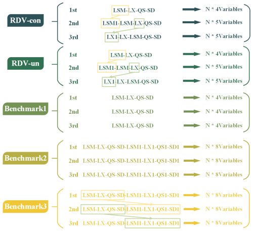
To validate the effectiveness of the RDV-Copula approach, this study compares it against a series of benchmark copula functions. These benchmarks are constructed by applying various combinations of multiple variables and stochastic simulation approaches to the existing data, resulting in vine copula models of differing dimensions. The specifics of these vine copula models are summarized as follows and illustrated in Fig. 7.

• Benchmark 1. This model focuses solely on spatial correlations, utilizing inflows at the four sites on the current day (LSM-LX-QS-SD) to create a four-dimensional vine copula. Simulations are conducted unconditionally.

• Benchmark 2. This model incorporates both spatial and temporal correlations, including inflows at the four sites for both the current and the previous day (LSM-LX-QS-SD-LSM1-LX1-QS1-SD1), resulting in an eight-dimensional vine copula. This model also employs unconditional simulation.

• Benchmark 3. Like Benchmark 2, this model considers both spatial and temporal correlations using the same set of key variables (LSM-LX-QS-SD-LSM1-LX1-QS1-SD1), thereby forming an eight-dimensional vine copula. However, it differs in its application of conditional simulation, assuming the previous day's runoff is a known condition to simulate the current day's flows.

To further detail the distinctions in stochastic simulation approaches, the RDV-Copula functions are bifurcated into two categories: RDV-un and RDV-con.

Both models account for spatial and temporal correlations by incorporating inflows at the four sites on the current day and the inflow at one site from the previous day (LSM-LX-QS-SD-X1), creating a five-dimensional vine copula. The variable X represents the site with the strongest temporal connection. RDV-un employs unconditional simulation, while RDV-con utilizes conditional simulation.

Figure 7 Five different vine copula models.

4 Results

4.1 Synchronization frequency analysis

Prior to performing a synchronization frequency analysis on multiple variables, it is imperative to conduct a correlation analysis to verify the presence of spatial correlations among them. Following the approach outlined in Sect. 2.1, this study begins with a correlation analysis of the daily runoff in August at the four selected sites, utilizing Kendall coefficients to quantify their interconnections. The results of this analysis, demonstrating the correlation among the four variables, are shown in Fig. 8a. The asterisk (*) on the ellipse means that the correlation passes the significance test of α=0.05. Subsequent to identifying correlation, the next step involves determining the marginal distributions for these variables. Figure 8b displays the results of this process, showcasing both the plots of the fitted marginal distributions for the four variables and the actual data distribution, thereby laying the groundwork for a comprehensive understanding of the data's distribution characteristics.

Figure 8 (a) Results of the correlation analysis for daily runoff at multiple sites. (b) Cumulative probability distribution of the preferred marginal distribution function.

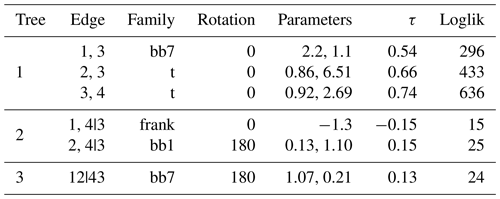
Figure 8 demonstrates that the correlations among the four study variables have all passed the significance test (p ≤0.05), with the QS and SD sites exhibiting the strongest correlations. This is closely followed by the spatial connections between the LX site and both QS and SD sites, with correlation coefficients of 0.67 and 0.65, respectively. The correlations involving the LSM site and the other three sites are relatively low, reflecting a reduction in spatial correlation with increasing distance. In terms of runoff distribution, the LSM site's runoff adheres to the Weibull distribution (weibull), while the runoff at the LX site fits the inverse Gaussian distribution (invgauss), and the runoffs at both QS and SD sites align with the log-normal distribution (lnorm). Building on the vine copula function methodology outlined in Sect. 2.1.2, we have developed a four-dimensional vine copula function using these variables. The function's structure, alongside the estimated parameters, is detailed in Table 1.

Table 1 Four-dimensional vine copula structure and parameters.

Upon the construction of four-dimensional vine copula function, the synchronization frequency analysis can be expanded. Using the approach detailed in Sect. 2.2, we obtained 81 encounter probabilities reflecting potential inflow scenarios at four sites: high-water, medium-water, and low-water scenarios. Figure 9a shows these 81 probabilities in detail. Figure 9b–g present aggregated views, focusing on nine combinations representing two of the four variables in each of their three states.

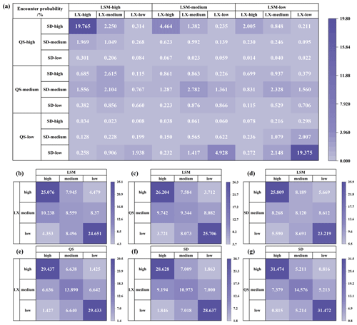
Figure 9 Encounter probabilities for multiple sites: (a) LSM-LX-QS-SD, (b) LSM-LX, (c) LSM-QS, (d) LSM-SD, (e) LX-QS, (f) LX-SD, and (g) QS-SD.

As observed in Fig. 9, the cumulative probability of synchronization across all four sites simultaneously stands at 41.92 %, encompassing three scenarios: (1) LSM-high, LX-high, QS-high, and SD-high; (2) LSM-medium, LX-medium, QS-medium, and SD-medium; and (3) LSM-low, LX-low, QS-low, and SD-low. Any two of these sites also demonstrate a very strong synchronization between them, with probabilities nearing 60 %. The obvious dark-colored blocks in the graph indicate the high probabilities of being in high-water or low-water states concurrently. Among these, the strongest synchronization occurs between the QS and SD sites, reaching a probability of 77.52 %. This is closely followed by the LX site's synchronization with both QS and SD sites at probabilities of 72.76 % and 68.24 %, respectively. While the LSM site's synchronization probabilities with the other sites are comparatively lower, they still exceed 50 %, with values of 58.29 % for the LX site, 61.25 % for the QS site, and 57.15 % for the SD site. This analysis underscores the clear spatial correlation among the four sites and highlights the critical importance of monitoring high-water synchronization. This is because such a case of simultaneous high water at multiple sites can easily induce flooding and pose a risk to the downstream. By analyzing the relationship of flow among multiple sites in advance and clarifying the probability of synchronization, it would be more conducive to the formulation of flood control and scheduling strategies to reduce the probability of flood encounters and ensure the safety of the downstream.

4.2 Construction of joint distributions of multi-site daily inflows

4.2.1 Correlation analysis

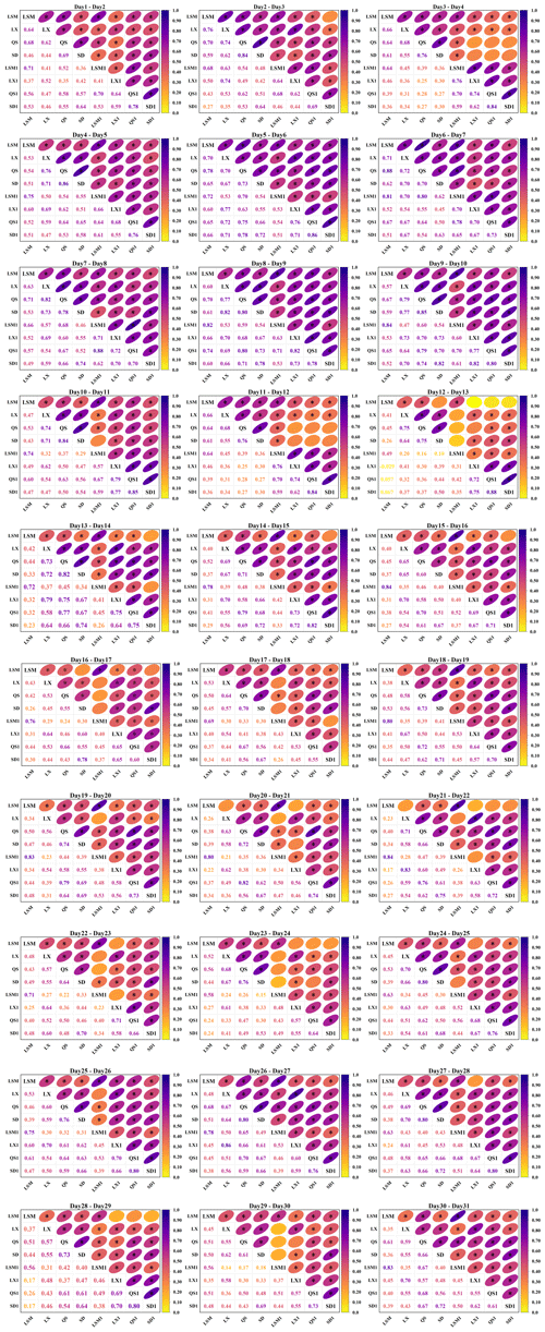
Correlation analysis serves as an efficient tool for quickly identifying and quantifying the correlations among multiple variables. Following the methodology outlined in Sect. 2.1, this study incorporates both temporal and spatial correlations in its analysis. To achieve this, historical runoff data from four key sites, along with the previous day's runoff data at each site, were used, resulting in a set of eight variables for the correlation analysis. The results of the analysis are presented in Fig. 10. Due to the large amount of information, only part of the correlation results is shown here. The complete set of results is available in Appendix C.

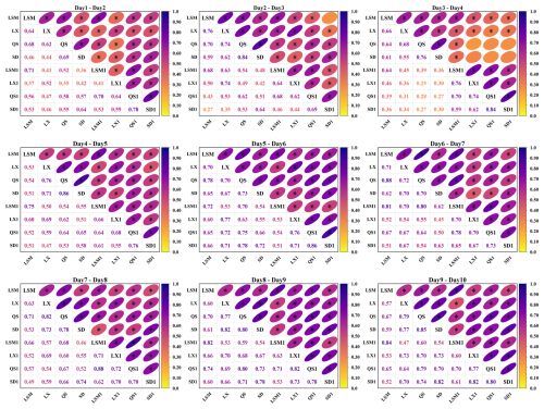
Figure 10 Partial results of the correlation analysis for daily runoff at multiple sites (LSM, LX, QS, and SD represent the runoff sequences of the current day, while LSM1, LX1, QS1, and SD1 represent the runoff sequences of the previous day).

Figure 10 illustrates the Kendall correlation coefficients between pairs of variables. The intensity of colors correlates with the strength of positive correlation, with darker shades signifying a correlation coefficient closer to 1. The asterisk (*) on the ellipse means that the correlation passes the significance test of α=0.05. This figure uncovers a marked positive correlation among the runoff series at the LSM, LX, QS, and SD sites, with approximately 93 % of these correlations meeting the significance threshold. This finding indicates that there is an obvious spatial correlation among the four locations. Notably, the QS and SD sites exhibit the strongest spatial correlation, with an average coefficient in August of 0.74, which is closely followed by the LX reservoir's correlation with the QS and SD sections at 0.67 and 0.63, respectively. In comparison, the LSM reservoir's runoff shows relatively lower correlations with the other sites, averaging 0.48 at the LX site, 0.55 at the QS site, and 0.45 at the SD site in August.

Upon analyzing the temporal correlation of runoff at each site for adjacent days within August (denoted as LSM-LSM1, LX-LX1, QS-QS1, and SD-SD1), it becomes evident that temporal correlations are significant and should not be overlooked. In early August in particular, these correlations register at a notably high level, suggesting more frequent flooding during this period. The LSM site demonstrates a standout temporal correlation, averaging 0.72 in August, indicative of a strong link between the current and previous day's runoff. The other sites display slightly lower, yet significant, temporal correlations: LX at 0.65, QS at 0.65, and SD at 0.67. When these temporal correlations are considered alongside the spatial ones, it is evident that LSM's temporal correlation surpasses its spatial correlation with other sites.

These correlation analysis results solidly confirm both spatial and temporal correlations among the four sites, laying a foundational basis for advancing with the construction of a copula structural model.

4.2.2 Fitting of marginal distribution of each runoff

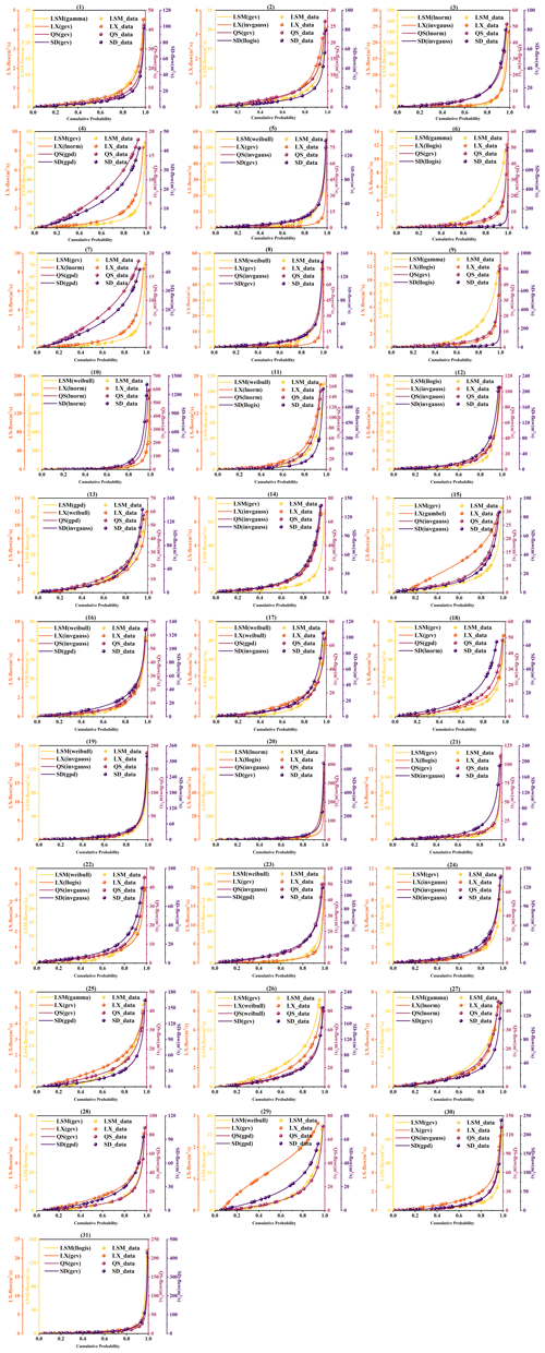
In this study, 12 distinct distribution functions were utilized to model the daily runoff at four sites throughout August. To assess the goodness of fit of these distributions, the Kolmogorov–Smirnov (K–S) test with a significance level of 0.05 was employed. Following a successful significance test, the Akaike information criterion (AIC) minimum method was applied to evaluate and determine the optimal marginal distribution for each dataset. Figure 11 shows the preferred marginal distribution functions for each variable over the 31 d of August. This figure contrasts the actual historical data points against the curves of the fitted functions, offering a visual representation of the fitting accuracy. The specific marginal distribution functions chosen for each variable, along with their parameters for each day, are comprehensively listed in Appendix D. Figure 11 notably illustrates how well these selected marginal distribution functions match the actual data for all four variables from 1 to 12 August. The chosen marginal distribution functions for the entire month are detailed in Fig. D1. Furthermore, the figure's legend explicitly details the types of fitting functions employed for each variable, providing a clear and comprehensive overview of the distributional characteristics.

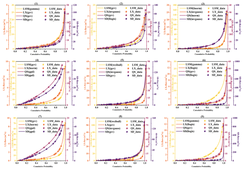
Figure 11 Cumulative probability distribution of the preferred marginal distribution function for runoff on each day throughout 1–9 August.

The distribution of the corresponding marginal distribution functions for the four variables over the 31 d in August is summarized in Fig. 12.

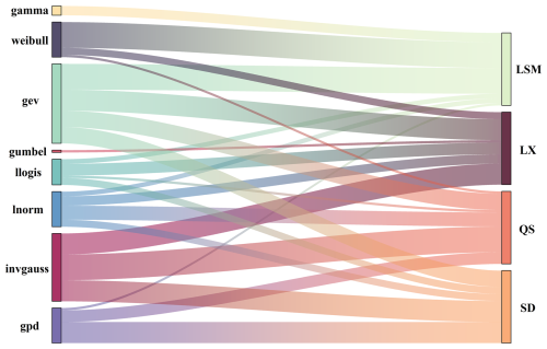
Figure 12 Distribution of the preferred marginal distribution function for the daily series of flows at the LSM, LX, QS, and SD sites in August.

Figure 12 shows that most streamflow series follow the gev distribution (27.52 %) and the invgauss distribution (23.39 %). Relatively few streamflow series follow the weibull, llogis, lnorm, and gpd distributions, and only a very small number follow the gamma and gumbel distributions. Additionally, 71 % of the runoff sequences at the LSM site follow the weibull and gev distributions, each accounting for 35.5 %. The runoff sequences at the LX site, the QS site, and the SD site predominantly follow the gev and invgauss distributions, accounting for 29.03 % and 29.03 % at the LX site, 22.58 % and 35.48 % at the QS site, and 22.58 % and 29.03 % at the SD site, respectively. Meanwhile, nearly 30 % of the runoff sequences at the SD site also follow the gpd distribution.

4.2.3 Construction of the RDV-Copula function

Following the identification of each variable's marginal distribution, the next step involves selecting the appropriate copula structures to construct the vine copula models among the multiple variables. Utilizing the RDV-Copula function construction approach described in the section “RDV-Copula function construction”, we identified the sites exhibiting the highest temporal correlation for each day in August based on our correlation analysis results. The variables chosen for each specific day are illustrated in Fig. 13.

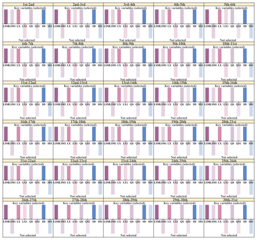
Figure 13 Key factors in the five-dimensional vine copula structure constructed on two adjacent days (LSM, LX, QS, and SD represent the runoff sequences of the current day, while LSM1, LX1, QS1, and SD1 represent the runoff sequences of the previous day).

Prior to selecting a specific copula function for modeling, it is essential to decide on the type of copula to be employed. Among the options, C-vine and D-vine structures stand out for their common use in various applications. In this study, we constructed both C-vine and D-vine copula structures for the set of multiple variables under consideration. To evaluate the efficacy of these structures, metrics such as the Akaike information criterion (AIC), Bayesian information criterion (BIC), and log-likelihood (Loglik) values were utilized and computed, with the results presented in Fig. 14. The AIC and BIC values reveal that for the majority of cases, the D-vine copula structures exhibit significantly lower values compared to those of the C-vine structures. Lower values in these criteria suggest a model's better performance and fit. Moreover, the comparison of log-likelihood values also showed that D-vine structures typically yielded lower values than their C-vine counterparts. Consequently, the D-vine copula structure was identified as more effective and suitable for modeling the intricate relationships among the variables in this study. Therefore, the RDV-Copula and other benchmark copula models were designed using the D-vine structure.

Figure 14 Comparison of the performance of RDV-Copula models for C-vine and D-vine (a) AIC, (b) BIC, and (c) log likelihood.

A large number of copula families was utilized to model the joint distributions, such as the Gaussian copula, Gumbel copula, t copula and so on. Following the guidance of AIC criteria, the most suitable pair copula for each connection within every tree was selected. After fitting the goodness of the copula functions, we employed the maximum likelihood method to estimate the parameters. As an illustrative example, the copula structure for 1–2 August is shown in Fig. 15. This figure reveals not only the best-fit copula family for each pair of adjacent nodes but also the estimated parameters. The nodes, labeled 1 through 5, represent LSM, LX, QS, SD, and X1, which indicates the site with the highest temporal correlation on that day, respectively. In this instance, X1 corresponds to LSM1. It is important to note that the specific choice of X1 might vary from day to day as further elaborated in Fig. 13. In Fig. 15, each pair of panels situated between nodes shows two aspects of the bi-dimensional copula function for those nodes. The first panel presents the joint probability plot, while the second illustrates the joint probability density plot.

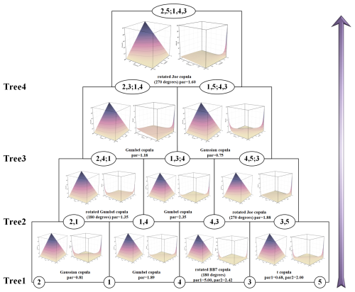
Figure 15 Structure of the five-dimensional D-vine copula model for 1–2 August (nodes 1–5 represent LSM, LX, QS, SD, and LSM1; the plots between each two nodes are schematic plots of the corresponding copula function, with the joint probability plot on the left and joint probability density plot on the right).

4.3 Stochastic simulation results of runoff from multiple sites

To validate the models and facilitate a comparative analysis of different vine copula functions, the following work was carried out. Initially, the constructed copula structure and the results from parameter estimation were incorporated into a simulation process, generating 20 000 sets of random runoff scenarios for each day in August. Considering August's susceptibility to flooding and the typical continuity of rainfall events, it is highly likely that runoff on consecutive days is temporally correlated. Therefore, comparing only the mean and standard deviation of runoff simulated for individual days might not fully capture the model's simulation efficacy. In this context, the study calculated the mean and standard deviation for the current day by considering the simulated flows of both the preceding and the following day. Ultimately, after the exclusion of outliers from the 20 000 sets of simulated runoff scenarios, the average of the mean and standard deviation calculated from these three days' simulated flows will be used as the mean and standard deviation for the current day. The runoff simulation results for the four locations (LSM, LX, QS, and SD) are presented in Figs. 16, 17, 18, and 19, respectively. Notably, in each figure, panel (a) displays the mean values and standard deviations from the simulation results for the five copula structures, allowing these results to be compared against historical observations for a nuanced evaluation of the simulation's performance. Panels (b), (c), (d), (e), and (f) represent the simulation results for five different sets of copula structures (RDV-con, RDV-un, Benchmark1, Benchmark2, and Benchmark3), respectively. The solid line in the figure is the mean of the simulation results, and the shaded area represents the uncertainty (±1 standard deviation) of the simulation.

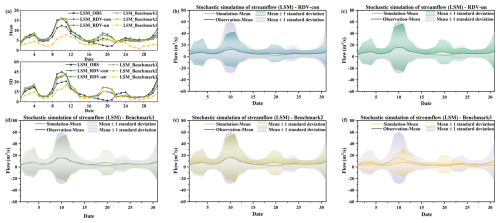
Figure 16 Comparison of the actual observed series with simulation results of four copula structures at the LSM site. (a) Comparison of daily runoff mean values and standard deviation. (b) Simulation results of RDV-con. (c) Simulation results of RDV-un. (d) Simulation results of Benchmark1. (e) Simulation results of Benchmark2. (f) Simulation results of Benchmark3.

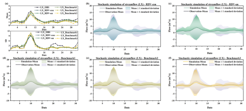
Figure 17 Comparison of the actual observed series with simulation results of four copula structures at the LX site (a) Comparison of daily runoff mean values and standard deviation. (b) Simulation results of RDV-con. (c) Simulation results of RDV-un. (d) Simulation results of Benchmark1. (e) Simulation results of Benchmark2. (f) Simulation results of Benchmark3.

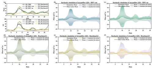
Figure 18 Comparison of the actual observed series with simulation results of four copula structures at the QS site (a) Comparison of daily runoff mean values and standard deviation. (b) Simulation results of RDV-con. (c) Simulation results of RDV-un. (d) Simulation results of Benchmark1. (e) Simulation results of Benchmark2. (f) Simulation results of Benchmark3.

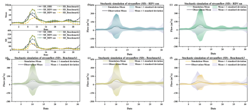
Figure 19 Comparison of the actual observed series with simulation results of four copula structures at the SD site (a) Comparison of daily runoff mean values and standard deviation. (b) Simulation results of RDV-con. (c) Simulation results of RDV-un. (d) Simulation results of Benchmark1. (e) Simulation results of Benchmark2. (f) Simulation results of Benchmark3.

From four figures, it is evident that the simulation results of RDV-Copula, Benchmark1, and Benchmark2 are comparatively more accurate. The mean values and standard deviations from these simulations closely match the actual observed runoff, particularly for simulations involving smaller flow magnitudes, where the accuracy aligns more precisely with the actual values. Although the RDV-Copula results are consistent with the benchmark models, they do not exhibit a marked advantage for smaller flows. However, in scenarios involving larger flows, such as those at the SD site, RDV-Copula models outperform other models, highlighting their superiority in capturing the characteristics of larger inflow events. This analysis suggests that for smaller flows, models focusing solely on spatial relationships suffice to capture the critical interrelationships among variables. In contrast, for larger flows, neglecting the influence of temporal correlations can lead to substantial inaccuracies in the simulation results, suggesting that larger flows are more significantly influenced by adjacent days' flows. Comparing the four figures, we can also find that the simulation results at the LX location consistently exhibit high accuracy, with the simulation results basically covering the actual observations. This suggests that the constructed copula models can easily extract the historical correlations and simulate them, particularly in smaller flow magnitudes.

However, the Benchmark3 model's performance is notably less effective among the five models. This suboptimal performance can be attributed to two main factors. Firstly, the complexity of the eight-dimensional copula function, which involves a diverse combination of trees, nodes, and various types of parameters, poses significant challenges in accurately extracting the relationship characteristics among the four sites. Secondly, the conditional simulation approach of Benchmark3, which relies on the previous day's flow at the four sites as a known condition for simulation, is highly susceptible to the accuracy of these initial conditions. If the simulation results for the previous day contain significant errors, these inaccuracies are likely to propagate through the simulation, leading to compounded errors in all results. Another noteworthy point is that the simulation results on 10, 20, and 31 August are not quite consistent with historical conditions. This is because the runoff on these three days has been at a low level for most of the time over a number of years in history. It is therefore a rather exceptional phenomenon that a major flood event occurred on these particular dates in just 1 year. Specifically, the data recorded on these dates (10 August 2009, 31 August 2011, and 20 August 2014) indicate unusually high runoff, which significantly exceeds their respective historical averages. Such an occurrence presents a challenge for the simulations as it requires accurately capturing and replicating these atypically high flow values within the model.

Comparing the two types of simulations of RDV-Copula, it can be found that the performances of the simulation results of RDV-un and RDV-con are at a similar level for LSM and LX sites. However, in the simulation of QS and SD sites, RDV-con shows an obvious superiority compared to RDV-un. This illustrates the better generalization of conditional simulation for such complex structure with spatial–temporal relationships. In contrast to the unconditional simulation, RDV-con can better utilize the temporal correlation to improve the accuracy of the simulation. Meanwhile, since it is different from the conditional simulation of the eight-dimensional vine copula (Benchmark2), RDV-con successfully reduces the cumulative error caused by the excessive dimensionality.

In summary, for the relational construction and stochastic simulation of flows across varying magnitudes, RDV-Copula and Benchmark2 emerge as more suitable, particularly when considering the influences of both temporal and spatial correlations. However, the use of an eight-dimensional copula function in Benchmark2 introduces significant computational demands and adds complexity to the problem. RDV-Copula is favored for its effective integration of temporal and spatial correlations along with the simplification of the copula structure, thereby streamlining the problem-solving process and enhancing computational efficiency.

5 Discussion

For variables with interdependencies, the copula function, increasingly popular in contemporary studies, extracts spatial–temporal relationships from their marginal distributions. Vine copulas are notably effective in modeling complex dependencies among variables as they offer substantial flexibility. This capability is exemplified in the work of Pereira and Veiga (2018), who developed a multivariate conditional model using D-vine copulas for simulating periodic streamflow scenarios, emphasizing the structured arrangement of variables to capture monthly flow dependencies. This and numerous other studies (Nazeri Tahroudi et al., 2022; Wang et al., 2018, 2019; Wang and Shen, 2023b) underscored the effectiveness of vine copulas in capturing dependencies among variables with differing marginal distributions.

The synchronous probability analysis of multi-site runoff shows that the vine copula model can be used to provide a good fit to the dependencies among variables obeying different marginal distributions. Similar conclusions have been obtained in other studies (Qian et al., 2022; Ren et al., 2020; Wei et al., 2023). In the study of Xu et al. (2022b), the multivariate Copula model was implemented to evaluate the synchronous–asynchronous characteristics for hydrological probabilities for multiple water sources. The simultaneous probabilistic analysis of multi-site runoff provides an understanding of the flood characteristics of the catchment leading to better flood control and prevention.

For high-dimensional variable dependency analysis, the structure of the vine copula is extremely complicated to construct. Depending on the number of hydrometric stations, Wang and Shen (2023b) established seven-dimensional regular vine (R-vine) copula models to depict the complex and diverse dependencies. To tackle the problem above, in their study, the corresponding vine structure was specified by the vine structure array that can reflect the sequence of tributaries flowing into the main stream and the spatial locations of different hydrometric stations. The performance of the ultimate simulation results was favorable, but it did not incorporate the temporal connection of the variables for each hydrometric station. If considered, it would lead to an exponential increase in the dimensionality of the variable. The RDV-Copula method proposed in this study aims to minimize the dimensionality of the copula model while extracting the effective information of spatial–temporal relationships. The evaluation criterion of high-performance stochastic simulation is that the simulated series can preserve the statistical characteristics of the observed records (Hao and Singh, 2013). As shown in Figs. 16–19, different vine copula structures have a large impact on the results of stochastic simulations. The simulation results of the four-dimensional and five-dimensional vine copula models are relatively closer to the actual historical values. Although the eight-dimensional vine copula model considers both temporal and spatial correlations, its complexity reduces simulation efficiency due to the large number of variables. This illustrates that when performing multi-site runoff simulations, it is not better for the vine copula function to consider as many variables as possible. Compared to the four-dimensional copula structure that only considers spatial relations, the five-dimensional copula structure can better fit the characteristics of high flows, which is especially evident in the simulation results of QS and SD points. This is due to the fact that high flows in flood season mostly originate from continuous heavy rainfall, which implies that the temporal connection is not negligible for capturing the flow characteristics.

Consequently, the approach introduced in this study effectively integrates all pertinent information for multi-site runoff simulations while reducing the complexity of the vine copula function. This methodology strikes a critical balance between detailed representation and practicality in model complexity, enhancing the applicability of the simulations.

6 Conclusions

This study introduced an innovative approach designed to capture the spatial–temporal relationships across multiple sites while simplifying the computational complexity inherent in vine copula functions. By computing Kendall correlation coefficients, we assessed the interconnections among various sites. Utilizing the approach proposed, we pinpointed the key variables for the construction of the vine copula model, fitted the marginal distribution functions for multiple variables, and constructed the RDV-Copula functions considering the spatial–temporal relationships. Subsequent to this, a synchronization frequency analysis based on the copula model was executed to delve deeper into the characteristics of the watershed. To gauge the efficacy of this method, three benchmark vine copula models, each predicated on different dimensions and variable relationships, were constructed. Stochastic simulations were then employed to generate arrays of daily inflow sequences over a typical flood month, with both conditional and unconditional simulation methods being critically compared. Key findings are summarized below.

• The results of our study demonstrated that within the Shifeng Creek watershed, the synchronization probability among the four sites reaches up to 41.92 %, with the average synchronization probability between any two sites hitting 65.87 %. This strong spatial connectivity indicates a potential for heavy-rainfall events to exacerbate flooding risks downstream.

• This study revealed that increasing model dimensions does not inherently improve simulation outcomes. The high-dimensional copula function, while it can capture more information on the variables, also makes the structure more complicated. The RDV-Copula method not only ensures comprehensive data integration but also diminishes the complexity and dimensionality of the vine copula function, showcasing an optimal balance between information accuracy and model simplicity.

• Conditional simulation is a double-edged sword. In comparison to unconditional simulation, for temporally correlated runoff sequences, conditional simulation can better follow the properties of prior conditions. However, with an increase in the copula's dimensionality, relying on previously simulated runoff as a basis for current-day predictions can accumulate errors, reducing the overall simulation accuracy.

In summary, our proposed approach can effectively consolidate relevant spatial–temporal information for multi-site runoff simulations, striking a critical balance between detailed representation and practical model complexity. This methodology enhances the applicability of vine copula models for analyzing and managing flood risks. The results obtained using this method can provide valuable decision support for flood control and scheduling, effectively mitigating flood risk.

Appendix A

Table A1 Common hydrological distribution functions.

Appendix B

The probability formulas for the 81 combinations are presented as follows.

1. The probability of type [X-H, Y-H, Z-H, W-H] is as follows:

   $P(X>X_{\mathrm{ph}},Y>Y_{\mathrm{ph}},Z>Z_{\mathrm{ph}},W>W_{\mathrm{ph}})=\mathrm{1}-u_{\mathrm{ph}}-v_{\mathrm{ph}}-r_{\mathrm{ph}}-s_{\mathrm{ph}}+C(u_{\mathrm{ph}},v_{\mathrm{ph}})+C(u_{\mathrm{ph}},r_{\mathrm{ph}})+C(u_{\mathrm{ph}},s_{\mathrm{ph}})+C(v_{\mathrm{ph}},r_{\mathrm{ph}})+C(v_{\mathrm{ph}},s_{\mathrm{ph}})+C(r_{\mathrm{ph}},s_{\mathrm{ph}})-C(u_{\mathrm{ph}},v_{\mathrm{ph}},r_{\mathrm{ph}})-C(u_{\mathrm{ph}},v_{\mathrm{ph}},s_{\mathrm{ph}})-C(u_{\mathrm{ph}},r_{\mathrm{ph}},s_{\mathrm{ph}})-C(v_{\mathrm{ph}},r_{\mathrm{ph}},s_{\mathrm{ph}})+C(u_{\mathrm{ph}},v_{\mathrm{ph}},r_{\mathrm{ph}},s_{\mathrm{ph}})$.

2. The probability of type [X-M, Y-M, Z-M, W-M] is as follows:

   $P=(X_{\mathrm{pl}}<X<X_{\mathrm{ph}},Y_{\mathrm{pl}}<Y<Y_{\mathrm{ph}},Z_{\mathrm{pl}}<Z<Z_{\mathrm{ph}},W_{\mathrm{pl}}<W<W_{\mathrm{ph}})=C(u_{\mathrm{ph}},v_{\mathrm{ph}},r_{\mathrm{ph}},s_{\mathrm{ph}})-C(u_{\mathrm{ph}},v_{\mathrm{ph}},r_{\mathrm{ph}},s_{\mathrm{pl}})-C(u_{\mathrm{ph}},v_{\mathrm{ph}},r_{\mathrm{pl}},s_{\mathrm{ph}})-C(u_{\mathrm{ph}},v_{\mathrm{pl}},r_{\mathrm{ph}},s_{\mathrm{ph}})-C(u_{\mathrm{pl}},v_{\mathrm{ph}},r_{\mathrm{ph}},s_{\mathrm{ph}})+C(u_{\mathrm{ph}},v_{\mathrm{ph}},r_{\mathrm{pl}},s_{\mathrm{pl}})+C(u_{\mathrm{ph}},v_{\mathrm{pl}},r_{\mathrm{ph}},s_{\mathrm{pl}})+C(u_{\mathrm{pl}},v_{\mathrm{ph}},r_{\mathrm{ph}},s_{\mathrm{pl}})+C(u_{\mathrm{ph}},v_{\mathrm{pl}},r_{\mathrm{pl}},s_{\mathrm{ph}})+C(u_{\mathrm{pl}},v_{\mathrm{ph}},r_{\mathrm{pl}},s_{\mathrm{ph}})+C(u_{\mathrm{pl}},v_{\mathrm{pl}},r_{\mathrm{ph}},s_{\mathrm{ph}})-C(u_{\mathrm{ph}},v_{\mathrm{pl}},r_{\mathrm{pl}},s_{\mathrm{pl}})-C(u_{\mathrm{pl}},v_{\mathrm{ph}},r_{\mathrm{pl}},s_{\mathrm{pl}})-C(u_{\mathrm{pl}},v_{\mathrm{pl}},r_{\mathrm{ph}},s_{\mathrm{pl}})-C(u_{\mathrm{pl}},v_{\mathrm{pl}},r_{\mathrm{pl}},s_{\mathrm{ph}})+C(u_{\mathrm{pl}},v_{\mathrm{pl}},r_{\mathrm{pl}},s_{\mathrm{pl}})$.

3. The probability of type [X-L, Y-L, Z-L, W-L] is as follows:

   $P(X<X_{\mathrm{pl}},Y<Y_{\mathrm{pl}},Z<Z_{\mathrm{pl}},W<W_{\mathrm{pl}})=C(u_{\mathrm{pl}},v_{\mathrm{pl}},r_{\mathrm{pl}},s_{\mathrm{pl}})$.

4. The probability of type [X-L, Y-H, Z-H, W-H] is as follows:

   $P(X<X_{\mathrm{pl}},Y>Y_{\mathrm{ph}},Z>Z_{\mathrm{ph}},W>W_{\mathrm{ph}})=u_{\mathrm{pl}}-C(u_{\mathrm{pl}},v_{\mathrm{ph}})-C(u_{\mathrm{pl}},r_{\mathrm{ph}})-C(u_{\mathrm{pl}},s_{\mathrm{ph}})+C(u_{\mathrm{pl}},v_{\mathrm{ph}},r_{\mathrm{ph}})+C(u_{\mathrm{pl}},v_{\mathrm{ph}},s_{\mathrm{ph}})+C(u_{\mathrm{pl}},r_{\mathrm{ph}},s_{\mathrm{ph}})-C(u_{\mathrm{pl}},v_{\mathrm{ph}},r_{\mathrm{ph}},s_{\mathrm{ph}})$.

5. The probability of type [X-H, Y-L, Z-H, W-H] is as follows:

   $P(X>X_{\mathrm{ph}},Y<Y_{\mathrm{pl}},Z>Z_{\mathrm{ph}},W>W_{\mathrm{ph}})=v_{\mathrm{pl}}-C(u_{\mathrm{ph}},v_{\mathrm{pl}})-C(v_{\mathrm{pl}},r_{\mathrm{ph}})-C(v_{\mathrm{pl}},s_{\mathrm{ph}})+C(u_{\mathrm{ph}},v_{\mathrm{pl}},r_{\mathrm{ph}})+C(u_{\mathrm{ph}},v_{\mathrm{pl}},s_{\mathrm{ph}})+C(v_{\mathrm{pl}},r_{\mathrm{ph}},s_{\mathrm{ph}})-C(u_{\mathrm{ph}},v_{\mathrm{pl}},r_{\mathrm{ph}},s_{\mathrm{ph}})$.

6. The probability of type [X-H, Y-H, Z-L, W-H] is as follows:

   $P(X>X_{\mathrm{ph}},Y>Y_{\mathrm{ph}},Z<Z_{\mathrm{pl}},W>W_{\mathrm{ph}})=r_{\mathrm{pl}}-C(u_{\mathrm{ph}},r_{\mathrm{pl}})-C(v_{\mathrm{ph}},r_{\mathrm{pl}})-C(r_{\mathrm{pl}},s_{\mathrm{ph}})+C(u_{\mathrm{ph}},v_{\mathrm{ph}},r_{\mathrm{pl}})+C(u_{\mathrm{ph}},r_{\mathrm{pl}},s_{\mathrm{ph}})+C(v_{\mathrm{ph}},r_{\mathrm{pl}},s_{\mathrm{ph}})-C(u_{\mathrm{ph}},v_{\mathrm{ph}},r_{\mathrm{pl}},s_{\mathrm{ph}})$.

7. The probability of type [X-H, Y-H, Z-H, W-L] is as follows:

   $P(X>X_{\mathrm{ph}},Y>Y_{\mathrm{ph}},Z>Z_{\mathrm{ph}},W<W_{\mathrm{pl}})=s_{\mathrm{pl}}-C(u_{\mathrm{ph}},s_{\mathrm{pl}})-C(v_{\mathrm{ph}},s_{\mathrm{pl}})-C(r_{\mathrm{ph}},s_{\mathrm{pl}})+C(u_{\mathrm{ph}},v_{\mathrm{ph}},s_{\mathrm{pl}})+C(u_{\mathrm{ph}},r_{\mathrm{ph}},s_{\mathrm{pl}})+C(v_{\mathrm{ph}},r_{\mathrm{ph}},s_{\mathrm{pl}})-C(u_{\mathrm{ph}},v_{\mathrm{ph}},r_{\mathrm{ph}},s_{\mathrm{pl}}).$

8. The probability of type [X-M, Y-H, Z-H, W-H] is as follows:

   $P(X_{\mathrm{pl}}<X<X_{\mathrm{ph}},Y>Y_{\mathrm{ph}},Z>Z_{\mathrm{ph}},W>W_{\mathrm{ph}})=u_{\mathrm{ph}}-u_{\mathrm{pl}}-C(u_{\mathrm{ph}},v_{\mathrm{ph}})-C(u_{\mathrm{ph}},r_{\mathrm{ph}})-C(u_{\mathrm{ph}},s_{\mathrm{ph}})+C(u_{\mathrm{pl}},v_{\mathrm{ph}})+C(u_{\mathrm{pl}},r_{\mathrm{ph}})+C(u_{\mathrm{pl}},s_{\mathrm{ph}})+C(u_{\mathrm{ph}},v_{\mathrm{ph}},r_{\mathrm{ph}})+C(u_{\mathrm{ph}},v_{\mathrm{ph}},s_{\mathrm{ph}})+C(u_{\mathrm{ph}},r_{\mathrm{ph}},s_{\mathrm{ph}})-C(u_{\mathrm{pl}},v_{\mathrm{ph}},r_{\mathrm{ph}})-C(u_{\mathrm{pl}},v_{\mathrm{ph}},s_{\mathrm{ph}})-C(u_{\mathrm{pl}},r_{\mathrm{ph}},s_{\mathrm{ph}})-C(u_{\mathrm{ph}},v_{\mathrm{ph}},r_{\mathrm{ph}},s_{\mathrm{ph}})+C(u_{\mathrm{pl}},v_{\mathrm{ph}},r_{\mathrm{ph}},s_{\mathrm{ph}})$.

9. The probability of type [X-H, Y-M, Z-H, W-H] is as follows:

   $P(X>X_{\mathrm{ph}},Y_{\mathrm{pl}}<Y<Y_{\mathrm{ph}},Z>Z_{\mathrm{ph}},W>W_{\mathrm{ph}})=v_{\mathrm{ph}}-v_{\mathrm{pl}}-C(u_{\mathrm{ph}},v_{\mathrm{ph}})-C(v_{\mathrm{ph}},r_{\mathrm{ph}})-C(v_{\mathrm{ph}},s_{\mathrm{ph}})+C(u_{\mathrm{ph}},v_{\mathrm{pl}})+C(v_{\mathrm{pl}},r_{\mathrm{ph}})+C(v_{\mathrm{pl}},s_{\mathrm{ph}})+C(u_{\mathrm{ph}},v_{\mathrm{ph}},r_{\mathrm{ph}})+C(u_{\mathrm{ph}},v_{\mathrm{ph}},s_{\mathrm{ph}})+C(v_{\mathrm{ph}},r_{\mathrm{ph}},s_{\mathrm{ph}})-C(u_{\mathrm{ph}},v_{\mathrm{pl}},r_{\mathrm{ph}})-C(u_{\mathrm{ph}},v_{\mathrm{pl}},s_{\mathrm{ph}})-C(v_{\mathrm{pl}},r_{\mathrm{ph}},s_{\mathrm{ph}})-C(u_{\mathrm{ph}},v_{\mathrm{ph}},r_{\mathrm{ph}},s_{\mathrm{ph}})+C(u_{\mathrm{ph}},v_{\mathrm{pl}},r_{\mathrm{ph}},s_{\mathrm{ph}})$.

10. The probability of type [X-H, Y-H, Z-M, W-H] is as follows:

    $P(X>X_{\mathrm{ph}},Y>Y_{\mathrm{ph}},Z_{\mathrm{pl}}<Z<Z_{\mathrm{ph}},W>W_{\mathrm{ph}})=r_{\mathrm{ph}}-r_{\mathrm{pl}}-C(u_{\mathrm{ph}},r_{\mathrm{ph}})-C(v_{\mathrm{ph}},r_{\mathrm{ph}})-C(r_{\mathrm{ph}},s_{\mathrm{ph}})+C(u_{\mathrm{ph}},r_{\mathrm{pl}})+C(v_{\mathrm{ph}},r_{\mathrm{pl}})+C(r_{\mathrm{pl}},s_{\mathrm{ph}})+C(u_{\mathrm{ph}},v_{\mathrm{ph}},r_{\mathrm{ph}})+C(u_{\mathrm{ph}},r_{\mathrm{ph}},s_{\mathrm{ph}})+C(v_{\mathrm{ph}},r_{\mathrm{ph}},s_{\mathrm{ph}})-C(u_{\mathrm{ph}},v_{\mathrm{ph}},r_{\mathrm{pl}})-C(u_{\mathrm{ph}},r_{\mathrm{pl}},s_{\mathrm{ph}})-C(v_{\mathrm{ph}},r_{\mathrm{pl}},s_{\mathrm{ph}})-C(u_{\mathrm{ph}},v_{\mathrm{ph}},r_{\mathrm{ph}},s_{\mathrm{ph}})+C(u_{\mathrm{ph}},v_{\mathrm{ph}},r_{\mathrm{pl}},s_{\mathrm{ph}})$.

11. The probability of type [X-H, Y-H, Z-H, W-M] is as follows:

    $P(X>X_{\mathrm{ph}},Y>Y_{\mathrm{ph}},Z>Z_{\mathrm{ph}},W_{\mathrm{pl}}<W<W_{\mathrm{ph}})=s_{\mathrm{ph}}-s_{\mathrm{pl}}-C(u_{\mathrm{ph}},s_{\mathrm{ph}})-C(v_{\mathrm{ph}},s_{\mathrm{ph}})-C(r_{\mathrm{ph}},s_{\mathrm{ph}})+C(u_{\mathrm{ph}},s_{\mathrm{pl}})+C(v_{\mathrm{ph}},s_{\mathrm{pl}})+C(r_{\mathrm{ph}},s_{\mathrm{pl}})+C(u_{\mathrm{ph}},v_{\mathrm{ph}},s_{\mathrm{ph}})+C(u_{\mathrm{ph}},r_{\mathrm{ph}},s_{\mathrm{ph}})+C(v_{\mathrm{ph}},r_{\mathrm{ph}},s_{\mathrm{ph}})-C(u_{\mathrm{ph}},v_{\mathrm{ph}},s_{\mathrm{pl}})-C(u_{\mathrm{ph}},r_{\mathrm{ph}},s_{\mathrm{pl}})-C(v_{\mathrm{ph}},r_{\mathrm{ph}},s_{\mathrm{pl}})-C(u_{\mathrm{ph}},v_{\mathrm{ph}},r_{\mathrm{ph}},s_{\mathrm{ph}})+C(u_{\mathrm{ph}},v_{\mathrm{ph}},r_{\mathrm{ph}},s_{\mathrm{pl}})$.

12. The probability of type [X-L, Y-L, Z-H, W-H] is as follows:

    $P(X<X_{\mathrm{pl}},Y<Y_{\mathrm{pl}},Z>Z_{\mathrm{ph}},W>W_{\mathrm{ph}})=C(u_{\mathrm{pl}},v_{\mathrm{pl}})-C(u_{\mathrm{pl}},v_{\mathrm{pl}},r_{\mathrm{ph}})-C(u_{\mathrm{pl}},v_{\mathrm{pl}},s_{\mathrm{ph}})+C(u_{\mathrm{pl}},v_{\mathrm{pl}},r_{\mathrm{ph}},s_{\mathrm{ph}})$.

13. The probability of type [X-L, Y-H, Z-L, W-H] is as follows:

    $P(X<X_{\mathrm{pl}},Y>Y_{\mathrm{ph}},Z<Z_{\mathrm{pl}},W>W_{\mathrm{ph}})=C(u_{\mathrm{pl}},r_{\mathrm{pl}})-C(u_{\mathrm{pl}},v_{\mathrm{ph}},r_{\mathrm{pl}})-C(u_{\mathrm{pl}},r_{\mathrm{pl}},s_{\mathrm{ph}})+C(u_{\mathrm{pl}},v_{\mathrm{ph}},r_{\mathrm{pl}},s_{\mathrm{ph}})$.

14. The probability of type [X-L, Y-H, Z-H, W-L] is as follows:

    $P(X<X_{\mathrm{pl}},Y>Y_{\mathrm{ph}},Z>Z_{\mathrm{ph}},W<W_{\mathrm{pl}})=C(u_{\mathrm{pl}},s_{\mathrm{pl}})-C(u_{\mathrm{pl}},v_{\mathrm{ph}},s_{\mathrm{pl}})-C(u_{\mathrm{pl}},r_{\mathrm{ph}},s_{\mathrm{pl}})+C(u_{\mathrm{pl}},v_{\mathrm{ph}},r_{\mathrm{ph}},s_{\mathrm{pl}})$.

15. The probability of type [X-H, Y-L, Z-L, W-H] is as follows:

    $P(X>X_{\mathrm{ph}},Y<Y_{\mathrm{pl}},Z<Z_{\mathrm{pl}},W>W_{\mathrm{ph}})=C(v_{\mathrm{pl}},r_{\mathrm{pl}})-C(u_{\mathrm{ph}},v_{\mathrm{pl}},r_{\mathrm{pl}})-C(v_{\mathrm{pl}},r_{\mathrm{pl}},s_{\mathrm{ph}})+C(u_{\mathrm{ph}},v_{\mathrm{pl}},r_{\mathrm{pl}},s_{\mathrm{ph}})$.

16. The probability of type [X-H, Y-L, Z-H, W-L] is as follows:

    $P(X>X_{\mathrm{ph}},Y<Y_{\mathrm{pl}},Z>Z_{\mathrm{ph}},W<W_{\mathrm{pl}})=C(v_{\mathrm{pl}},s_{\mathrm{pl}})-C(u_{\mathrm{ph}},v_{\mathrm{pl}},s_{\mathrm{pl}})-C(v_{\mathrm{pl}},r_{\mathrm{ph}},s_{\mathrm{pl}})+C(u_{\mathrm{ph}},v_{\mathrm{pl}},r_{\mathrm{ph}},s_{\mathrm{pl}})$.

17. The probability of type [X-H, Y-H, Z-L, W-L] is as follows:

    $P(X>X_{\mathrm{ph}},Y>Y_{\mathrm{ph}},Z<Z_{\mathrm{pl}},W<W_{\mathrm{pl}})=C(r_{\mathrm{pl}},s_{\mathrm{pl}})-C(u_{\mathrm{ph}},r_{\mathrm{pl}},s_{\mathrm{pl}})-C(v_{\mathrm{ph}},r_{\mathrm{pl}},s_{\mathrm{pl}})+C(u_{\mathrm{ph}},v_{\mathrm{ph}},r_{\mathrm{pl}},s_{\mathrm{pl}})$.

18. The probability of type [X-M, Y-L, Z-H, W-H] is as follows:

    $P(X_{\mathrm{pl}}<X<X_{\mathrm{ph}},Y<Y_{\mathrm{pl}},Z>Z_{\mathrm{ph}},W>W_{\mathrm{ph}})=C(u_{\mathrm{ph}},v_{\mathrm{pl}})-C(u_{\mathrm{pl}},v_{\mathrm{pl}})-C(u_{\mathrm{ph}},v_{\mathrm{pl}},r_{\mathrm{ph}})-C(u_{\mathrm{ph}},v_{\mathrm{pl}},s_{\mathrm{ph}})+C(u_{\mathrm{pl}},v_{\mathrm{pl}},r_{\mathrm{ph}})+C(u_{\mathrm{pl}},v_{\mathrm{pl}},s_{\mathrm{ph}})+C(u_{\mathrm{ph}},v_{\mathrm{pl}},r_{\mathrm{ph}},s_{\mathrm{ph}})-C(u_{\mathrm{pl}},v_{\mathrm{pl}},r_{\mathrm{ph}},s_{\mathrm{ph}})$.

19. The probability of type [X-L, Y-M, Z-H, W-H] is as follows:

    $P(X<X_{\mathrm{pl}},Y_{\mathrm{pl}}<Y<Y_{\mathrm{ph}},Z>Z_{\mathrm{ph}},W>W_{\mathrm{ph}})=C(u_{\mathrm{pl}},v_{\mathrm{ph}})-C(u_{\mathrm{pl}},v_{\mathrm{pl}})-C(u_{\mathrm{pl}},v_{\mathrm{ph}},r_{\mathrm{ph}})-C(u_{\mathrm{pl}},v_{\mathrm{ph}},s_{\mathrm{ph}})+C(u_{\mathrm{pl}},v_{\mathrm{pl}},r_{\mathrm{ph}})+C(u_{\mathrm{pl}},v_{\mathrm{pl}},s_{\mathrm{ph}})+C(u_{\mathrm{pl}},v_{\mathrm{ph}},r_{\mathrm{ph}},s_{\mathrm{ph}})-C(u_{\mathrm{pl}},v_{\mathrm{pl}},r_{\mathrm{ph}},s_{\mathrm{ph}})$.

20. The probability of type [X-M, Y-H, Z-L, W-H] is as follows:

    $P(X_{\mathrm{pl}}<X<X_{\mathrm{ph}},Y>Y_{\mathrm{ph}},Z<Z_{\mathrm{pl}},W>W_{\mathrm{ph}})=C(u_{\mathrm{ph}},r_{\mathrm{pl}})-C(u_{\mathrm{pl}},r_{\mathrm{pl}})-C(u_{\mathrm{ph}},v_{\mathrm{ph}},r_{\mathrm{pl}})-C(u_{\mathrm{ph}},r_{\mathrm{pl}},s_{\mathrm{ph}})+C(u_{\mathrm{pl}},v_{\mathrm{ph}},r_{\mathrm{pl}})+C(u_{\mathrm{pl}},r_{\mathrm{pl}},s_{\mathrm{ph}})+C(u_{\mathrm{ph}},v_{\mathrm{ph}},r_{\mathrm{pl}},s_{\mathrm{ph}})-C(u_{\mathrm{pl}},v_{\mathrm{ph}},r_{\mathrm{pl}},s_{\mathrm{ph}})$.

21. The probability of type [X-L, Y-H, Z-M, W-H] is as follows:

    $P(X<X_{\mathrm{pl}},Y>Y_{\mathrm{ph}},Z_{\mathrm{pl}}<Z<Z_{\mathrm{ph}},W>W_{\mathrm{ph}})=C(u_{\mathrm{pl}},r_{\mathrm{ph}})-C(u_{\mathrm{pl}},r_{\mathrm{pl}})-C(u_{\mathrm{pl}},v_{\mathrm{ph}},r_{\mathrm{ph}})-C(u_{\mathrm{pl}},r_{\mathrm{ph}},s_{\mathrm{ph}})+C(u_{\mathrm{pl}},v_{\mathrm{ph}},r_{\mathrm{pl}})+C(u_{\mathrm{pl}},r_{\mathrm{pl}},s_{\mathrm{ph}})+C(u_{\mathrm{pl}},v_{\mathrm{ph}},r_{\mathrm{ph}},s_{\mathrm{ph}})-C(u_{\mathrm{pl}},v_{\mathrm{ph}},r_{\mathrm{pl}},s_{\mathrm{ph}})$.

22. The probability of type [X-M, Y-H, Z-H, W-L] is as follows:

    $P(X_{\mathrm{pl}}<X<X_{\mathrm{ph}},Y>Y_{\mathrm{ph}},Z>Z_{\mathrm{ph}},W<W_{\mathrm{pl}})=C(u_{\mathrm{ph}},s_{\mathrm{pl}})-C(u_{\mathrm{pl}},s_{\mathrm{pl}})-C(u_{\mathrm{ph}},v_{\mathrm{ph}},s_{\mathrm{pl}})-C(u_{\mathrm{ph}},r_{\mathrm{ph}},s_{\mathrm{pl}})+C(u_{\mathrm{pl}},v_{\mathrm{ph}},s_{\mathrm{pl}})+C(u_{\mathrm{pl}},r_{\mathrm{ph}},s_{\mathrm{pl}})+C(u_{\mathrm{ph}},v_{\mathrm{ph}},r_{\mathrm{ph}},s_{\mathrm{pl}})-C(u_{\mathrm{pl}},v_{\mathrm{ph}},r_{\mathrm{ph}},s_{\mathrm{pl}})$.

23. The probability of type [X-L, Y-H, Z-H, W-M] is as follows:

    $P(X<X_{\mathrm{pl}},Y>Y_{\mathrm{ph}},Z>Z_{\mathrm{ph}},W_{\mathrm{pl}}<W<W_{\mathrm{ph}})=C(u_{\mathrm{pl}},s_{\mathrm{ph}})-C(u_{\mathrm{pl}},s_{\mathrm{pl}})-C(u_{\mathrm{pl}},v_{\mathrm{ph}},s_{\mathrm{ph}})-C(u_{\mathrm{pl}},r_{\mathrm{ph}},s_{\mathrm{ph}})+C(u_{\mathrm{pl}},v_{\mathrm{ph}},s_{\mathrm{pl}})+C(u_{\mathrm{pl}},r_{\mathrm{ph}},s_{\mathrm{pl}})+C(u_{\mathrm{pl}},v_{\mathrm{ph}},r_{\mathrm{ph}},s_{\mathrm{ph}})-C(u_{\mathrm{pl}},v_{\mathrm{ph}},r_{\mathrm{ph}},s_{\mathrm{pl}})$.

24. The probability of type [X-H, Y-M, Z-L, W-H] is as follows:

    $P(X>X_{\mathrm{ph}},Y_{\mathrm{pl}}<Y<Y_{\mathrm{ph}},Z<Z_{\mathrm{pl}},W>W_{\mathrm{ph}})=C(v_{\mathrm{ph}},r_{\mathrm{pl}})-C(v_{\mathrm{pl}},r_{\mathrm{pl}})-C(u_{\mathrm{ph}},v_{\mathrm{ph}},r_{\mathrm{pl}})-C(v_{\mathrm{ph}},r_{\mathrm{pl}},s_{\mathrm{ph}})+C(u_{\mathrm{ph}},v_{\mathrm{pl}},r_{\mathrm{pl}})+C(v_{\mathrm{pl}},r_{\mathrm{pl}},s_{\mathrm{ph}})+C(u_{\mathrm{ph}},v_{\mathrm{ph}},r_{\mathrm{pl}},s_{\mathrm{ph}})-C(u_{\mathrm{ph}},v_{\mathrm{pl}},r_{\mathrm{pl}},s_{\mathrm{ph}})$.

25. The probability of type [X-H, Y-L, Z-M, W-H] is as follows:

    $P(X>X_{\mathrm{ph}},Y<Y_{\mathrm{pl}},Z_{\mathrm{pl}}<Z<Z_{\mathrm{ph}},W>W_{\mathrm{ph}})=C(v_{\mathrm{pl}},r_{\mathrm{ph}})-C(v_{\mathrm{pl}},r_{\mathrm{pl}})-C(u_{\mathrm{ph}},v_{\mathrm{pl}},r_{\mathrm{ph}})-C(v_{\mathrm{pl}},r_{\mathrm{ph}},s_{\mathrm{ph}})+C(u_{\mathrm{ph}},v_{\mathrm{pl}},r_{\mathrm{pl}})+C(v_{\mathrm{pl}},r_{\mathrm{pl}},s_{\mathrm{ph}})+C(u_{\mathrm{ph}},v_{\mathrm{pl}},r_{\mathrm{ph}},s_{\mathrm{ph}})-C(u_{\mathrm{ph}},v_{\mathrm{pl}},r_{\mathrm{pl}},s_{\mathrm{ph}})$.

26. The probability of type [X-H, Y-M, Z-H, W-L] is as follows:

    $P(X>X_{\mathrm{ph}},Y_{\mathrm{pl}}<Y<Y_{\mathrm{ph}},Z>Z_{\mathrm{ph}},W<W_{\mathrm{pl}})=C(v_{\mathrm{ph}},s_{\mathrm{pl}})-C(v_{\mathrm{pl}},s_{\mathrm{pl}})-C(u_{\mathrm{ph}},v_{\mathrm{ph}},s_{\mathrm{pl}})-C(v_{\mathrm{ph}},r_{\mathrm{ph}},s_{\mathrm{pl}})+C(u_{\mathrm{ph}},v_{\mathrm{pl}},s_{\mathrm{pl}})+C(v_{\mathrm{pl}},r_{\mathrm{ph}},s_{\mathrm{pl}})+C(u_{\mathrm{ph}},v_{\mathrm{ph}},r_{\mathrm{ph}},s_{\mathrm{pl}})-C(u_{\mathrm{ph}},v_{\mathrm{pl}},r_{\mathrm{ph}},s_{\mathrm{pl}})$.

27. The probability of type [X-H, Y-L, Z-H, W-M] is as follows:

    $P(X>X_{\mathrm{ph}},Y<Y_{\mathrm{pl}},Z>Z_{\mathrm{ph}},W_{\mathrm{pl}}<W<W_{\mathrm{ph}})=C(v_{\mathrm{pl}},s_{\mathrm{ph}})-C(v_{\mathrm{pl}},s_{\mathrm{pl}})-C(u_{\mathrm{ph}},v_{\mathrm{pl}},s_{\mathrm{ph}})-C(v_{\mathrm{pl}},r_{\mathrm{ph}},s_{\mathrm{ph}})+C(u_{\mathrm{ph}},v_{\mathrm{pl}},s_{\mathrm{pl}})+C(v_{\mathrm{pl}},r_{\mathrm{ph}},s_{\mathrm{pl}})+C(u_{\mathrm{ph}},v_{\mathrm{pl}},r_{\mathrm{ph}},s_{\mathrm{ph}})-C(u_{\mathrm{ph}},v_{\mathrm{pl}},r_{\mathrm{ph}},s_{\mathrm{pl}})$.

28. The probability of type [X-H, Y-H, Z-M, W-L] is as follows:

    $P(X>X_{\mathrm{ph}},Y>Y_{\mathrm{ph}},Z_{\mathrm{pl}}<Z<Z_{\mathrm{ph}},W<W_{\mathrm{pl}})=C(r_{\mathrm{ph}},s_{\mathrm{pl}})-C(r_{\mathrm{pl}},s_{\mathrm{pl}})-C(u_{\mathrm{ph}},r_{\mathrm{ph}},s_{\mathrm{pl}})-C(v_{\mathrm{ph}},r_{\mathrm{ph}},s_{\mathrm{pl}})+C(u_{\mathrm{ph}},r_{\mathrm{pl}},s_{\mathrm{pl}})+C(v_{\mathrm{ph}},r_{\mathrm{pl}},s_{\mathrm{pl}})+C(u_{\mathrm{ph}},v_{\mathrm{ph}},r_{\mathrm{ph}},s_{\mathrm{pl}})-C(u_{\mathrm{ph}},v_{\mathrm{ph}},r_{\mathrm{pl}},s_{\mathrm{pl}})$.

29. The probability of type [X-H, Y-H, Z-L, W-M] is as follows:

    $P(X>X_{\mathrm{ph}},Y>Y_{\mathrm{ph}},Z<Z_{\mathrm{pl}},W_{\mathrm{pl}}<W<W_{\mathrm{ph}})=C(r_{\mathrm{pl}},s_{\mathrm{ph}})-C(r_{\mathrm{pl}},s_{\mathrm{pl}})-C(u_{\mathrm{ph}},r_{\mathrm{pl}},s_{\mathrm{ph}})-C(v_{\mathrm{ph}},r_{\mathrm{pl}},s_{\mathrm{ph}})+C(u_{\mathrm{ph}},r_{\mathrm{pl}},s_{\mathrm{pl}})+C(v_{\mathrm{ph}},r_{\mathrm{pl}},s_{\mathrm{pl}})+C(u_{\mathrm{ph}},v_{\mathrm{ph}},r_{\mathrm{pl}},s_{\mathrm{ph}})-C(u_{\mathrm{ph}},v_{\mathrm{ph}},r_{\mathrm{pl}},s_{\mathrm{pl}})$.

30. The probability of type [X-M, Y-M, Z-H, W-H] is as follows:

    $P(X_{\mathrm{pl}}<X<X_{\mathrm{ph}},Y_{\mathrm{pl}}<Y<Y_{\mathrm{ph}},Z>Z_{\mathrm{ph}},W>W_{\mathrm{ph}})=C(u_{\mathrm{ph}},v_{\mathrm{ph}})+C(u_{\mathrm{pl}},v_{\mathrm{pl}})-C(u_{\mathrm{ph}},v_{\mathrm{pl}})-C(u_{\mathrm{pl}},v_{\mathrm{ph}})-C(u_{\mathrm{ph}},v_{\mathrm{ph}},r_{\mathrm{ph}})-C(u_{\mathrm{ph}},v_{\mathrm{ph}},s_{\mathrm{ph}})+C(u_{\mathrm{pl}},v_{\mathrm{ph}},r_{\mathrm{ph}})+C(u_{\mathrm{pl}},v_{\mathrm{ph}},s_{\mathrm{ph}})+C(u_{\mathrm{ph}},v_{\mathrm{pl}},r_{\mathrm{ph}})+C(u_{\mathrm{ph}},v_{\mathrm{pl}},s_{\mathrm{ph}})-C(u_{\mathrm{pl}},v_{\mathrm{pl}},r_{\mathrm{ph}})-C(u_{\mathrm{pl}},v_{\mathrm{pl}},s_{\mathrm{ph}})+C(u_{\mathrm{ph}},v_{\mathrm{ph}},r_{\mathrm{ph}},s_{\mathrm{ph}})-C(u_{\mathrm{pl}},v_{\mathrm{ph}},r_{\mathrm{ph}},s_{\mathrm{ph}})-C(u_{\mathrm{ph}},v_{\mathrm{pl}},r_{\mathrm{ph}},s_{\mathrm{ph}})+C(u_{\mathrm{pl}},v_{\mathrm{pl}},r_{\mathrm{ph}},s_{\mathrm{ph}})$.

31. The probability of type [X-M, Y-H, Z-M, W-H] is as follows:

    $P(X_{\mathrm{pl}}<X<X_{\mathrm{ph}},Y>Y_{\mathrm{ph}},Z_{\mathrm{pl}}<Z<Z_{\mathrm{ph}},W>W_{\mathrm{ph}})=C(u_{\mathrm{ph}},r_{\mathrm{ph}})+C(u_{\mathrm{pl}},r_{\mathrm{pl}})-C(u_{\mathrm{ph}},r_{\mathrm{pl}})-C(u_{\mathrm{pl}},r_{\mathrm{ph}})-C(u_{\mathrm{ph}},v_{\mathrm{ph}},r_{\mathrm{ph}})-C(u_{\mathrm{ph}},r_{\mathrm{ph}},s_{\mathrm{ph}})+C(u_{\mathrm{pl}},v_{\mathrm{ph}},r_{\mathrm{ph}})+C(u_{\mathrm{pl}},r_{\mathrm{ph}},s_{\mathrm{ph}})+C(u_{\mathrm{ph}},v_{\mathrm{ph}},r_{\mathrm{pl}})+C(u_{\mathrm{ph}},r_{\mathrm{pl}},s_{\mathrm{ph}})-C(u_{\mathrm{pl}},v_{\mathrm{ph}},r_{\mathrm{pl}})-C(u_{\mathrm{pl}},r_{\mathrm{pl}},s_{\mathrm{ph}})+C(u_{\mathrm{ph}},v_{\mathrm{ph}},r_{\mathrm{ph}},s_{\mathrm{ph}})-C(u_{\mathrm{pl}},v_{\mathrm{ph}},r_{\mathrm{ph}},s_{\mathrm{ph}})-C(u_{\mathrm{ph}},v_{\mathrm{ph}},r_{\mathrm{pl}},s_{\mathrm{ph}})+C(u_{\mathrm{pl}},v_{\mathrm{ph}},r_{\mathrm{pl}},s_{\mathrm{ph}})$.

32. The probability of type [X-M, Y-H, Z-H, W-M] is as follows:

    $P(X_{\mathrm{pl}}<X<X_{\mathrm{ph}},Y>Y_{\mathrm{ph}},Z>Z_{\mathrm{ph}},W_{\mathrm{pl}}<W<W_{\mathrm{ph}})=C(u_{\mathrm{ph}},s_{\mathrm{ph}})+C(u_{\mathrm{pl}},s_{\mathrm{pl}})-C(u_{\mathrm{ph}},s_{\mathrm{pl}})-C(u_{\mathrm{pl}},s_{\mathrm{ph}})-C(u_{\mathrm{ph}},v_{\mathrm{ph}},s_{\mathrm{ph}})-C(u_{\mathrm{ph}},r_{\mathrm{ph}},s_{\mathrm{ph}})+C(u_{\mathrm{pl}},v_{\mathrm{ph}},s_{\mathrm{ph}})+C(u_{\mathrm{pl}},r_{\mathrm{ph}},s_{\mathrm{ph}})+C(u_{\mathrm{ph}},v_{\mathrm{ph}},s_{\mathrm{pl}})+C(u_{\mathrm{ph}},r_{\mathrm{ph}},s_{\mathrm{pl}})-C(u_{\mathrm{pl}},v_{\mathrm{ph}},s_{\mathrm{pl}})-C(u_{\mathrm{pl}},r_{\mathrm{ph}},s_{\mathrm{pl}})+C(u_{\mathrm{ph}},v_{\mathrm{ph}},r_{\mathrm{ph}},s_{\mathrm{ph}})-C(u_{\mathrm{pl}},v_{\mathrm{ph}},r_{\mathrm{ph}},s_{\mathrm{ph}})-C(u_{\mathrm{ph}},v_{\mathrm{ph}},r_{\mathrm{ph}},s_{\mathrm{pl}})+C(u_{\mathrm{pl}},v_{\mathrm{ph}},r_{\mathrm{ph}},s_{\mathrm{pl}})$.

33. The probability of type [X-H, Y-M, Z-M, W-H] is as follows:

    $P(X>X_{\mathrm{ph}},Y_{\mathrm{pl}}<Y<Y_{\mathrm{ph}},Z_{\mathrm{pl}}<Z<Z_{\mathrm{ph}},W>W_{\mathrm{ph}})=C(v_{\mathrm{ph}},r_{\mathrm{ph}})+C(v_{\mathrm{pl}},r_{\mathrm{pl}})-C(v_{\mathrm{ph}},r_{\mathrm{pl}})-C(v_{\mathrm{pl}},r_{\mathrm{ph}})-C(u_{\mathrm{ph}},v_{\mathrm{ph}},r_{\mathrm{ph}})-C(v_{\mathrm{ph}},r_{\mathrm{ph}},s_{\mathrm{ph}})+C(u_{\mathrm{ph}},v_{\mathrm{pl}},r_{\mathrm{ph}})+C(v_{\mathrm{pl}},r_{\mathrm{ph}},s_{\mathrm{ph}})+C(u_{\mathrm{ph}},v_{\mathrm{ph}},r_{\mathrm{pl}})+C(v_{\mathrm{ph}},r_{\mathrm{pl}},s_{\mathrm{ph}})-C(u_{\mathrm{pl}},v_{\mathrm{ph}},r_{\mathrm{pl}})-C(v_{\mathrm{pl}},r_{\mathrm{pl}},s_{\mathrm{ph}})+C(u_{\mathrm{ph}},v_{\mathrm{ph}},r_{\mathrm{ph}},s_{\mathrm{ph}})-C(u_{\mathrm{ph}},v_{\mathrm{pl}},r_{\mathrm{ph}},s_{\mathrm{ph}})-C(u_{\mathrm{ph}},v_{\mathrm{ph}},r_{\mathrm{pl}},s_{\mathrm{ph}})+C(u_{\mathrm{ph}},v_{\mathrm{pl}},r_{\mathrm{pl}},s_{\mathrm{ph}})$.

34. The probability of type [X-H, Y-M, Z-H, W-M] is as follows:

    $P(X>X_{\mathrm{ph}},Y_{\mathrm{pl}}<Y<Y_{\mathrm{ph}},Z>Z_{\mathrm{ph}},W_{\mathrm{pl}}<W<W_{\mathrm{ph}})=C(v_{\mathrm{ph}},s_{\mathrm{ph}})+C(v_{\mathrm{pl}},s_{\mathrm{pl}})-C(v_{\mathrm{ph}},s_{\mathrm{pl}})-C(v_{\mathrm{pl}},s_{\mathrm{ph}})-C(u_{\mathrm{ph}},v_{\mathrm{ph}},s_{\mathrm{ph}})-C(v_{\mathrm{ph}},r_{\mathrm{ph}},s_{\mathrm{ph}})+C(u_{\mathrm{ph}},v_{\mathrm{pl}},s_{\mathrm{ph}})+C(v_{\mathrm{pl}},r_{\mathrm{ph}},s_{\mathrm{ph}})+C(u_{\mathrm{ph}},v_{\mathrm{ph}},s_{\mathrm{pl}})+C(v_{\mathrm{ph}},r_{\mathrm{ph}},s_{\mathrm{pl}})-C(u_{\mathrm{ph}},v_{\mathrm{pl}},s_{\mathrm{pl}})-C(v_{\mathrm{pl}},r_{\mathrm{ph}},s_{\mathrm{pl}})+C(u_{\mathrm{ph}},v_{\mathrm{ph}},r_{\mathrm{ph}},s_{\mathrm{ph}})-C(u_{\mathrm{ph}},v_{\mathrm{pl}},r_{\mathrm{ph}},s_{\mathrm{ph}})-C(u_{\mathrm{ph}},v_{\mathrm{ph}},r_{\mathrm{ph}},s_{\mathrm{pl}})+C(u_{\mathrm{ph}},v_{\mathrm{pl}},r_{\mathrm{ph}},s_{\mathrm{pl}})$.

35. The probability of type [X-H, Y-H, Z-M, W-M] is as follows:

    $P(X>X_{\mathrm{ph}},Y>Y_{\mathrm{ph}},Z_{\mathrm{pl}}<Z<Z_{\mathrm{ph}},W_{\mathrm{pl}}<W<W_{\mathrm{ph}})=C(r_{\mathrm{ph}},s_{\mathrm{ph}})+C(r_{\mathrm{pl}},s_{\mathrm{pl}})-C(r_{\mathrm{ph}},s_{\mathrm{pl}})-C(r_{\mathrm{pl}},s_{\mathrm{ph}})-C(u_{\mathrm{ph}},r_{\mathrm{ph}},s_{\mathrm{ph}})-C(v_{\mathrm{ph}},r_{\mathrm{ph}},s_{\mathrm{ph}})+C(u_{\mathrm{ph}},r_{\mathrm{pl}},s_{\mathrm{ph}})+C(v_{\mathrm{ph}},r_{\mathrm{pl}},s_{\mathrm{ph}})+C(u_{\mathrm{ph}},r_{\mathrm{ph}},s_{\mathrm{pl}})+C(v_{\mathrm{ph}},r_{\mathrm{ph}},s_{\mathrm{pl}})-C(u_{\mathrm{ph}},r_{\mathrm{pl}},s_{\mathrm{pl}})-C(v_{\mathrm{ph}},r_{\mathrm{pl}},s_{\mathrm{pl}})+C(u_{\mathrm{ph}},v_{\mathrm{ph}},r_{\mathrm{ph}},s_{\mathrm{ph}})-C(u_{\mathrm{ph}},v_{\mathrm{ph}},r_{\mathrm{pl}},s_{\mathrm{ph}})-C(u_{\mathrm{ph}},v_{\mathrm{ph}},r_{\mathrm{ph}},s_{\mathrm{pl}})+C(u_{\mathrm{ph}},v_{\mathrm{ph}},r_{\mathrm{pl}},s_{\mathrm{pl}})$.

36. The probability of type [X-M, Y-M, Z-M, W-H] is as follows:

    $P(X_{\mathrm{pl}}<X<X_{\mathrm{ph}},Y_{\mathrm{pl}}<Y<Y_{\mathrm{ph}},Z_{\mathrm{pl}}<Z<Z_{\mathrm{ph}},W>W_{\mathrm{ph}})=C(u_{\mathrm{ph}},v_{\mathrm{ph}},r_{\mathrm{ph}})-C(u_{\mathrm{ph}},v_{\mathrm{ph}},r_{\mathrm{pl}})-C(u_{\mathrm{ph}},v_{\mathrm{pl}},r_{\mathrm{ph}})-C(u_{\mathrm{pl}},v_{\mathrm{ph}},r_{\mathrm{ph}})+C(u_{\mathrm{pl}},v_{\mathrm{pl}},r_{\mathrm{ph}})+C(u_{\mathrm{pl}},v_{\mathrm{ph}},r_{\mathrm{pl}})+C(u_{\mathrm{ph}},v_{\mathrm{pl}},r_{\mathrm{pl}})-C(u_{\mathrm{pl}},v_{\mathrm{pl}},r_{\mathrm{pl}})-C(u_{\mathrm{ph}},v_{\mathrm{ph}},r_{\mathrm{ph}},s_{\mathrm{ph}})+C(u_{\mathrm{pl}},v_{\mathrm{ph}},r_{\mathrm{ph}},s_{\mathrm{ph}})+C(u_{\mathrm{ph}},v_{\mathrm{pl}},r_{\mathrm{ph}},s_{\mathrm{ph}})+C(u_{\mathrm{ph}},v_{\mathrm{ph}},r_{\mathrm{pl}},s_{\mathrm{ph}})-C(u_{\mathrm{pl}},v_{\mathrm{pl}},r_{\mathrm{ph}},s_{\mathrm{ph}})-C(u_{\mathrm{pl}},v_{\mathrm{ph}},r_{\mathrm{pl}},s_{\mathrm{ph}})-C(u_{\mathrm{ph}},v_{\mathrm{pl}},r_{\mathrm{pl}},s_{\mathrm{ph}})+C(u_{\mathrm{pl}},v_{\mathrm{pl}},r_{\mathrm{pl}},s_{\mathrm{ph}})$.

37. The probability of type [X-H, Y-M, Z-M, W-M] is as follows:

    $P(X>X_{\mathrm{ph}},Y_{\mathrm{pl}}<Y<Y_{\mathrm{ph}},Z_{\mathrm{pl}}<Z<Z_{\mathrm{ph}},W_{\mathrm{pl}}<W<W_{\mathrm{ph}})=C(v_{\mathrm{ph}},r_{\mathrm{ph}},s_{\mathrm{ph}})-C(v_{\mathrm{ph}},r_{\mathrm{ph}},s_{\mathrm{pl}})-C(v_{\mathrm{ph}},r_{\mathrm{pl}},s_{\mathrm{ph}})-C(v_{\mathrm{pl}},r_{\mathrm{ph}},s_{\mathrm{ph}})+C(v_{\mathrm{pl}},r_{\mathrm{pl}},s_{\mathrm{ph}})+C(v_{\mathrm{pl}},r_{\mathrm{ph}},s_{\mathrm{pl}})+C(v_{\mathrm{ph}},r_{\mathrm{pl}},s_{\mathrm{pl}})-C(v_{\mathrm{pl}},r_{\mathrm{pl}},s_{\mathrm{pl}})-C(u_{\mathrm{ph}},v_{\mathrm{ph}},r_{\mathrm{ph}},s_{\mathrm{ph}})+C(u_{\mathrm{ph}},v_{\mathrm{pl}},r_{\mathrm{ph}},s_{\mathrm{ph}})+C(u_{\mathrm{ph}},v_{\mathrm{ph}},r_{\mathrm{pl}},s_{\mathrm{ph}})+C(u_{\mathrm{ph}},v_{\mathrm{ph}},r_{\mathrm{ph}},s_{\mathrm{pl}})-C(u_{\mathrm{ph}},v_{\mathrm{pl}},r_{\mathrm{pl}},s_{\mathrm{ph}})-C(u_{\mathrm{ph}},v_{\mathrm{pl}},r_{\mathrm{ph}},s_{\mathrm{pl}})-C(u_{\mathrm{ph}},v_{\mathrm{ph}},r_{\mathrm{pl}},s_{\mathrm{pl}})+C(u_{\mathrm{ph}},v_{\mathrm{pl}},r_{\mathrm{pl}},s_{\mathrm{pl}})$.

38. The probability of type [X-M, Y-H, Z-M, W-M] is as follows:

    $P(X_{\mathrm{pl}}<X<X_{\mathrm{ph}},Y_{\mathrm{pl}}<Y<Y_{\mathrm{ph}},Z>Z_{\mathrm{ph}},W_{\mathrm{pl}}<W<W_{\mathrm{ph}})=C(u_{\mathrm{ph}},r_{\mathrm{ph}},s_{\mathrm{ph}})-C(u_{\mathrm{ph}},r_{\mathrm{ph}},s_{\mathrm{pl}})-C(u_{\mathrm{ph}},r_{\mathrm{pl}},s_{\mathrm{ph}})-C(u_{\mathrm{pl}},r_{\mathrm{ph}},s_{\mathrm{ph}})+C(u_{\mathrm{pl}},r_{\mathrm{pl}},s_{\mathrm{ph}})+C(u_{\mathrm{pl}},r_{\mathrm{ph}},s_{\mathrm{pl}})+C(u_{\mathrm{ph}},r_{\mathrm{pl}},s_{\mathrm{pl}})-C(u_{\mathrm{pl}},r_{\mathrm{pl}},s_{\mathrm{pl}})-C(u_{\mathrm{ph}},v_{\mathrm{ph}},r_{\mathrm{ph}},s_{\mathrm{ph}})+C(u_{\mathrm{pl}},v_{\mathrm{ph}},r_{\mathrm{ph}},s_{\mathrm{ph}})+C(u_{\mathrm{ph}},v_{\mathrm{ph}},r_{\mathrm{pl}},s_{\mathrm{ph}})+C(u_{\mathrm{ph}},v_{\mathrm{ph}},r_{\mathrm{ph}},s_{\mathrm{pl}})-C(u_{\mathrm{pl}},v_{\mathrm{ph}},r_{\mathrm{pl}},s_{\mathrm{ph}})-C(u_{\mathrm{pl}},v_{\mathrm{ph}},r_{\mathrm{ph}},s_{\mathrm{pl}})-C(u_{\mathrm{ph}},v_{\mathrm{ph}},r_{\mathrm{pl}},s_{\mathrm{pl}})+C(u_{\mathrm{pl}},v_{\mathrm{ph}},r_{\mathrm{pl}},s_{\mathrm{pl}})$.

39. The probability of type [X-M, Y-M, Z-H, W-M] is as follows:

    $P(X_{\mathrm{pl}}<X<X_{\mathrm{ph}},Y_{\mathrm{pl}}<Y<Y_{\mathrm{ph}},Z>Z_{\mathrm{ph}},W_{\mathrm{pl}}<W<W_{\mathrm{ph}})=C(u_{\mathrm{ph}},v_{\mathrm{ph}},s_{\mathrm{ph}})-C(u_{\mathrm{ph}},v_{\mathrm{ph}},s_{\mathrm{pl}})-C(u_{\mathrm{ph}},v_{\mathrm{pl}},s_{\mathrm{ph}})-C(u_{\mathrm{pl}},v_{\mathrm{ph}},s_{\mathrm{ph}})+C(u_{\mathrm{pl}},v_{\mathrm{pl}},s_{\mathrm{ph}})+C(u_{\mathrm{pl}},v_{\mathrm{ph}},s_{\mathrm{pl}})+C(u_{\mathrm{ph}},v_{\mathrm{pl}},s_{\mathrm{pl}})-C(u_{\mathrm{pl}},v_{\mathrm{pl}},s_{\mathrm{pl}})-C(u_{\mathrm{ph}},v_{\mathrm{ph}},r_{\mathrm{ph}},s_{\mathrm{ph}})+C(u_{\mathrm{pl}},v_{\mathrm{ph}},r_{\mathrm{ph}},s_{\mathrm{ph}})+C(u_{\mathrm{ph}},v_{\mathrm{pl}},r_{\mathrm{ph}},s_{\mathrm{ph}})+C(u_{\mathrm{ph}},v_{\mathrm{ph}},r_{\mathrm{ph}},s_{\mathrm{pl}})-C(u_{\mathrm{pl}},v_{\mathrm{pl}},r_{\mathrm{ph}},s_{\mathrm{ph}})-C(u_{\mathrm{pl}},v_{\mathrm{ph}},r_{\mathrm{ph}},s_{\mathrm{pl}})-C(u_{\mathrm{ph}},v_{\mathrm{pl}},r_{\mathrm{ph}},s_{\mathrm{pl}})+C(u_{\mathrm{pl}},v_{\mathrm{pl}},r_{\mathrm{ph}},s_{\mathrm{pl}})$.

40. The probability of type [X-M, Y-M, Z-L, W-H] is as follows:

    $P(X_{\mathrm{pl}}<X<X_{\mathrm{ph}},Y_{\mathrm{pl}}<Y<Y_{\mathrm{ph}},Z<Z_{\mathrm{pl}},W>W_{\mathrm{ph}})=C(u_{\mathrm{ph}},v_{\mathrm{ph}},r_{\mathrm{pl}})-C(u_{\mathrm{ph}},v_{\mathrm{pl}},r_{\mathrm{pl}})-C(u_{\mathrm{pl}},v_{\mathrm{ph}},r_{\mathrm{pl}})+C(u_{\mathrm{pl}},v_{\mathrm{pl}},r_{\mathrm{pl}})-C(u_{\mathrm{ph}},v_{\mathrm{ph}},r_{\mathrm{pl}},s_{\mathrm{ph}})+C(u_{\mathrm{pl}},v_{\mathrm{ph}},r_{\mathrm{pl}},s_{\mathrm{ph}})+C(u_{\mathrm{ph}},v_{\mathrm{pl}},r_{\mathrm{pl}},s_{\mathrm{ph}})-C(u_{\mathrm{pl}},v_{\mathrm{pl}},r_{\mathrm{pl}},s_{\mathrm{ph}})$.

41. The probability of type [X-M, Y-M, Z-H, W-L] is as follows:

    $P(X_{\mathrm{pl}}<X<X_{\mathrm{ph}},Y_{\mathrm{pl}}<Y<Y_{\mathrm{ph}},Z>Z_{\mathrm{ph}},W<W_{\mathrm{pl}})=C(u_{\mathrm{ph}},v_{\mathrm{ph}},s_{\mathrm{pl}})-C(u_{\mathrm{ph}},v_{\mathrm{pl}},s_{\mathrm{pl}})-C(u_{\mathrm{pl}},v_{\mathrm{ph}},s_{\mathrm{pl}})+C(u_{\mathrm{pl}},v_{\mathrm{pl}},s_{\mathrm{pl}})-C(u_{\mathrm{ph}},v_{\mathrm{ph}},r_{\mathrm{ph}},s_{\mathrm{pl}})+C(u_{\mathrm{pl}},v_{\mathrm{ph}},r_{\mathrm{ph}},s_{\mathrm{pl}})+C(u_{\mathrm{ph}},v_{\mathrm{pl}},r_{\mathrm{ph}},s_{\mathrm{pl}})-C(u_{\mathrm{pl}},v_{\mathrm{pl}},r_{\mathrm{ph}},s_{\mathrm{pl}})$.

42. The probability of type [X-M, Y-L, Z-M, W-H] is as follows:

    $P(X_{\mathrm{pl}}<X<X_{\mathrm{ph}},Y<Y_{\mathrm{pl}},Z_{\mathrm{pl}}<Z<Z_{\mathrm{ph}},W>W_{\mathrm{ph}})=C(u_{\mathrm{ph}},v_{\mathrm{pl}},r_{\mathrm{ph}})-C(u_{\mathrm{pl}},v_{\mathrm{pl}},r_{\mathrm{ph}})-C(u_{\mathrm{ph}},v_{\mathrm{pl}},r_{\mathrm{pl}})+C(u_{\mathrm{pl}},v_{\mathrm{pl}},r_{\mathrm{pl}})-C(u_{\mathrm{ph}},v_{\mathrm{pl}},r_{\mathrm{ph}},s_{\mathrm{ph}})+C(u_{\mathrm{pl}},v_{\mathrm{pl}},r_{\mathrm{ph}},s_{\mathrm{ph}})+C(u_{\mathrm{ph}},v_{\mathrm{pl}},r_{\mathrm{pl}},s_{\mathrm{ph}})-C(u_{\mathrm{pl}},v_{\mathrm{pl}},r_{\mathrm{pl}},s_{\mathrm{ph}})$.

43. The probability of type [X-M, Y-H, Z-M, W-L] is as follows:

    $P(X_{\mathrm{pl}}<X<X_{\mathrm{ph}},Y>Y_{\mathrm{ph}},Z_{\mathrm{pl}}<Z<Z_{\mathrm{ph}},W<W_{\mathrm{pl}})=C(u_{\mathrm{ph}},r_{\mathrm{ph}},s_{\mathrm{pl}})-C(u_{\mathrm{pl}},r_{\mathrm{ph}},s_{\mathrm{pl}})-C(u_{\mathrm{ph}},r_{\mathrm{pl}},s_{\mathrm{pl}})+C(u_{\mathrm{pl}},r_{\mathrm{pl}},s_{\mathrm{pl}})-C(u_{\mathrm{ph}},v_{\mathrm{ph}},r_{\mathrm{ph}},s_{\mathrm{pl}})+C(u_{\mathrm{pl}},v_{\mathrm{ph}},r_{\mathrm{ph}},s_{\mathrm{pl}})+C(u_{\mathrm{ph}},v_{\mathrm{ph}},r_{\mathrm{pl}},s_{\mathrm{pl}})-C(u_{\mathrm{pl}},v_{\mathrm{ph}},r_{\mathrm{pl}},s_{\mathrm{pl}})$.

44. The probability of type [X-M, Y-H, Z-L, W-M] is as follows:

    $P(X_{\mathrm{pl}}<X<X_{\mathrm{ph}},Y>Y_{\mathrm{ph}},Z<Z_{\mathrm{pl}},W_{\mathrm{pl}}<W<W_{\mathrm{ph}})=C(u_{\mathrm{ph}},r_{\mathrm{pl}},s_{\mathrm{ph}})-C(u_{\mathrm{pl}},r_{\mathrm{pl}},s_{\mathrm{ph}})-C(u_{\mathrm{ph}},r_{\mathrm{pl}},s_{\mathrm{pl}})+C(u_{\mathrm{pl}},r_{\mathrm{pl}},s_{\mathrm{pl}})-C(u_{\mathrm{ph}},v_{\mathrm{ph}},r_{\mathrm{pl}},s_{\mathrm{ph}})+C(u_{\mathrm{pl}},v_{\mathrm{ph}},r_{\mathrm{pl}},s_{\mathrm{ph}})+C(u_{\mathrm{ph}},v_{\mathrm{ph}},r_{\mathrm{pl}},s_{\mathrm{pl}})-C(u_{\mathrm{pl}},v_{\mathrm{ph}},r_{\mathrm{pl}},s_{\mathrm{pl}})$.

45. The probability of type [X-M, Y-L, Z-H, W-M] is as follows:

    $P(X_{\mathrm{pl}}<X<X_{\mathrm{ph}},Y<Y_{\mathrm{pl}},Z>Z_{\mathrm{ph}},W_{\mathrm{pl}}<W<W_{\mathrm{ph}})=C(u_{\mathrm{ph}},v_{\mathrm{pl}},s_{\mathrm{ph}})-C(u_{\mathrm{pl}},v_{\mathrm{pl}},s_{\mathrm{ph}})-C(u_{\mathrm{ph}},v_{\mathrm{pl}},s_{\mathrm{pl}})+C(u_{\mathrm{pl}},v_{\mathrm{pl}},s_{\mathrm{pl}})-C(u_{\mathrm{ph}},v_{\mathrm{pl}},r_{\mathrm{ph}},s_{\mathrm{ph}})+C(u_{\mathrm{pl}},v_{\mathrm{pl}},r_{\mathrm{ph}},s_{\mathrm{ph}})+C(u_{\mathrm{ph}},v_{\mathrm{pl}},r_{\mathrm{ph}},s_{\mathrm{pl}})-C(u_{\mathrm{pl}},v_{\mathrm{pl}},r_{\mathrm{ph}},s_{\mathrm{pl}})$.

46. The probability of type [X-L, Y-M, Z-M, W-H] is as follows:

    $P(X<X_{\mathrm{pl}},Y_{\mathrm{pl}}<Y<Y_{\mathrm{ph}},Z_{\mathrm{pl}}<Z<Z_{\mathrm{ph}},W>W_{\mathrm{ph}})=C(u_{\mathrm{pl}},v_{\mathrm{ph}},r_{\mathrm{ph}})-C(u_{\mathrm{pl}},v_{\mathrm{pl}},r_{\mathrm{ph}})-C(u_{\mathrm{pl}},v_{\mathrm{ph}},r_{\mathrm{pl}})+C(u_{\mathrm{pl}},v_{\mathrm{pl}},r_{\mathrm{pl}})-C(u_{\mathrm{pl}},v_{\mathrm{ph}},r_{\mathrm{ph}},s_{\mathrm{ph}})+C(u_{\mathrm{pl}},v_{\mathrm{pl}},r_{\mathrm{ph}},s_{\mathrm{ph}})+C(u_{\mathrm{pl}},v_{\mathrm{ph}},r_{\mathrm{pl}},s_{\mathrm{ph}})-C(u_{\mathrm{pl}},v_{\mathrm{pl}},r_{\mathrm{pl}},s_{\mathrm{ph}})$.

47. The probability of type [X-H, Y-M, Z-M, W-L] is as follows:

    $P(X>X_{\mathrm{ph}},Y_{\mathrm{pl}}<Y<Y_{\mathrm{ph}},Z_{\mathrm{pl}}<Z<Z_{\mathrm{ph}},W<W_{\mathrm{pl}})=C(v_{\mathrm{ph}},r_{\mathrm{ph}},s_{\mathrm{pl}})-C(v_{\mathrm{pl}},r_{\mathrm{ph}},s_{\mathrm{pl}})-C(v_{\mathrm{ph}},r_{\mathrm{pl}},s_{\mathrm{pl}})+C(v_{\mathrm{pl}},r_{\mathrm{pl}},s_{\mathrm{pl}})-C(u_{\mathrm{ph}},v_{\mathrm{ph}},r_{\mathrm{ph}},s_{\mathrm{pl}})+C(u_{\mathrm{ph}},v_{\mathrm{pl}},r_{\mathrm{ph}},s_{\mathrm{pl}})+C(u_{\mathrm{ph}},v_{\mathrm{ph}},r_{\mathrm{pl}},s_{\mathrm{pl}})-C(u_{\mathrm{ph}},v_{\mathrm{pl}},r_{\mathrm{pl}},s_{\mathrm{pl}})$.

48. The probability of type [X-H, Y-M, Z-L, W-M] is as follows:

    $P(X>X_{\mathrm{ph}},Y_{\mathrm{pl}}<Y<Y_{\mathrm{ph}},Z<Z_{\mathrm{pl}},W_{\mathrm{pl}}<W<W_{\mathrm{ph}})=C(v_{\mathrm{ph}},r_{\mathrm{pl}},s_{\mathrm{ph}})-C(v_{\mathrm{pl}},r_{\mathrm{pl}},s_{\mathrm{ph}})-C(v_{\mathrm{ph}},r_{\mathrm{pl}},s_{\mathrm{pl}})+C(v_{\mathrm{pl}},r_{\mathrm{pl}},s_{\mathrm{pl}})-C(u_{\mathrm{ph}},v_{\mathrm{ph}},r_{\mathrm{pl}},s_{\mathrm{ph}})+C(u_{\mathrm{ph}},v_{\mathrm{pl}},r_{\mathrm{pl}},s_{\mathrm{ph}})+C(u_{\mathrm{ph}},v_{\mathrm{ph}},r_{\mathrm{pl}},s_{\mathrm{pl}})-C(u_{\mathrm{ph}},v_{\mathrm{pl}},r_{\mathrm{pl}},s_{\mathrm{pl}})$.

49. The probability of type [X-L, Y-M, Z-H, W-M] is as follows:

    $P(X<X_{\mathrm{pl}},Y_{\mathrm{pl}}<Y<Y_{\mathrm{ph}},Z>Z_{\mathrm{ph}},W_{\mathrm{pl}}<W<W_{\mathrm{ph}})=C(u_{\mathrm{pl}},v_{\mathrm{ph}},s_{\mathrm{ph}})-C(u_{\mathrm{pl}},v_{\mathrm{pl}},s_{\mathrm{ph}})-C(u_{\mathrm{pl}},v_{\mathrm{ph}},s_{\mathrm{pl}})+C(u_{\mathrm{pl}},v_{\mathrm{pl}},s_{\mathrm{pl}})-C(u_{\mathrm{pl}},v_{\mathrm{ph}},r_{\mathrm{ph}},s_{\mathrm{ph}})+C(u_{\mathrm{pl}},v_{\mathrm{pl}},r_{\mathrm{ph}},s_{\mathrm{ph}})+C(u_{\mathrm{pl}},v_{\mathrm{ph}},r_{\mathrm{ph}},s_{\mathrm{pl}})-C(u_{\mathrm{pl}},v_{\mathrm{pl}},r_{\mathrm{ph}},s_{\mathrm{pl}})$.

50. The probability of type [X-L, Y-H, Z-M, W-M] is as follows:

    $P(X<X_{\mathrm{pl}},Y>Y_{\mathrm{ph}},Z_{\mathrm{pl}}<Z<Z_{\mathrm{ph}},W_{\mathrm{pl}}<W<W_{\mathrm{ph}})=C(u_{\mathrm{pl}},r_{\mathrm{ph}},s_{\mathrm{ph}})-C(u_{\mathrm{pl}},r_{\mathrm{pl}},s_{\mathrm{ph}})-C(u_{\mathrm{pl}},r_{\mathrm{ph}},s_{\mathrm{pl}})+C(u_{\mathrm{pl}},r_{\mathrm{pl}},s_{\mathrm{pl}})-C(u_{\mathrm{pl}},v_{\mathrm{ph}},r_{\mathrm{ph}},s_{\mathrm{ph}})+C(u_{\mathrm{pl}},v_{\mathrm{ph}},r_{\mathrm{pl}},s_{\mathrm{ph}})+C(u_{\mathrm{pl}},v_{\mathrm{ph}},r_{\mathrm{ph}},s_{\mathrm{pl}})-C(u_{\mathrm{pl}},v_{\mathrm{ph}},r_{\mathrm{pl}},s_{\mathrm{pl}})$.

51. The probability of type [X-H, Y-L, Z-M, W-M] is as follows:

    $P(X>X_{\mathrm{ph}},Y<Y_{\mathrm{pl}},Z_{\mathrm{pl}}<Z<Z_{\mathrm{ph}},W_{\mathrm{pl}}<W<W_{\mathrm{ph}})=C(v_{\mathrm{pl}},r_{\mathrm{ph}},s_{\mathrm{ph}})-C(v_{\mathrm{pl}},r_{\mathrm{pl}},s_{\mathrm{ph}})-C(v_{\mathrm{pl}},r_{\mathrm{ph}},s_{\mathrm{pl}})+C(v_{\mathrm{pl}},r_{\mathrm{pl}},s_{\mathrm{pl}})-C(u_{\mathrm{ph}},v_{\mathrm{pl}},r_{\mathrm{ph}},s_{\mathrm{ph}})+C(u_{\mathrm{ph}},v_{\mathrm{pl}},r_{\mathrm{pl}},s_{\mathrm{ph}})+C(u_{\mathrm{ph}},v_{\mathrm{pl}},r_{\mathrm{ph}},s_{\mathrm{pl}})-C(u_{\mathrm{ph}},v_{\mathrm{pl}},r_{\mathrm{pl}},s_{\mathrm{pl}})$.

52. The probability of type [X-M, Y-L, Z-L, W-H] is as follows:

    $P(X_{\mathrm{pl}}<X<X_{\mathrm{ph}},Y<Y_{\mathrm{pl}},Z<Z_{\mathrm{pl}},W>W_{\mathrm{ph}})=C(u_{\mathrm{ph}},v_{\mathrm{pl}},r_{\mathrm{pl}})-C(u_{\mathrm{pl}},v_{\mathrm{pl}},r_{\mathrm{pl}})-C(u_{\mathrm{ph}},v_{\mathrm{pl}},r_{\mathrm{pl}},s_{\mathrm{ph}})+C(u_{\mathrm{pl}},v_{\mathrm{pl}},r_{\mathrm{pl}},s_{\mathrm{ph}})$.

53. The probability of type [X-L, Y-M, Z-L, W-H] is as follows:

    $P(X<X_{\mathrm{pl}},Y_{\mathrm{pl}}<Y<Y_{\mathrm{ph}},Z<Z_{\mathrm{pl}},W>W_{\mathrm{ph}})=C(u_{\mathrm{pl}},v_{\mathrm{ph}},r_{\mathrm{pl}})-C(u_{\mathrm{pl}},v_{\mathrm{pl}},r_{\mathrm{pl}})-C(u_{\mathrm{pl}},v_{\mathrm{ph}},r_{\mathrm{pl}},s_{\mathrm{ph}})+C(u_{\mathrm{pl}},v_{\mathrm{pl}},r_{\mathrm{pl}},s_{\mathrm{ph}})$.

54. The probability of type [X-L, Y-L, Z-M, W-H] is as follows:

    $P(X<X_{\mathrm{pl}},Y_{\mathrm{pl}}<Y<Y_{\mathrm{ph}},Z<Z_{\mathrm{pl}},W>W_{\mathrm{ph}})=C(u_{\mathrm{pl}},v_{\mathrm{pl}},r_{\mathrm{ph}})-C(u_{\mathrm{pl}},v_{\mathrm{pl}},r_{\mathrm{pl}})-C(u_{\mathrm{pl}},v_{\mathrm{pl}},r_{\mathrm{ph}},s_{\mathrm{ph}})+C(u_{\mathrm{pl}},v_{\mathrm{pl}},r_{\mathrm{pl}},s_{\mathrm{ph}})$.

55. The probability of type [X-M, Y-L, Z-H, W-L] is as follows:

    $P(X_{\mathrm{pl}}<X<X_{\mathrm{ph}},Y<Y_{\mathrm{pl}},Z>Z_{\mathrm{ph}},W<W_{\mathrm{pl}})=C(u_{\mathrm{ph}},v_{\mathrm{pl}},s_{\mathrm{pl}})-C(u_{\mathrm{pl}},v_{\mathrm{pl}},s_{\mathrm{pl}})-C(u_{\mathrm{ph}},v_{\mathrm{pl}},r_{\mathrm{ph}},s_{\mathrm{pl}})+C(u_{\mathrm{pl}},v_{\mathrm{pl}},r_{\mathrm{ph}},s_{\mathrm{pl}})$.

56. The probability of type [X-L, Y-M, Z-H, W-L] is as follows:

    $P(X<X_{\mathrm{pl}},Y_{\mathrm{pl}}<Y<Y_{\mathrm{ph}},Z>Z_{\mathrm{ph}},W<W_{\mathrm{pl}})=C(u_{\mathrm{pl}},v_{\mathrm{ph}},s_{\mathrm{pl}})-C(u_{\mathrm{pl}},v_{\mathrm{pl}},s_{\mathrm{pl}})-C(u_{\mathrm{pl}},v_{\mathrm{ph}},r_{\mathrm{ph}},s_{\mathrm{pl}})+C(u_{\mathrm{pl}},v_{\mathrm{pl}},r_{\mathrm{ph}},s_{\mathrm{pl}})$.

57. The probability of type [X-L, Y-L, Z-H, W-M] is as follows:

    $P(X<X_{\mathrm{pl}},Y<Y_{\mathrm{pl}},Z>Z_{\mathrm{ph}},W_{\mathrm{pl}}<W<W_{\mathrm{ph}})=C(u_{\mathrm{pl}},v_{\mathrm{pl}},s_{\mathrm{ph}})-C(u_{\mathrm{pl}},v_{\mathrm{pl}},s_{\mathrm{pl}})-C(u_{\mathrm{pl}},v_{\mathrm{pl}},r_{\mathrm{ph}},s_{\mathrm{ph}})+C(u_{\mathrm{pl}},v_{\mathrm{pl}},r_{\mathrm{ph}},s_{\mathrm{pl}})$.

58. The probability of type [X-M, Y-H, Z-L, W-L] is as follows:

    $P(X_{\mathrm{pl}}<X<X_{\mathrm{ph}},Y>Y_{\mathrm{ph}},Z<Z_{\mathrm{pl}},W<W_{\mathrm{pl}})=C(u_{\mathrm{ph}},r_{\mathrm{pl}},s_{\mathrm{pl}})-C(u_{\mathrm{pl}},r_{\mathrm{pl}},s_{\mathrm{pl}})-C(u_{\mathrm{ph}},v_{\mathrm{ph}},r_{\mathrm{pl}},s_{\mathrm{pl}})+C(u_{\mathrm{pl}},v_{\mathrm{ph}},r_{\mathrm{pl}},s_{\mathrm{pl}})$.

59. The probability of type [X-L, Y-H, Z-M, W-L] is as follows:

    $P(X<X_{\mathrm{pl}},Y>Y_{\mathrm{ph}},Z_{\mathrm{pl}}<Z<Z_{\mathrm{ph}},W<W_{\mathrm{pl}})=C(u_{\mathrm{pl}},r_{\mathrm{ph}},s_{\mathrm{pl}})-C(u_{\mathrm{pl}},r_{\mathrm{pl}},s_{\mathrm{pl}})-C(u_{\mathrm{pl}},v_{\mathrm{ph}},r_{\mathrm{ph}},s_{\mathrm{pl}})+C(u_{\mathrm{pl}},v_{\mathrm{ph}},r_{\mathrm{pl}},s_{\mathrm{pl}})$.

60. The probability of type [X-L, Y-H, Z-L, W-M] is as follows:

    $P(X<X_{\mathrm{pl}},Y>Y_{\mathrm{ph}},Z<Z_{\mathrm{pl}},W_{\mathrm{pl}}<W<W_{\mathrm{ph}})=C(u_{\mathrm{pl}},r_{\mathrm{pl}},s_{\mathrm{ph}})-C(u_{\mathrm{pl}},r_{\mathrm{pl}},s_{pl})-C(u_{\mathrm{pl}},v_{\mathrm{ph}},r_{\mathrm{pl}},s_{\mathrm{ph}})+C(u_{\mathrm{pl}},v_{\mathrm{ph}},r_{\mathrm{pl}},s_{\mathrm{pl}})$.

61. The probability of type [X-H, Y-M, Z-L, W-L] is as follows:

    $P(X>X_{\mathrm{ph}},Y_{\mathrm{pl}}<Y<Y_{\mathrm{ph}},Z<Z_{\mathrm{pl}},W<W_{\mathrm{pl}})=C(v_{\mathrm{ph}},r_{\mathrm{pl}},s_{\mathrm{pl}})-C(v_{\mathrm{pl}},r_{\mathrm{pl}},s_{\mathrm{pl}})-C(u_{\mathrm{ph}},v_{\mathrm{ph}},r_{\mathrm{pl}},s_{\mathrm{pl}})+C(u_{\mathrm{ph}},v_{\mathrm{pl}},r_{\mathrm{pl}},s_{\mathrm{pl}})$.

62. The probability of type [X-H, Y-L, Z-M, W-L] is as follows:

    $P(X>X_{\mathrm{ph}},Y<Y_{\mathrm{pl}},Z_{\mathrm{pl}}<Z<Z_{\mathrm{ph}},W<W_{\mathrm{pl}})=C(v_{\mathrm{pl}},r_{\mathrm{ph}},s_{\mathrm{pl}})-C(v_{\mathrm{pl}},r_{\mathrm{pl}},s_{\mathrm{pl}})-C(u_{\mathrm{ph}},v_{\mathrm{pl}},r_{\mathrm{ph}},s_{\mathrm{pl}})+C(u_{\mathrm{ph}},v_{\mathrm{pl}},r_{\mathrm{pl}},s_{\mathrm{pl}})$.

63. The probability of type [X-H, Y-L, Z-L, W-M] is as follows:

    $P(X>X_{\mathrm{ph}},Y<Y_{\mathrm{pl}},Z<Z_{\mathrm{pl}},W_{\mathrm{pl}}<W<W_{\mathrm{ph}})=C(v_{\mathrm{pl}},r_{\mathrm{pl}},s_{\mathrm{ph}})-C(v_{\mathrm{pl}},r_{\mathrm{pl}},s_{\mathrm{pl}})-C(u_{\mathrm{ph}},v_{\mathrm{pl}},r_{\mathrm{pl}},s_{\mathrm{ph}})+C(u_{\mathrm{ph}},v_{\mathrm{pl}},r_{\mathrm{pl}},s_{\mathrm{pl}})$.

64. The probability of type [X-L, Y-L, Z-L, W-H] is as follows:

    $P(X<X_{\mathrm{pl}},Y<Y_{\mathrm{pl}},Z<Z_{\mathrm{pl}},W>W_{\mathrm{ph}})=C(u_{\mathrm{pl}},v_{\mathrm{pl}},r_{\mathrm{pl}})-C(u_{\mathrm{pl}},v_{\mathrm{pl}},r_{\mathrm{pl}},s_{\mathrm{ph}})$.

65. The probability of type [X-L, Y-L, Z-H, W-L] is as follows:

    $P(X<X_{\mathrm{pl}},Y<Y_{\mathrm{pl}},Z>Z_{\mathrm{ph}},W<W_{\mathrm{pl}})=C(u_{\mathrm{pl}},v_{\mathrm{pl}},s_{\mathrm{pl}})-C(u_{\mathrm{pl}},v_{\mathrm{pl}},r_{\mathrm{ph}},s_{\mathrm{pl}})$.

66. The probability of type [X-L, Y-H, Z-L, W-L] is as follows:

    $P(X<X_{\mathrm{pl}},Y>Y_{\mathrm{ph}},Z<Z_{\mathrm{pl}},W<W_{\mathrm{pl}})=C(u_{\mathrm{pl}},r_{\mathrm{pl}},s_{\mathrm{pl}})-C(u_{\mathrm{pl}},v_{\mathrm{ph}},r_{\mathrm{pl}},s_{\mathrm{pl}})$.

67. The probability of type [X-H, Y-L, Z-L, W-L] is as follows:

    $P(X>X_{\mathrm{ph}},Y<Y_{\mathrm{pl}},Z<Z_{\mathrm{pl}},W<W_{\mathrm{pl}})=C(v_{\mathrm{pl}},r_{\mathrm{pl}},s_{\mathrm{pl}})-C(u_{\mathrm{ph}},v_{\mathrm{pl}},r_{\mathrm{pl}},s_{\mathrm{pl}})$.

68. The probability of type [X-M, Y-M, Z-M, W-L] is as follows:

    $P(X_{\mathrm{pl}}<X<X_{\mathrm{ph}},Y_{\mathrm{pl}}<Y<Y_{\mathrm{ph}},Z_{\mathrm{pl}}<Z<Z_{\mathrm{ph}},W<W_{\mathrm{pl}})=C(u_{\mathrm{ph}},v_{\mathrm{ph}},r_{\mathrm{ph}},s_{\mathrm{pl}})-C(u_{\mathrm{ph}},v_{\mathrm{ph}},r_{\mathrm{pl}},s_{\mathrm{pl}})-C(u_{\mathrm{ph}},v_{\mathrm{pl}},r_{\mathrm{ph}},s_{\mathrm{pl}})-C(u_{\mathrm{pl}},v_{\mathrm{ph}},r_{\mathrm{ph}},s_{\mathrm{pl}})+C(u_{\mathrm{ph}},v_{\mathrm{pl}},r_{\mathrm{pl}},s_{\mathrm{pl}})+C(u_{\mathrm{pl}},v_{\mathrm{ph}},r_{\mathrm{pl}},s_{\mathrm{pl}})+C(u_{\mathrm{pl}},v_{\mathrm{pl}},r_{\mathrm{ph}},s_{\mathrm{pl}})-C(u_{\mathrm{pl}},v_{\mathrm{pl}},r_{\mathrm{pl}},s_{\mathrm{pl}})$.

69. The probability of type [X-M, Y-M, Z-L, W-M] is as follows:

    $P(X_{\mathrm{pl}}<X<X_{\mathrm{ph}},Y_{\mathrm{pl}}<Y<Y_{\mathrm{ph}},Z<Z_{\mathrm{pl}},W_{\mathrm{pl}}<W<W_{\mathrm{ph}})=C(u_{\mathrm{ph}},v_{\mathrm{ph}},r_{\mathrm{pl}},s_{\mathrm{ph}})-C(u_{\mathrm{ph}},v_{\mathrm{ph}},r_{\mathrm{pl}},s_{\mathrm{pl}})-C(u_{\mathrm{ph}},v_{\mathrm{pl}},r_{\mathrm{pl}},s_{\mathrm{ph}})-C(u_{\mathrm{pl}},v_{\mathrm{ph}},r_{\mathrm{pl}},s_{\mathrm{ph}})+C(u_{\mathrm{ph}},v_{\mathrm{pl}},r_{\mathrm{pl}},s_{\mathrm{pl}})+C(u_{\mathrm{pl}},v_{\mathrm{ph}},r_{\mathrm{pl}},s_{\mathrm{pl}})+C(u_{\mathrm{pl}},v_{\mathrm{pl}},r_{\mathrm{pl}},s_{\mathrm{ph}})-C(u_{\mathrm{pl}},v_{\mathrm{pl}},r_{\mathrm{pl}},s_{\mathrm{pl}})$.

70. The probability of type [X-M, Y-L, Z-M, W-M] is as follows:

    $P(X_{\mathrm{pl}}<X<X_{\mathrm{ph}},Y<Y_{\mathrm{pl}},Z_{\mathrm{pl}}<Z<Z_{\mathrm{ph}},W_{\mathrm{pl}}<W<W_{\mathrm{ph}})=C(u_{\mathrm{ph}},v_{\mathrm{pl}},r_{\mathrm{ph}},s_{\mathrm{ph}})-C(u_{\mathrm{pl}},v_{\mathrm{pl}},r_{\mathrm{ph}},s_{\mathrm{ph}})-C(u_{\mathrm{ph}},v_{\mathrm{pl}},r_{\mathrm{pl}},s_{\mathrm{ph}})-C(u_{\mathrm{ph}},v_{\mathrm{pl}},r_{\mathrm{ph}},s_{\mathrm{pl}})+C(u_{\mathrm{ph}},v_{\mathrm{pl}},r_{\mathrm{pl}},s_{\mathrm{pl}})+C(u_{\mathrm{pl}},v_{\mathrm{pl}},r_{\mathrm{ph}},s_{\mathrm{pl}})+C(u_{\mathrm{pl}},v_{\mathrm{pl}},r_{\mathrm{pl}},s_{\mathrm{ph}})-C(u_{\mathrm{pl}},v_{\mathrm{pl}},r_{\mathrm{pl}},s_{\mathrm{pl}})$.

71. The probability of type [X-L, Y-M, Z-M, W-M] is as follows:

    $P(X<X_{\mathrm{pl}},Y_{\mathrm{pl}}<Y<Y_{\mathrm{ph}},Z_{\mathrm{pl}}<Z<Z_{\mathrm{ph}},W_{\mathrm{pl}}<W<W_{\mathrm{ph}})=C(u_{\mathrm{pl}},v_{\mathrm{ph}},r_{\mathrm{ph}},s_{\mathrm{ph}})-C(u_{\mathrm{pl}},v_{\mathrm{pl}},r_{\mathrm{ph}},s_{\mathrm{ph}})-C(u_{\mathrm{pl}},v_{\mathrm{ph}},r_{\mathrm{pl}},s_{\mathrm{ph}})-C(u_{\mathrm{pl}},v_{\mathrm{ph}},r_{\mathrm{ph}},s_{\mathrm{pl}})+C(u_{\mathrm{pl}},v_{\mathrm{ph}},r_{\mathrm{pl}},s_{\mathrm{pl}})+C(u_{\mathrm{pl}},v_{\mathrm{pl}},r_{\mathrm{ph}},s_{\mathrm{pl}})+C(u_{\mathrm{pl}},v_{\mathrm{pl}},r_{\mathrm{pl}},s_{\mathrm{ph}})-C(u_{\mathrm{pl}},v_{\mathrm{pl}},r_{\mathrm{pl}},s_{\mathrm{pl}})$.

72. The probability of type [X-M, Y-M, Z-L, W-L] is as follows:

    $P(X_{\mathrm{pl}}<X<X_{\mathrm{ph}},Y_{\mathrm{pl}}<Y<Y_{\mathrm{ph}},Z<Z_{\mathrm{pl}},W<W_{\mathrm{pl}})=C(u_{\mathrm{ph}},v_{\mathrm{ph}},r_{\mathrm{pl}},s_{\mathrm{pl}})-C(u_{\mathrm{ph}},v_{\mathrm{pl}},r_{\mathrm{pl}},s_{\mathrm{pl}})-C(u_{\mathrm{pl}},v_{\mathrm{ph}},r_{\mathrm{pl}},s_{\mathrm{pl}})+C(u_{\mathrm{pl}},v_{\mathrm{pl}},r_{\mathrm{pl}},s_{\mathrm{pl}})$.

73. The probability of type [X-M, Y-L, Z-M, W-L] is as follows:

    $P(X_{\mathrm{pl}}<X<X_{\mathrm{ph}},Y<Y_{\mathrm{pl}},Z_{\mathrm{pl}}<Z<Z_{\mathrm{ph}},W<W_{\mathrm{pl}})=C(u_{\mathrm{ph}},v_{\mathrm{pl}},r_{\mathrm{ph}},s_{\mathrm{pl}})-C(u_{\mathrm{ph}},v_{\mathrm{pl}},r_{\mathrm{pl}},s_{\mathrm{pl}})-C(u_{\mathrm{pl}},v_{\mathrm{pl}},r_{\mathrm{ph}},s_{\mathrm{pl}})+C(u_{\mathrm{pl}},v_{\mathrm{pl}},r_{\mathrm{pl}},s_{\mathrm{pl}})$.

74. The probability of type [X-M, Y-L, Z-L, W-M] is as follows:

    $P(X_{\mathrm{pl}}<X<X_{\mathrm{ph}},Y<Y_{\mathrm{pl}},Z<Z_{\mathrm{pl}},W_{\mathrm{pl}}<W<W_{\mathrm{ph}})=C(u_{\mathrm{ph}},v_{\mathrm{pl}},r_{\mathrm{pl}},s_{\mathrm{ph}})-C(u_{\mathrm{ph}},v_{\mathrm{pl}},r_{\mathrm{pl}},s_{\mathrm{pl}})-C(u_{\mathrm{pl}},v_{\mathrm{pl}},r_{\mathrm{pl}},s_{\mathrm{ph}})+C(u_{\mathrm{pl}},v_{\mathrm{pl}},r_{\mathrm{pl}},s_{\mathrm{pl}})$.

75. The probability of type [X-L, Y-M, Z-M, W-L] is as follows:

    $P(X<X_{\mathrm{pl}},Y_{\mathrm{pl}}<Y<Y_{\mathrm{ph}},Z_{\mathrm{pl}}<Z<Z_{\mathrm{ph}},W<W_{\mathrm{pl}})=C(u_{\mathrm{pl}},v_{\mathrm{ph}},r_{\mathrm{ph}},s_{\mathrm{pl}})-C(u_{\mathrm{pl}},v_{\mathrm{ph}},r_{\mathrm{pl}},s_{\mathrm{pl}})-C(u_{\mathrm{pl}},v_{\mathrm{pl}},r_{\mathrm{ph}},s_{\mathrm{pl}})+C(u_{\mathrm{pl}},v_{\mathrm{pl}},r_{\mathrm{pl}},s_{\mathrm{pl}})$.

76. The probability of type [X-L, Y-M, Z-L, W-M] is as follows:

    $P(X<X_{\mathrm{pl}},Y_{\mathrm{pl}}<Y<Y_{\mathrm{ph}},Z<Z_{\mathrm{pl}},W_{\mathrm{pl}}<W<W_{\mathrm{ph}})=C(u_{\mathrm{pl}},v_{\mathrm{ph}},r_{\mathrm{pl}},s_{\mathrm{ph}})-C(u_{\mathrm{pl}},v_{\mathrm{ph}},r_{\mathrm{pl}},s_{\mathrm{pl}})-C(u_{\mathrm{pl}},v_{\mathrm{pl}},r_{\mathrm{pl}},s_{\mathrm{ph}})+C(u_{\mathrm{pl}},v_{\mathrm{pl}},r_{\mathrm{pl}},s_{\mathrm{pl}})$.

77. The probability of type [X-L, Y-L, Z-M, W-M] is as follows:

    $P(X<X_{\mathrm{pl}},Y<Y_{\mathrm{pl}},Z_{\mathrm{pl}}<Z<Z_{\mathrm{ph}},W_{\mathrm{pl}}<W<W_{\mathrm{ph}})=C(u_{\mathrm{pl}},v_{\mathrm{pl}},r_{\mathrm{ph}},s_{\mathrm{ph}})-C(u_{\mathrm{pl}},v_{\mathrm{pl}},r_{\mathrm{pl}},s_{\mathrm{ph}})-C(u_{\mathrm{pl}},v_{\mathrm{pl}},r_{\mathrm{ph}},s_{\mathrm{pl}})+C(u_{\mathrm{pl}},v_{\mathrm{pl}},r_{\mathrm{pl}},s_{\mathrm{pl}})$.

78. The probability of type [X-M, Y-L, Z-L, W-L] is as follows:

    $P(X_{\mathrm{pl}}<X<X_{\mathrm{ph}},Y<Y_{\mathrm{pl}},Z<Z_{\mathrm{pl}},W<W_{\mathrm{pl}})=C(u_{\mathrm{ph}},v_{\mathrm{pl}},r_{\mathrm{pl}},s_{\mathrm{pl}})-C(u_{\mathrm{pl}},v_{\mathrm{pl}},r_{\mathrm{pl}},s_{\mathrm{pl}})$.

79. The probability of type [X-L, Y-M, Z-L, W-L] is as follows:

    $P(X<X_{\mathrm{pl}},Y_{\mathrm{pl}}<Y<Y_{\mathrm{ph}},Z<Z_{\mathrm{pl}},W<W_{\mathrm{pl}})=C(u_{\mathrm{pl}},v_{\mathrm{ph}},r_{\mathrm{pl}},s_{\mathrm{pl}})-C(u_{\mathrm{pl}},v_{\mathrm{pl}},r_{\mathrm{pl}},s_{\mathrm{pl}})$.

80. The probability of type [X-L, Y-L, Z-M, W-L] is as follows:

    $P(X<X_{\mathrm{pl}},Y<Y_{\mathrm{pl}},Z_{\mathrm{pl}}<Z<Z_{\mathrm{ph}},W<W_{\mathrm{pl}})=C(u_{\mathrm{pl}},v_{\mathrm{pl}},r_{\mathrm{ph}},s_{\mathrm{pl}})-C(u_{\mathrm{pl}},v_{\mathrm{pl}},r_{\mathrm{pl}},s_{\mathrm{pl}})$.

81. The probability of type [X-L, Y-L, Z-L, W-M] is as follows:

    $P(X<X_{\mathrm{pl}},Y<Y_{\mathrm{pl}},Z<Z_{\mathrm{pl}},W_{\mathrm{pl}}<W<W_{\mathrm{ph}})=C(u_{\mathrm{pl}},v_{\mathrm{pl}},r_{\mathrm{pl}},s_{\mathrm{ph}})-C(u_{\mathrm{pl}},v_{\mathrm{pl}},r_{\mathrm{pl}},s_{\mathrm{pl}})$.

Appendix C

Figure C1 Results of the correlation analysis for daily runoff at multiple sites.

Appendix D

A total of 12 different distribution functions were employed to fit the daily runoff flows at the four points for each day in August. Figure D1 shows the preferred marginal distribution functions for each variable over the month of August.

Figure D1 Cumulative probability distribution of the preferred marginal distribution function for runoff on each day throughout August.