Laboratory heat transport experiments reveal grain-size- and flow-velocity-dependent local thermal non-equilibrium effects

Heat transport in porous media is crucial for gaining Earth science process understanding and for engineering applications such as geothermal system design. While heat transport models are commonly simplified by assuming local thermal equilibrium (LTE; solid and fluid phases are averaged) or local thermal non-equilibrium (LTNE; solid and fluid phases are considered separately), heat transport has long been hypothesized, and reports have emerged. However, experiments with realistic grain sizes and flow conditions are still lacking in the literature. To detect LTNE effects, we conducted comprehensive laboratory heat transport experiments at Darcy velocities ranging from 3 to 23 m d⁻¹ and measured the temperatures of fluid and solid phases separately for glass spheres with diameters of 5, 10, 15, 20, 25, and 30 mm. Four replicas of each size were embedded at discrete distances along the flow path in small glass beads to stabilize the flow field. Our sensors were meticulously calibrated, and measurements were post-processed to reveal LTNE, expressed as the difference between solid and fluid temperature during the passing of a thermal step input. To gain insight into the heat transport properties and processes, we simulated our experimental results in 1D using commonly accepted analytical solutions for LTE equations and a numerical solution for LTNE equations. Our results demonstrate significant LTNE effects with increasing grain size and water flow velocity. Surprisingly, the temperature differences between fluid and solid phases at the same depth were inconsistent, indicating non-uniform heat propagation likely caused by spatial variations in the flow field. The fluid temperature simulated by the LTE and LTNE models for small grain sizes (5–15 mm) showed similar fits to the experimental data, with the RMSE values differing by less than 0.01. However, for larger grain sizes (20–30 mm), the temperature difference between fluid and solid phases exceeded 5 % of the system's temperature gradient at flow velocities ≥17 m d⁻¹, which falls outside the criteria for the LTE assumption. Additionally, for larger grain sizes (≥20 mm), the LTNE model failed to predict the magnitude of LTNE (i.e., temperature difference between fluid and solid phase in time series) for all tested flow velocities due to experimental conditions being inadequately represented by the 1D model with ideal step input. Future studies should employ more sophisticated numerical models to examine the heat transport processes and accurately analyze LTNE effects, considering non-uniform flow effects and multi-dimensional solutions. This is essential to determine the validity limits of LTE conditions for heat transport in natural systems such as gravel aquifers with grain sizes larger than 20 mm.

1 Introduction

Accurately describing heat transport in porous media has long been a focus in both engineering and science (e.g., Stallman, 1965; Nield and Bejan, 2017; Zhu et al., 2015). In engineering applications, the study of heat transport through porous media is vital for enhancing the design of systems such as chemical reactors filled with catalysts (e.g., Levec and Carbonell, 1985a) or pebble bed reactors filled with coolants (e.g., Novak et al., 2021). Understanding how heat propagates through sedimentary aquifers is also crucial for modeling thermal responses and designing sustainable geothermal systems which utilize groundwater, such as groundwater heat pump (GWHP) systems and aquifer thermal-energy storage (ATES) systems (e.g., Vafai, 2005; Banks, 2015; Pophillat et al., 2020a, b). Moreover, natural heat propagation serves as a valuable tracer for characterizing streambed thermal properties and water fluxes between groundwater and surface waters (e.g., Rau et al., 2014). A thorough grasp of heat transport across various domains plays a pivotal role in advancing both scientific knowledge and engineering applications.

When describing heat transport in saturated porous media, two distinct approaches are commonly considered. The most detailed and accurate method involves formulating two differential equations to account for the two-phase nature (i.e., liquid and solid) of heat transport. This approach separates heat flow in the fluid and solid phases into two energy equations, enabling the representation of temperature differences between the two phases. This method is termed the local thermal non-equilibrium (LTNE) approach (Schumann, 1929; Levec and Carbonell, 1985a; Kaviany, 1995; Hamidi et al., 2019). Heat transfer between the phases is depicted by a heat transfer term, comprising a heat transfer coefficient – defined as the ratio of heat exchange between the two phases for a single particle – and a specific surface area, representing the total contact surface area of the porous media (Kaviany, 1995).

An alternative approach involves simplifying the description by volume averaging across the phases of porous media within a representative elementary volume (REV) (Bear, 1961), resulting in a single energy equation. This method assumes that thermal equilibrium between fluid and solid phases is reached instantaneously and is hereafter referred to as the local thermal equilibrium (LTE) model (de Marsily, 1986; Whitaker, 1991). By disregarding the heat transfer mechanism between the phases, this approach does not distinguish between heat fluxes of fluid and solid phases. It has become the de facto standard model utilized in geoscience literature (de Marsily, 1986).

The first investigations of LTNE transport and conditions were conducted in the field of mechanical and chemical engineering. Levec and Carbonell (1985a, b) reported discrepancies between temperature responses of fluid and solid phases over time based on experiments, indicating LTNE effects. They introduced a spatially averaged heat transport model which enabled validation of experimental results under LTNE conditions. Amiri and Vafai (1994) addressed the validity of the LTE model, demonstrating that LTE becomes inapplicable as the particle Reynolds number Re_p (particle's relative velocity with respect to the surrounding fluid) and Darcy number Da ($\mathit{\text{Da}}=\frac{K}{L^{\mathrm{2}}}$, where K is the permeability of porous media, and L is the characteristic macroscopic length) increase. Kim and Jang (2002) proposed a criterion for the LTE assumption considering the effects of Da, the Prandtl number Pr (ratio of momentum diffusivity to thermal diffusivity), and the Reynolds number Re (ratio between inertial and viscous forces). Although numerous studies focus on the validity of LTE in relation to important engineering parameters (e.g., $\mathit{\text{Re}},\mathit{\text{Da}},\mathit{\text{Pr}}$), LTNE studies are increasingly focused on incorporating the detailed physics into the heat transport model (Pati et al., 2022; Heinze, 2024).

In the field of geosciences, the LTE approach has been widely adopted as a standard practice, often without thorough consideration of the physical field conditions (e.g., Rau et al., 2014; Pastore et al., 2016; Gossler et al., 2019). While previous studies demonstrate the existence of LTNE effects in flow-through natural porous media (e.g., Levec and Carbonell, 1985b; Baek et al., 2022; Bandai et al., 2023; Heinze, 2024), there is a noticeable absence of experimental data concerning the relationship between LTNE effects, flow velocity, and grain size. Such data could significantly contribute to efforts aimed at establishing the validity conditions for LTE heat transport.

The absence of experimental data representative of real-world conditions has spurred theoretical examinations of LTNE and its potential impact. Gossler et al. (2020) undertook a theoretical investigation to elucidate how LTNE effects evolve with grain size and flow velocity, employing the two-equation model (LTNE model). Their study uncovered a knowledge gap regarding the heat transfer coefficient. To address this, they compiled experimental data from mechanical engineering to derive an empirical relationship, subsequently employing it to delineate LTNE conditions. Their findings indicated that LTNE conditions, characterized by a difference between solid and fluid temperatures, become significant for grain sizes >7 mm and flow velocities >1.6 m d⁻¹ (Gossler et al., 2020). However, their results await validation. Experiments conducted by Baek et al. (2022) revealed that LTNE can occur even for smaller grain sizes (0.76 mm) and fast flow velocities >20 m d⁻¹. Shi et al. (2024) suggested new LTNE criteria based on experimental validation, demonstrating that LTNE effects can also occur for large grain sizes >10 mm with flow velocities <2 m d⁻¹. Bandai et al. (2023) detected the temperature difference between fluid and solid phases in heat transport experiments as the signature of LTNE effects and compared the experimental to a numerical model. Also, they illustrated that the magnitude of the temperature difference between two phases grows as the Darcy velocity and effective thermal conductivity of fluid increase, representing sensitive parameters in the LTNE model.

We investigate the presence of local thermal non-equilibrium (LTNE) effects during heat flow in porous media. In this study, we present (1) an advanced laboratory experiment to investigate granular-scale heat transport by measuring temperature responses in fluid and solid phases using varying grain sizes (5–30 mm) and flow velocities (3–23 m d⁻¹) under step-like temperature changes; (2) an analysis of experimental data to elucidate the influence of grain size and flow velocity on heat transport in porous media, evaluating the presence of LTNE effects; and (3) an interpretation of the experimental results using heat transport models, with two-phase heat transport being described by standard models in the literature.

2 Material and methods

2.1 Experimental setup and measurements

We employed specialized experimental instrumentation developed by Gossler et al. (2019) in a preceding study on heat transport. Our adapted experimental configuration comprises an acrylic glass column with a length of 1.5 m and an inner diameter of 0.29 m, covered by a layer of thermal insulation (K-FLEX 25); a refrigerated bath circulator (WCR-P22, Witeg Labortechnik GmbH, Germany); an eight-channel peristaltic pump (Ismatec Ecoline, Kinesis Australia Pty Ltd, Australia), with thermally insulated tubes and a K-FLEX tube for the inflow; and an outflow tank. The schematic representation of the utilized apparatus is shown in Fig. 1. Compared to the original setup by Gossler et al. (2019), only one refrigerated bath circulator was used to prepare water with a contrasting temperature as a heat source. Crucially, the measurement points were specifically designed to allow separate temperature sensing in the fluid and solid phases.

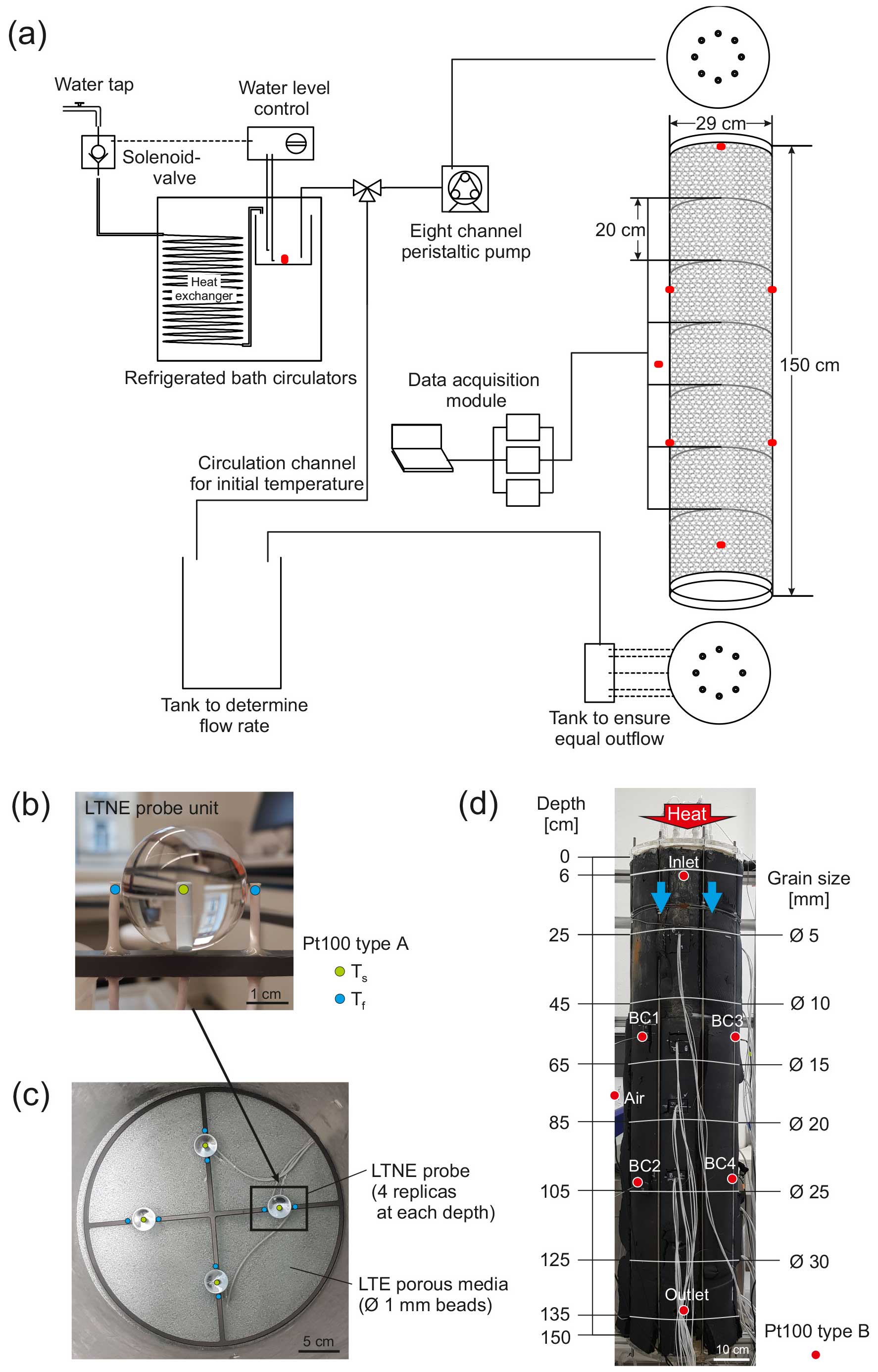
Figure 1 Overview of the experimental setup and its details: (a) conceptual diagram of the flow-through experiment; (b) LTNE probe unit, with the design of the LTNE probe showing one temperature sensor embedded within a sphere measuring the solid phase, as well as two sensors on each side measuring the fluid phase; (c) four replicas with the same grain size fixed on the PVC frame, with the arrangement of the hand-crafted LTNE probes, with four replicas for a specific sphere size, consisting of eight fluid temperature sensors and four solid temperature sensors for a specific depth; and (d) setup of the column filled with porous media and the LTNE probe arrangements for six different depths corresponding to six different grain sizes.

Temperature time series during the heat transport experiments were measured by two types of four-wire PT100 sensors. One type, referred to hereafter as PT100 type A, was a hermetically sealed resistance temperature detector with a diameter of 2 mm and an approximate resolution of ±0.01 °C, which was used to measure the temperature of fluid and solid phases (Fig. 1b). The other type, referred to hereafter as PT100 type B, was sheathed with a length of 18 cm and a diameter of 3 mm (Fig. 1d). It featured an accuracy of ±0.03 °C and was used for revealing boundary conditions. The temperature sensors were electronically controlled by 20 data acquisition modules, PT-104A (Omega Engineering Inc., USA), each with four channels at 1 s intervals (1 Hz measurement frequency), which is shown in Fig. 1a. The temperature response time of these devices was measured at approximately 4.7 s.

A total of 24 special LTNE probes were hand-crafted for six different glass sphere sizes (four for each diameter of 5, 10, 15, 20, 25, and 30 mm) to separately measure the temperature in the solid phase (at the center of the sphere) and on both sides of the surrounding fluid phase, as shown in Fig. 1b. For the solid-phase measurement, each glass sphere was designed to place a PT100 type A into the center of the sphere. Each glass sphere with a customized 2.5 mm hole was manufactured to be used as a grain in the experiments. Temperature sensors were carefully inserted and embedded using thermally conductive glue (thermal bonding system TBS20S, Electrolube, UK) with a thermal conductivity of 1.1 $\mathrm{W}{\mathrm{m}}^{-\mathrm{1}}{\mathrm{K}}^{-\mathrm{1}}$ and a volumetric heat capacity of 3.58 $\mathrm{MJ}{\mathrm{m}}^{-\mathrm{3}}{\mathrm{K}}^{-\mathrm{1}}$ to minimize heat transport influences. For the fluid-phase measurements, two temperature sensors were symmetrically placed next to each sphere at about 2 mm distance from the surface (Fig. 1b). Four replicas of each same-sized LTNE probe were fixed on a PVC frame with a thickness of 5 mm (Fig. 1c) and were placed at the specific depth in the column for one specific sphere size (Fig. 1d). These LTNE probes measured temperature development in time series. To determine LTNE effects, heat transport detected by a single probe unit (Fig. 1b) was considered in one experiment.

To stabilize the flow field surrounding the glass spheres, we embedded them in a porous medium consisting of water-saturated small-diameter glass beads (1 mm diameter) as, otherwise, fluid flow would be very sensitive to fluid dynamics or changes in density caused by the thermal front (i.e., free convection). This decision was based on experience with previous experimentation where a non-uniform flow field and associated anomalies challenged the analysis of transport parameters using temperature measurements (Rau et al., 2012a, b; Gossler et al., 2019). PT100 sensors for the fluid phase are embedded directly within small glass beads, without additional structure to separate them. While this setup may allow contact between the sensors and the beads, we assume that the fluid phases and solid phases of the small glass beads (d_p=1 mm) reach an instantaneous thermal equilibrium (LTE), resulting in identical temperatures. This design relies on the rapid thermal equilibrium established between the glass beads and water, which is justified by previous research (e.g., Gossler et al., 2019). This is also justified as it was demonstrated that LTNE should be negligible for grain diameters smaller than 7 mm (Gossler et al., 2020).

The small glass beads were filled above a perforated plate wrapped by filter fleece while the column was vertically positioned. The glass beads were manually packed in layers of 5–10 cm. Based on our experimental design, temperature sensors were located through new holes at the column to monitor the temperature breakthrough within the porous medium. During the packing, the hand-crafted LTNE probes were inserted within the porous media at different depths (i.e., distance along the flow path) along the column (Fig. 1d):

1. four 5 mm diameter spheres at 25 cm depth

2. four 10 mm diameter spheres at 45 cm depth

3. four 15 mm diameter spheres at 65 cm depth

4. four 20 mm diameter spheres at 85 cm depth

5. four 25 mm diameter spheres at 105 cm depth

6. four 30 mm diameter spheres at 125 cm depth.

The temperature was measured at the top (6 cm depth) and bottom (135 cm depth) of the column, and at the wall boundary, air temperature and inlet and outlet water temperature were measured to monitor boundary conditions (Fig. 1d). The porous media was filled slowly with water from the bottom upwards to displace air while avoiding trapped bubbles.

All temperature sensors underwent calibration within a water-filled bath placed inside the thermostat bath. Various temperature settings (5, 15, 20, 35 °C) were employed, and recordings were taken upon reaching the targeted temperature, ensuring the sensors had equilibrated. To establish a uniform initial temperature across the entire column, water circulation with the outlet water was employed. This process facilitated the equilibration of the temperature of porous media and fluid within the pores with the air temperature in the laboratory.

Upon achieving an initial temperature within the range of 24–30 °C through circulation, inflow commenced by switching a valve from the circulation channel to the inflow channel. The inflow, sourced from the laboratory tap, was preheated through a heat exchanger within the refrigerated bath, maintaining a temperature between 26–34 °C. The temperature of water in the bath was 5–8 °C higher than the initial temperature, which represents the equilibrated temperature of the system before the heat input was injected. Experimentation concluded when the temperature of all sensors reached a constant value at the culmination of the temperature rise.

Following the insights from Gossler et al. (2019) and their comprehensive testing of various column settings, we adopted the approach of conducting experiments in a vertically oriented column with a step heat input. This configuration yielded unbiased results by minimizing interference from free convection and guided our heat transport investigations. In our experimental setup, both water flow and temperature step input were introduced from the top to the bottom of the vertically positioned column. The heat input mechanism involved the injection of warm water from the top using a peristaltic pump, ensuring a constant flow rate and, consequently, a consistent Darcy flux within the column, ranging from 3 to 23 m d⁻¹. Subsequently, the outflow was discharged through tubes from the outflow tank connected to the bottom of the column (Fig. 1a). Flow rate quantification was achieved by weighing the collected outflow water on a minute-by-minute basis for each experiment.

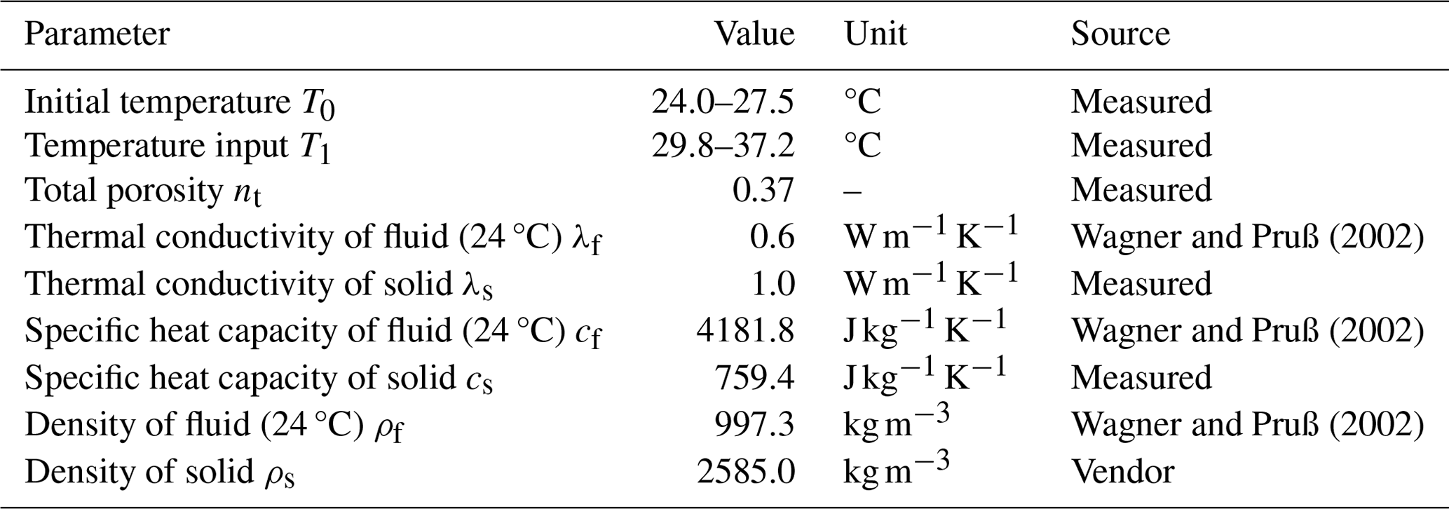
The total porosity of the porous media was determined experimentally. Glass beads, comprising the porous medium, were loaded and compacted into a cylinder with an inner diameter of 9.6 cm and a height of 12 cm to measure the weight of the beads. Using the weight derived from five repeated measurements of the packed cylinder, the calculated cylinder volume and the known density of the glass, the total porosity was calculated for each measurement and then averaged, yielding a result of 0.37. To ascertain the thermal conductivity and volumetric heat capacity of the glass (solid phase), the transient plane source (TPS) method was employed using a Hot Disk instrument (TPS 1500, C3 Prozess- und Analysentechnik, Germany). The measurements were conducted with the assistance of data acquisition software (Hot Disk Thermal Constants Analyser 7.4.17). The measurement uncertainties of the solid thermal conductivity λ_s and the solid volumetric heat capacity ρ_sc_s were 2 % and 7 %, respectively. The physical properties of both the fluid and solid phases are summarized in Table 1.

Wagner and Pruß (2002)Wagner and Pruß (2002)Wagner and Pruß (2002)

Table 1 Summary of parameter values of the porous medium, obtained from measurements or the literature.

2.2 One-phase model of heat transport in porous media

To describe heat transport during flow-through porous media representing an unconsolidated aquifer, the one-phase advection–diffusion heat transport equation is generally used in hydrogeological applications (Heinze, 2024). This assumes that the temperature of solid and fluid phases is always in equilibrium within an REV; hence, it is termed the local thermal equilibrium (LTE) model (Whitaker, 1991). The equation is as follows (de Marsily, 1986):

$$\begin{array}{}\text{(1)}& {\displaystyle }{\displaystyle \frac{\partial T}{\partial t}}=D{\displaystyle \frac{{\partial }^{\mathrm{2}}T}{\partial x^{\mathrm{2}}}}-v{\displaystyle \frac{\partial T}{\partial x}},\end{array}$$

where T is the temperature of the bulk porous medium (°C or K), t is the time (s), and x is the distance along the flow direction (m). The thermal-dispersion coefficient D (m² s⁻¹) is defined as (Rau et al., 2012a; Gossler et al., 2020)

$$\begin{array}{}\text{(2)}& {\displaystyle }{\displaystyle }D=\left({\displaystyle \frac{{\mathit{\lambda }}_{\mathrm{f}}}{{\mathit{\rho }}_{\mathrm{b}}{c}_{\mathrm{b}}}}+\mathit{\beta }{\left({\displaystyle \frac{{\mathit{\rho }}_{\mathrm{f}}{c}_{\mathrm{f}}}{{\mathit{\rho }}_{\mathrm{b}}{c}_{\mathrm{b}}}}q\right)}^{\mathrm{2}}\right)+{\displaystyle \frac{(\mathrm{1}-n){\mathit{\lambda }}_{\mathrm{s}}}{{\mathit{\rho }}_{\mathrm{b}}{c}_{\mathrm{b}}}}.\end{array}$$

The thermal conductivity of the saturated porous media is estimated by the arithmetic mean model as a mixing law model (Stauffer et al., 2013; Menberg et al., 2013; Tatar et al., 2021). This model leads to the maximum value of the thermal conductivity for glass packs, which is defined as follows:

$$\begin{array}{}\text{(3)}& {\displaystyle }{\displaystyle }{\mathit{\lambda }}_{\mathrm{b}}=n{\mathit{\lambda }}_{\mathrm{f}}+(\mathrm{1}-n){\mathit{\lambda }}_{\mathrm{s}},\end{array}$$

where n is the total porosity, and λ_f and λ_s are the thermal conductivities of the fluid and solid phases, respectively. Further, ρ_b is the density, and c_b is the specific heat capacity of the water-saturated porous media (bulk), which, when combined, represent the bulk volumetric heat capacity as (Buntebarth and Schopper, 1998)

$$\begin{array}{}\text{(4)}& {\displaystyle }{\displaystyle }{\mathit{\rho }}_{\mathrm{b}}{c}_{\mathrm{b}}=n{\mathit{\rho }}_{\mathrm{f}}{c}_{\mathrm{f}}+(\mathrm{1}-n){\mathit{\rho }}_{\mathrm{s}}{c}_{\mathrm{s}}.\end{array}$$

The fluid and solid densities are ρ_f and ρ_s (kg m⁻³), respectively; c_f and c_s are the specific heat capacities of the fluid and solid phases ($\mathrm{J}{\mathrm{kg}}^{-\mathrm{1}}{\mathrm{K}}^{-\mathrm{1}}$), respectively. The thermal-front velocity v is (Rau et al., 2012a)

$$\begin{array}{}\text{(5)}& {\displaystyle }{\displaystyle }v=q{\displaystyle \frac{{\mathit{\rho }}_{\mathrm{f}}{c}_{\mathrm{f}}}{{\mathit{\rho }}_{\mathrm{b}}{c}_{\mathrm{b}}}},\end{array}$$

where q is the Darcy velocity (m s⁻¹).

The LTE model (Eq. 1) was solved by an analytical solution as (van Genuchten and Alves, 1982)

$$\begin{array}{}\text{(6)}& {\displaystyle }{\displaystyle }\begin{array}{rl}{\displaystyle }{T}_{\text{norm}}& {\displaystyle }={\displaystyle \frac{T-T_{\mathrm{0}}}{T_{\mathrm{1}}-T_{\mathrm{0}}}}\\ {\displaystyle }& {\displaystyle }={\displaystyle \frac{\mathrm{1}}{\mathrm{2}}}\text{erfc}\left({\displaystyle \frac{x-v}{\mathrm{2}\sqrt{Dt}}}\right)+{\displaystyle \frac{\mathrm{1}}{\mathrm{2}}}\exp \left({\displaystyle \frac{vx}{D}}\right)\text{erfc}\left({\displaystyle \frac{x+vt}{\mathrm{2}\sqrt{Dt}}}\right),\end{array}\end{array}$$

with the following initial and boundary conditions:

$$\begin{array}{}\text{(7)}& {\displaystyle }& {\displaystyle }T=T_{\mathrm{0}}\text{ at all }\mathit{\text{x}}\text{ and }\mathit{\text{t}}=\mathrm{0},\text{(8)}& {\displaystyle }& {\displaystyle }T=T_{\mathrm{1}}\text{ at }\mathit{\text{x}}=\mathrm{0}\text{ and }\mathit{\text{t}}>\mathrm{0},\text{(9)}& {\displaystyle }& {\displaystyle }T=T_{\mathrm{0}}\text{ at }\mathit{\text{x}}=\mathrm{\infty }\text{ and }\mathit{\text{t}}>\mathrm{0}.\end{array}$$

Here, T_norm is the normalized temperature (–), T₀ is the initial temperature (K), and T₁ is the temperature (K) of heat input at the top boundary (x=0).

Equation (1) simplifies the heat transport description by considering the thermal energy in the porous medium as a bulk volume. This means it represents a volume-averaged temperature, as is reflected by the volume averaging of the thermal properties (Eqs. 2–4). We note that the thermal-dispersion coefficient D in this model incorporates both thermal diffusion through the two phases and hydrodynamic dispersion resulting from the flow-through tortuous flow paths. Experiments have demonstrated this to have a non-linear relationship with the flow velocity (Metzger et al., 2004; Molina-Giraldo et al., 2011; Rau et al., 2012a).

2.3 Two-phase model of heat transport in porous media

A more precise description follows from separating the temperature in the fluid and solid phases and considering heat transfer between the phases (Amiri and Vafai, 1994). This approach is termed local thermal non-equilibrium (LTNE). The fluid phase (subscript f) can be described as (Levec and Carbonell, 1985a; Kaviany, 1995)

$$\begin{array}{}\text{(10)}& {\displaystyle }{\displaystyle }n{\mathit{\rho }}_{\mathrm{f}}{c}_{\mathrm{f}}{\displaystyle \frac{\partial T_{\mathrm{f}}}{\partial t}}+{\mathit{\rho }}_{\mathrm{f}}{c}_{\mathrm{f}}v{\displaystyle \frac{\partial T_{\mathrm{f}}}{\partial x}}=n{\mathit{\lambda }}_{\text{f,eff}}{\displaystyle \frac{{\partial }^{\mathrm{2}}{T}_{\mathrm{f}}}{\partial x^{\mathrm{2}}}}+h_{\text{sf}}{a}_{\text{sf}}(T_{\mathrm{s}}-T_{\mathrm{f}}),\end{array}$$

whereas the solid phase (subscript s) is described by

$$\begin{array}{}\text{(11)}& {\displaystyle }{\displaystyle }(\mathrm{1}-n){\mathit{\rho }}_{\mathrm{s}}{c}_{\mathrm{s}}{\displaystyle \frac{\partial T_{\mathrm{s}}}{\partial t}}=(\mathrm{1}-n){\mathit{\lambda }}_{\text{s,eff}}{\displaystyle \frac{{\partial }^{\mathrm{2}}{T}_{\mathrm{s}}}{\partial x^{\mathrm{2}}}}-h_{\text{sf}}{a}_{\text{sf}}(T_{\mathrm{s}}-T_{\mathrm{f}}).\end{array}$$

Here, T_f and T_s are the separate temperatures of the solid and fluid phases, respectively. λ_f,eff and λ_s,eff are effective thermal conductivities of the fluid and solid phases, describing the thermal conductivity of each phase, with λ_f,eff for the fluid phase including hydrodynamic dispersion (Amiri and Vafai, 1994). These two energy equations are coupled by heat transfer between the fluid and solid phases, driven by the temperature difference between the solid and fluid phases and determined by the heat transfer coefficient h_sf ($\mathrm{W}{\mathrm{m}}^{-\mathrm{2}}{\mathrm{K}}^{-\mathrm{1}}$), as well as the specific surface area a_sf (m²). The heat transfer coefficient h_sf is the heat exchange across the surface area between the liquid and solid phases a_sf (m²), and these are defined as follows (Gossler et al., 2020):

$$\begin{array}{}\text{(12)}& {\displaystyle }& {\displaystyle }{h}_{\text{sf}}={\displaystyle \frac{\mathit{\text{Nu}}{\mathit{\lambda }}_{\mathrm{f}}}{d_{\mathrm{p}}}},\text{(13)}& {\displaystyle }& {\displaystyle }{a}_{\text{sf}}={\displaystyle \frac{\mathrm{6}(\mathrm{1}-n)}{d_{\mathrm{p}}}},\end{array}$$

where Nu is the Nusselt number, and d_p is particle (grain) size. The Nusselt number is a dimensionless parameter presenting the correlation between the heat transfer coefficient and hydraulic parameters. The correlation proposed by Wakao et al. (1979) is commonly utilized to estimate the heat transfer coefficient, which is derived from experiments in mechanical engineering (Kaviany, 1995; Amiri and Vafai, 1994; Bandai et al., 2023). While previous studies suggested different Nusselt number correlations from mechanical engineering, Gossler et al. (2020) proposed a general form of the Nusselt number correlation considering aquifer properties (Heinze, 2024). They suggested a correlation based on an adaptation of the Nusselt number by keeping the Prandtl number, a dimensionless parameter in the correlation of Wakao et al. (1979), constant for water at a fixed temperature. Although the correlation of Gossler et al. (2020) is experimentally not validated in porous aquifer conditions, it provides an estimation relevant to shallow groundwater flow regimes. Thus, the present study estimated the heat transfer coefficient by using the correlation of Gossler et al. (2020) and by fitting the LTNE model to the temperature difference between two phases from experimental data to achieve the best model for LTNE effects. The estimation of the heat transfer coefficient with the correlation with the Nusselt number Nu and the Reynolds number Re was performed with the following equations (Gossler et al., 2020):

$$\begin{array}{}\text{(14)}& {\displaystyle }& {\displaystyle }\mathit{Nu}=\mathrm{1}+\mathrm{3.1}{\mathit{\text{Re}}}^{\mathrm{0.57}},\text{(15)}& {\displaystyle }& {\displaystyle }\mathit{Re}={\displaystyle \frac{{\mathit{\rho }}_{\mathrm{f}}\left(q/n\right)d_{\mathrm{p}}}{\mathit{\mu }}}.\end{array}$$

Here, μ is dynamic viscosity ($\mathrm{kg}{\mathrm{m}}^{-\mathrm{1}}{\mathrm{s}}^{-\mathrm{1}}$), and d_p is the diameter of a grain (m).

The LTNE model (Eqs. 10 and 11) was solved in a one-dimensional space using FEniCS in Python (Alnaes et al., 2015). The model domain spans 1.5 m to represent the experimental setup used in our work. The equations are solved using the finite-element method with the following initial and boundary conditions (Bandai et al., 2023):

$$\begin{array}{}\text{(16)}& {\displaystyle }& {\displaystyle }{T}_{\mathrm{s}}=T_{\mathrm{f}}=T_{\mathrm{0}}\text{ for all }\mathit{\text{x}}\text{ and }\mathit{\text{t}}=\mathrm{0},\text{(17)}& {\displaystyle }& {\displaystyle }{T}_{\mathrm{s}}=T_{\mathrm{f}}=T_{\mathrm{1}}\text{ on }\mathit{\text{x}}=\mathrm{0}\text{ and }\mathit{\text{t}}>\mathrm{0},\text{(18)}& {\displaystyle }& {\displaystyle }{T}_{\mathrm{s}}=T_{\mathrm{f}}=T_{\mathrm{0}}\text{ on }\mathit{\text{x}}=\mathit{\text{L}}\text{ and }\mathit{\text{t}}>\mathrm{0}.\end{array}$$

Spatial and temporal discretizations were set at 0.5 mm and 1 s, respectively. Thermal breakthrough curves (BTCs) are generated for discrete distances of 0.2, 0.4, 0.6, 0.8, 1.0, and 1.2 m, corresponding to the temperature measurement points in the experimental setup for each grain size (Fig. 1d).

Equations (10) and (11) describe the heat flux for fluid and solid phases, respectively, allowing for temperature differences between the two phases. Accordingly, the effective thermal conductivity of each phase is considered in each energy equation to describe thermal conduction and dispersion phenomena (Amiri and Vafai, 1994; Bandai et al., 2023). The effective thermal conductivity λ_f,eff includes thermal diffusion in the fluid phase and hydrodynamic dispersion in relation to the flow velocity (Rau et al., 2012a). λ_f,eff was computed from the effective thermal conductivity λ_b of the porous media estimated by LTE model fitting experimental data. Optimization for the best fitting parameters, such as the effective thermal conductivity of the porous media λ_b and the heat transfer coefficient h_sf, was conducted using the Powell method from the SciPy package within the Python programming environment. The effective thermal conductivity of the solid λ_s,eff was considered to be the same as the thermal conductivity of the solid λ_s since thermal conduction of the solid phase is considered to be unaffected by the flow through.

2.4 Analysis of the experimental temperature measurements

To reveal possible LTNE heat transport effects, the temperature difference between the fluid and solid phases over time was calculated based on thermal BTCs for each LTNE probe. The temperature difference between the two phases was computed by subtracting solid-phase temperature from the adjacent fluid-phase temperature since heat transport was stimulated by inflow of heated water. The calculated temperature difference time series is referred to hereafter as ΔT(t), and values deviating from zero indicate temperature differences between the fluid and solid phases, indicating LTNE effects.

Although care was taken for each experiment to commence after thermal equilibration to the initial temperature within the column, slight variations in initial temperatures were observed among the sensors. The temperature difference between a pair of sensors within each LTNE probe unit was 0.05 K on average. This discrepancy could stem from sensor drift or calibration errors in the intercepts of the calibration curves. Since these discrepancies can obscure LTNE effects, a special data correction procedure was applied to all BTCs. The beginnings and tails of the breakthrough curves (BTCs) were adjusted to mitigate calibration errors of the sensors, making the plausible assumption that the initial and final temperatures were the same for each LTNE probe. The temperature records of the fluid and solid phases were normalized for each sensor in a time series by subtracting the initial temperature and then dividing by the temperature difference between the initial and final temperatures (equilibrated temperature at the tails of the BTCs) from the temperature measurement. The result of this is an upward or downward shift of the entire time series. This procedure allows for the evaluation of an improved ΔT(t) that is consistent and simple to interpret.

We further applied models to describe our experimental observations, assuming both LTE (Eq. 1) and LTNE (Eqs. 10 and 11) conditions. Here, the temperature measurements from the four probe replicas at the same depth (i.e., eight fluid temperature measurements and four solid temperature measurements, as shown in Fig. 1c) were averaged at each time step to represent fluid and solid temperature for each discrete distance along the flow path. The averaged temperature of fluid and solid phases allows data analysis with one-dimensional LTE and LTNE models.

3 Results

3.1 Solid and fluid temperature responses to inflow of heated water

Heat transport experiments revealed evidence of LTNE effects stemming from distinct thermal breakthrough curves (BTCs) for the solid and fluid phases over time. Figure 2 displays selected BTCs recorded within and next to a sphere for six different grain sizes in response to a temperature step input with Darcy flux values of 17.2 and 22.8 m d⁻¹. These BTCs, representing solid and fluid phases, are arranged according to increasing grain diameter, reflecting the expected behavior of heat transport: delayed arrival times for the solid phase and increased dispersion over distance.

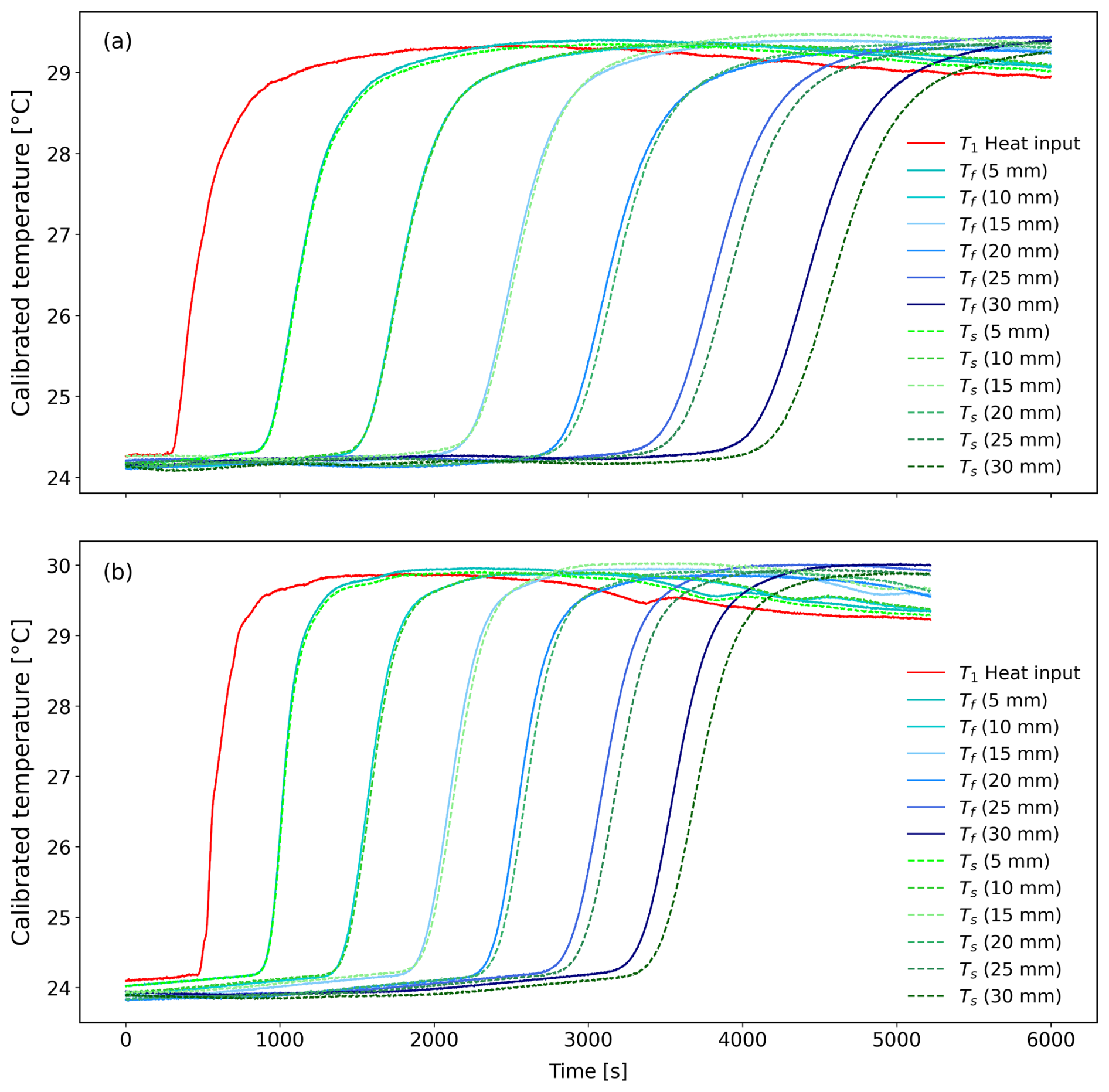
Figure 2 Calibrated temperature data yielded thermal breakthrough curves (BTCs) for both fluid and solid phases across six distinct grain sizes in heat transport experiments. The solid red lines present temperature measurements at the top of the column, indicating the temperature of heat input into the porous media. (a) The BTCs corresponding to a Darcy velocity of 17.2 m d⁻¹ exhibit variations in temperature between their initial and final states, as depicted in the plotted calibrated temperature measurements. (b) Conversely, the BTCs associated with a Darcy velocity of 22.8 m d⁻¹ illustrate a quicker attainment of equilibrium with the final temperature compared to those reflecting slower Darcy velocities.

A noticeable divergence between the fluid and solid BTCs becomes apparent with larger grain sizes, indicating temperature discrepancies between the two phases. An increase of calibrated temperature before the arrival of the thermal front was observed by the measurements at deeper depths for the larger grains. This may result from temperature variations during the equilibration phase, establishing a uniform initial temperature. Additionally, Fig. 2 shows that the calibrated temperature at 0 s varies between sensors, likely due to limited temperature control in the laboratory, which lacks air conditioning. The experimental procedure, necessitating the replenishment of the water bath with tap water during the experiment, is evident in the declining tails of the BTCs. However, as this replenishment occurred after the fluid and solid phases had equilibrated, it was deemed to be non-influential in our analysis.

3.2 Adjusted temperature breakthrough curves

The processed temperature data, based on measurements, are depicted in Fig. 3. This figure showcases temperature values from sensors at identical depths (Fig. 3a, c, and e) and the averaged temperature for both fluid and solid phases at those specific depths (Fig. 3b, d, and f) considering a Darcy flux of 22.8 m d⁻¹.

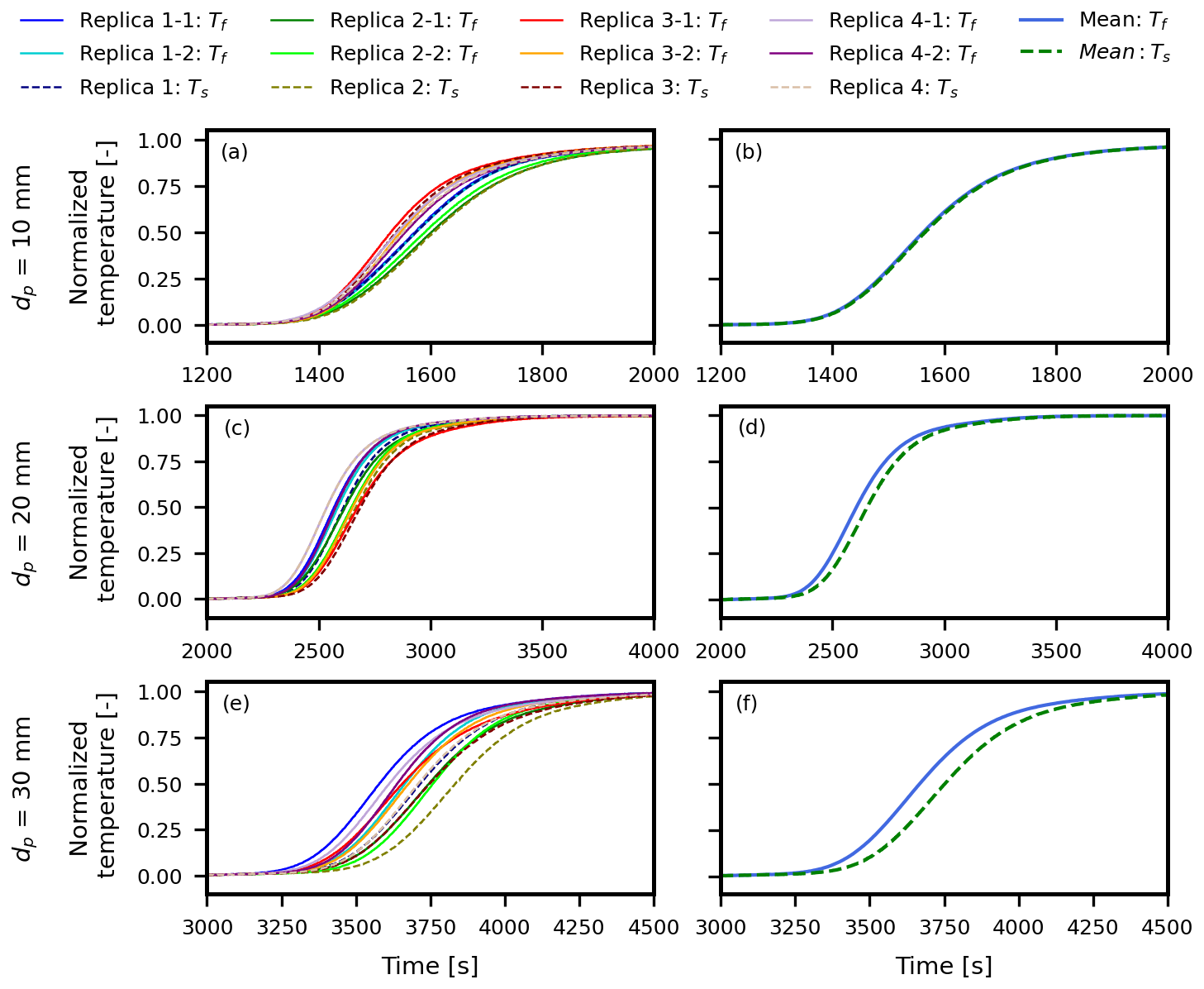
Figure 3 Thermal breakthrough curves (BTCs) derived from the processed data of temperature measurements (see Sect. 2.4) with a Darcy flux of 23 m d⁻¹, which shows the variation between measurements of LTNE probe replicas at the same depth. Here, T_f is presented as solid lines, while T_s is presented as dashed lines. The number (1 or 2) after the replica's number (1 to 4) indicates two different T_f measurements within an LTNE probe. (a, b) Corrected temperature measurements from all sensors and the averaged values of the corrected temperature for 10 mm grain at depths of 45 cm are presented. (c, d) For 20 mm grain, corrected temperature measurements at a depth of 85 cm, with deviations between all sensors, and their averaged values, including the delay of thermal arrival in the solid phase, are illustrated. (e, f) For 30 mm grain as the largest tested grain, corrected temperature measurements, with deviations among sensors of each phase, and the averaged temperature, with more pronounced deviations between the fluid and solid phases, are presented in comparison to (a–d).

As a result of the data post-processing, the thermal breakthrough curves (BTCs) exhibit a temperature rise from a consistent initial temperature, which is induced by heat input. Furthermore, the tails of the BTCs reach a uniform final equilibrated temperature for sensors at the specific depth corresponding to a particular grain size d_p. However, despite the identical flow velocity, the BTCs of each phase at the same depth display non-alignment due to varying thermal velocities, which depend on the transversal position of the LTNE probe (Fig. 3a, c, and e). Consequently, averaging the temperatures for the fluid and solid phases is necessary to obtain a representative temperature response for each phase at a given grain size and depth (Fig. 3b, d, and f).

In Fig. 3, the BTCs with the averaged solid temperature illustrate deviations from the averaged fluid temperature for the same grain size d_p, consistently with the findings from single temperature measurements of solid and fluid phases in an LTNE probe.

3.3 Temperature differences between phases

The temperature contrast between solid and fluid phases, as indicated by adjusted thermal breakthrough curves (BTCs), unveils the impact of varying grain size and flow velocities on the extent of LTNE effects. In Fig. 4, BTCs for both fluid and solid phases, along with their corresponding LTNE effects (ΔT(t)), are demonstrated for each grain size at the highest tested Darcy velocity of 23 m d⁻¹. This example highlights the maximum ΔT(t) observed among pairs of fluid and solid measurements for the same grain size. The disparity between fluid and solid BTCs signifies a delayed response in the solid phase, distinctly revealing the LTNE effect.

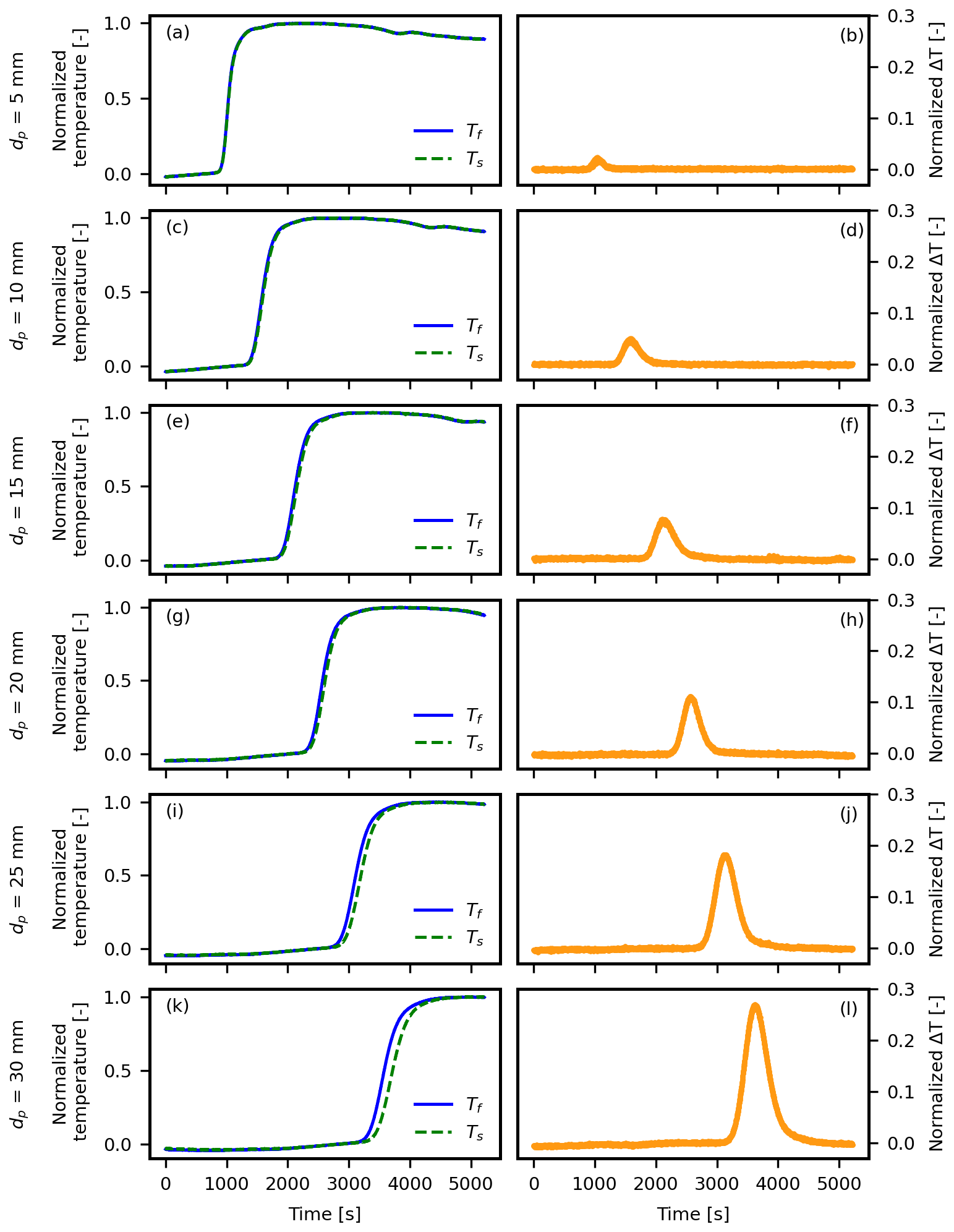
Figure 4 Thermal breakthrough curves (BTCs) of solid and fluid phases and ΔT(t) derived from experimental data with the maximum ΔT(t) among pairs of fluid and solid measurements in LTNE probe replicas with a Darcy flux of 22.8 m d⁻¹. (a, c, e, g, i, k) Thermal BTCs of fluid and solid phases for each grain size. It is clear from these panels that the deviation between BTCs of T_f and T_s becomes larger with increasing grain size. (b, d, f, h, j, l) ΔT(t) for each grain size. These present an increase in ΔT(t) peaks with increasing grain sizes.

The results showcase an augmentation of the maximum ΔT(t), reflecting an amplification of the LTNE effect with increasing grain size. Nevertheless, for grain sizes ranging between 5 and 15 mm, an “inverse pulse” of ΔT(t) was observed in some pairs of solid and fluid measurements across all tested flow velocities, as depicted in Fig. 5. This negative ΔT(t) arises from the solid phase exhibiting an earlier thermal response compared to the fluid phase, suggesting potential influences of a non-uniform flow field, resulting in different arrival times of the thermal front on both sides of the grain. Figure 5 shows that the normalized ΔT(t) patterns from two pairs within an LTNE replica (i.e., measurements from the same sensor positions) vary when the flow velocity changes. Additionally, the temperature differences between fluid-phase measurements from two sides of a sphere demonstrate changing patterns with varying flow velocity, suggesting different thermal-front arrivals in the fluid phase depending on the position near the sphere at the same depth.

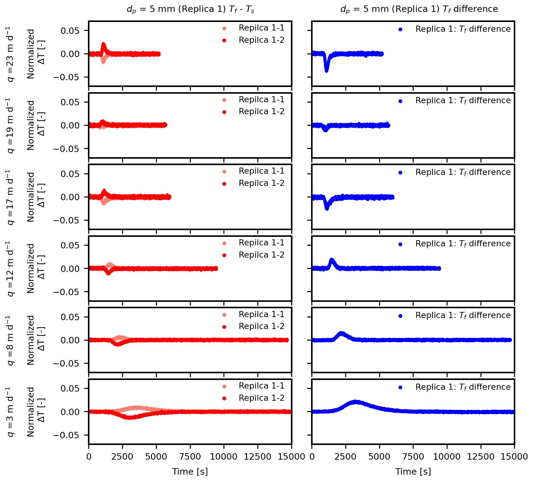
Figure 5 Experimental data from one of the LTNE probe replicas for 5 mm grain size with varied flow velocities, showing temperature differences between fluid and solid phases in time series as normalized ΔT(t), as well as temperature difference between two fluid phases measured next to a sphere in the probe. The change in the pattern of normalized ΔT(t) from the same measurement location is shown in this figure, implying that the non-uniform flow effects could influence the results for each experimental run.

In Fig. 6, the LTNE effect is displayed for each of the six sphere sizes across all flow velocities. These ΔT(t) curves represent examples of pairs of fluid and solid measurements showcasing the highest maximum ΔT(t). In general, the LTNE effect is intensified with larger sphere sizes. Moreover, increasing velocities exhibit a consistent trend across all spheres, characterized by a heightened peak with an earlier arrival time and a narrower spread of ΔT(t). This observation offers compelling evidence of LTNE, facilitating the exploration of its relationship with grain size and flow velocity.

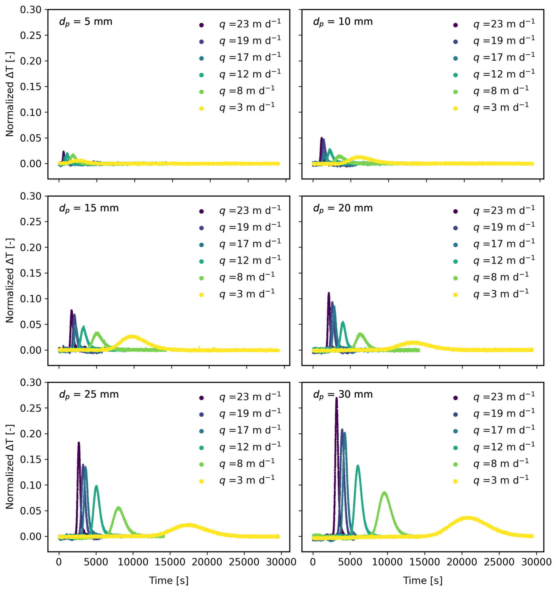
Figure 6 Summary of ΔT(t) curves from experimental data with all tested grain sizes from 5 to 30 mm diameter and Darcy velocities from 3 to 23 m d⁻¹. ΔT(t) curves are presented for each grain size with all tested Darcy velocities to compare the results with ΔT(t) curves of different grain sizes.

Figure 7 shows the quantitative evaluation of LTNE effects derived from the experimental data in relation to the grain size and flow velocity, based on the classification approach proposed in previous studies (Amiri and Vafai, 1994; Wang and Fox, 2023). The magnitude of LTNE effects can be determined by comparing the maximum normalized temperature differences. This can be expressed as follows: (Wang and Fox, 2023):

$$\begin{array}{}\text{(19)}& {\displaystyle }{\displaystyle }\text{LTNE }\left[\mathit{\%}\right]=\mathrm{100}\times {\displaystyle \frac{max\mid \mathrm{\Delta }T\left(t\right)\mid }{T_{\mathrm{1}}-T_{\mathrm{0}}}}.\end{array}$$

This quantified LTNE is classified into three categories: quasi-LTE, <5 %; low LTNE, 5 %–10 %; and LTNE >10 % (Fig. 7). This allows us to compare LTNE effects from experiments where different boundary temperatures were applied. The results demonstrate that the LTNE effects become significant when flow velocity is >12 m d⁻¹ for larger grain sizes (>20 mm).

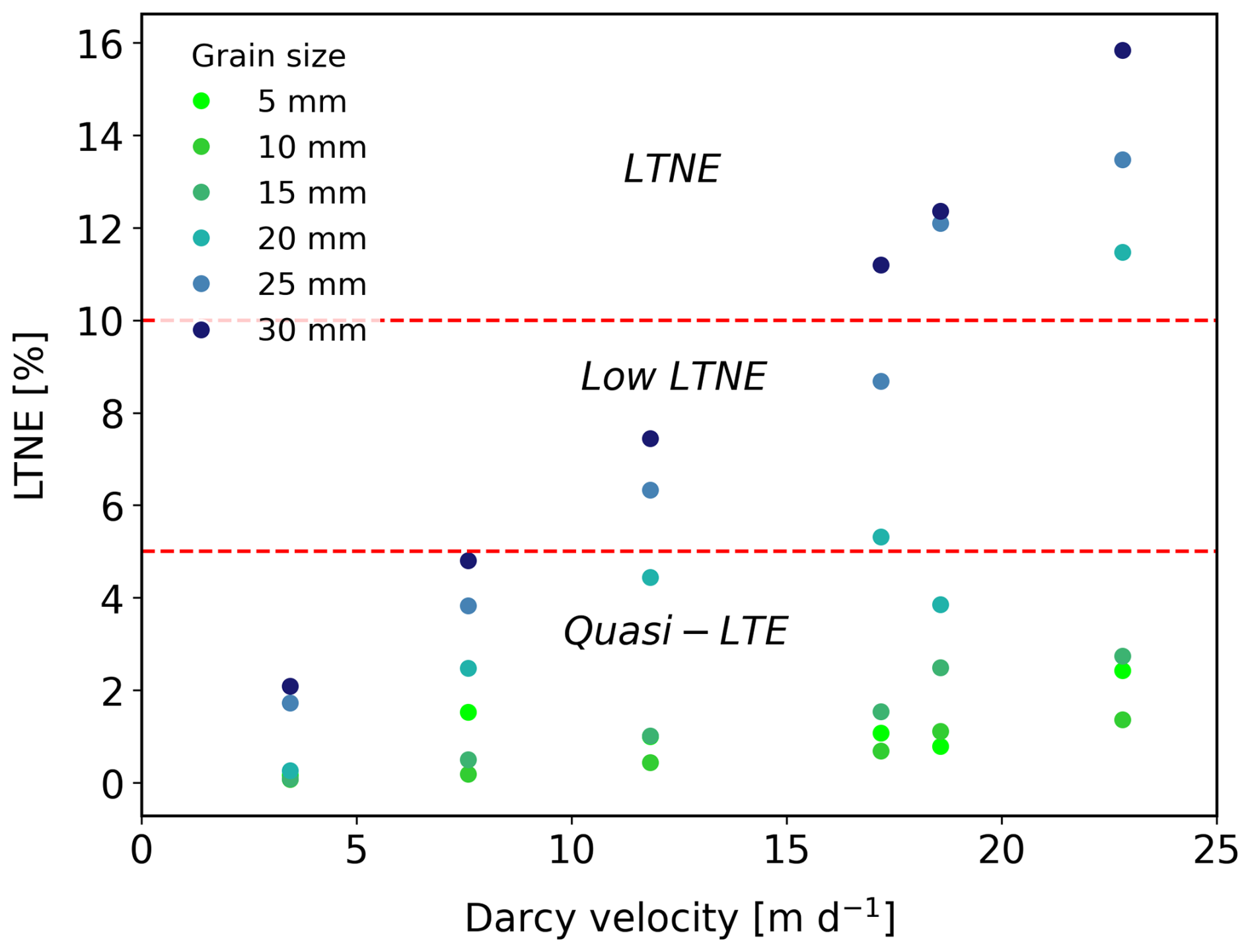
Figure 7 Quantitative evaluation of LTNE effects demonstrating the influence of grain sizes and flow velocities based on three categories: quasi-LTE, <5 %; low LTNE, 5 %–10 %; and LTNE >10 %. The dashed red lines indicate the lower limit for low LTNE (5 %) and LTNE (10 %). Experimental data for grain sizes ≥20 mm and Darcy velocities ≥12 m d⁻¹ revealed LTNE above 5 %.

3.4 Measured and modeled temperature breakthrough curves

The LTE analytical model exhibits limitations in predicting fluid temperature. This is particularly evident with larger grain sizes (≥20 mm) and faster flow velocities (≥12 m d⁻¹). Besides this, it successfully models BTCs of measured fluid-phase temperature for grain sizes of 5 and 10 mm, except for the tails of the BTCs. Notably, slower flow velocities (17 m d⁻¹) result in a better fitting of modeled BTCs to experimental BTCs, as shown in Fig. 8a and b. However, discrepancies between measured fluid temperature and model predictions become more pronounced for the 15 mm grain size, especially at faster flow velocities (23 m d⁻¹), as illustrated in Fig. 8c and d. For grain sizes ranging between 20 and 30 mm, the LTE model can only predict the beginning of the fluid-phase BTCs across all tested flow velocities.

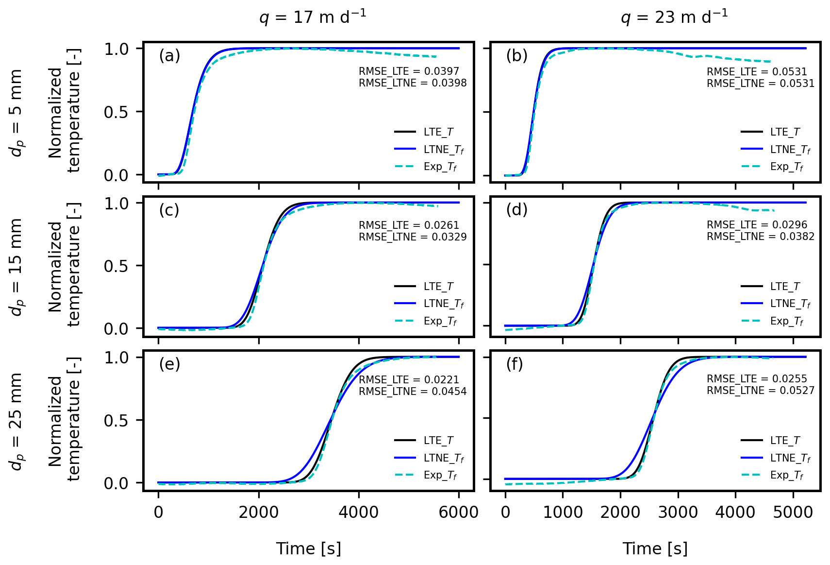
Figure 8 Comparison of LTE model, fluid-phase results from the LTNE model, and experimental data across all grain sizes with Darcy velocities of 17.2 and 22.8 m d⁻¹.

The LTNE model, on the other hand, offers improved predictions for the tails of BTCs from experiments due to the larger spread of LTNE BTCs compared to LTE BTCs. While the LTNE numerical solution aligns well with the tails of BTCs from experiments at a flow velocity of 23 m d⁻¹, it displays an early rise at the beginning of the curves and relatively better fitting at the end of the curves for slower flow velocities, as depicted in Fig. 8e and f.

The LTNE model demonstrated effective fitting to experimental BTCs and their corresponding LTNE effects for small grain sizes ranging from 5 to 15 mm, as depicted in Fig. 9. However, for grain sizes between 20 and 30 mm, the modeled ΔT(t) exhibited broader curves compared to experimental results. In the figure, LTNE model outcomes with h_sf estimated by Eqs. (12)–(15) (shown as dash-dotted green lines) exhibited relatively good agreement with ΔT(t) curves from experiments for a grain size of 5 mm, regardless of flow velocities (Fig. 9a and b). However, for grain sizes of 10 and 15 mm, the model overestimated ΔT(t) for all tested flow velocities, while it underestimated ΔT(t) for grain sizes ranging from 20 to 30 mm.

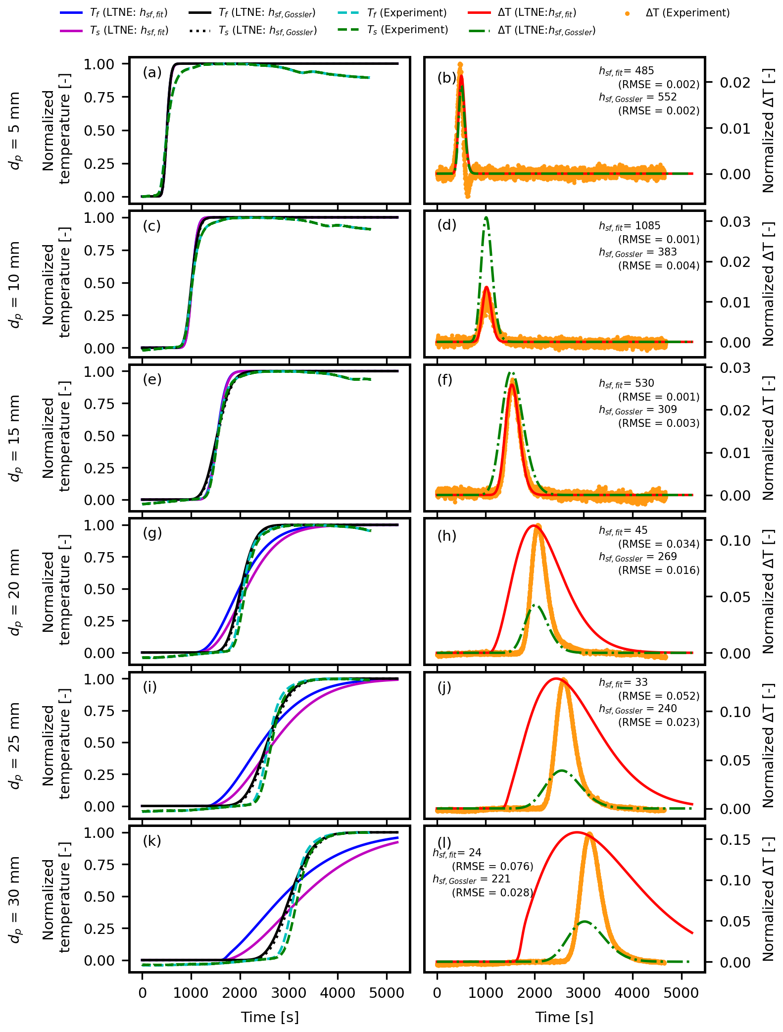
Figure 9 Comparison of experimental data with LTNE model outcomes using varied h_sf for all tested grain sizes at the highest flow velocity (23 m d⁻¹). LTNE model was simulated with the estimated h_sf by means of the correlation of Gossler et al. (2020), h_sf,Gossler, and by means of fitting to the experimental data, h_sf,fit. (a, c, e, g, i, k) Thermal breakthrough curves (BTCs) of fluid and solid phases for six different grain sizes derived from experiments and two LTNE model outcomes with h_sf,Gossler and h_sf,fit. (b, d, f, h, j, l) ΔT(t) for six different grain size from LTNE model with h_sf,Gossler and h_sf,fit. The estimated h_sf value for each model is presented for each grain size.

Nevertheless, the LTNE model successfully predicted the maximum ΔT(t) when the heat transfer coefficient was varied as a fitting parameter for all tested grain sizes and flow velocities, as depicted by the red lines in Fig. 9. However, for grain sizes between 20 and 30 mm, the LTNE model with fitted h_sf struggled to match the BTCs and the spread of corresponding ΔT(t) curves from experiments (Fig. 9h, j, and l).

4 Discussion

4.1 Experiments reveal local thermal non-equilibrium heat transport

Our work utilized four separate LTNE probes at each distance along the flow path to capture the spatial variability of heat transport processes, thereby enhancing the interpretation of the experimental findings. By conducting separate temperature measurements for both fluid and solid phases, we were able to discern the transient temperature disparities between these phases as ΔT(t). This demonstrated the occurrence of LTNE across various grain sizes (from 5 to 30 mm) and flow velocities (from 3 to 23 m d⁻¹) in a range between 0.018 and 1.577 K, which is beyond the temperature sensor accuracy range of ±0.01 K. While our observations are made for novel conditions, they align with the definition of LTNE by Kaviany (1995) that is characterized by considerable temperature differences between fluid and solid phases compared to the fluid temperature difference over the system during advective heat transport in porous media.

The LTNE effects observed in our experiments confirm limited observations from previous experiments on heat transport in porous media with water flow. For example, by measuring fluid and solid temperatures separately, Levec and Carbonell (1985b) showed a delayed thermal-pulse arrival in the solid phase for urea formaldehyde spheres (ρ_sc_s = 0.002 $\mathrm{MJ}{\mathrm{m}}^{-\mathrm{3}}{\mathrm{K}}^{-\mathrm{1}}$, λ_s = 1 $\mathrm{W}{\mathrm{m}}^{-\mathrm{1}}{\mathrm{K}}^{-\mathrm{1}}$), with a size of 5.5 mm. However, their work did not include an analysis of the temperature difference between the two phases. With a similar two-phase temperature measurement approach, Bandai et al. (2023) demonstrated ΔT(t) derived from the temperature difference between two phases for 5 mm glass spheres. Bandai et al. (2017) revealed the influence of particle size on thermal dispersion by means of heat transport experiments with small glass spheres (0.4, 1 and 5 mm). While LTNE effects were determined without solid temperature measurements by estimating the effective thermal retardation factor when comparing solute and heat tracer experiments (Gossler et al., 2019; Baek et al., 2022), this approach does not allow for transient assessments and is therefore limited to qualitative determination of LTNE. Our study confirms LTNE effects under groundwater flow conditions and provides the ability to quantitatively determine transient LTNE effects as ΔT(t) in a relation to the grain sizes and flow velocities.

ΔT(t) was analyzed from all fluid and solid measurement pairs by subtracting the solid from the fluid temperatures. Due to the delayed thermal arrival of the thermal signal in the solid phases, ΔT(t) is expected to be positive always. However, negative ΔT(t) values resulting in a significant inverse pulse, with a minimum between −0.31 and −0.04, were observed at some measurement locations for small grain sizes between 5 and 15 mm (Fig. 5). The inverse pulse may be attributed to the non-uniform flow and/or uncertainties in sensor positioning. While we cannot rule out sensor position uncertainties, our results showed that the thermal fronts measured by the sensors at the same location varied with changes in flow velocity. This phenomenon of non-uniform flow was previously reported by an experimental observation when multiple temperature sensors were used at the same discrete locations along the flow path (Rau et al., 2012b). Non-uniform flow causes the thermal front to propagate non-uniformly in the transversal direction, i.e., perpendicularly to the flow direction. This means that local thermal velocities at the thermal front are different. In our case, non-uniform flow causes the thermal front to arrive at different times on both sides of a sphere, leading to the solid response being faster than the fluid response on the side with slower velocity. The result is a negative ΔT(t), hereafter referred to as an inverse pulse. The occurrence of this phenomenon for smaller grain sizes suggests that this flow non-uniformity may either occur at small scales and/or be spread out through transverse dispersion over the travel distance, disallowing detection. Notably, inverse pulses of ΔT(t) were not observed for grain sizes of 20–30 mm, suggesting that non-uniform flow may have a stronger impact on results with smaller grain sizes owing to the smaller representative elementary volume (REV).

Previous studies that conducted experiments with separate temperature measurements for the two phases demonstrated that LTNE effects were limited to grain sizes ≤5.5 mm (Levec and Carbonell, 1985b; Bandai et al., 2023). In the study of Bandai et al. (2023), temperatures for fluid and solid phases were separately measured, and the maximum normalized temperature difference between fluid and solid phases for 4.94 mm glass spheres with a thermal conductivity of 0.76 $\mathrm{W}{\mathrm{m}}^{-\mathrm{1}}{\mathrm{K}}^{-\mathrm{1}}$ was up to 0.04 at a Darcy velocity of 29 m d⁻¹. In comparison, our study showed a smaller maximum normalized temperature difference of 0.02 between the two phases for 5 mm spheres with a lower Darcy velocity of 23 m d⁻¹. The smaller LTNE effects observed in our results may be attributed to the dependence of LTNE on Darcy velocities as Bandai et al. (2023) demonstrated that LTNE effects increase with higher Darcy velocities. While a similar pattern appears in our findings, some LTNE probes displayed ΔT(t) with peaks near zero or with inverse values (Fig. 5). These results could be due to non-uniform flow degrading the magnitude of ΔT(t) compared to uniform flow. The same mechanism could also cause LTNE effects with a stronger magnitude due to local differences in the thermal velocity surrounding the sphere as a result of non-uniform flow effects. Having four replicas for each sphere size provides the advantage of capturing the variability and allowing a more robust assessment of LTNE.

The experimental data were generated using a specially designed setup to examine the influence of varying grain sizes on heat transport under different flow conditions. Drawing on insights from prior studies (Rau et al., 2012a; Gossler et al., 2019; Bandai et al., 2023), we crafted our setup to effectively measure the temperature difference between fluid and solid phases. This setup allows for efficient experimentation with 2 degrees of freedom (grain size and velocity) within a single configuration. By incorporating all six different grain sizes into one experiment, we were able to test identical flow velocities across different grain sizes, which is challenging to achieve in separate experiments. The grain sizes were arranged in increasing order along the depth of the column because of the evolution of the thermal front. Since the steepness of the thermal front decreases as heat moves downward, the smallest grain size, which is expected to exhibit smaller LTNE effects (Gossler et al., 2019), was placed at the top, where the gradient is steepest, and, progressively, the larger grain sizes were positioned at greater depths. At each depth, the solid-phase temperature for four LTNE probe replicas was measured at the center of the glass spheres to represent solid temperature. Measuring temperature at the surface of the glass spheres was technically challenging due to the sensor's thickness and the limited contact area with each sphere. Similar challenges and inconsistencies in surface temperature measurements for the solid phase were reported by Bandai et al. (2023) in their heat transport experiments. Therefore, this study assumes that the temperature at the center of the spheres accurately represents the solid-phase temperature, disregarding any internal temperature gradient within the spheres.

4.2 Local thermal non-equilibrium increases with grain size and velocity

Using ΔT(t) as a measure for transient LTNE allows for detailed insights into the heat transport processes. Our results clearly show that LTNE effects increase in magnitude with grain sizes ranging from 5 to 30 mm and Darcy velocities ranging from 3 to 23 m d⁻¹. The wider ΔT(t) peaks observed at slower flow velocities indicate that it takes longer to achieve thermal equilibrium between the two phases with lower flow velocities. Furthermore, for Darcy velocities ranging from 3 to 23 m d⁻¹, the magnitude of ΔT(t) grows up to about 10 times a 5 mm grain size with increasing grain size, showing the stronger LTNE effects with larger grain sizes for all tested flow velocities.

While inverse pulse of ΔT(t) were observed for 5–15 mm grain sizes across all tested flow velocities, the maximum ΔT(t) in the experiments tended to be higher than the minimum ΔT(t) in the inverse pulse. Notably, the magnitude of LTNE effects for the smallest grain size of 5 mm remains smaller than 0.2 K for all tested flow velocities. This illustrates that the influence of flow velocities on LTNE for the smallest grain size of 5 mm was not clearly evident in our study, which aligns with recent theoretical investigations hypothesizing that LTNE effects should not occur for grain sizes smaller than 7 mm (i.e. for sand and fine gravels) (Gossler et al., 2020).

We note that Baek et al. (2022) identified LTNE effects for a grain size as small as 0.76 mm but with fast Darcy velocities that exceed 20 m d⁻¹. However, they did not directly measure solid and fluid temperatures but instead established LTNE by comparing solute with heat transport. In our study, no significant increase in LTNE effects was observed for a 5 mm grain size. This discrepancy could be attributed to the heterogeneity of porous media in different grain sizes and shapes, as reported by Baek et al. (2022).

4.3 Simplified heat transport models insufficiently describe local thermal non-equilibrium

We replicated our experimental observations using LTE and LTNE models, which led to mixed results. While the LTE model can be adjusted to fit near the beginning of breakthrough curves (BTCs) by varying the thermal velocity and dispersion coefficient, this fails to adequately model the entire BTC, including both the beginning and the tail. Bandai et al. (2023) also conducted heat transport experiments measuring fluid and solid phases separately and observed that the tail of BTCs from the fluid phase were more spread out compared to the LTE model, likely due to a non-ideal step heat input. While our temperature measurements from the top of the porous media exhibited steep BTCs in Fig. 2, they differed from the ideal step input (Heaviside step function) required to comply with the model's boundary conditions. This may lead to a misrepresentation of heat transport parameters as a result of misfitting.

The LTNE model was utilized to predict the magnitude of LTNE effects, determined by ΔT(t). The maximum ΔT(t) can be adjusted by varying the heat transfer coefficient as a fitting parameter in the model. The estimation of the heat transfer coefficient by means of the correlation of Gossler et al. (2020) was unable to model the maximum ΔT(t). This could be caused by the empirical relationship between Nusselt number Nu and Reynolds number Re used to derive the heat transfer coefficient. Consequently, the empirical Nu could lead to overestimation and underestimation of ΔT(t) by changing the spread of modeled BTCs. Our modeling results show that the 1D LTNE model closely describes the temperature difference between the fluid and solid phases for grain sizes of 5 and 10 mm (Fig. 9). However, for a grain size of 15 mm, deviations from experimental breakthrough curves (BTCs) become larger. For larger grain sizes ranging from 20 to 30 mm, the deviations become significant, and the LTNE model is unable to accurately predict ΔT(t). When optimizing the fitting of the maximum ΔT(t) by adjusting the heat transfer coefficient, the BTCs of the model deviate further from the experimental BTCs, deteriorating the fitting (Fig. 9g, i, and k). This limitation may be attributed to the constraints of the 1D model, specifically not capturing the multi-dimensional processes as caused by non-uniform flow, which was evidenced earlier. Additionally, the LTNE model is limited to describing the heat transfer between fluid and solid phases by means of a constant heat transfer coefficient (h_sf) without spatially distinguishing the phases and grain sizes.

Overall, non-uniform propagation of the thermal front caused by non-uniform flow leads to temperature gradients in the transverse direction and influences the nature of thermal processes, such as the magnitude of ΔT(t). Unfortunately, such processes cannot be captured by a 1D LTNE model as this is limited to describing the heat transport in the flow direction only. This does not accurately represent the experimental setup and exact temperature measurement points for fluid and solid phases. Consequently, to determine transport parameters such as the heat transfer coefficient (h_sf) from our experimental datasets, more sophisticated LTNE models are required. This goes beyond the scope of our study and should be done in future work.

Menberg et al. (2013)Clauser (2021a)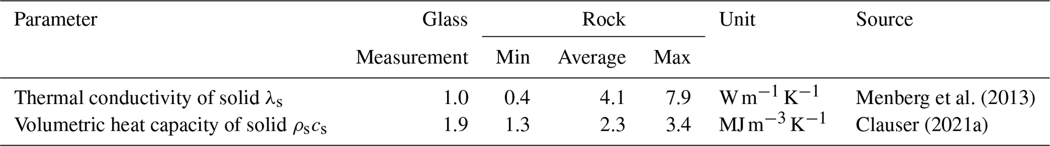

Table 2 Comparison between thermal properties of natural material (rock) from the literature (Clauser, 2021a, b) and experimental material (glass).

4.4 Implications for modeling heat transport in porous aquifers

Our experimental work confirms the presence of LTNE effects, prompting inquiry into their relevance to groundwater flow in aquifers. The glass spheres we employed possess a thermal conductivity of 1 $\mathrm{W}{\mathrm{m}}^{-\mathrm{1}}{\mathrm{K}}^{-\mathrm{1}}$ and a volumetric heat capacity of 1.9 $\mathrm{MJ}{\mathrm{m}}^{-\mathrm{3}}{\mathrm{K}}^{-\mathrm{1}}$. While these values may deviate from typical thermal parameters of groundwater systems, they fall within the reported range for natural sediments (Table 2). For instance, thermal-conductivity values range from 1 to 7.9 $\mathrm{W}{\mathrm{m}}^{-\mathrm{1}}{\mathrm{K}}^{-\mathrm{1}}$ for sedimentary rocks and quartz minerals, respectively (Clauser, 2021b; Menberg et al., 2013), and volumetric heat capacity values range from 2.3 to 3.6 $\mathrm{MJ}{\mathrm{m}}^{-\mathrm{3}}{\mathrm{K}}^{-\mathrm{1}}$ for impervious rocks and inorganic minerals, respectively (Banks, 2015; Clauser, 2021a). In the study by Bandai et al. (2023), they utilized an LTNE model to compute ΔT(t) across various values of thermal conductivity (ranging from 0.23 to 2.3 $\mathrm{W}{\mathrm{m}}^{-\mathrm{1}}{\mathrm{K}}^{-\mathrm{1}}$) and volumetric heat capacity in the solid phase (ranging from 1.0 to 4.18 $\mathrm{MJ}{\mathrm{m}}^{-\mathrm{3}}{\mathrm{K}}^{-\mathrm{1}}$). Their findings indicated that thermal conductivity does not significantly influence LTNE; i.e., the magnitude of ΔT(t) remains relatively stable. However, an increase in the volumetric heat capacity of the solid phase leads to heightened LTNE. This phenomenon occurs because the solid phase requires more energy to achieve a similar temperature rise. On the contrary, Gossler et al. (2020) theoretically demonstrated that the volumetric heat capacity of the solid phase exerts minimal influence on LTNE effects within an LTNE numerical model by means of parameter sensitivity analysis. To decipher the implications for real-world systems like porous aquifers, addressing this disparity demands the creation of sophisticated models that accurately represent the experimental heat transport processes.

Our experimental results are interpreted by using standard analytical and numerical models accepted in the literature. These models are commonly applied to explain heat transport in groundwater and to gain insights into thermal properties and processes. However, our results indicate that the LTE model cannot distinguish between the fluid and solid phases and is therefore limited to simplified heat transport scenarios without considering temperature differences between phases. Additionally, our simple 1D LTNE model failed to adequately represent the measured ΔT(t). The analysis revealed three main factors that were identified as limiting: (1) our measured BTCs likely did not comply with the ideal boundary condition (Heaviside step function) assumed by standard analytical solutions, (2) the occurrence of non-uniform flow caused inverse pulses and may therefore also contribute to variations in ΔT(t) that cannot be captured by simple models, and (3) LTNE heat transport appears to be a multi-dimensional process with geometrical effects. This clearly highlights the limitations of simplified heat transport models in estimating thermal parameters and capturing advanced heat transport processes based on experiments. We suggest that future studies should focus on developing advanced numerical models capable of incorporating a greater level of detail. These models should be adopted to analyze experimental data and provide deeper insights into the intricacies of heat transport processes.

Our study directly measures thermal disequilibrium between fluid and solid phases (i.e., LTNE effects) at the granular scale, offering insights into the conditions under which LTNE effects arise and may impact larger scales. However, further research is needed to connect findings from grain-scale applications to field-scale applications. This heat transport experiment focused on the influence of grain size and flow velocity on LTNE, addressing a critical gap in the scientific literature. While our results are representative for porous media with uniform grain sizes, future research should investigate LTNE effects in porous media with realistic grain size distributions.

5 Conclusions

We conducted systematic laboratory experiments on heat transport by subjecting water flow to temperature step inputs at Darcy velocities ranging from 3 to 23 m d⁻¹ through porous media composed of idealized spherical grains, with diameters between 5 and 30 mm. Temperature breakthrough curves (BTCs) were separately measured in the fluid and solid phases. Our results unequivocally demonstrate transient local thermal non-equilibrium (LTNE) heat transport effects, characterized by a temporary temperature discrepancy ΔT(t) between the two phases over time. This discrepancy indicates that the solid phase exhibits a time lag compared to the fluid phase in response to passing thermal transience. Importantly, we observed that the LTNE effect becomes more pronounced with increasing grain size (5–30 mm) and Darcy velocity (3–23 m d⁻¹), aligning with previously unverified theoretical predictions. Furthermore, negative temperature differentials between the solid and fluid phases for smaller grains (5–15 mm) were attributed to non-uniform flow inducing transverse temperature gradients.

To reconcile experimental observations and to estimate heat transport parameters, we employed both an analytical solution, assuming local thermal equilibrium (LTE) heat transport, and a numerical solution to the transient local thermal non-equilibrium (LTNE) differential equations, both of which are state of the art and are conducted in one-dimensional space. The LTE and LTNE models exhibit relatively good agreement with the breakthrough curves (BTCs) observed in the fluid phase for small grain sizes ranging from 5 to 15 mm, demonstrated by an RMSE $<\mathrm{0.01}.$ However, for larger grain sizes (≥20 mm), the LTE model fails to adequately describe heat transport, primarily due to significant LTNE effects with ΔT(t) larger than 5 % of the system temperature gradient, violating LTE criteria as defined in Sect. 3.3 and Fig. 7. Additionally, discrepancies between the models and experimental data with regard to the tails of BTCs for large grains suggest that the experimental conditions may not align with the boundary conditions assumed in the solution. Analysis of the experimental data using the LTNE model yields successful results only for small grain sizes within the range of 5–15 mm, while the model struggles to accurately capture transport behavior for larger grain sizes (≥20 mm), such as coarse gravels.

The experimental findings from this study provide experimental evidence for grain-size- and velocity-dependent transient local thermal non-equilibrium (LTNE) effects that was postulated theoretically. However, a comprehensive comparison between experimental data and models reveals only partial success. Several factors contribute to this discrepancy: (1) non-ideal boundary conditions, deviating from the assumed step-like conditions in standard analytical solutions, are present in the experiments. (2) Non-uniform flow induces inverse temperature gradients, altering ΔT(t) and complicating the interpretation of properties from BTCs. (3) State-of-the-art one-dimensional models lack the capacity to fully capture the multi-dimensional nature of LTNE heat transport processes.

Future research endeavors should prioritize the development of sophisticated two-phase numerical models capable of analyzing the experimental dataset comprehensively, enabling the derivation of advanced heat transport processes and properties.