Probabilistic downscaling of EURO-CORDEX precipitation data for the assessment of future areal precipitation extremes for hourly to daily durations

This work presents a methodology to inspect the changing statistical properties of precipitation extremes with climate change. Data from regional climate models for the European continent (EURO-CORDEX 11) were used. The use of climate model data first requires an inspection of the data and a correction of the biases of the meteorological model. Corrections to the biases of the point precipitation data and those of the spatial structure were both performed. For this purpose, a quantile–quantile transformation of the point precipitation data and a spatial recorrelation method were used. Once corrected for bias, the data from the regional climate model were downscaled to a finer spatial scale using a stochastic method with equally probable outcomes. This allows for the assessment of the corresponding uncertainties. The downscaled fields were used to derive area–depth–duration–frequency (ADDF) curves and areal reduction factors (ARFs) for selected regions in Germany. The estimated curves were compared to those derived from a reference weather radar dataset. While the corrected and downscaled data show good agreement with the observed reference data over all temporal and spatial scales, the future climate simulations indicate an increase in the estimated areal rainfall depth for future periods. Moreover, the future ARFs for short durations and large spatial scales increase compared to the reference value, while for longer durations the difference is smaller.

1 Introduction

Climate change became a very important issue in the past decades. It is likely to affect life conditions all over the world. One of the important issues in this context is how magnitudes and frequencies of extremes will change. A large number of studies were conducted to investigate this issue. In general, global climate models (GCMs) are used to model the past changes (forced by observations) in climate systems on a global scale and to project future changes (forced by emissions scenarios) (Randall et al., 2007). These are based on the numerical solution of mathematical representations of the physical processes and their interactions (such as the conservation of energy, mass, and momentum; the thermodynamic equations such as the gas laws; and the connection of processes on land to the atmosphere and vice versa) (Randall et al., 2007; Hennemuth et al., 2017). A GCM provides output variables with relatively coarse space-time resolutions, typically between 100 and 500 km² and for 6 h intervals (Stocker, 2014). However, the transfer and use of global results to local and regional climate analysis, especially for hydrological processes such as precipitation, require a finer space-time resolution, which can be achieved through downscaling. The latter can be divided into two categories: empirical-statistical downscaling (ESD) and dynamic downscaling via regional climate models (RCMs) (Rummukainen, 2010). ESD exploits the statistical nonlinear relationships between small- and large-scale information about climate variables. RCMs use the GCM output as lateral boundary conditions, and, coupled with parameterization schemes to account for local aspects (e.g., topography), climate data are acquired at a higher spatial resolution. Depending on the driving GCM and the applied parameterization schemes, several RCM ensembles are available (Kotlarski et al., 2014). Although GCM and RCM data provide essential information about climate systems, they cannot fully and correctly simulate all relevant spatial and temporal processes. Representative concentration pathways (RCPs) provide information about possible future climate scenarios (Nakicenovic et al., 2000). The change in emission concentration is integrated into the GCM calculations and converted into carbon dioxide (CO₂) equivalents. An increase in the amount of greenhouse gases implies an increase in the global temperature and, hence, an alteration of the climatic system (Van Vuuren et al., 2011; Pachauri et al., 2014). In the case of the Coordinated Downscaling Experiment for the European Domain (Euro-CORDEX CMIP5) data, the governing GCM is driven by a set of several RCP scenarios (Nakicenovic et al., 2000), with RCP8.5 being the scenario with the largest increase in greenhouse gas emissions by the end of the 21st century. Due to the increase in temperature values, the maximum amount of water vapor in the atmosphere increases, which leads to an increase in the frequency and intensity of precipitation extremes (Li et al., 2021). However, the rate of increase is not exactly known, and the change varies spatially and temporally (Singh, 2017).

Despite the ongoing advancement of RCMs, their immediate applicability is fraught with challenges, including the existence of biases compared to observational data (e.g., frequency of occurrence of dry and wet values, precipitation intensity in extreme events, wet and dry spatial patches, and systematic underestimation or overestimation), limitations in the spatial resolution (discrepancies in the model and observation spatial scales), and the correct representation of the spatial dependence structures between the different locations. Kotlarski et al. (2014) found that precipitation values from different hourly RCM datasets, even at seasonal and regional scales, exhibit a bias of ±40 % with a tendency for overestimation. Meredith et al. (2021) examined the precipitation diurnal cycle for current and future periods of EURO-CORDEX. Most models exhibit timing errors in the occurrence of maximum hourly precipitation intensities. In all models, the peak occurred several hours before the one appearing in the observations. Several methods have been developed to reduce the bias in regional climate model (RCM) simulations. Teutschbein and Seibert (2012) provided an overview of several bias correction methods, indicating that even simple approaches were able to mitigate the biases in the model data. Moreover, Maraun (2013) illustrated that bias correction methods based on quantile mapping of the cumulative distribution functions (CDFs) of different spatial scales (e.g., points and grid cells) are a deterministic approach that results in a misrepresentation of the temporal and spatial variability. For reliable results, bias correction methods should be applied using reference data at the same spatial scale as the model data. However, even the most sophisticated bias correction methods cannot handle large model errors and, if used incorrectly, can lead to false climate change signals (Maurer and Pierce, 2014; Maraun et al., 2017). To overcome these problems, so-called trend-preserving approaches have been developed, which aim to maintain the trends in the mean and in the higher quantiles (Hempel et al., 2013; Casanueva et al., 2020).

Lange (2019) and Volosciuk et al. (2017) suggested treating the bias correction and downscaling parts separately. Bias adjustment should be performed at the same spatial scale between observations and the climate model output. Downscaling climate model data to a finer spatial resolution (namely, bridging the scale gap), should then be done using a stochastic rather than deterministic approach (e.g., interpolation) (Maraun, 2013). Furthermore, Widmann et al. (2019) compared the resulting spatial variability of multiple downscaling methods and found that only the techniques that considered a multi-site behavior or directly modeled the spatial dependence gave a realistic representation of the spatial dependence structure. Bárdossy and Pegram (2012) analyzed the spatial dependence of bias-corrected RCM daily precipitation values and showed how it is underestimated. The effects of the underestimation were clearly noticeable at larger spatial scales and led to an underestimation of areal precipitation extremes. To address this, the authors introduced a recorrelation approach to correct the model dependence structure. Switanek et al. (2022) implemented a stochastic downscaling scheme based on temporally and spatially corrected RCM daily data to transfer the coarse-scale RCM data to a finer scale and derive spatially coherent daily precipitation time series.

Concerning the change in the frequency and intensity of precipitation extremes, an increase is projected, especially for sub-daily durations (Westra et al., 2014; Cannon and Innocenti, 2019; Fowler et al., 2021). However, Berg et al. (2019) examined the derivation of summer depth–duration–frequency (DDF) statistics from hourly EURO-CORDEX data at the highest available horizontal resolution (EUR-11) for several European countries (including Germany). National DDF reference curves were used for comparison. Several RCMs were selected; the quality was considered fair for the long duration, but the models showed poor representation of the hourly extreme values for the short duration. The rainfall amount corresponding to a 10-year return period was greatly underestimated by the RCM outputs. The problem lies in the way convection is represented. The latter plays a major role in sub-grid processes and sub-daily rainfall extremes. A newer family of models, the convection-permitting models (CPMs), running at a finer horizontal resolution (≤4 km), show a better representation of the hourly precipitation extremes (Meredith et al., 2021; Ban et al., 2021). However, additional development is required due to several biases being present, and the high computational requirements limit their current large-scale applications (Kendon et al., 2014; Berthou et al., 2020). Several approaches were proposed to derive future DDF curves (or adapt current DDF curves) from RCM precipitation data. Martel et al. (2021) provided an overview of current methods. The first line of thinking consists of modifying current DDF curves by a constant or a variable increase factor. The simple constant percentage increase method applies a constant increase factor (between 15 % and 30 %) to current DDF values. An alternative is the adaptive percentage increase method that utilizes an increase factor that is dependent on the projected temperature increase and rainfall frequency for future periods. The factor changes for the different durations and return periods. Another approach is the percentage increase based on the Clausius–Clapeyron relationship, which relates the change in rainfall intensity to the local increase in temperature (°C⁻¹). All of the aforementioned methods were based on upscaling of current DDF curves to future ones. Other methods, however, exist that utilize the outputs of GCMs and RCMs. For example, Srivastav et al. (2014) derived future DDF curves using GCM data for the region of Canada by an equidistant quantile mapping of the annual maxima. Spatial downscaling was used to transfer the data to the point scale, and temporal downscaling was used to account for the changes between the historical and RCP future projections. Mantegna et al. (2017) used data from a dynamical and high-resolution convection-parameterizing RCM to derive sub-daily intensity–duration–frequency (IDF) curves. The latter were compared to two observation locations in Australia. The future IDF curves suggest an increase in sub-daily rainfall intensities of 15 % °C⁻¹. So et al. (2017) derived future IDF curves for South Korea from daily RCM data through stochastic downscaling to sub-daily resolutions, which was incorporated into a Bayesian inference framework. The results indicate an increase in the expected rainfall from 5 % to 30 % under the RCP8.5 scenario. Other studies also exist; for example, Hosseinzadehtalaei et al. (2018) derived future IDF curves for Belgium, Forestieri et al. (2018) derived them for Sicily (Italy), and Khazaei (2021) derived them for Iran.

Many of the previous studies considered deriving the DDF (or IDF) for the point scale. Traditionally, areal reduction factors (ARFs) are used to transfer the point value to the areal (or catchment) scale. These are in general based on simple assumptions, and the effect of climate change is not considered. However, the consequences of heavy precipitation, such as flooding, are related to the volume of water, so the spatial aspect should not be ignored. This work considers precipitation as a spatial phenomenon, without purely point statistics, and aims to assess the expected change in future areal precipitation extremes under the RCP8.5 scenario compared to reference data and the present period. This is done by calculating area–depth–duration–frequency (ADDF) curves over several durations (hourly to daily) and over different spatial scales from 1 to 1000 km². Essential questions to be investigated in this work are the following:

1. Knowing that precipitation extremes look different depending on scales, to what extent can the climate model produce extremes correctly?

2. How can spatial and temporal dependence structures of climate models be successfully corrected?

3. How will the statistics of areal extremes change with climate projections?

To answer these questions, the following scheme was undertaken. The first step consisted of upscaling the point data to the model scale. This enabled us to derive a reference for temporal and spatial dependence structures. A recorrelation procedure was implemented to correct the model spatial dependence structure to match the reference. In the second step, the bias in the magnitudes of future projections and any subsequent bias in the marginal distribution function was corrected using a double-QQ (quantile–quantile) transformation. The corrected data at the model scale were then spatially downscaled using the random-mixing conditional simulation method (Bárdossy and Hörning, 2016). From the downscaled spatial fields, areal precipitation statistics were derived and compared to those extracted from weather radar data. The downscaling and analysis of areal precipitation extremes are showcased in the Sect. 3 of this paper. The results are discussed, and a conclusion involving key messages finalizes the paper.

2 Study area and data description

The study area is delimited by the weather radar region of Hanover, located in the state of Lower Saxony in Germany. The weather radar is positioned at the Hanover Airport and has a coverage radius of 128 km. The north of the region is generally flat, and moving toward the southeast the elevation increases to 1141 m a.s.l. in the Harz Mountains. The average yearly precipitation ranges from 500 to 1700 mm yr⁻¹ (Haberlandt and Berndt, 2016b). Following previous studies on the space-time statistics of rainfall extremes, the weather radar region of Hanover was selected as the study area (El Hachem, 2023). Within this region, the German Weather Service (DWD) operates a precipitation measurement network of 127 rain gauges with sub-hourly resolution (DWD Climate Data Center, 2021a). The data for these stations were acquired for the years between 2005 and 2020. Moreover, the hourly weather radar data (RADOLAN, Radar-Online-Aneichung) for the period 2005–2020 were used. RADOLAN is the operational DWD radar composite and is a merged product of the derived precipitation fields from all available weather radars and the DWD rain gauges. The data were made available by the DWD (DWD Climate Data Center, 2021b). For this study, only the observations lying within the radar area of Hanover were extracted. The third dataset is the EURO-CORDEX data. These have been provided within the Coordinated Regional Downscaling Experiment (CORDEX) for the European continent with two horizontal simulation domains of 50 km (EUR-44) and 12.5 km (EUR-11). The simulation output consists of several datasets with hourly resolution, representing different atmospheric and near-surface variables such as precipitation (Jacob et al., 2014). The REgional MOdel (REMO) is especially advantageous for precipitation analysis at the hourly scale since advection is integrated within the parameterization scheme (Jacob and Podzun, 1997; Jacob, 2001). In this work, the MPI-M-MPI-ESM-LR-GERICS-REMO2015-v1 data developed by the Max-Planck-Institut für Meteorologie (MPI-M) and the Climate Service Center Germany (GERICS) were used. The data were made available by the ClimXtreme Central Evaluation System framework (Kadow et al., 2021).

Figure 1 presents the locations of the EURO-CORDEX 11° center grid points in Germany and in the radar area of Hanover (black circle). To avoid edge effects in the interpolated and simulated fields, only model points falling within a 10 km inward buffer (red circle) of the radar coverage boundary were selected. The DWD rain gauges are visualized as orange triangles. The magenta points in the lower right map present the centers of the radar pixels. The weather radar grid with a spatial resolution of 1 km constitutes the interpolation and simulation grid. The orange box is a 12.5×12.5 km polygon presenting one EURO-CORDEX grid cell (centered around the green point). In total, 273 grid cells are available within the selected area.

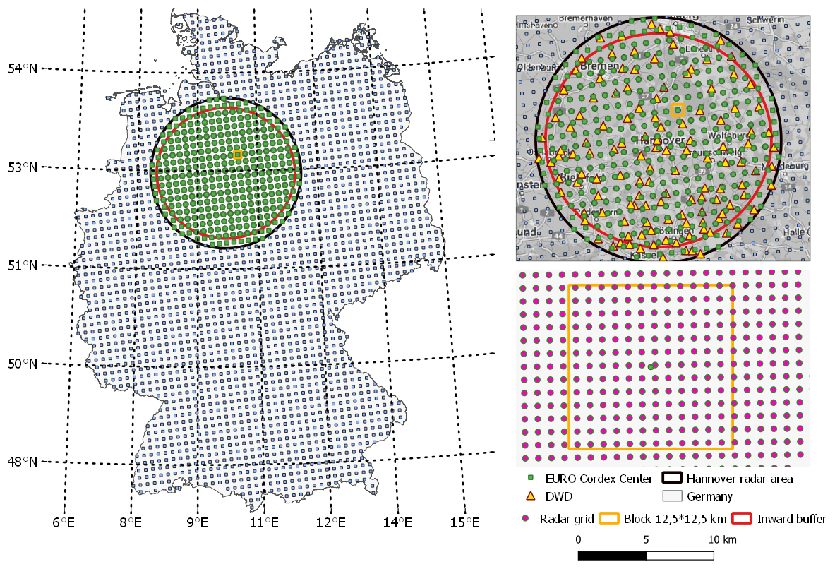
Figure 1 Map of Germany with the EURO-CODEX 11° grid center locations. The study area is shown, defined by the weather radar area of Hanover along with the DWD rain gauge data and the radar grid. Background map © Google Maps.

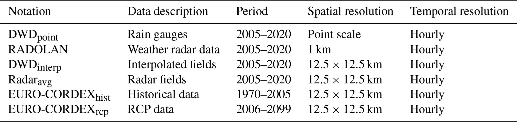
The goal is to find the reliability/usability of the RCM data for areal precipitation analysis with a special focus on extremes. Since the model data consist of grid cell averages, comparing them to rain gauge (point) data is unsuitable. Hence, the initial reference data were derived from interpolated fields utilizing the DWD station data, referred to as DWD_point. The interpolation was carried out using ordinary kriging, and the weather radar observation grid of 1 km was used as the interpolation grid. The resulting fields were then spatially aggregated to match the EURO-CORDEX 11° grid. This reference dataset will be denoted hereafter as DWD_interp. The second dataset is the spatially averaged radar data for the period 2005–2020. The aggregated data match the model grid and are denoted hereafter as Radar_avg. Note that in all cases the arithmetic mean of the 1 km pixels falling within each model cell was calculated and assigned to the corresponding model pixel. A summary of the datasets is presented in Table 1.

Table 1 Description of the datasets along their availability and corresponding spatial and temporal resolutions.

3 Methodology

The procedure for analyzing, correcting, and downscaling the RCM data is divided into three parts and is presented in Fig. 2. First, the spatial dependence structure of the model needs to be corrected according to a reference-based structure. The distribution of the point precipitation amounts is subsequently corrected. To mitigate the influence of the biased precipitation amount distribution on the spatial structure, the analysis was conducted using pixelwise rank correlation derived from a reference dataset, such as DWD_interp. This approach is more complicated than using a distance-based correlation structure. The reason for selecting this procedure is that, at this scale due to local (e.g., topographical) effects, the correlation structure is not homogeneous. The correction is based on a recorrelation procedure described in Sect. 3.1. The dependence structure greatly affects the areal extremes, especially for large spatial events (Bárdossy and Pegram, 2012). This section refers to part (a) of the flowchart in Fig. 2. After rectifying the dependence structure, it is essential to manage any remaining bias in the marginal distribution function of future climate projections. For this, a double-QQ transformation involving information from the reference data and the model historical data was applied (Bárdossy and Pegram, 2011). This section represents part (b) of the flowchart in Fig. 2. Afterwards, the final corrected data are downscaled using the random-mixing stochastic simulation algorithm (Bárdossy and Hörning, 2016) to the finer spatial resolution of 1 km. The final fields are eventually used for the analysis of the spatial extent of extremes via area–depth–duration–frequency (ADDF) curves. The ADDF curves were calculated on the pixel scale (1 km² area) for different areas (up to 1024 km²) and durations (hourly to daily). The possible impact of climate change on the statistics of areal extremes was investigated. Note that this section refers to part (c) of the flowchart in Fig. 2.

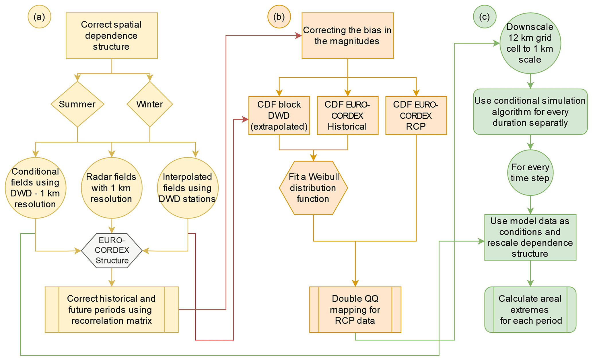
Figure 2 Flowchart describing the methodology for correcting the spatial (a) and temporal (b) structures of EURO-CORDEX 11° data. The corrected values are then downscaled (c) and used for analysis of areal extremes.

3.1 Correction to the dependence structure

The spatial dependence of precipitation plays a major role in the distribution of areal rainfall and the corresponding extremes. An often neglected problem is whether regional climate models can replicate the observed dependence structure. In Bárdossy and Pegram (2012), this problem was discussed, and a possible solution was presented. A similar procedure was implemented in this study but using finer spatial and temporal resolutions. Furthermore, instead of the Pearson correlation the Spearman correlation (rank correlation) was used with normal-score-transformed variables. To account for different precipitation mechanisms and characteristics, the reference and model data were divided between the summer (April–September) and winter (October–March) seasons, and for each period the dependence structure was derived. A special challenge while working with sub-daily and especially hourly precipitation data is the large number of 0 mm precipitation values (around 80 %).

Figure 3 displays the pairwise normal-score-transformed rank correlation values for each dataset individually plotted against the separating distance between each and every other grid cell. For the EURO-CORDEX data, the historical and future periods present similar behaviors, and only the historical data are displayed. Note that each correlation matrix has a size of 273×273 (the number of RCM grid cells). Panel (a) shows the correlation structure derived from the DWD rain gauges DWD_point (black dots) and the spatially averaged DWD_interp data (red dots). The DWD_point correlation values are lower than those of the DWD_interp data. This difference can be justified theoretically – assuming stationarity of the spatial dependence – as the interblock variability leads to a reduction of the variance. In fact, the covariance between two grid cells V_i and V_j can be written as a function of the covariance function of the point values C(x,y):

$$\begin{array}{}\text{(1)}& \text{Cov}(V_i,V_j)={\displaystyle \frac{\mathrm{1}}{\left|V_i\right|}}{\displaystyle \frac{\mathrm{1}}{\left|V_j\right|}}\underset{V_i}{\int }\underset{V_j}{\int }C(x,y)\mathrm{d}x\mathrm{d}y.\end{array}$$

For the variance of the grid cell V, we have the following:

$$\begin{array}{}\text{(2)}& \text{Var}\left(V\right)=\text{Cov}(V,V)={\displaystyle \frac{\mathrm{1}}{\left|V\right|\left|V\right|}}\underset{V}{\int }\underset{V}{\int }C(x,y)\mathrm{d}x\mathrm{d}y.\end{array}$$

Both the covariance and the variance decrease when comparing point to areal estimates. The decrease in the covariance is less than or equal to that of the variance, thus the correlation increases. Thus, due to scale difference, using the DWD_point correlation structure as a reference for the correction of the EURO-CORDEX spatial structure would be incorrect.

In panels (b) and (c), the red dots represent the DWD_interp, the blue dots the Radar_avg, and the orange dots the EURO-CORDEX data. Panel (b) shows the winter period, and panel (c) shows the summer period. The results for DWD_interp show a typical behavior of decreasing correlation with increasing separating distance associated with a large scatter. In both cases, the correlation structures of Radar_avg present a smaller scatter and fall below those of DWD_interp and EURO-CORDEX. In other words, Radar_avg shows less spatial continuity (a quick drop of correlation) and larger variability between the grid cells. Compared to DWD_interp, the EURO-CORDEX data show an underestimation of the dependence structure, especially in the summer period. The recorrelation method aimed to adjust the model dependence structure to match the reference over all temporal aggregations.

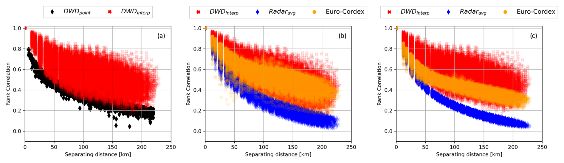
Figure 3 Panel (a) shows the rank correlation values between the DWD rain gauges (DWD_point) for the winter period (black dots) and between the DWD_interp grid cell values (red dots) for the same period. Panels (b) and (c) show the calculated grid cell pairwise rank correlation values from interpolated fields (red points), radar fields (blue points), and EURO-CORDEX fields (orange dots) for the winter and summer periods, respectively. The x axis refers to the separating distance between the grid cells. Note that the white vertical spaces are caused by the neighboring grid cells with a separating distance of ≈12.5 km.

The procedure presented by Bárdossy and Pegram (2012) used a mixed-type distribution, defined by a censored Gaussian copula, to transform the daily precipitation data to the normal space, and a matrix recorrelation procedure based on linear algebra was implemented. The aim was to recorrelate the model data to obtain the same reference dependence structure. The latter was derived by calculating the Pearson correlation between the daily precipitation time series at the different grid cell locations. A similar procedure was implemented in this section but using the correlation of the normal-score-transformed data.

A normal score transformation cannot be performed directly due to the large portion of zero values. Thus, instead, indicator series were used. The indicator series I(t,u) were calculated for the reference and model data, when given a probability level α. Several threshold values were tested, and the value α=0.9 was selected as it provided the best recorrelation results.

Let F(t,u) be the distribution function of the precipitation time series Z at location u. The indicator series can be calculated using Eq. (3). After converting the reference and model data to indicator series (either 0 and 1), the pairwise correlation between the two indicator series ρ_i(u,v) was calculated. The indicator correlation matrix is defined by R_i for the reference data and by M_i for the model data.

$$\begin{array}{}\text{(3)}& I(t,u)=\left\{\begin{array}{ll}\mathrm{1}& \text{if }F\left(Z\right(t,u\left)\right)>\mathit{\alpha },\\ \mathrm{0}& \text{else}.\end{array}\right.\end{array}$$

For a given probability level α, there is a one-to-one relationship between the indicator correlation (ρ_i(u,v)) corresponding to two locations u and v and the correlation of a bivariate Gaussian variable (ρ_g(u,v)) which has the same indicator correlation. Figure A2 displays this relation for different probability levels, and Eq. (4) describes it quantitatively.

$$\begin{array}{}\text{(4)}& {\mathit{\rho }}_{\mathrm{g}}(u,v)={\displaystyle \frac{\mathrm{1}}{\mathrm{2}\mathit{\pi }\mathit{\alpha }(\mathrm{1}-\mathit{\alpha })}}\underset{\mathrm{0}}{\overset{\mathrm{arc}\sin {\mathit{\rho }}_i(u,v)}{\int }}\exp \left({\displaystyle \frac{-y_{\mathit{\alpha }}^{\mathrm{2}}}{\mathrm{1}+\sin t}}\right)\mathrm{d}t\end{array}$$

Here, y_α is defined as the standard normal quantile corresponding to a probability α. The indicator and Gaussian correlations between the two locations u and v are represented by ρ_i(u,v) and ρ_g(u,v), respectively.

The estimation of ρ_g(u,v) has to be carried out numerically. Using the relation in Eq. (4), both indicator correlation matrices (describing the correlation between the grid points) of the reference and model data, R_i and M_i, were transformed to Gaussian correlation matrices R_g and M_g. To ensure that the correlation matrices for the grids, R_g and M_g, are positive and semi-definite, minor modifications to the correlation values were undertaken while minimizing the distance between the original matrices (R_g and M_g) and the modified matrices (${\mathbf{R}}_{\mathrm{g}}^{*}$ and ${\mathbf{M}}_{\mathrm{g}}^{*}$) (Bárdossy and Plate, 1992).

The flowchart in Fig. 4 gives an overview of the recorrelation steps as follows:

1. transform reference and model data to indicator series for every season separately using Eq. (3),

2. calculate the indicator correlation matrix of reference data R_i,

3. calculate the indicator correlation matrix of model data M_i,

4. transform R_i and M_i to Gaussian correlation matrices R_g and M_g using Eq. (4),

5. ensure that R_g and M_g are positive and semi-definite and modify them to ${\mathbf{R}}_{\mathrm{g}}^{*}$ and ${\mathbf{M}}_{\mathrm{g}}^{*}$,

6. decompose the correlation matrix ${\mathbf{R}}_{\mathrm{g}}^{*}$ by singular value decomposition (SVD) to obtain its square root matrix S_g,

7. decompose (SVD) the correlation matrix ${\mathbf{M}}_{\mathrm{g}}^{*}$ and calculate its inverse square root to obtain T_g (the matrix T_g decorrelates the model results; S_g is then transforming the decorrelated values to the desired correlation),

8. calculate the recorrelation matrix F=S_gT_g by matrix multiplication,

9. recorrelate the model data M to ${\mathbf{M}}^{*}=\mathbf{MF}$ by matrix multiplication,

10. transform the M^* values back to precipitation using the corresponding marginal distributions.

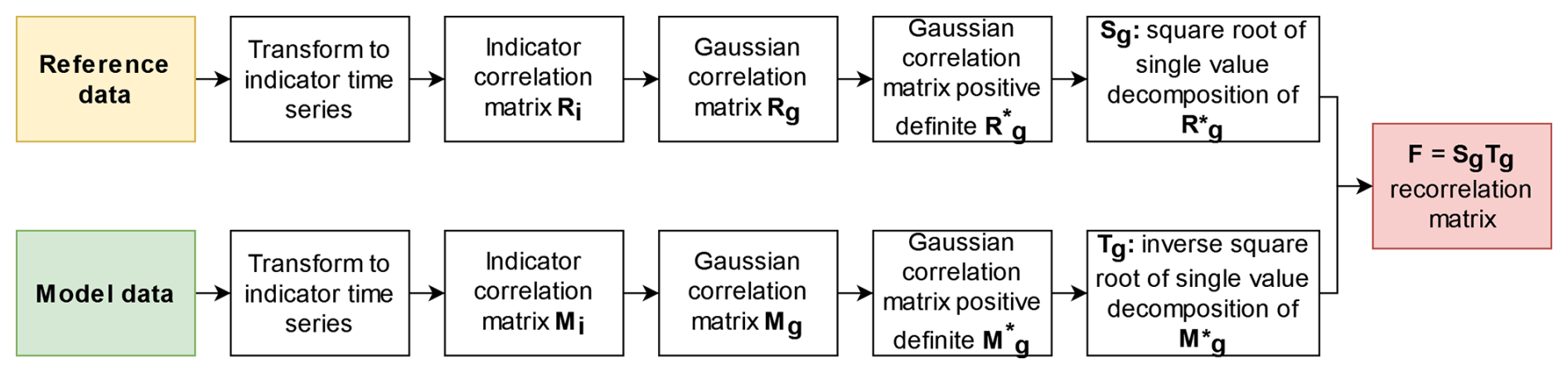
Figure 4 Flowchart describing the methodology for recorrelating the EURO-CORDEX data to have a similar dependence structure as the reference data.

The correction procedure should correct the dependence structure of the modeled precipitation. As dependence can be measured with different statistics, a set of possibilities is shown in Fig. 5. In all panels of Fig. 5, the x axis and the y axis values refer to the reference and model data correlation values, respectively. In panel (a), the blue points represent the indicator correlation values, namely, the matrices R_i and M_i. In panel (b), the red dots are the correlation values after the normal score transformation, and the green and blue dots are those after the correction of the spatial structure. The Pearson and rank correlations between the reference and model data were calculated and are presented in panels (c) and (d), respectively. In panel (c), the original Pearson correlation values (black points) showcase an improvement after the correlation procedure (orange points). Meanwhile, in panel (d), the rank correlation values show an improvement after the correction (points in green). Similar results were obtained for the winter period.

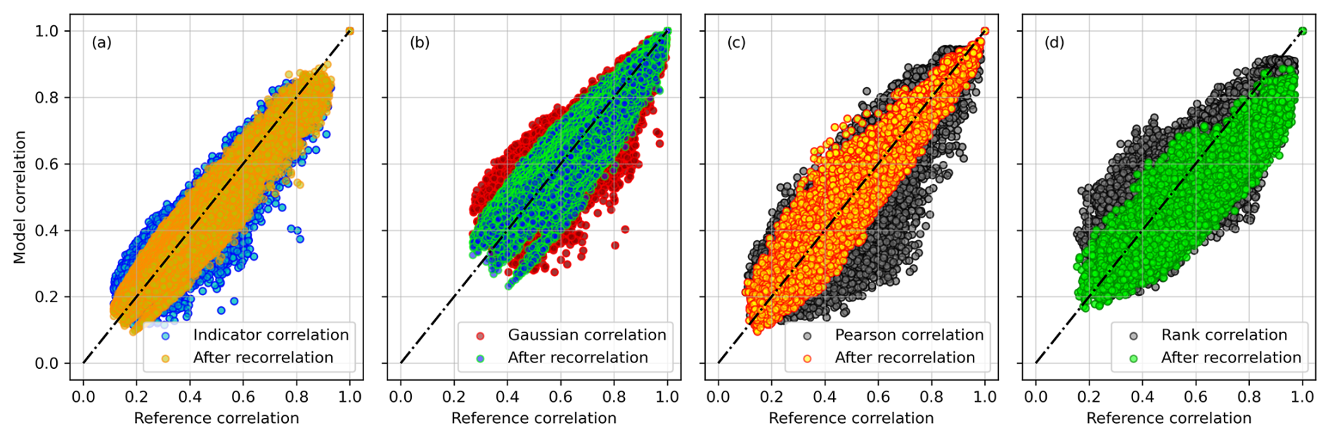
Figure 5 Panel (a) shows the indicator correlation values between the reference DWD_intep (x axis) and the EURO-CORDEX data (y axis) before correction (blue dots) and after correction (yellow dots). In panel (b), the Gaussian correlation values are displayed before correction (red dots) and after recorrelation (green and blue dots). In panel (c), the Pearson correlation values before (black and gray dots) and after recorrelation (orange and yellow dots) are shown. In panel (d) the rank correlation values before (black and gray dots) and after recorrelation (green dots) are displayed. The reference and model dependence structures were calculated for the summer period.

The recorrelation matrix F derived from the historical observations for each season separately can be used to recorrelate projected RCP scenarios. This is possible since the model's historical and future dependence structures are highly similar (see Fig. A1). In Fig. 6, the correlation values of the original and recorrelated grid cells are calculated and compared to reference values. The correlation values of the EURO-CORDEX_hist are displayed by the black dots (before recorrelation) and the red dots (after recorrelation) in panel (a) for the winter period and in panel (b) for the summer period, respectively. The results indicate that the recorrelation procedure improved the model dependence structure compared to the observed DWD_interp (x axis) data for both seasons.

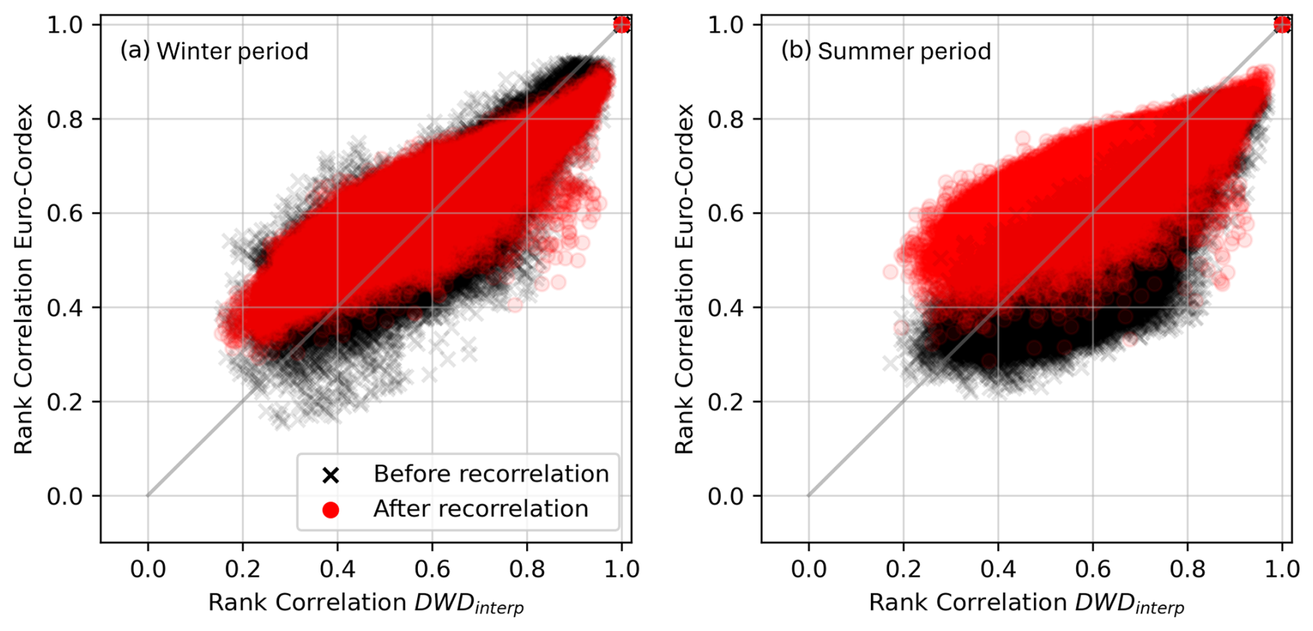
Figure 6 Panels (a) and (b) show the calculated grid cell pairwise rank correlation values for the winter and summer periods from DWD_interp (x axis) and EURO-CORDEX_hist fields (y axis). The dots in black and in red refer to the rank correlation of the EURO-CORDEX fields before and after recorrelation, respectively.

The recorrelation procedure was done for every duration (from hourly to daily) separately. This provided consistent results for all durations. Note that this complete section refers to part (a) of the flowchart in Fig. 2. After correcting the dependence structure, the marginal distribution function of the model's future data was corrected using a double-QQ transformation.

3.2 Double-quantile–quantile mapping

In statistics, quantile–quantile plots (QQ plots) are used to compare two distributions and identify if they both belong to the same distribution function. Often a test distribution is compared to a theoretical one. The comparison is based on the quantiles. Namely, a scatterplot between the quantiles of both data values is constructed. If the data have the same distribution function, the QQ plot will be defined by a linear function (y=x). To derive the QQ plot, the data of the two distribution functions are sorted, and their quantiles are calculated. In this section, a QQ mapping was applied to correct the bias in the projected model data while preserving the ranks of the values. An example of this was shown by Bárdossy and Pegram (2011) where the distribution function of a regional climate model (RCM) was corrected using a double-QQ transformation as defined by Eq. (5). For this, the CDF of the upscaled reference data at a location X (e.g., DWD_interp) and the CDF of the recorrelated model data for the historical and future periods for the same location X were used. For the observation and historical data for each temporal resolution, a Weibull distribution function with three parameters was fitted using the maximum likelihood method (Singh, 1987). The latter was chosen as it provided the best fit.

$$\begin{array}{}\text{(5)}& Z(x,t)=F_o^{-\mathrm{1}}\left(F_{\mathrm{R}}\right(Z_{\mathrm{R}}(x,t),x),x),\end{array}$$

where x represents the target location, t represents the time step, Z(x,t) represents the corrected precipitation value, $F_o^{-\mathrm{1}}$ represents the inverse of the fitted CDF to the reference data, F_R represents the CDF of the RCM data, and Z_R(x,t) represents the precipitation simulated by the RCM.

Due to the fact that the rain gauges might have missed some of the precipitation extremes, the fitted distribution function to DWD_interp was extrapolated (for Z>Z_m; namely, for U>U_m) using an exponential distribution function with a single parameter λ (Yan and Bárdossy, 2019). The extrapolation using the exponential distribution is defined by Eq. (6). Let (Z_m,U_m) define the pair of the largest precipitation observation and the corresponding probability level; the parameter λ is calculated following Eq. (7).

$$\begin{array}{}\text{(6)}& {\displaystyle }F\left(z\right)=\left\{\begin{array}{ll}\mathrm{1}-\exp {}^{-\mathit{\lambda }z}& \text{if }z>\mathrm{0},\\ \mathrm{0}& \text{else}.\end{array}\right.\text{(7)}& {\displaystyle }\mathit{\lambda }=-{\displaystyle \frac{\mathrm{1}}{Z_m}}\ln (\mathrm{1}-U_m).\end{array}$$

This enables us to correct the RCP future data while allowing maximum values to exceed the current observed values. Additional information regarding the extrapolation and its effect is presented in Appendix A4.

In panel (a) of Fig. 7, the x axis refers to precipitation in millimeters, and the y axis refers to the cumulative probabilities. The red curve is the distribution function of the reference data DWD_interp. The green curve is the RCM distribution for the historical period, and the blue curve shows the RCM curve for a future scenario. For every precipitation value in the future data, the corresponding value in the historical data is found, and for that the corresponding value for the same quantile level in the observation data is assigned as the future value.

An example of this is presented in Fig. 7. In panel (a), the blue curve refers to the EURO-CORDEX historical data after the recorrelation procedure, the green curve refers to the recorrelated RCP8.5 data, and the red curve refers to the reference data DWD_interp for the observation period. The dark blue curve shows the double-QQ-corrected RCP8.5 distribution function using the previously described procedure. Panel (b) displays a scatterplot of the values after recorrelation (gray dots) and after the recorrelation and double-QQ mapping (blue dots). The red line refers to the raw RCP8.5 data. Panel (c) displays the CDFs of DWD_interp, Radar_avg, EURO-CORDEX historical, and RCP8.5 data before and after correction for the same grid cell location. The Radar_avg values indicate a smaller maximum value compared to DWD_interp, though both distributions show few differences. Similarly to the recorrelation procedure, the double-QQ correction was done for every temporal scale individually.

Note that this section refers to part (b) in the flowchart in Fig. 2. This double-QQ transformation reduces the bias in the model data while preserving the signal in the RCP data (Bárdossy and Pegram, 2011). The final recorrelated and double-QQ-corrected data are used for downscaling and for investigating the areal rainfall statistics.

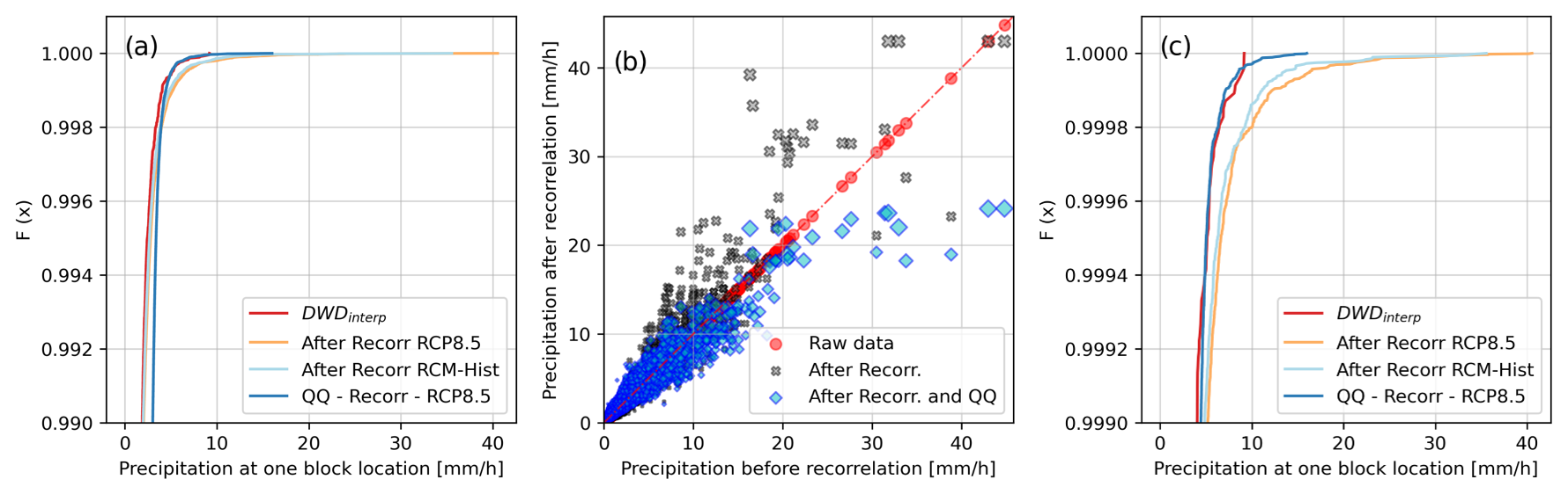
Figure 7 Panel (a) shows the upper 0.5 % of the CDFs of the DWD_interp values (red curve), the EURO-CORDEX historical data (green curve), the recorrelated RCP8.5 data (blue curve), and the double-QQ-corrected RCP8.5 data (black curve). Panel (b) shows the scatter of the values before and after the recorrelation (points in gray) and the double-QQ mapping (points in blue) for one example grid cell location. Panel (c) displays the upper 0.1 % of the CDFs along the Radar_avg values (orange curve).

3.3 Depth–duration–frequency (DDF) curves

To estimate rainfall depth for design values, a statistical analysis of rainfall maxima derived from long records is required. In general, design values are associated with the corresponding duration and return period. The previous concept forms the basis of statistical analysis of heavy rainfall. Rainfall maxima are extracted from the observation time series for different durations by considering either the yearly maxima (annual series) or the values exceeding a minimum threshold (partial series). The relation between rainfall depth, duration, and return period is commonly known as the depth–duration–frequency (DDF) or intensity–duration–frequency (IDF) curve. The idea behind the DDF curve is to derive a mathematical expression relating the average rainfall intensity (i) occurring over a timescale (d) for a predefined return period (T) (Koutsoyiannis and Papalexiou, 2017). DDF curves are used to estimate the probability of non-exceedance of a certain rainfall amount for a given duration. These can be derived by a frequency analysis of the observed station data for different durations. Standard practice is to fit a theoretical extreme value distribution function (e.g., Gumbel type I) to the empirically calculated DDF curve, from which one can derive the possible rainfall depth (or intensity) for a certain return period and timescale. The reasoning behind fitting a distribution function to the sampled annual or partial maxima is that these represent only one realization of the possible rainfall values for the corresponding duration.

In this work, area–depth–duration–frequency (ADDF) curves were derived from the observed annual series of 15 years (2005–2020), following the procedure described by the German Association for Water, Wastewater and Waste in DWA-A 532 (DWA-A, 2012). The extreme value distribution type I, also known as the Gumbel distribution function, is applied in the following form:

$$\begin{array}{}\text{(8)}& h_N\left(T_n\right)=u_j+w_j\left(-\ln \ln {\displaystyle \frac{T_n}{T_n-\mathrm{1}}}\right),\end{array}$$

where h_N represents rainfall depth [mm], T_n represents return period of the annual maxima in years [a], and u_j and w_j represent parameters of the distribution function.

3.4 Area–depth–duration–frequency (ADDF) curves

To calculate precipitation volumes, it is necessary to consider the average precipitation over a given area. Determining ADDF curves is complex because, unlike point precipitation measurements, areal precipitation has to be estimated. Additionally, the spatial patterns and the distribution function of areal precipitation are different from those of point precipitation values.

For example, using weather radar data for a target location of an area of 1000 km², all pixels located within the area are identified, and for every time step the average of all the pixels is calculated. Eventually, a time series is acquired and used as input to the DDF calculation procedure. Bennett et al. (2016) first suggested the use of interpolated rainfall data for the direct estimation of the statistics of areal extremes by introducing the intensity–duration–frequency–area curves. The need for areal reduction factors (ARFs) to convert points to spatial rainfall would then be eliminated. Radar-derived precipitation data can be used to calculate the ADDF curves. However, the quality of the radar reference data and the relatively short observation time period highly influence the results (Haberlandt and Berndt, 2016a). Marra and Morin (2015) used radar quantitative precipitation estimation (QPE) to derive IDF curves for the region of Israel and compared the results to nearby rain gauges. Despite efforts to reduce errors in the radar QPE, the final results showed an increasing overestimation of radar-derived IDF curves for larger durations. Another study by Ghebreyesus and Sharif (2021), using the radar QPE data over the state of Texas (USA) to derive IDF curves, showed mostly an underestimation of short-duration maxima. The goal of using the radar QPE data is to be able to derive spatially and temporally reliable IDF curves, eliminating the need for areal reduction factors (Ghebreyesus and Sharif, 2021).

Areal precipitation extremes derived from weather radar data are prone to errors (Schleiss et al., 2020), e.g., due to attenuation, beam blockage, subscale variability, and simplified Z–R relationships (Villarini and Krajewski, 2010). However, as there is still no possibility to correctly measure areal extremes, the error term cannot be easily quantified. Due to sparse rain gauge networks, many short-duration intense rainfall events cannot be correctly sampled, and many are completely missed (Lengfeld et al., 2020). The high spatial and temporal availability of the RADOLAN gauge-adjusted radar data makes it advantageous for the analysis of areal extremes, and RADOLAN was used in this study for the estimation of reference ADDF curves (DWD Climate Data Center, 2021b). However, due to the limited length of the dataset, the ADDF curves were derived for return periods of 5 years. Such short return periods are relevant for the design of urban drainage networks.

3.5 Downscaling from model to point scales

In order to better assess the quality of the EURO-CORDEX model data when representing areal precipitation extremes, a direct comparison between point observations and model values is not reliable due to scale differences. Therefore, a spatial downscaling of the model grid cell values to a finer scale is required. A deterministic approach, such as an interpolation technique, can only provide one possible subscale realization without any estimate of an uncertainty interval. In general, most interpolation techniques can only provide smoothed fields as, in all kriging applications, the equation system is solved by minimizing the estimation variance. Hence, the interpolated fields have less variability than the original one. However, for hydrological applications, many processes are driven by variability rather than the average values.

To this end, a simulation of many possible realistic realizations with the same dependence structure can offer the corresponding variability. In general, there are two main types of simulation methods: conditional and unconditional simulations. Random mixing is a conditional simulation method that allows for the stochastic generation of realizations that satisfy multiple conditions (Bárdossy and Hörning, 2016). The method is extended from the work of Hu (2000) regarding the gradual deformation of Gaussian fields. In order to achieve the goal of having realistic realizations, the following criteria must be fulfilled by the simulated field:

1. The realizations should match the measured data (conditioned on observations).

2. The realizations should have the same spatial dependence structure (represented by a variogram or spatial copula function).

3. The realizations should have a similar range as the observed values (no extreme values).

The random-mixing methods allow for capturing the spatial dependence structure through a spatial copula function. A copula is a mathematical function used to derive and model the dependence between variables independently of their distribution functions. If a spatial copula function was used, the asymmetry of the spatial field could be better taken into account (asymmetry can be viewed as the measure of skewness of univariate data). Another advantage of random mixing is the possibility to include multiple conditional observations that can be integrated as linear (equality) or nonlinear (inequality) constraints. As a stochastic method, several equally possible realistic realizations of a certain event (or time step) can be derived along the associated mean uncertainty field.

In this work, random mixing was used to upscale and downscale the DWD_point observations to the EURO-CORDEX scale and vice versa using the RMWSPy Python package developed by Hörning and Haese (2021). First, based on the DWD_point data for the period 2005–2020, conditional fields were simulated for every time step with precipitation >1 mm. The simulated fields were conditioned on the DWD_point observations, the corresponding marginal distribution function, and the fitted covariance (or variogram) model representing the spatial dependence structure.

In this step, the calculated experimental variogram was normed and saved. Note that because the variogram was calculated in the rank space, its estimation was smoother than by using the original observations. Eventually, a K-means clustering was applied, and three clusters of variograms were identified (Hartigan and Wong, 1979). Different numbers of clusters were tested, but the chosen number of clusters (three) was found to be the most suitable as the fitted models were the most distinct. For each cluster, the mean variogram was calculated, and an exponential variogram without a nugget was fitted. Since the EURO-CORDEX data are on the grid cell scale, the estimated spatial model is smoother than that of the point scale. Hence, for downscaling, the spatial dependence model calculated from the grid cell values needed to be rescaled to the point scale. To that end, using the EURO-CORDEX data, the experimental variograms were calculated, and a similar clustering approach was applied. This allowed for assigning a suitable variogram for every time step and duration. A similar approach of variogram clustering was presented in Bárdossy et al. (2021).

Figure 8 shows the fitted exponential variograms for each average cluster variogram from the point and model data. The grid cell variograms show a similar behavior as those derived from the point scale but with a smaller variance and a larger range. In other terms, for the same separating distance, the variance of the grid cell model is smaller than that of the point model. The parameters of all average cluster variogram models can be found in Table A1.

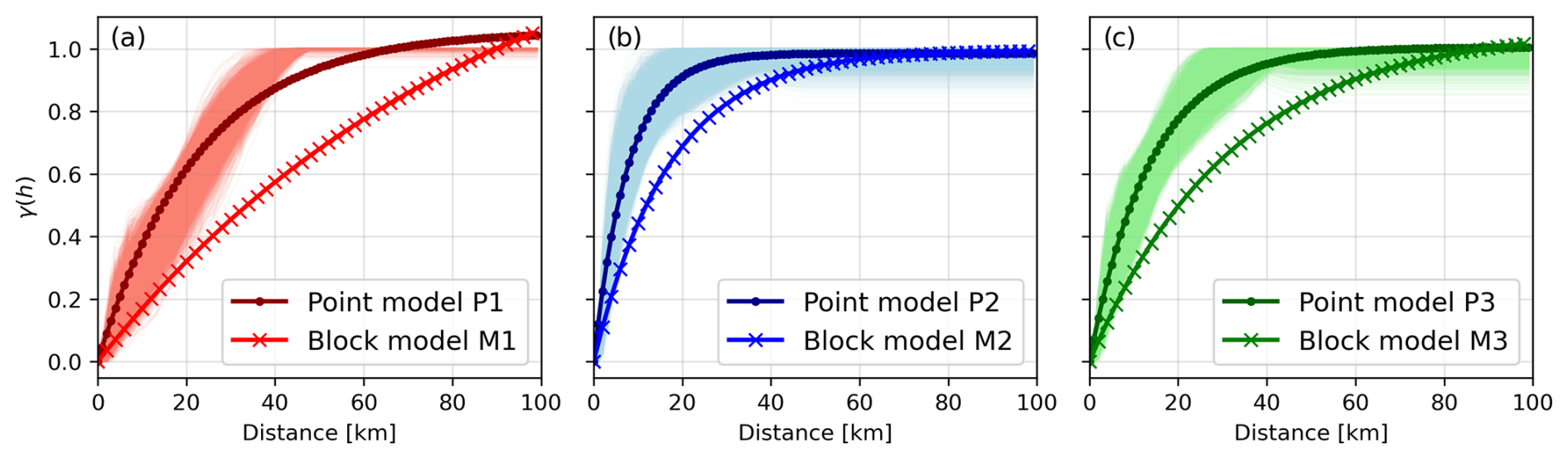
Figure 8 The calculated and clustered hourly experimental variograms using DWD_point are shown in panels (a), (b), and (c). Each panel corresponds to a different variogram cluster. The theoretical models fitted to the average experimental variogram model of each cluster group (using DWD_point) are denoted by point model P1, point model P2, and point model P3. These are displayed by the dark red, dark blue, and dark green curves. Similarly, the fitted theoretical models to the average cluster variogram using EURO-CORDEX RCP8.5 data are denoted by block model M1 (light red curve in panel a), block model M2 (light blue curve in panel b), and block model M3 (light green curve in panel c), respectively.

For each time step in the RCP8.5 data, the corresponding variogram cluster was identified, and the corresponding point scale variogram was used to rescale the spatial model. Without rescaling the grid cell variogram to the point variogram, the downscaled fields would be much smoother than the actual 1 km fields.

Once the spatial dependence structure and the bias in the cumulative distribution function (CDF) of the future RCP data were adjusted, conditional realizations were produced at a finer spatial resolution of 1 km, corresponding to the weather radar grid. This was achieved through a process called random mixing, which constitutes the downscaling phase. It is important to note that this section relates to part (c) in the flowchart shown in Fig. 2. This process incorporates the climate signal from the projections and provides a dataset that can be used to derive future ADDF curves for the study area. To account for the uncertainty acquired by the simulation approach, 50 downscaled and equally probable time series for every pixel in the simulation domain were generated.

The step-by-step procedure to downscale the EURO-CORDEX RCP8.5 data for the period 2005–2099 for a given ADDF location using random mixing is described below:

1. create a buffer enclosing the ADDF largest area (1024 km²);

2. find all EURO-CORDEX grid cells falling within the buffer (conditional values);

3. find all radar pixels falling within the buffer (simulation domain);

4. for every hour in the projected RCP8.5 data with precipitation >1 mm, read corrected values;

5. fit a nonparametric marginal distribution using a kernel density estimate with a Gaussian kernel;

6. derive the CDF and its inverse (invcdf) by optimizing the kernel bandwidth;

7. transform the observations to standard normal space using the fitted CDF;

8. fit an exponential covariance model;

9. scale the model to match the reference point model;

10. run conditional simulations (50 simulations);

11. back-transform to original data space using invcdf;

12. repeat for the next time steps.

An example of the simulation domain for one ADDF location is shown in panel (a) of Fig. 9. The domain shown in red has a total area of 1024 km². Within this domain, the areas of 1, 16, 36, 100, 256, 576, and 1024 km² were considered for deriving the ADDF curves. These are derived as DDF curves using a time series of the average of all pixels within each area. For example, for the area of 1024 km², for every time step the average of the pixels enclosed by this area (pixels in red) was calculated. Using the same procedure for DDF curves (described in Sect. 3.3), the ADDF curve for this area was derived. In panel (a), the gray pixels represent the complete simulation domain, and the blue dots are the center of the EURO-CORDEX grid cells. The precipitation values at these grid cells were used as equality constraints in the downscaling part. To showcase the influence of the variogram scaling procedure, two different spatial dependence models were used: block model M2 (derived from EURO-CORDEX data) and point model P2 (derived from DWD_point). Both models can be seen in panel (b) of Fig. 8. Because the simulations using random mixing are stochastic, it is difficult to compare them; hence, for comparison purposes, the average of 50 simulations was considered. Therefore, 50 realizations were generated using both models, and the average fields were compared. Panels (b) and (c) in Fig. 9 display the average fields using variogram model M2 and variogram model P2, respectively. Note that the main difference in the spatial models is their range and how they approach the asymptotic limit. In panel (b), the larger range in model M2 is reflected by larger connected high (or low) rainfall grid cells and less variability in the final field, noted by the transition between wet (or high) and dry (or low) rainfall areas. The field in panel (c), which is based on model P2, has more variability, and the smaller range is reflected by more discontinuities between the high and low values. Note that both average fields were conditioned on the same recorrelated and double-QQ-corrected RCP8.5 data. Consequently, in order to account for this variation in the subscale downscaled fields, it was necessary to rescale the grid cell variograms to align with the point scale.

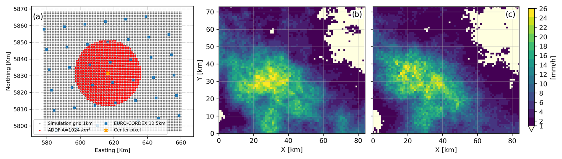
Figure 9 Panel (a) shows the 1 km simulation grid domain (in gray) and the locations of the center of the EURO-CORDEX grid cells (blue dots) within the ADDF (largest area of 1024 km²) (shown in red). Panels (b) and (c) display the average of 50 simulated fields using random mixing based on the RCP8.5 data (the blue dots in panel a), using the original grid cell variogram (model M2) and the rescaled variogram (point P2) respectively. Note that the field in panel (c) depicts larger variability.

4 Results

4.1 ADDF curves for future scenarios

4.1.1 ADDF curves for small spatial scales

The downscaled fields are used to calculate the ADDF for selected regions/pixels in the study area. The aim is to derive areal extremes for future periods, particularly from the RCP8.5 data. The realizations generated by the conditional simulations are all equally probable but limited to spatial constraints and not temporally correlated (e.g., advection is not included). Therefore, for each time step with precipitation >1 mm, 50 simulations were generated across the simulation domain for each duration separately. This was essential; otherwise, the fields would not be space-time continuous. For example, on the hourly scale, each realization for each time step will most likely be different from the realization of the next time step, despite being equally probable and statistically correct. Aggregating these fields will lead to an incorrect representation of the areal rainfall. A simple but computationally intensive solution was to aggregate the hourly corrected data for each required duration and rerun the simulations again. A different possible solution would have been to use the generated fields for time step i as unconditional fields (instead of random fields) for time step i+1. This would have required modifying the simulation algorithm to include time as a third dimension. However, since the focus is on areal statistics, especially annual maxima, and not on event reconstruction, the first solution was seen as adequate enough for this scope. Moreover, an alternative stochastic simulation approach could have been tested. For example, Papalexiou et al. (2021) and Bárdossy and Hörning (2023) present frameworks for simulating space-time rainfall fields with characteristics such as velocity field, advection, anisotropy, and a flexible dependence structure.

After the simulations were completed, the ADDF curves for the area of 1 km² were calculated from the generated time series for four different time periods: 2005–2025, 2026–2045, 2046–2064, and 2065–2099. For comparison purposes, the simulations were performed using the raw data, the double-QQ data, and the recorrected and double-QQ-corrected RCP8.5 data. The ADDF curve from RADOLAN data for the period 2005–2020 was calculated as reference data. Figure 10 shows an example of the ADDF values for the center pixel in the ADDF location (seen in panel (a) of Fig. 9) for the return period of 5 years and for two different time periods: panel (a) for the period 2005–2025 and panel (b) for the period 2065–2099. Each boxplot for every duration consists of 50 simulations. The ADDF values for the different durations from the raw, the double-QQ-corrected, and the double-QQ and recorrelated RCP8.5 data are shown in the blue, orange, and green boxes, respectively. The blue crosses, the orange crosses, and the green dots represent the outliers in the raw and corrected RCP8.5 data, respectively. As reference data, the ADDF curve from RADOLAN data for the period 2005–2020 was calculated and is displayed as the dashed red line (and crosses).

Compared to the RADOLAN data, the raw RCP8.5 values for both periods show an overestimation of the maxima over all durations. The final corrected values (green boxes), however, fall within the range of the RADOLAN data and show a good agreement for the period 2005–2025. Additionally, the boxplots of the raw data indicate a larger range compared to the corrected data. For example, the estimated rainfall depth from raw data for the duration of 720 min (12 h) varies between 40 and 100 mm with a mean value of 60 mm. However, in the corrected data, the range is between 25 and 40 mm. This indicates that the raw data have greater spread and variability, which makes it difficult to use a trustworthy uncertainty interval. Using the double-QQ correction alone improved the results compared to the RCP8.5 raw data, but agreement was still far from the RADOLAN data. This also indicates the need for correction of the spatial dependence structure.

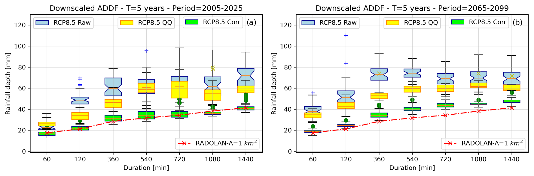
Figure 10 Derived ADDF curves (A=1 km²) from RCP8.5 data before and after data correction for the ADDF center pixel for two different periods and a return period of 5 years. In panel (a) data are for the period 2005–2025, and in panel (b) data are for the period 2065–2099. For every duration (x axis), 50 simulations were generated and summarized in the boxplots. In both panels, the blue boxes refer to the raw RCP8.5 data, the yellow boxes to the double-QQ-corrected data (without recorrelation), and the green boxes to the recorrelated and double-QQ-corrected RCP8.5 data. The rainfall depth values derived from the RADOLAN data for the period 2005–2020 are displayed by the red crosses (or red curve).

In all datasets, an increase in the expected rainfall depth from the first to the second period is clearly visible, although with different magnitudes. Panel (b) of Fig. 10 shows the ADDF for the period 2065–2099 and indicates an increase in the expected rainfall depth for all durations and a return period of 5 years. However, the increase is not homogeneous across all durations and varies accordingly.

4.1.2 ADDF curves for larger spatial scales

From the downscaled fields, the ADDF curves were derived from the raw, the double-QQ, and the recorrelated and double-QQ-corrected fields and compared to the RADOLAN values. The results are displayed in Fig. 11. The purpose of this analysis is to showcase if the pixel (point) and areal extremes show similar behaviors. The results of this approach are shown in panels (a) and (b) of Fig. 11 for the periods of 2005–2025 and 2065–2099, respectively. The ADDF curve for the area of A=1024 km² and return period of 5 years is shown and compared to the RADOLAN values. Compared to the RADOLAN values, the ADDF values from the raw and the double-QQ-corrected data show an overestimation of the ADDF curves for all durations and both periods. Similar results were noted for smaller areas (e.g., 16, 36, 100, 256, and 576 km²). The final corrected data are in agreement with the RADOLAN results and indicate an increase in the areal rainfall depth for all durations in Fig. 11b. Moreover, the raw data (boxes in blue) show a large uncertainty interval. The corrected data indicate, however, a smaller uncertainty interval across all durations. In addition, the uncertainty interval for larger areas is less than for smaller areas. In other words, the single pixel ADDF (1 km²) curve shows the largest variations, while the ADDF curve for A=1024 km² shows the smallest.

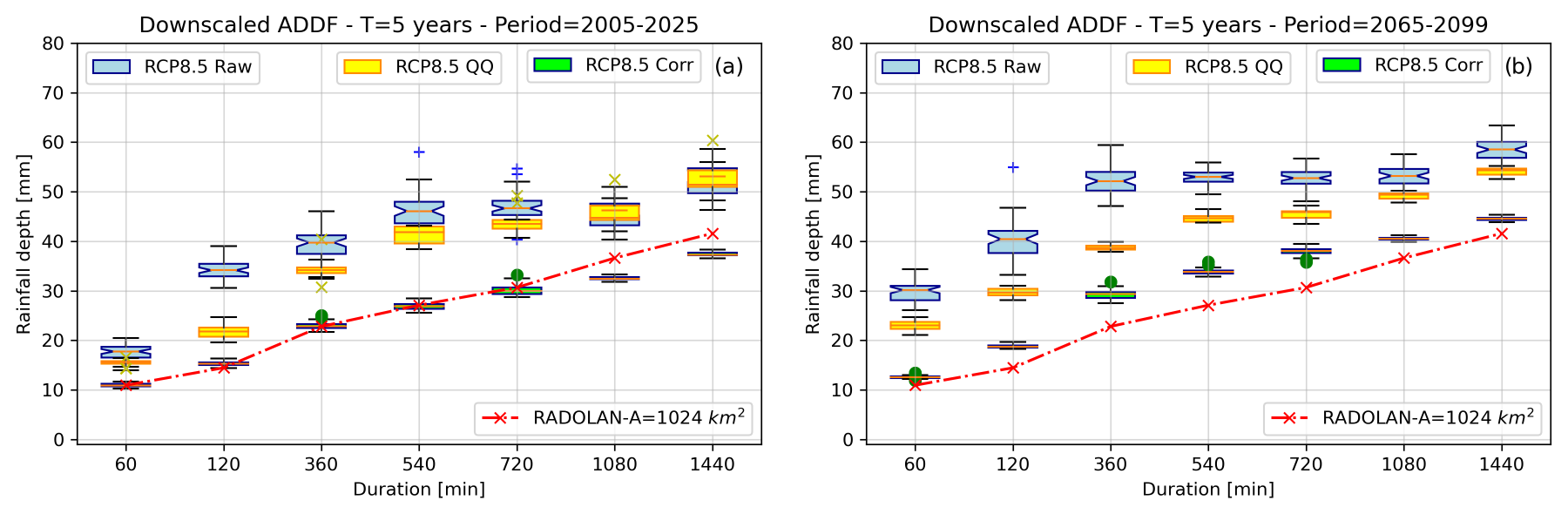
Figure 11 Estimated rainfall depth and ADDF curve from RCP8.5 data before and after data correction for the ADDF area of 1024 km² for a return period of 5 years. For every duration (x axis), 50 simulations were generated and summarized in the boxplots. Panel (a) shows the results for the period 2005–2025. In panel (b), the ADDF curve for the period 2065–2099 is displayed. In both panels, the blue boxes refer to the raw RCP8.5 data, the yellow boxes to the double-QQ-corrected data (without recorrelation), and the green boxes to the recorrelated and double-QQ-corrected RCP8.5 data. The rainfall depth values derived from the RADOLAN data for the period 2005–2020 are displayed by the red crosses (or red curve).

Looking at the variation in the estimated rainfall depth across the different spatial scales (i.e., the ADDF areas), it was found to be dependent on the duration. For instance, the difference in ADDF values between smaller areas (1 or 16 km²) and larger areas (576 or 1024 km²) varies when comparing hourly data to 6-hourly data. In particular, the difference between spatial scales decreases with increasing duration, meaning that over longer durations larger areas tend to respond similarly to smaller ones. To illustrate this, the 1 and 6 h durations were chosen as an example. For the hourly scale, the difference between the average estimated rainfall depth for the small area of 16 km² and the largest area of 1024 km² is around 25 %, while for the 6 h duration the difference is 5 %. Panel (b) of Fig. 13 shows the estimated rainfall depth for two durations for each area separately. The data are derived from the final corrected data and for the time period 2065–2099. The green boxplots show the hourly values, and the orange boxplots show the 18 h values. The RADOLAN values are displayed by the red dots.

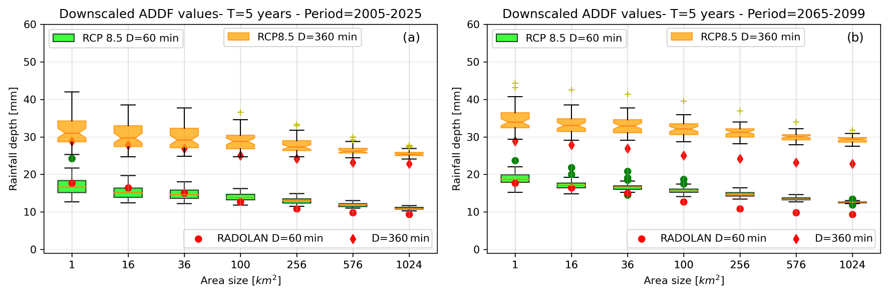
Figure 12 Estimated rainfall depth from RCP8.5 data after data correction for different areas, two selected durations (1 and 6 h), and a return period of 5 years. For every duration, 50 simulations were generated and summarized in the boxplots. Panel (a) shows the results for the period 2005–2025, and panel (b) shows results for the period 2065–2099. The rainfall depth values derived from the RADOLAN data for every duration and for the period 2005–2020 are displayed by the red dots, which are constant for the two time periods.

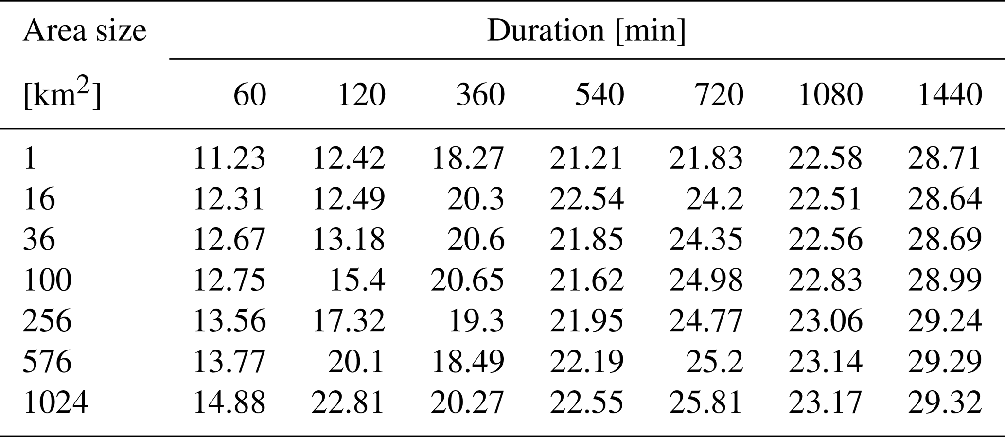
In Table 2, the average percentage of increase in the expected rainfall depth between the two time periods and for the different durations and areas is shown. The percentage was calculated as the ratio between the mean estimated rainfall depth for the two time periods of 2005–2025 and 2065–2099 for the corresponding area and duration. The results in Table 2 indicate that the impact of climate change on the different spatial scales is duration dependent. For instance, on the hourly scale, the percentage of increase is bigger for the larger areas than for the smaller areas, namely, 15 % for the area of 1024 km² and 11 % for the area of 1 km². This difference is minimal for durations longer than 8 h. For instance, on the 18 h duration, all areas have a similar percentage of increase (≈23 %). On the other hand, the percentage of increase changes with the duration for a fixed area. For example, for the area of 100 km², the increase for the hourly duration is 12 %, while for the daily duration it is 28 %. One would expect a monotonic increase with the area and duration. This is mostly the case, but there are some exceptions such as the duration of 6 h when the area of 256 km² shows a slightly larger average increase than the area of 576 km². This indicates that applying a constant increase factor is not adequate and could lead to an incorrect estimation of the future areal extremes.

Table 2 Average percentage of increase in the expected rainfall depth between the periods of 2005–2025 and 2065–2099 for the different durations and areas. The values correspond to the ratio between the average expected rainfall depth value for the two different time periods.

4.2 Areal reduction factor values for future scenarios

A final point to mention is that the ARF values can be calculated as the ratio between larger and smaller ADDF curves. An example of this can be seen in Fig. 13. Panel (a) shows the ARFs calculated as the ratio between the estimated rainfall depth of 1024 and 1 km² areas for the period 2005–2025, using the raw data (blue boxes) and the final corrected data (green boxes). The x axis denotes the duration (from hourly to daily), and the y axis is the ARF value (usually between 0 and 1). The ARFs derived from the RADOLAN values are shown by the red dots. The results in panel (a) indicate that the raw data underestimate the ARFs, especially for longer durations. The corrected data show a better agreement with the RADOLAN data. Note that the ARF is traditionally used to transfer the DDF curves calculated from the point scale (i.e., rain gauge data) to the catchment or areal scales. For instance, the RADOLAN data indicate that for the hourly duration the expected rainfall depth for the area of 1024 km² is 62 % of the center pixel rainfall depth. The corrected data indicate an average ARF of 0.64 (64 %). As the duration increases, the ARF approaches the value of 1, indicating that for a long duration small and large spatial scales behave similarly.

In panel (b) of Fig. 13, the ARF values were calculated using the final corrected RCP8.5 data for two different temporal periods and for a return period of 5 years. For the period 2005–2025, the ARF values are presented by the green boxes. The ARF values for the period 2065–2099 are shown in the gray boxes. The results show that the future period has larger ARF values for short durations and similar values for longer durations. This indicates that the distribution of large-to-small spatial-scale areal rainfall will change for future periods. Specifically, the increase in rainfall depth for the large areas (1024 km²) is greater than that of the smaller scale (1 km²). Similar results were found for other areas.

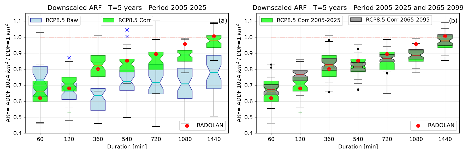
Figure 13 Panel (a) shows the estimated areal reduction factors (ARFs) from RCP8.5 data before and after data correction for a return period of 5 years and the time period of 2005–2025. The results are for the areas of 1 and 1024 km². For every duration (x axis), 50 simulations were generated and summarized in the boxplots. In panel (a), the blue boxes present the ARFs from the raw data, and the green boxes refer to the corrected RCP8.5 data. In panel (b), the ARFs are derived from the corrected data from the time periods of 2005–2025 (green boxes) and of 2065–2099 (gray boxes). The ARF values derived from the RADOLAN data for the period 2005–2020 are displayed by the red dots in both panels.

4.3 Discussion

The final results indicate that the proposed methodology succeeded in obtaining reliable areal extremes from regional climate models over several durations and spatial scales. Using the RCP8.5 data from the model without any correction showed an overestimation of the derived ADDF curves across all temporal durations and considered periods. The overestimation was evident in comparison to the values derived from RADOLAN for the period 2005–2020. The double-QQ method corrected the bias in the marginal distribution function but was not sufficient to achieve values in the range of the RADOLAN data. The recorrelation procedure, namely, the correction of the spatial dependence structure, was needed. To handle the large number of 0 mm values, the recorrelation had to be applied to the Gaussian-transformed indicator correlation time series. This improved not only the pairwise Pearson correlation but also the rank correlation (Spearman correlation). Eventually, the combination of the recorrelation method and the double-QQ transformation was needed. In fact, since the recorrelation procedure is based on indicator correlations, applying it before or after the double-QQ mapping makes no difference. The indicator correlation is not sensitive to quantile mapping. For downscaling to the smaller spatial scale, the corrected data were used as conditional values within a stochastic downscaling algorithm. This gave an uncertainty interval for each ADDF curve. However, as part of the downscaling, the spatial dependence model needed to be rescaled to achieve larger small-scale variability. The final derived ADDF curves were in the same range as the RADOLAN values for the period 2005–2020. The procedure used consisted of many steps but was necessary to obtain reliable results. After the correction and downscaling processes, the signal in the RCP projections remained intact. Increases in areal precipitation values between the initial period (2005–2025) and the final period (2065–2099) were observed both before and after the correction. However, the extent of this increase was less pronounced in the corrected data. The areal reduction factor (ARF) values, derived from the ADDF curves, demonstrated improved alignment with the reference values after correction. These values indicate an increase between the two time periods, particularly for shorter durations, suggesting a shift in the relationship between small- and large-scale precipitation events.

The increase in the expected rainfall depth was obtained for small and large spatial scales (1 to 1024 km²) and for short and long durations. However, this increase was not constant but proportional to the increase in area and duration. For shorter durations, the percentage of increase varied between 10 % and 20 %. For longer durations (above 8 h), the percentage of increase varied between 20 % and 30 %. The results are consistent with other studies that examined the influence of climate change on precipitation extremes. However, the results in this work provide insight into possible future values for areal extremes at various spatial scales (and not just the point scale). Furthermore, the effect of the duration was stronger than the effect of area. If the area is constant, the percentage of increase with the duration is greater than if the duration is constant and the area increases. The largest increase occurs for the daily duration and largest area. Nevertheless, these results are only valid for the specific RCM used in this study and might differ for different models. Using a large number of different climate model outputs with the same chain of methods can show the uncertainty of the results with regard to the input uncertainty. In addition, the Radar_avg data used as current reference are available for the period 2005–2020. As more and longer spatially distributed rainfall data will become available in the future, longer periods for comparison with future scenarios will establish a better foundation since a broader range of climate variability and trends would be included.

The analysis of future areal extremes is essential for adaptation strategies. For practical purposes, such as the design of urban drainage systems, rainfall depth values associated with relatively short return periods of 5 years are required. Moreover, the uncertainty interval obtained from the downscaling scheme provides an ensemble of values needed for risk analysis. The ADDF curves were derived using the DWA-A 532 procedure with the Gumbel distribution. However, there are alternative ways to calculate the DDF curves, e.g., by Koutsoyiannis et al. (1998) or Fischer and Schumann (2018). Subsequently, derived ADDF values will change, and the corresponding results may change as well. Furthermore, the results shown in this work are only valid for relatively small areas (mesoscale catchment size) of up to 1000 km². For larger areas, the areal mean precipitation is less of interest, while the areal distribution becomes more relevant. The correlation structure was presumed to be homogeneous and invariant over time. In other words, the spatial dependence structure is considered to be unaffected by climate change. An aspect that is already present in the raw EURO-CORDEX data (see Fig. A1). This assumption may not be valid. However, the presented approach using the indicator correlation is more robust, although it assumes a multi-normal dependence structure, which may not always be valid. The final results show close agreement with the reference RADOLAN values, although the latter may underestimate the areal extremes.

5 Conclusion

Investigating the changes in the statistical properties of climatic variables, such as rainfall, due to a changing climate, is essential for coping and preparing for future periods. Regional climate models provide useful information about climatic data for historical and future scenarios. These have been generated based on increasing emission levels and, hence, changing the physical, energetic, and thermodynamic balance between the atmospheric components. The outcome of RCM data is, in general, too coarse for local analysis, and often spatial and/or temporal downscaling is applied. For having reasonably downscaled values, the original RCM data should be inspected and eventually corrected. Here, two major aspects are crucial. The first is related to the spatial dependence structure. This influences the distribution of areal rainfall, and a false structure alters any subsequent results. The second is related to the presence of a bias in the data of future periods. A bias in any direction (overestimation/underestimation) of the marginal distribution function affects the temporal structure and the quality of the data. If the model distribution differs largely from the observed one, it would be as if it were not a realization of the same process. Hence, the first and second parts of this paper are related to correcting the spatial dependence structure and the marginal distribution function, respectively. Both of these steps were undertaken on the same spatial and temporal scale as the model data. This required upscaling of the reference data to the model scale. The corrected data can now be integrated into a downscaling scheme. In this part, a probabilistic scheme involving conditional simulations using random mixing was applied. For each time step and duration, several realizations on the 1 km scale were generated and used for analyzing areal extremes. The spatial dependence model derived from the grid cell scale was rescaled to the point scale to have higher variability in the simulated fields. From the final fields, ADDF curves along with ARF values were derived for different temporal periods and spatial scales and compared to the RADOLAN values. The results indicate a good agreement with the RADOLAN values for the current period (2005–2025) and showcase an increase in the areal extremes over all durations and temporal scales for the period 2065–2099. The final results show plausible ADDF curves and ARF values that can be used for impact analysis.

The key findings of this study are as follows:

1. Using regional climate model data directly leads to an overestimation of the areal extremes.

2. Correcting the spatial dependence structure and the magnitudes of the data improves the usability of the data.

3. Spatial downscaling using random mixing is possible and offers uncertainty intervals.

4. The signal in the RCP is not lost and is present in the future areal extremes.

5. The corrected data of the RCP8.5 scenario indicate an increase in the rainfall depth over all temporal and spatial scales.

The study could be further extended and applied to several GCM–RCM products. This will provide an ensemble of possible uncertainty scenarios for future projections of DDF and ADDF curves. Although the procedure would be similar for the different GCM–RCM combinations, the results might differ. The applied bias correction technique could be replaced by a different approach that handles nonlinear relations and outliers in a different manner. For instance, the work of Yoshikane and Yoshimura (2022) presents a bias correction technique using machine learning (a support vector machine regression model) for the correction of hourly precipitation values. In addition, recent advancement in generating high-resolution convection-permitting models (CPMs) provides a better estimate of local extreme precipitation than the RCMs. Fosser et al. (2024) found that using data from the CPM ensemble generated using the CORDEX-FPS Convection project reduced the estimation uncertainty of summer precipitation extremes by more than 50 %. Future work using data from the CPM ensemble is possible; however, this would involve engaging in partnerships with computational resources to assist with reducing the substantial expenses associated with computation. The procedure could be further evaluated for a larger geographical range to encompass multiple regions with diverse climatic conditions. This would facilitate comprehension of regional disparities and enhance the applicability of the results. Moreover, instead of working with ADDF areas, a selected hydrological catchment can also be considered. The resulting future areal precipitation extremes could be integrated into a hydrological model to assess the impact on the discharge values and establish practical impact studies regarding flood risk assessments and water resource management.

Appendix A: Additional figures

A1 Rank correlation values for the EURO-CORDEX historical and future data

Figure A1 shows the pairwise grid cell rank correlation values for the EURO-CORDEX historical and future data. Panel (a) shows the results for the winter period, and panel (b) shows them for the summer period. In addition, the correlation values were calculated for the pixels falling within the same direction as compared to the center of the study area. This had no effect on the relation between the correlation values of the two datasets. Hence, the agreement between the historical and future correlation values is very high and indicates a stable dependence structure between the two periods.

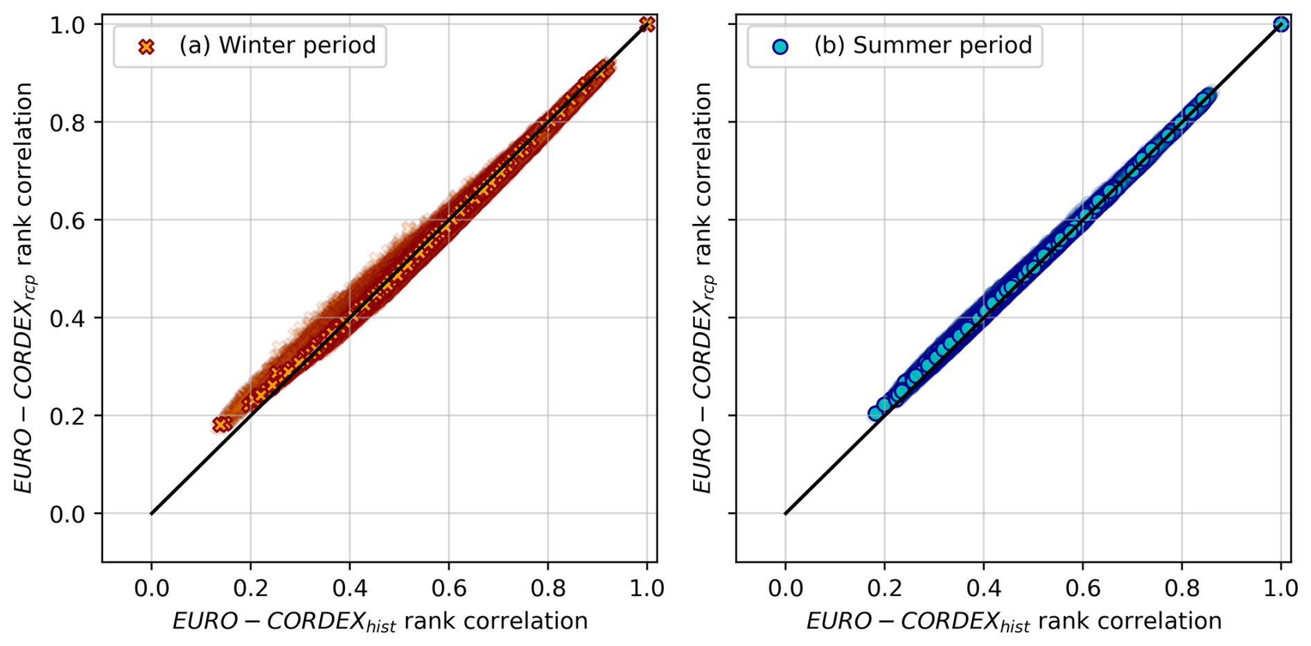
Figure A1 Scatterplot for the rank correlation values between historical and future (RCP) EURO-CORDEX data for winter (a) and summer (b) periods.

A2 Relation between the indicator and Gaussian correlation values

Figure A2 presents the relation between the indicator and Gaussian correlation values for different thresholds α. Note that the curves are only shown for the positive correlation domain [0, 1]. Each curve is obtained by solving the relation defined in Eq. (4) for the corresponding α.

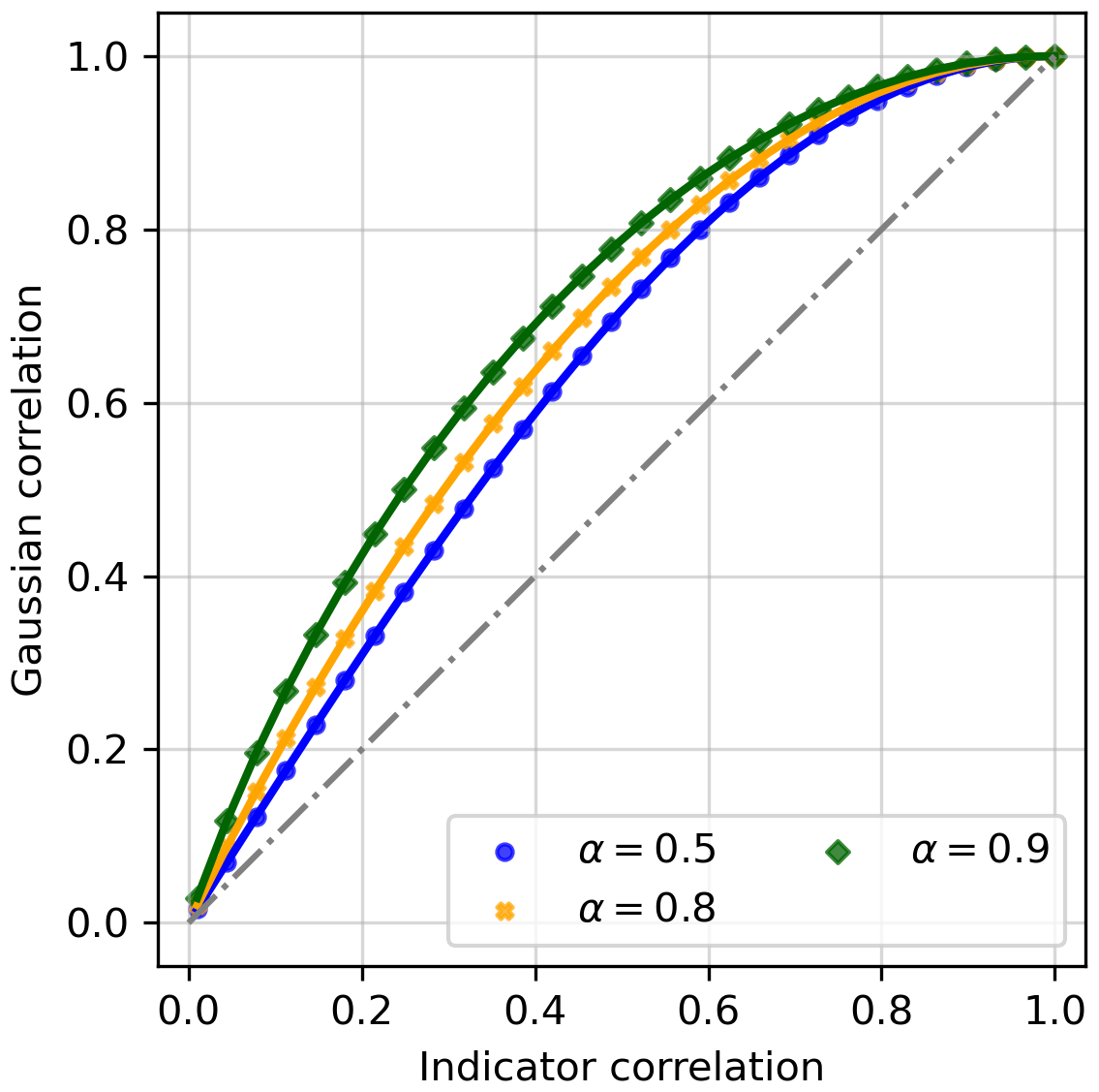
Figure A2 The relation between the indicator and Gaussian correlation used to transform the indicator correlation matrices to Gaussian correlation matrices. Each curve corresponds to a different probability level α. Note that only positive correlation values are shown.

A3 Theoretical variograms parameters

Table A1 shows the estimated parameters of the three theoretical exponential variogram models. These were fitted to the average empirical variogram of every cluster (shown in Fig. 8) using the DWD_point and the EURO-CORDEX data.

Table A1 Parameters of the fitted experimental variograms using DWD_point and the EURO-CORDEX grid cell data.

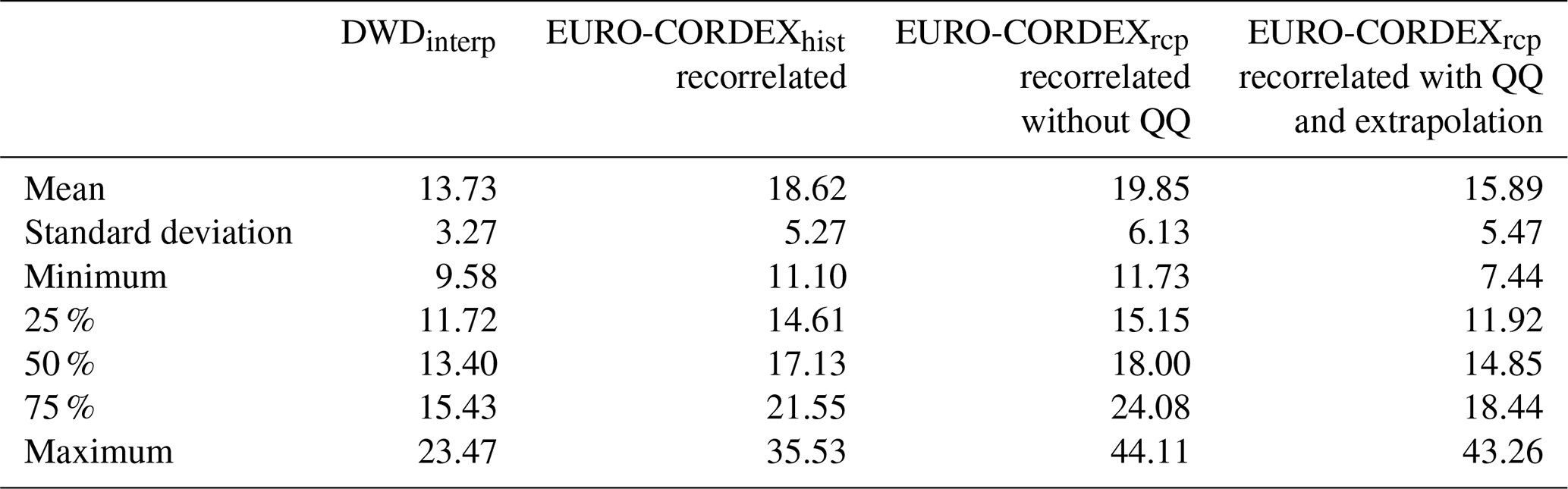
Table A2 Summary statistics for hourly precipitation values [mm h⁻¹] for U>U_m. The descriptive statistics are derived from 322 values.

A4 Effect of extrapolation

The aim of this section is to display the effect of the extrapolation within the double-QQ mapping. The extrapolation procedure is only applied to the values in the recorrelated EURO-CORDEX_rcp data exceeding the maximum observed DWD_interp precipitation values (Z>Z_m; namely, for U>U_m) at the corresponding grid cell location. The parameter λ is calculated from Eq. (7) for every location separately using the pair of the largest precipitation observation and corresponding probability level (Z_m,U_m). Table A2 showcases summary statistics for the EURO-CORDEX_rcp hourly values exceeding the maximum DWD_interp. These were gathered from all grid cell locations (in total 322 values). The first column, DWD_interp, displays the statistics of the maximum values as observed within the DWD_interp dataset. If no extrapolation were performed, i.e., assuming that the rain gauge network observed all maximum rainfall values correctly, the upper bound of the double-QQ procedure would be these values. In other words, all EURO-CORDEX_rcp data would not exceed the values in column DWD_interp. The second column displays the values for the recorrelated EURO-CORDEX_hist for the same indices (where Z>Z_m in EURO-CORDEX_rcp). These values are presented here for comparison purposes. The third column displays the values after recorrelation and before the double-QQ mapping. Following the procedure described in Sect. 3.2, for every Z>Z_m in EURO-CORDEX_rcp, the corresponding quantile U is identified, and using the inverse of Eq. (6), $Z^{*}=-\ln (\mathrm{1}-U)/\mathit{\lambda }$ is estimated. In the case where the value is very large, exceeds the maximum of DWD_interp and EURO-CORDEX_hist, and shows unrealistic values, Eq. (A1) was applied. The latter restricts the extrapolation by a linear component following the procedure described in Yan et al. (2020). However, this was rarely applied, as the recorrelation procedure reduced the impact of very large values. The last column of Table A2 represents the statistics of the Z^* values after the extrapolation and the double-QQ mapping. This displays the effect of the extrapolation and provides values larger than DWD_interp but within the range of the recorrelated EURO-CORDEX_hist.

$$\begin{array}{}\text{(A1)}& F\left(z\right)=min\left(\mathrm{1}-e^{-\mathit{\lambda }z},{\displaystyle \frac{U_m-U_{m-\mathrm{1}}}{Z_m-Z_{m-\mathrm{1}}}}+U_m\right),\end{array}$$

with (Z_m, U_m) and (Z_m−1, U_m−1) defining the pairs of the two largest precipitation observations and corresponding probability levels.