Learning from a large-scale calibration effort of multiple lake temperature models

Process-based lake temperature models, formulated on hydrodynamic principles, are commonly used to simulate water temperature, enabling one to test different scenarios and draw conclusions about possible water quality developments or changes in important ecological processes such as greenhouse gas emissions. Even though there are several models available, a systematic comparison regarding their performance is currently missing. In this study, we calibrated four different one-dimensional (1D) lake temperature models for a global dataset of 73 lakes to compare their performance with respect to reproducing water temperature, and we estimated parameter sensitivity for the calibrated parameters. The parameter values, model performance, and parameter sensitivity differed between lake models and between clusters that were defined based on lake characteristics. No single model performed best, with each model performing better than the others in at least some of the lakes. From the findings, we advocate the application of model ensembles. Nonetheless, we also highlight the need to further improve weather forcing data, individual models, and multi-model ensemble techniques.

1 Introduction

The global rise in water temperatures in lakes and reservoirs (O'Reilly et al., 2015; Pilla et al., 2020) is affecting water quality and ecosystem services worldwide in multiple ways, e.g., by promoting the formation of harmful cyanobacteria blooms (Huisman et al., 2018), modifying lake ice phenology (Knoll et al., 2019), affecting ecosystem functioning (Kattel, 2022), or increasing deep-water oxygen depletion (Jane et al., 2023). Water temperature is a “master variable” in aquatic biogeochemical cycling, involved in processes including the kinetics of metabolism (Staehr et al., 2010) and greenhouse gas emissions (Audet et al., 2017). Moreover, the vertical temperature structure controls mixing rates between water layers and modifies the position of organisms in the water column as well as the light and nutrient conditions that they experience. As such, global future estimates of various water quality and ecological processes in inland waters should be based on an accurate model representation of the present and future conditions of lakes' temperatures and thermal structures that addresses the variability in lake characteristics worldwide. Recent continental- and global-scale modeling efforts have presented convincing evidence of the large impact of climate warming on lake temperatures (e.g., Woolway et al., 2021b; Golub et al., 2022). However, lake models can only be calibrated for comparatively few lakes for which in situ, depth-resolved observations exist. Furthermore, there is a knowledge gap on how model performance is affected by different lake-specific characteristics and how models could be parameterized based on the lake characteristics when applied on a global scale. At the moment, it is common in global lake modeling studies to apply models without lake- or region-specific calibration (e.g., Woolway et al., 2021a; Vanderkelen et al., 2020), and this adds considerable uncertainty to projections of climate change impacts on lake water temperatures.

Vertical one-dimensional (1D) lake models, based on hydrodynamic principles, are efficient tools to simulate water temperature dynamics for lakes in which the vertical density gradient is more pronounced than the horizontal one. Piccolroaz et al. (2024) gave an extensive review of the theoretical considerations for water temperature modeling across different spatial dimensions and noted the frequent use of 1D models in climate simulations due to their low computational costs and adequate performance. Previous studies have indicated that optimal model parameter values may depend on certain lake characteristics, which could help to obtain more accurate fits in global applications. For instance, an application of the 1D physical lake model GLM (General Lake Model; see Hipsey et al., 2019) with a sensitivity analysis of nine model parameters across multiple lakes suggested that the sensitivity of a subset of parameters depended on characteristics such as lake depth, water transparency, and residence time (Bruce et al., 2018). In a multi-lake application of the 1D physical model ALBM, Guo et al. (2021) highlighted the relationships between the relative influence of model parameters and lake characteristics such as latitude and lake depth. Extending beyond physical variables, Andersen et al. (2021) performed an extensive, global sensitivity analysis on the 1D coupled physical–biogeochemical model GOTM-FABM-PCLake in three Danish lakes and found that parameter sensitivity may be strongly linked to lake morphology in shallow lakes, including a potential feedback of biogeochemical components on temperature (such as light absorption by organic matter).

In this study, we applied four 1D physical lake models to a set of 73 lakes for which in situ water temperature observations were available, as part of the Inter-Sectoral Impact Model Intercomparison Project (ISIMIP; Golub et al., 2022), using meteorological forcing from bias-corrected reanalysis data. The models were calibrated in a consistent manner, and we report on the overall model performance, highlight consistent patterns in model performance and parameter values, and the assessed parameter sensitivity. These calibrations were in preparation for ISIMIP climate impact simulations for the local lakes sector (see the Code and data availability statement). This study approach expands on previous studies through testing the sensitivity of multiple models simultaneously by applying an identical methodology for calibration and sensitivity analysis implemented over a larger number of lakes. Such an in-depth model evaluation on a global scale can accomplish the following:

1. point towards systematic issues and biases in 1D physical lake models when forced by meteorological reanalysis data;

2. reveal patterns in model performance driven by geographic location and/or lake characteristics;

3. test if an optimal model for specific lake types exists, or alternatively, advocate for an ensemble approach;

4. identify a set of highly sensitive parameters for calibration.

This will expand our knowledge of the accuracy of water temperature modeling on a global scale; improve our understanding of the relationship between lake characteristics and model parameterization, thereby providing practitioners with advice on how to best calibrate certain lake types; and, potentially, lead to more accurate model application. As there is a growing interest in global estimates of water quality and greenhouse gas emissions (e.g., Kakouei et al., 2021; Jansen et al., 2022; Jane et al., 2023; Zhuang et al., 2023), which often rely partially on simulated water temperature and thermal structure, we need to ensure that the underlying global thermal information is as accurate as possible and that the level of uncertainty is known.

2 Methods

2.1 ISIMIP local lakes

ISIMIP – the Inter-Sectoral Impact Model Intercomparison Project – is a framework for consistently projecting the impacts of climate change across affected sectors and spatial scales (https://www.isimip.org/, last access: 20 February 2025; Frieler et al., 2024). The ISIMIP Lake Sector considers the impact of global warming on two categories of lakes: “local lakes” and “global lakes” (Golub et al., 2022). The local lakes were used for this study: 73 lakes for which observed in situ water temperature data and hypsographic information are available (Table S1 in the Supplement). The resolution (vertical and temporal) of the observed data and the detail of the hypsograph varied for each lake. For all but two lakes, data covered a period of at least 1 year; for 75 % of the cases, they covered at least 5 years. Profiles (three unique depths or more) were provided for all but four lakes, and all lakes had more than 100 unique observations (Fig. S1 in the Supplement). A link to the observed data and hypsographs is provided in the Code and data availability statement. No inflow or outflow data are available, so we assumed a constant water level throughout the simulation.

For the forcing of the models, we used the GSWP3-W5E5 reanalysis dataset, which combines the GSWP (Kim, 2017; Dirmeyer et al., 2006) and the W5E5 datasets (Lange et al., 2021; Cucchi et al., 2020). The meteorological forcing, available at daily resolution, for each lake was extracted by the ISIMIP organizational team for the grid cells (at a spatial resolution of 0.5° × 0.5°) in which each lake was located (Golub et al., 2022). The following meteorological variables were used to drive the lake simulations: air temperature, relative humidity, precipitation, shortwave radiation, longwave radiation, surface air pressure, and wind speed.

Initial conditions were estimated from observed water temperatures. Therefore, all available data in a period of days (depending on data availability) before and after the start date of the simulation were taken and averaged to set the initial temperature profile. All simulations used a spin-up period of 1 year.

2.2 Lake clustering

In order to analyze the impact of lake characteristics (Table S2) on the model performance and parameter sensitivity, we used K-means clustering to group the 73 lakes (Fig. 1). Prior to clustering, we log-transformed the elevation, mean depth, maximum depth, and lake area and then applied a z-score transformation. We created a silhouette plot to determine the optimal number of clusters, which was two. However, we decided to use five clusters instead, as this gave a more meaningful representation of different lake types (Fig. S2).

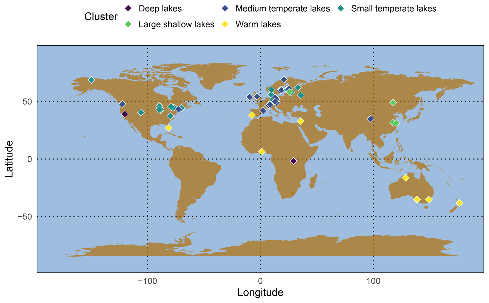
Figure 1 Map showing the locations and grouping derived by K-means clustering of the 73 lakes included in the study.

2.3 The 1D physical lake models

In this study, four vertical lake temperature models with varying algorithms and calculations regarding vertical temperature and heat transport were used to explore the model sensitivity around climate change projections in lakes: the two-layer (0.5D) model FLake (Mironov, 2008, 2005), the 1D integral energy model GLM version 3.1.0 (Hipsey et al., 2019), and the 1D turbulence-based models GOTM lake-branch version 5.4.0 (Burchard et al., 1999; Umlauf et al., 2005) and Simstrat version 2.4.1 (Goudsmit et al., 2002; Gaudard et al., 2019). The models were set up and run using the LakeEnsemblR R package (Moore et al., 2021) to standardize the approach. We refer to Piccolroaz et al. (2024) for detailed information regarding general concepts in water temperature modeling. In this section, we provide a summarized overview of the main differences in process description between these four models. The models were applied in an identical way, with the exceptions that FLake was used to simulate up to the mean depth instead of the maximum depth (in line with assumptions in the model) and that cloud cover was calculated from the meteorological variables using the LakeEnsemblR functions for the GOTM model.

The vertical 0.5D (i.e., a box model but with two separate boxes for upper and lower water layers) lake model FLake was originally designed for weather prediction studies, in which a large-scale climate model is coupled to multiple small-scale lake models. To achieve computational efficiency, FLake simulates the temperature dynamics of an upper completely mixed layer and a thermocline layer (commonly also known as metalimnion), while neglecting temperature dynamics below the latter layer (Mironov, 2005). The vertical temperature evolution itself is parameterized based on the self-similarity concept of the vertical temperature profile (Kitaigorodskii and Miropolsky, 1970). This observed and theoretically explained concept states that a dimensionless temperature profile in the thermocline can be replicated using a “universal” function of the dimensionless depth ζ:

$$\begin{array}{}\text{(1)}& {\displaystyle \frac{{\mathit{\theta }}_s\left(t\right)-\mathit{\theta }(z,t)}{\mathrm{\Delta }\mathit{\theta }\left(t\right)}}={\mathrm{\Phi }}_{\mathit{\theta }\left(\mathit{\zeta }\right)},\end{array}$$

where t and z are the dimensions over time and depth, respectively. In Eq. (1), θ_s is the absolute temperature of the upper completely mixed layer, Δθ(t) is the absolute temperature gradient across the thermocline layer, and Φ_θ is the universal function of the dimensionless depth. The dimensionless depth can be parameterized as follows:

$$\begin{array}{}\text{(2)}& \mathit{\zeta }={\displaystyle \frac{z-h\left(t\right)}{\mathrm{\Delta }h\left(t\right)}},\end{array}$$

where h(t) is the depth of the upper completely mixed layer and Δh(t) is the depth difference between the mixed-layer depth and the bottom of the metalimnion. Note that, in this study, we set the bottom metalimnion depth to each lake's mean depth. Applying this concept to temperature evolution, FLake parameterizes both layers (upper completely mixed and thermocline layer) as follows:

$$\begin{array}{}\text{(3)}& \mathrm{\Theta }=\left\{\begin{array}{lcl}{\mathit{\theta }}_s,& \text{if}& \mathrm{0}<z<h\\ {\mathit{\theta }}_s-\left({\mathit{\theta }}_s-{\mathit{\theta }}_{\mathrm{b}}\right)\mathrm{\Phi }\left(\mathit{\zeta }\right),& \text{if}& h\le z\le D_{\mathrm{lake}}\end{array}\right.,\end{array}$$

where D_lake is the maximum depth (Mironov, 2005). Similar to the other models, the upper completely mixed layer receives the energy fluxes from the atmosphere:

$$\begin{array}{}\text{(4)}& h{\displaystyle \frac{\mathrm{d}{\mathit{\theta }}_s}{\mathrm{d}t}}={\displaystyle \frac{\mathrm{1}}{{\mathit{\rho }}_{\mathrm{w}}{c}_{\mathrm{w}}}}\left(Q_{\mathrm{s}}+I_{\mathrm{s}}-Q_{\mathrm{h}}-I\left(h\right)\right),\end{array}$$

where ρ_w is water density, c_w is heat capacity, Q_s is the turbulent heat flux at the surface, I_s is the surface shortwave radiative flux, Q_h is the heat flux from the bottom to the upper layer, and I(h) is the radiative shortwave flux through the water column (Mironov, 2005). We can state the sum of these individual heat fluxes as the net heat flux exchange (H_net). Although FLake's numerical implementation combines empirical formulations with physical processes, it has demonstrated good performance for surface water temperature modeling as well as ice phenology investigations (e.g., Mallard et al., 2014) and is commonly applied to global studies (Woolway and Merchant, 2019).

GLM, GOTM, and Simstrat are vertical 1D lake models in which temperature evolution is quantified at every time step over a vertical grid. Conceptually, the models differ regarding how the vertical grid is configured: GLM applies a flexible structure, whereas the others use a fixed grid with the possibility of refinements. Nonetheless, all three models are based on the vertical water temperature equation, which – in its general form – can be stated as follows:

$$\begin{array}{}\text{(5)}& {\displaystyle \frac{\partial T}{\partial t}}=\underset{\left(\mathrm{1}\right)}{\underbrace{-{\displaystyle \frac{\mathrm{1}}{\mathit{\rho }{c}_p}}{\displaystyle \frac{\partial I}{\partial z}}}}+\underset{\left(\mathrm{2}\right)}{\underbrace{{\displaystyle \frac{H_{\mathrm{sed}}}{A\mathit{\rho }{c}_p}}{\displaystyle \frac{\partial A}{\partial z}}}}+\underset{\left(\mathrm{3}\right)}{\underbrace{{\displaystyle \frac{S_T}{\mathit{\rho }{c}_p}}}}+\underset{\left(\mathrm{4}\right)}{\underbrace{{\displaystyle \frac{\mathrm{1}}{A}}{\displaystyle \frac{\partial }{\partial z}}\left(A{D}_z^T{\displaystyle \frac{\partial T}{\partial z}}\right)}}.\end{array}$$

Here, the change in temperature T over time depends on four terms on the right-hand side: (1) the internal heat generation due to shortwave solar radiation I, (2) a geothermal heat flux H_sed that acts over an area A, (3) an internal heat source term S_T, and (4) a turbulent diffusive term that includes the eddy-diffusivity coefficient $D_z^T$ (Piccolroaz et al., 2024). The layer adjacent to the atmosphere–water interface receives a net heat flux exchange similar to the one described in Eq. (4), where H_net is the sum of radiative and turbulent heat fluxes:

$$\begin{array}{}\text{(6)}& {\mathit{\rho }}_{\mathrm{w}}{c}_p\left(D_z^T{\displaystyle \frac{\partial T_z}{\partial z}}\right){|}_{z=s}=H_{\mathrm{net}}.\end{array}$$

Here, T_z is the water temperature of the layer adjacent to the atmosphere–water interface at the surface depth s.

The main difference between GLM and both GOTM and Simstrat is how they simulate the turbulent diffusive transport. GLM applies a combination of empirical and physical relationships that use the available external turbulent kinetic energy (TKE) to calculate the thickness of a completely mixed surface layer (for general information about integral energy models, see Ford and Stefan, 1980). For this, mixing in a surface mixed layer is calculated by comparing the available external energy to the potential energy of the water column that is needed to lift up denser water from below a completely mixed layer into a newly formed mixed layer until the TKE is no longer sufficient for further mixing (Hipsey et al., 2019). Below the depth of this surface mixed layer, a parameterization for the eddy-diffusivity coefficient in relation to water column stability is used to calculate diffusive transport:

$$\begin{array}{}\text{(7)}& D_z^T={\displaystyle \frac{C_{\mathrm{HYP}}{\mathit{\epsilon }}_{\mathrm{TKE}}}{N^{\mathrm{2}}+\mathrm{0.6}{k}_{\mathrm{TKE}}^{\mathrm{2}}{u}_{*}^{\mathrm{2}}}},\end{array}$$

where C_HYP is a constant coefficient for the mixing efficiency (later referred to as the calibration parameter coef_mix_hyp), ε_TKE is a simplified approximation of the turbulent dissipation rate based on the dissipation by inflows and wind, N² is the squared buoyancy frequency, k_TKE is the turbulence wave number, and u_* is the wind shear velocity (Weinstock, 1981). The buoyancy frequency (Brunt–Väisälä frequency) quantifies local stability to vertical displacements as follows:

$$\begin{array}{}\text{(8)}& N=\sqrt{{\displaystyle \frac{g}{\mathit{\rho }}}{\displaystyle \frac{\partial \mathit{\rho }}{\partial z}}},\end{array}$$

where g is gravitational acceleration.

Simstrat and GOTM are turbulence-based models that apply a two-equation turbulence model to compute the quantities of the production, transport, and dissipation rates of TKE. Here, we highlight the k−ε two-equation turbulence model which is implemented in both models (Burchard et al., 1999; Goudsmit et al., 2002):

$$\begin{array}{}\text{(9)}& {\displaystyle \frac{\partial k}{\partial t}}={\displaystyle \frac{\mathrm{1}}{A}}{\displaystyle \frac{\partial }{\partial z}}\left(A{D}_z^k{\displaystyle \frac{\partial k}{\partial z}}\right)+P+B-\mathit{\epsilon },\text{(10)}& {\displaystyle \frac{\partial \mathit{\epsilon }}{\partial t}}={\displaystyle \frac{\mathrm{1}}{A}}{\displaystyle \frac{\partial }{\partial z}}\left(A{D}_z^{\mathit{\epsilon }}{\displaystyle \frac{\partial \mathit{\epsilon }}{\partial z}}\right)+{\displaystyle \frac{\mathit{\epsilon }}{k}}\left(c_{\mathit{\epsilon },\mathrm{1}}P+c_{\mathit{\epsilon },\mathrm{3}}B-c_{\mathit{\epsilon },\mathrm{2}}\mathit{\epsilon }\right),\end{array}$$

where $D_z^k$ and $D_z^{\mathit{\epsilon }}$ are the turbulent diffusivities of TKE and TKE dissipation, respectively; P is the TKE production due to shear; and B is the production and dissipation of TKE related to buoyancy (Rodi, 1984). c_ε,1, c_ε,2, and c_ε,3 are empirical constants. In GOTM, whenever the simulated TKE is lower than the calibration parameter k_min , it is set to the value of k_min. We can compute the eddy-diffusivity coefficient $D_z^T$ as a function of the turbulence kinetic energy k and the dissipation rate ε:

$$\begin{array}{}\text{(11)}& D_z^T={\displaystyle \frac{c_{\mathit{\mu }}}{{\mathit{\sigma }}_{\mathrm{t}}}}{\displaystyle \frac{k^{\mathrm{2}}}{\mathit{\epsilon }}},\end{array}$$

where c_μ is an empirical coefficient and σ_t is the turbulent Prandtl number.

Simstrat further employs an empirical seiche excitation and damping model to improve the representation of internal seiches in transport processes (Goudsmit et al., 2002). Here, seiche movement can produce additional TKE, E_seiche, inside the water column with the intention to provide a more realistic simulation of vertical transport due to bottom boundary mixing as seiche motion damping acts as an energy source below the mixed layer:

$$\begin{array}{}\text{(12)}& \begin{array}{rl}{\displaystyle \frac{\mathrm{d}{E}_{\mathrm{seiche}}}{\mathrm{d}t}}& =\underset{\mathrm{PW}}{\underbrace{\mathit{\alpha }{A}_{\mathrm{0}}{\mathit{\rho }}_{\mathrm{air}}{c}_{\mathrm{10}}{\left(u_{\mathrm{10}}^{\mathrm{2}}+v_{\mathrm{10}}^{\mathrm{2}}\right)}^{\mathrm{3}/\mathrm{2}}}}\\ & -\underset{\mathrm{LS}}{\underbrace{C_{\mathrm{Deff}}{A}_{\mathrm{0}}{V}^{-\mathrm{3}/\mathrm{2}}{\mathit{\rho }}_{\mathrm{0}}^{-\mathrm{1}/\mathrm{2}}{E}_{\mathrm{seiche}}^{\mathrm{3}/\mathrm{2}}}},\end{array}\end{array}$$

where PW is energy production, LS is energy loss, α is a model parameter to describe the wind energy fraction that is transferred to the seiche motion (later referred to as the calibration parameter a_seiche), c₁₀ is the drag coefficient, u₁₀ and v₁₀ are velocity components of wind speed measured at 10 m above water surface, and C_Deff is the effective bottom friction coefficient (Goudsmit et al., 2002). We note that similar algorithms, designed to improve vertical mixing dynamics below the epilimnion, also exist in other models, including integral energy models, i.e., the turbulent benthic boundary layer mixing algorithm by Yeates and Imberger (2003), but are not – to the best of our knowledge – implemented in GLM and GOTM.

An additional structural difference between the models is their process description of the treatment of the attenuation of shortwave radiation, especially the nonvisible near-infrared light (NIR) and the visible parts of shortwave radiation. FLake does not distinguish between these parts of the light spectrum, and it applies the Beer–Lambert law for light attenuation with depth (see also Stepanenko et al., 2014, for a more detailed analysis), although the model can be parameterized to consider a set of different wavelength bands with variable attenuation coefficients (Mironov, 2005). GLM has the option to apply the Beer–Lambert law for only the photosynthetically active fraction (PAR), while the NIR and ultraviolet bandwidths are attenuated directly in the layer adjacent to the atmosphere–water interface (Hipsey et al., 2019). A second option in GLM uses the algorithm by Cengel and Ozisk (1984) to simulate light penetration of individual bandwidth fractions. However, in this study, the first option was applied; this option treats 45 % of the incoming shortwave radiation as PAR which is subsequently attenuated in the layers below the atmosphere–water interface. Similarly, GOTM was configured to have a separate depth-specific attenuation for the visible and nonvisible light fractions. In this study, the incoming shortwave radiation was split into the nonvisible (55 %) and visible (45 %) fractions. The light extinction coefficient for nonvisible light was set to 2 m⁻¹. Although Simstrat does not split light into separate fractions, it uses a parameter to absorb a fixed fraction of shortwave radiation (set to 30 % in this study) in the uppermost water layer, eventually resulting in a similar impact of fast absorption of a part of the solar energy near the atmosphere–water interface (see also Gaudard et al., 2019). This highlights that more heat potentially gets absorbed in the layer adjacent to the atmosphere–water interface in the GLM, GOTM, and Simstrat simulations than in the FLake simulations.

2.4 Calibration workflow

The workflow (Fig. 2) to calibrate the models for the 73 lakes is described in the following section. For each lake, we gathered the available data from ISIMIP: observed water temperatures, lake hypsography, lake location (elevation, coordinates), and light extinction (or Secchi disk depth data to derive light extinction). Observed water temperature data with subdaily resolution were averaged to daily mean values. If no data on the light extinction were available, we estimated it from Secchi disk depth (Koenings and Edmundson, 1991). If no Secchi disk depth was available, we estimated it from the maximum lake depth (Håkanson, 1995). We then formatted the ISIMIP data to a pre-defined standard format, from which the LakeEnsemblR package (Moore et al., 2021) generated model-specific forcing and configuration files. We used four lake models included in LakeEnsemblR (GLM, GOTM, Simstrat, and FLake) which are described in Sect. 2.3.

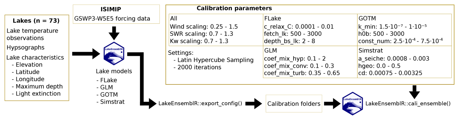
Figure 2 Workflow of the calibration; for a description and units of the calibrated parameters, see Table 1. The light extinction coefficient (Kw) for each specific lake was calibrated by multiplying the default value by a scaling factor in the range from 0.7 to 1.3.

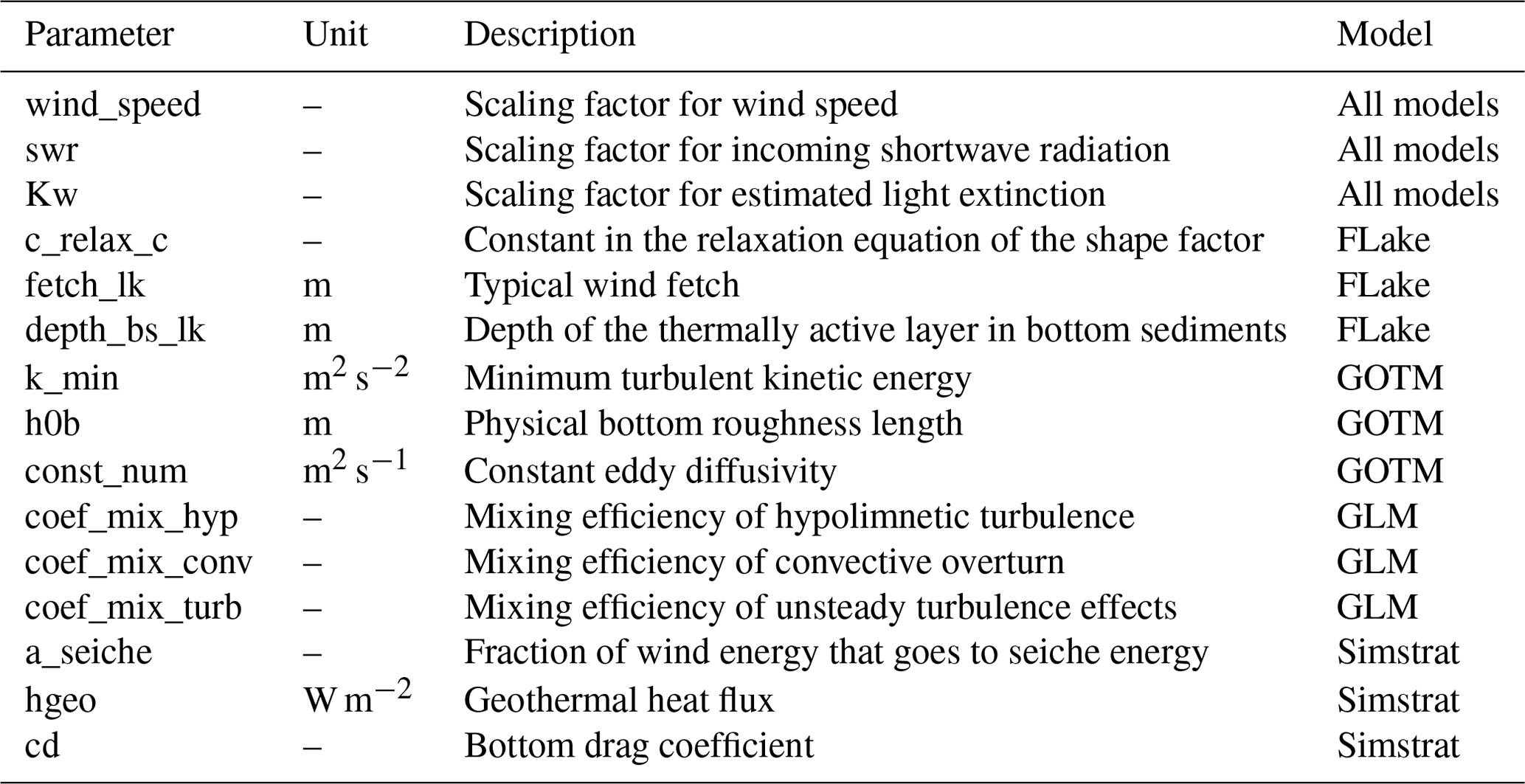
Finally, we ran the calibration using a Latin hypercube approach (see, e.g., Mckay et al., 2000). Here, we chose six parameters for each model: three model-specific parameters and three scaling factors (for wind speed, incoming shortwave radiation, and the estimated light extinction coefficient, respectively; Table 1). For the model-specific parameters, we chose parameters that are commonly used to calibrate these models, based on the literature (see Moore et al., 2021) and discussions on the parameter range held by the Lake Modelling working group at the GLEON All Hands' Meeting in 2020 and 2021 (Hansen et al., 2018). We sampled and ran the four models for 2000 parameter sets, and we calculated four performance metrics over all water temperature observations for each of the parameter sets: root-mean-square error (RMSE), Nash–Sutcliffe model efficiency (NSE), Pearson correlation coefficient (R), and mean error (bias).

Table 1 Description of the calibrated parameters. For the range of the parameters, see Fig. 2.

2.5 Global sensitivity analysis

Based on the sampled parameter sets and the calculated performance metrics, we performed a delta moment-independent sensitivity analysis (Plischke et al., 2013; Borgonovo, 2007) for each performance metric per lake per model, using the SALib Python library (Iwanaga et al., 2022; Herman and Usher, 2017). The analysis calculates two sensitivity measures, the moment-independent δ and variance-based Sobol' S₁. The delta moment-independent measure δ considers the entire distribution of the model output instead of a particular moment (e.g., variance) by calculating the difference between the unconditional and conditional cumulative distribution functions of the simulated model output, whereas the variance-based first-order Sobol' index S₁ calculates a parameter's influence on the variance of the simulated model output (Plischke et al., 2013; Borgonovo, 2007). As this study was interested in identifying the most important parameters (i.e., factor prioritization setting), we followed the recommendations of Borgonovo et al. (2017) and used both variance-based and moment-independent measures to increase the robustness when inferring which parameters are most important when simulating water temperatures. In addition to the six calibrated parameters, we included a dummy parameter that had no influence on the model output in the sensitivity analysis, which we sampled from a uniform distribution ranging from zero to one. In theory, this dummy variable should have a sensitivity of zero; however, due to the numerical approximation of the sensitivity measures, it can have small nonzero values. This can be used to approximate the error related to estimating sensitivity indices and thereby avoid classifying non-influential parameters as influential. This approach has been used in previous studies (e.g., Andersen et al., 2021; Khorashadi Zadeh et al., 2017). A resample size of 100 was used to compute confidence intervals on both sensitivity analysis metrics. To provide an estimate of potential parameter interactions, we additionally calculated the interaction indicator S_interaction (Borgonovo et al., 2017; Saltelli et al., 2000) that describes the fraction of model output variation apportioned by interactions:

$$\begin{array}{}\text{(13)}& S_{\mathrm{interaction}}=\mathrm{1}-\sum _{i=\mathrm{1}}^k{S}_i,\end{array}$$

where (S_i) is the first-order variance-based sensitivity measure (S₁) of parameter i out of k tested parameters.

3 Results

3.1 Model performance

The single best-performing model (out of the four applied models) for each lake reproduced observed water temperatures well for all 73 lakes, with a median RMSE of 1.2 °C and a median R of 0.98 (Fig. 3). The variation in error metrics between the best- and worst-performing model for each lake was rather small, e.g., a standard deviation of 0.5 °C or less in the RMSE (Fig. S3). Simstrat performed the best in most lakes in terms of the RMSE, R, and NSE, while GLM performed best in most lakes with respect to the bias (Fig. 3). However, all four models outperformed the others in at least some of the lakes. In over 90 % of all lakes, at least two different models performed best for different metrics.

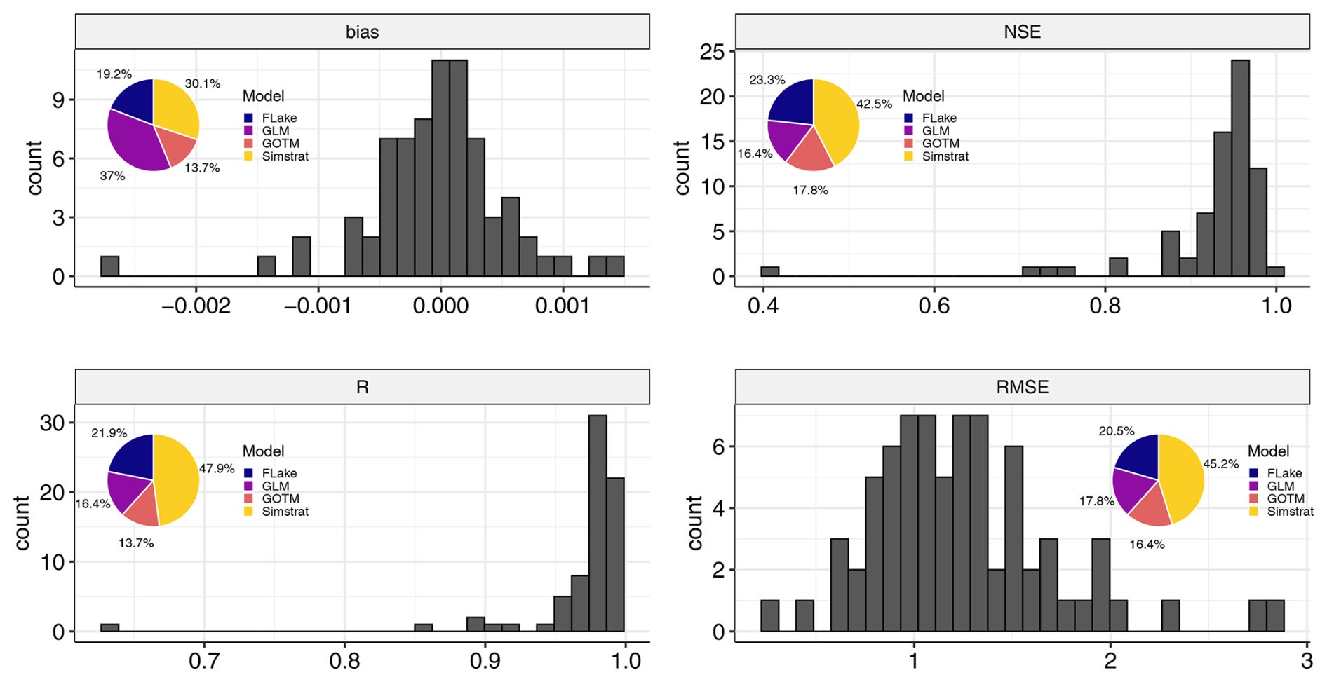
Figure 3 Distribution of the four evaluated performance metrics for the single best-performing model over the 73 lakes. The pie charts show how often the different models performed best per lake and metric. The units for the RMSE and bias are degrees Celsius.

Following the cluster analysis, we classified the lakes into five clusters. We visually compared the characteristics of the clusters (Fig. S4) and characterized them according to their most noticeable features: “deep” (n = 3), “medium temperate” (n = 25), “small temperate” (n = 32), “large shallow” (n = 4), and “warm” lakes (n = 9) (Fig. 1). Model performance was comparable among the clusters, although the deep lakes had a lower RMSE, whereas medium, small temperate, and large shallow lakes performed best in terms of the NSE and R (Fig. S5). When considering the four models separately, the overall better performance of Simstrat was mostly due to its better performance in the deep and medium temperate lakes, compared with the other models. In the other three clusters, the four models performed similarly (Fig. S6).

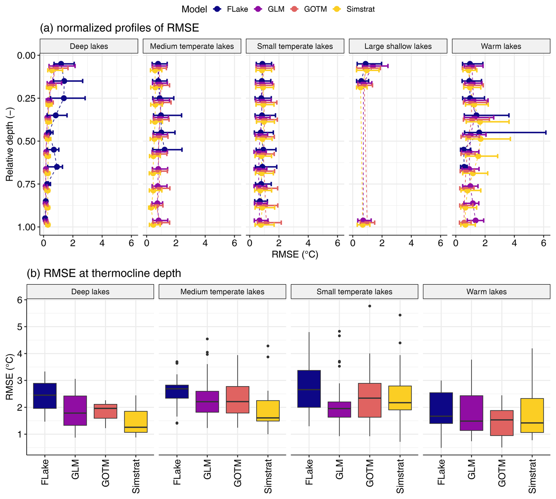
Figure 4 Depth distribution of the root-mean-square error (RMSE) for the models and lake clusters (a) and box plots of the RMSE at the thermocline depth (b). The depth was normalized to the depth of the deepest measurement (with 0 being the surface and 1 being the deepest point) and then binned in steps of 0.1. The points represent the median RMSE over all profiles, and the error bars present the 25 % to 75 % quantiles. If water temperatures deeper than 3 m were unavailable, no thermocline was calculated.

We calculated the ensemble mean by taking the arithmetic mean of the four models for each time step and depth individually. We then tested this as an additional predictor for water temperature and calculated its performance in terms of the RMSE. For the majority of lakes, the ensemble mean performed better than any single model (Fig. S7). This is especially visible in the medium temperate, small temperate, and large shallow lakes, where the ensemble mean performed best for the majority of lakes. The cases where the ensemble mean did not perform better than each single model were often lakes in which a single model performed notably better or worse than the other three models.

Looking at the distribution of the model error in terms of the RMSE over the water column depth (Fig. 4a), we can see that Simstrat performed better over all depths for the medium temperate lakes. In the deep lakes, FLake performed considerable worse than the other three models, especially at intermediate depths. For the other three models, the error increased towards the surface. For all four models in the large shallow lakes, the error was larger at the surface, while the error was largest at intermediate depths for the warm lakes.

From the observed water temperatures, we calculated the thermocline depth and then chose the simulation–observation pairs closest to that depth to estimate the RMSE at the thermocline temperature (Fig. 4b). For the large shallow lakes, no thermocline could be calculated. Simstrat performed best at the thermocline depth for deep, medium temperate, and warm lakes: its performance for deep and medium temperate lakes was about 0.5 °C better, while it was only about 0.1 °C lower than the next best model for warm lakes. For small temperate lakes GLM performed better, with a median RMSE that was about 0.3 °C lower than the next best model. FLake performed most poorly at the thermocline depth for all lake clusters.

3.2 Parameter sensitivity

From the calibration runs using the Latin hypercube approach, we calculated the moment-independent measure δ and the variance-based first-order measure S₁ for each combination of models, performance metrics, and lakes (Fig. 5). We saw a similar ranking of the most influential model parameters on most combinations of models, performance metrics, and lakes for δ and S₁. For almost all lakes, the same three to four parameters were classified as sensitive: the scaling factors for wind speed, shortwave radiation, and light extinction as well as k_min for GOTM. Moreover, one or two of these parameters accounted for more than 75 % of the sum of the sensitivity measures for most lakes (Fig. S8). Most often, these were meteorological scaling factors, which are not model-specific, with the exception of GOTM, in which k_min was most sensitive. Additionally, the light extinction coefficient and other model-specific parameters appeared to be sensitive in a couple of lakes (Fig. 5), although to a lesser degree.

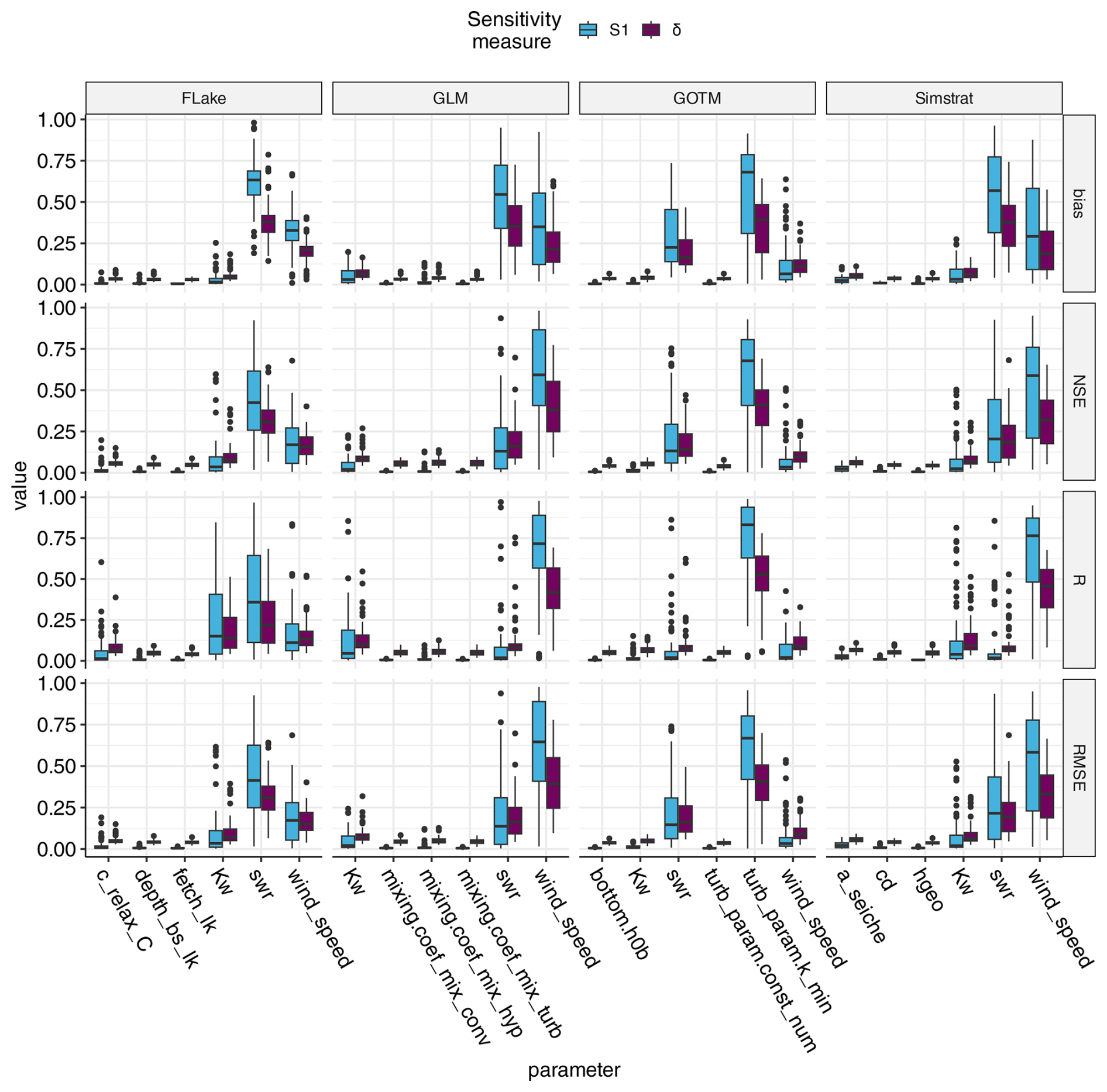
Figure 5 Box plot of the two calculated sensitivity measures for each parameter of the four models and for the four calculated performance metrics over all lakes.

For most models and performance metrics, interaction effects accounted for less than 20 % of the variation in model performance, although interactions were relevant for specific models and lake groups (Fig. 6). For instance, interactions were relevant for GLM modeling deep lakes and, to a lesser degree, for GLM and Simstrat modeling large shallow lakes. In contrast, increased parameter interactions were observed for FLake, especially for the NSE and RMSE, for all lake clusters except deep lakes. We highlight that, especially in lakes with shorter time series of observed water temperature data, the interaction measure was larger (Fig. S9). Interactions were low for the bias for all models and lake clusters.

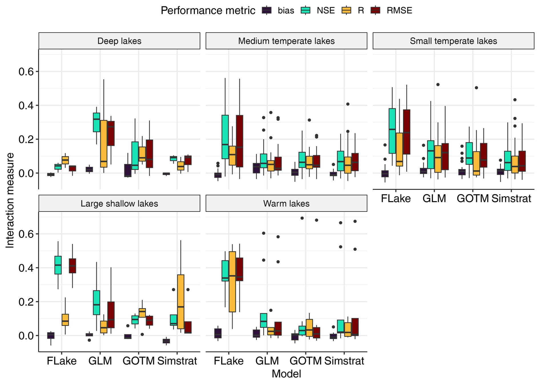
Figure 6 Box plot of the interaction measure of the first-order sensitivity metric for the four models and performance metrics over all lakes.

3.3 Distribution of best parameter values

Looking at the parameter values from the best-performing parameter sets, the optimal meteorological scaling factors differed between models. Especially GOTM showed a different behavior from the other models, with lower wind speed scaling factors and a higher shortwave radiation scaling factor (Fig. 7). The lake clusters also differed with respect to the optimal scaling factors, although their effects seemed model-specific. Differences in extinction factor scaling were less clear than the meteorological scaling factors, but GLM preferred a higher extinction factor in large shallow lakes, whereas FLake preferred a higher extinction factor in deep and medium temperate lakes. Most model-specific parameters had a low sensitivity, but some still showed markedly different behavior among clusters (Fig. S10). The single model-specific parameter with high sensitivity, GOTM's k_min, had distinctly lower values in small temperate lakes. For both the scaling factors and the model-specific parameters, we saw that the outcome was different depending on which performance metric was used to select the best parameter set (see Fig. S11).

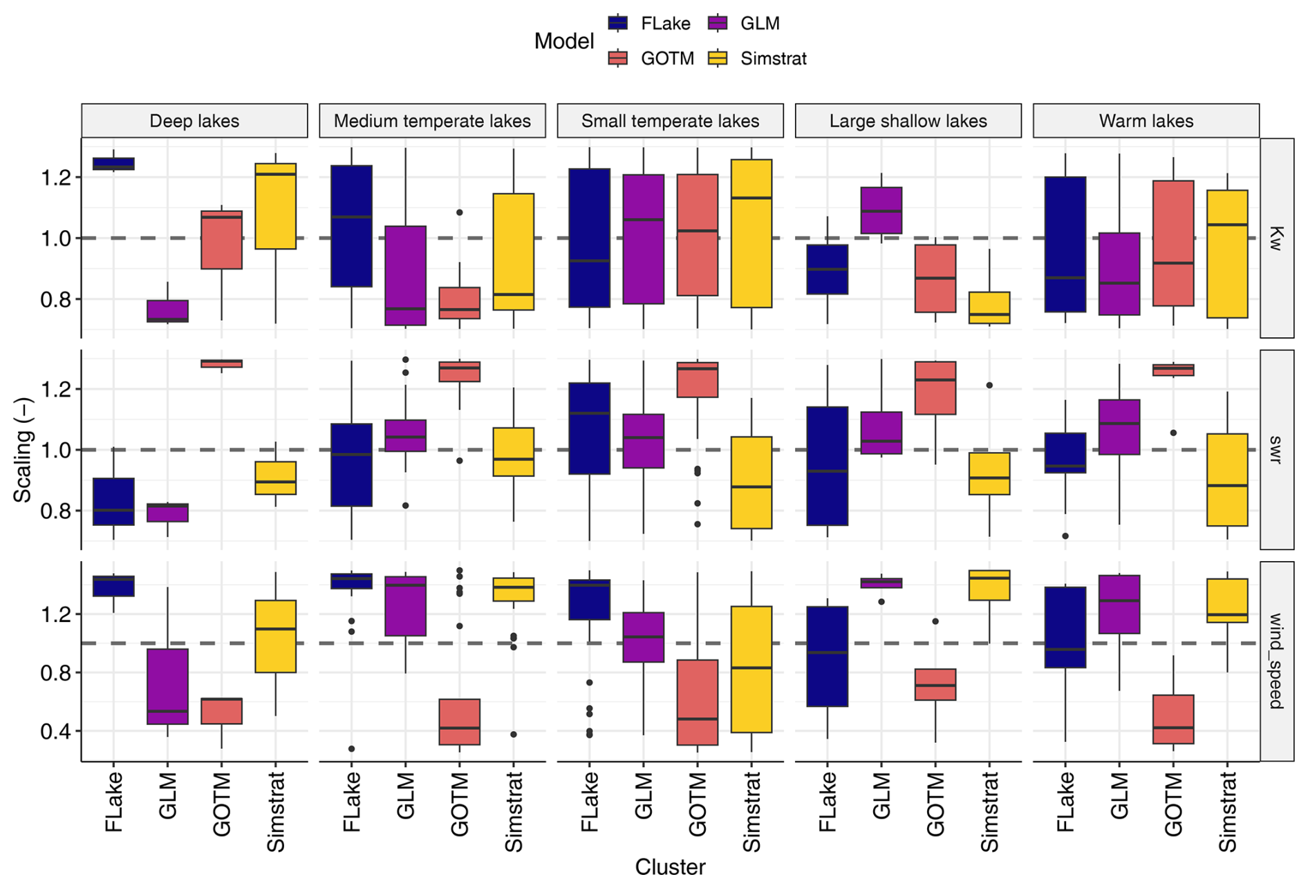
Figure 7 Distribution of the wind speed, shortwave radiation (swr), and light extinction (Kw) scaling factors, faceted by model and lake cluster. The light extinction scaling factors are normalized to each lake's default light extinction value. The optimal values are determined only based on the RMSE.

4 Discussion

Using a standardized and computationally efficient calibration approach (2000 model runs per model and lake), we were able to reproduce water temperature to a sufficient accuracy for 73 lakes across the globe. For 95 % of the lakes, the single best-performing model had an RMSE below 2 °C with a median of all performing models at 1.2 °C. Model-specific performance (Table S3) naturally showed higher error values but remained below 2 °C for most lakes and models. Compared to a previous ISIMIP simulation round, the performance in terms of median RMSE was similar (ISIMIP 2b; Golub et al., 2022), although GLM, GOTM, and Simstrat performed slightly worse and FLake performed slightly better in our simulation. Possible reasons for this could be the different meteorological forcing, the composition of lakes, and a different calibration approach. In comparison to two other multi-lake applications of gridded meteorological data, our calibration performed similarly (ALBM; Guo et al., 2021) or better (GLM; Read et al., 2014) in terms of the RMSE. In over 40 % of all lakes, the ensemble mean performed better than any single model in terms of the RMSE. Similar to previous studies using an ensemble framework (e.g., Feldbauer et al., 2022; Ladwig et al., 2023), it seems that the ensemble mean is a good predictor for water temperature dynamics. However, when using a larger global dataset, we showed that employing the simple arithmetic average as an ensemble mean did not increase performance for a subset of lakes. As, in many of these cases, a single model performed notably better or worse than the other ensemble members, a step forward could be to use other averaging techniques to make better use of the ensemble simulation. Such approaches already exist in other fields, like the reliability ensemble averaging method (REA) for climate simulations (Giorgi and Mearns, 2002).

Model performance showed a distinct pattern over the five lake clusters: when looking at the RMSE, general model performance in deep lakes was better, whereas it was worse in large shallow lakes compared with the other clusters. However, both deep and warm lakes showed poorer model performance when considering the NSE (Fig. S5). We attribute the model performance in deep lakes (n = 3) to the low variation in the deep-water temperatures, which the models could approach closely (a low RMSE), whereas the relatively small temporal variations were harder to simulate (i.e., poorer performance in terms of the NSE). The reduced model performance in terms of the RMSE for large shallow lakes (n = 4) was likely due to the intense interaction with the atmosphere (worsened by the use of gridded instead of locally observed meteorological data), while the lower NSE in warm lakes (n = 9) can be explained by the reduced seasonality in weather forcing data, and thus a harder-to-achieve high performance in metrics relying on a temporal trend. Other performance differences between lake clusters, such as that in the bias, or any differences between the two largest clusters (small temperate and medium temperate lakes) were marginal. These two largest clusters covered 78 % of the lakes in the dataset, which is in line with the higher presence of temperate lakes in the ISIMIP dataset. However, the unequal division of lakes over the clusters does skew the comparison, as conclusions regarding differences in other clusters are based on lower sample sizes.

To discuss how individual model performance is related to the underlying equations and design, we first need to acknowledge the limitations of this analysis: (a) parameter selection was limited and had identical ranges across models, which could cause a bias for models that would need specific adjustments during calibration, and (b) we neglected any inflows and outflows. Observed water temperature fluctuations caused by entrainment or withdrawal could be apparent in the training data, and models could replicate them by manipulating other processes (internal shear or mixing), thereby neglecting the actual hydrodynamic flow processes which caused the abovementioned temperature fluctuations. We note that the level of complexity in the process formulations for inflows and outflows varies across the models. Putting these caveats due to the standardized methodology aside, 1D lake models have improved performance compared with single 0.5D lake models, like FLake, for deep and medium temperate lakes. Here, all 1D lake models better replicated water temperatures in the surface layers (relative depths up to 0.75 and about 0.5 for deep and medium temperate lakes, respectively; Fig. 4a), underscoring that their respective algorithms, wind-induced mixing in GLM and computation of TKE in GOTM and Simstrat, outperform the shape assumptions that underlie FLake to replicate depth-specific near-surface water temperature dynamics. Additionally, their higher light extinction near the atmosphere–water surface interface due to attenuation of nonvisible light could also be a factor in their improved depth-specific simulation of water temperature in medium temperate and deep lakes. Below the epilimnion, at the thermocline, Simstrat outperforms the other models (Fig. 4b) in deep and medium temperate lakes. This underscores the importance of accounting for energy sources below the epilimnion. We assume that Simstrat's seiche excitation and damping parameterization has more accurately simulated the availability of TKE at these metalimnetic depths, which were not reached by wind shear stress originating from the atmosphere–water interface. We reinforced this hypothesis by performing additional simulations with a_seiche set to 0, which led to poorer model performance of Simstrat (see the Supplement for details). This emphasizes the importance of implementing deep-water mixing algorithms in 1D lake models to account for mixing at intermediate depths, which are usually characterized as quiet with respect to turbulent fluxes (Wüest and Lorke, 2003). In the hypolimnion, models performed similarly, with Simstrat only producing slightly better replications of the deep-water temperature in medium temperate lakes.

For the calibration of the lake models, we took an approach commonly used in applied studies where scaling factors for wind speed and shortwave radiation, the extinction coefficient, and a few model-specific parameters are calibrated (e.g., Ayala et al., 2020; Weber et al., 2017). Additionally, we used the output of the calibration to conduct a global sensitivity analysis of the calibrated parameters. We selected the model-specific parameters and the ranges for all parameters based on previous studies and expert knowledge, but we acknowledge that this approach is somewhat limited compared with an extensive sensitivity analysis including all model parameters. However, to our knowledge, there have only been a few studies that have looked at the sensitivity of the parameters of the used models (e.g., GLM – Bruce et al., 2018; GOTM – Andersen et al., 2021), and even those did not include all model parameters. Moreover, the model performance of all four investigated performance metrics was comparable to similar studies (e.g., Golub et al., 2022), despite using only a selection of parameters for the calibration. The sensitivity analysis revealed that, for most lakes and models, the most sensitive parameters were the scaling factors. Thus, it could be reasoned that only calibrating the scaling factors could be sufficient for similar applications. The clear exception here is GOTM, for which the minimum turbulent kinetic energy level (k_min) was shown to be highly sensitive for all lake clusters besides the large shallow lakes (Fig. S12). In fact, k_min was so important that it could dominate the other scaling factors, leading to different overall patterns in the calibrated parameters with lower values for the wind speed scaling across all lakes, compared with the other models (Fig. 7). This warrants future caution when calibrating k_min, as this parameter, which directly manipulates background turbulent kinetic energy and, therefore, turbulent transport, is highly sensitive. A way forward to address this could be the use of local field measurements to restrict the lake-specific range of estimates for k_min.

Specifically, the range for the wind speed scaling that we used in the calibration was quite large (0.25–1.5); however, even with this range, the best-performing estimates are located close to the limits for some of the lakes. An explanation for this large range of scaling factors is that we used forcing from bias-corrected (to global data sources, not data measured above the lakes; Lange, 2019) reanalysis data with a grid size of 0.5° × 0.5°. Local wind fields can have large variations; especially for lakes, sheltering plays an important role, as lakes are, by definition, located in depressions in the landscape. Simultaneously, larger lakes can act as smoother surfaces with higher near-surface wind speeds compared with surrounding areas. We could not highlight any relations between the best parameter values for the wind speed scaling factors and lake size, which could imply that the gridded weather data mask any effects of lake size. This highlights that there is still potential to enhance the model quality of local wind speed (Tan et al., 2024). The use of daily aggregated wind speeds also requires caution, as the mechanic energy transferred to the water is a cubic function of wind speed (Wüest et al., 2000); therefore, averaging of the measured wind speed can lead to an underestimation of mixing. The large range for the wind speed (and shortwave radiation) scaling factors were probably partly responsible for their high sensitivity. In a setting with locally observed meteorological forcing data, the model-specific parameters might become more influential if meteorological forcing variables can be better constrained. Previous studies used this approach in one or a few lakes (e.g., Guseva et al., 2020; Guo et al., 2021), but it would be beneficial to compile such data for a larger number of lakes, similar to the present study. Reducing the strong influence of meteorological scaling factors could facilitate the identification of optimal models for different clusters. If observations are not available, improvements in downscaling methods from global products to weather conditions at the lake surface might also partially achieve this. Similarly, the use of hourly meteorological forcing could result in more realistic patterns in wind-driven or convective mixing (Ayala et al., 2020).

We highlight that both sensitivity metrics and calibrated parameter values were strongly influenced by the chosen performance metrics (see, e.g., Figs. 5 and S11). This means that the model configuration would be different depending on which performance metric is chosen (except for the RMSE and NSE, which will lead to the same set of parameters). Therefore, it is important to choose the model performance metric with care, as they capture different aspects of the performance (see, e.g., Jachner et al., 2007). For a more thorough assessment of the choice of performance metrics, model validation at multiple levels of complexity could be performed (Hipsey et al., 2020).

Interaction between parameters was larger for FLake compared with the other models, except for deep lakes, where GLM and GOTM showed larger interactions, and large shallow lakes, where FLake, GLM, and Simstrat showed interactions (Fig. 6). For the lakes with high interaction measures, we found the interdependence of two or more parameters, most notably wind speed scaling and shortwave radiation scaling as well as, in some cases, the light extinction factor or model-specific parameters. A higher shortwave radiation increases the near-surface water temperatures and can promote stratification, while a higher wind speed has largely the opposite effect. The effect of wind on mixing dynamics is notably different, so that the influence of the two variables can be separated given enough observations. We could see that the interaction measure was generally lower for GLM, GOTM, and Simstrat for lakes that had longer time series of observed water temperature (Fig. S9). However, for the simpler temperature algorithms in FLake, separating the impact of wind speed and shortwave radiation seems to be more difficult. Similarly, the lake type (identified by the clustering) seemed to influence the degree of interaction as well, perhaps extending to parameters other than the meteorological scaling factors, which is in line with the findings of Andersen et al. (2021).

The overall uncertainty in mechanistic simulations is usually related to uncertainty in the initial conditions, uncertainty in the driving data (both forcing data such as meteorology and data used for calibration such as water temperature), uncertainty in the model parameter values, and structural uncertainty in the process description (also called epistemic uncertainty) (Thomas et al., 2020; Scavia et al., 2021; Dietze, 2017). In this study, we aimed to explore the relationships between lake model performance, parameterization, and lake characteristics. For this, our main focus was on highlighting uncertainties related to parameter values and model structure. The uncertainty in the meteorological forcing was partly acknowledged by the inclusion of the scaling factors. However, because the scaling factors proved to be among the most sensitive parameters, they could have prevented the identification of an optimal model or patterns relating the parameterization of the models to the lake characteristics (if such an optimal fit exists). A way forward could be to reduce the uncertainty in the meteorological forcing data, and hence hopefully the sensitivity of the scaling factors, by using local meteorological observations instead of reanalysis data.

The sensitivity analysis and cluster analysis could provide hints towards improving global simulations without the need for model-specific calibration. The sensitivity analysis suggests that, with the parameter value ranges used here, the meteorological forcing data are the most influential with respect to reproducing observed lake water temperatures. Comparing the distributions of the best-performing parameter values between the lake clusters gives an indication of how to scale meteorological forcing (and potentially other less sensitive parameters) for certain lakes, which could result in an overall improvement with respect to simulating global lake water temperatures. For instance, the models showed clear improvement regarding model performance when scaling shortwave radiation and wind speed (Fig. 7). Sheltering and the cubic scaling of wind speed with mixing may account for some of the need to scale wind speed, whereas the scaling of shortwave radiation is less easily explained, although heat transport into the water column, shading, or another lack or excess of heat input may play a role. Regardless, an open question remains as to whether using the results of the cluster analysis to parameterize uncalibrated simulations should be done. A clear weakness of this study is the low sample size in some lake clusters (i.e., n = 3 for deep lakes). Furthermore, the model configuration can be problematic, as, for instance, the influential k_min parameter in GOTM had strong effects on mixing and would therefore interact with the meteorological scaling factors (more details on this can be found in the Supplement). Additionally, gridded data are supposed to give the best possible estimate of meteorological variables in a certain grid cell. Unless it can be shown that such data are skewed in a predictable way for lakes in particular, an adjustment of meteorological variables would mostly be needed to compensate for current sub-optimal process descriptions in lake models themselves. Thus, taking the above weaknesses into consideration, these findings raise the following related questions:

• Are gridded forcing data adequate to replicate lake-specific meteorological conditions and, thus, for use in the reproduction of a lake's thermal structure?

• If so, should improvements in current model performance be found solely by improving hydrodynamic process descriptions?

5 Conclusions

We calibrated four different lake temperature models to 73 lakes using bias-corrected reanalysis data as forcing and then estimated the sensitivity of the calibrated parameters. From the six parameters calibrated for each model, only two to three were sensitive. This suggests that it can be sufficient to calibrate the models using only a subset of parameters. We achieved good model performance compared with previous studies and underscored that, while some of the models performed better overall, each model outperformed the others in at least some lakes. We analyzed four different model performance metrics; for over 90 % of all lakes, at least two models performed best for different performance metrics. To understand the effect of lake characteristics on the model performance, we grouped the 73 lakes into five clusters representing different characteristics. We highlight that both the model structure and lake clusters influenced model performance. In general, the three 1D lake models (GLM, GOTM, and Simstrat) performed better than the 0.5D model (FLake). More specifically, Simstrat performed better with respect to simulating the water temperature at the depth of the thermocline than the other models. We attribute this to the seiche module included in Simstrat. From these findings, we conclude the following:

1. There is still room to improve model structure and process description of the 0.5D and 1D lake temperature models. Specifically, (better) representation of deep-mixing processes, e.g., internal seiches, could potentially benefit simulations results.

2. Using an ensemble of multiple lake models is beneficial, especially as the computational cost of using multiple models simultaneously is low for these 1D (0.5D) models. However, there is still room to take further advantage of the ensemble approach, e.g., by exploring weighted ensemble averaging techniques.

3. Even though we saw patterns in the best-performing parameter sets regarding the lake clusters, it is unclear if using this approach might improve uncalibrated simulations (i.e., simulations where no observations are available). This is mainly caused by the fact that we used gridded forcing data, and meteorological scaling factors (wind speed and shortwave radiation) were the most influential on the lake thermal structure, likely representing the importance of local orography and potential sheltering.

These conclusions serve as a baseline for understanding model sensitivity, and they can support further improvements and developments of water temperature simulations and, thus, a better assessment of global change in lakes and reservoirs. Additionally, these conclusions can be the basis of a broader discussion about model uncertainty – especially when using gridded forcing data – and its relation to model design and parameterization.