Non-asymptotic distributions of water extremes: much ado about what?

Non-asymptotic (𝒩𝒜) probability distributions of block maxima (BM) have been proposed as an alternative to asymptotic distributions of BM derived by means of classic extreme-value theory (EVT). Their advantage should be the inclusion of moderate quantiles, as well as of extremes, in the inference procedures. This would increase the amount of information used and reduce the uncertainty characterizing the inference based on short samples of BM or peaks over high thresholds. In this study, we show that the 𝒩𝒜 distributions of BM suffer from two main drawbacks that make them of little usefulness for practical applications. Firstly, unlike classic EVT distributions, 𝒩𝒜 models of BM imply the preliminary definition of their conditional parent distributions, which explicitly appears in their expression. However, when such conditional parent distributions are known or estimated, the unconditional parent distribution is readily available, and the corresponding 𝒩𝒜 distribution of BM is no longer needed as it is just an approximation of the upper tail of the parent. Secondly, when declustering procedures are used to remove autocorrelation characterizing hydroclimatic records, 𝒩𝒜 distributions of BM devised for independent data are strongly biased even if the original process exhibits low or moderate autocorrelation. On the other hand, 𝒩𝒜 distributions of BM accounting for autocorrelation are less biased but still of little practical usefulness. Such conclusions are supported by theoretical arguments, Monte Carlo simulations, and re-analysis of sea level data.

1 Introduction

In the last decades, the statistical analysis of hydroclimatic extremes has mainly relied on theoretical results and models developed by a branch of statistics called extreme-value theory (EVT) (Fisher and Tippett, 1928; Von Mises, 1936; Gnedenko, 1943; Jenkinson, 1955; Gumbel, 1958; Balkema and de Haan, 1974; Pickands III, 1975; Leadbetter, 1983; Smith, 1984; Davison and Smith, 1990; Coles, 2001; Beirlant et al., 2004; Salvadori et al., 2007). EVT describes the extremal behavior of observed phenomena by means of asymptotic probability distributions that are valid under certain assumptions about the parent process, such as large sample sizes n (i.e., n→∞ to guarantee asymptotic convergence), independence, and distributional identity. However, hydroclimatic records are commonly quite short and hardly ever behave as independent and identically distributed random variables. More often, hydroclimatic processes result from combinations of heterogeneous physical processes (e.g., Morrison and Smith, 2002; Smith et al., 2011, 2018) and exhibit autocorrelation (e.g., Kantelhardt et al., 2006; Wang et al., 2007; Serinaldi, 2010; Labat et al., 2011; Papalexiou et al., 2011; Serinaldi and Kilsby, 2016b; Lombardo et al., 2017; Iliopoulou et al., 2018; Markonis et al., 2018; Serinaldi and Kilsby, 2018; Serinaldi et al., 2018; Dimitriadis et al., 2021, and references therein), with their behavior being better described by stochastic processes incorporating such properties (e.g., Serinaldi and Kilsby, 2014a; Serinaldi and Lombardo, 2017a, b; Dimitriadis and Koutsoyiannis, 2018; Papalexiou, 2018; Koutsoyiannis, 2020; Papalexiou and Serinaldi, 2020; Koutsoyiannis and Dimitriadis, 2021; Papalexiou et al., 2021; Papalexiou, 2022; Serinaldi et al., 2022a; Koutsoyiannis, 2023, and references therein).

As a consequence, the lack of fulfillment of EVT assumptions affects the analysis of block maxima (BM) or over-threshold (OT) values as the BM and OT sample selection generally yields short sample sizes and does not remove the effects of autocorrelation and the possible heterogeneity of the generating mechanisms (see, e.g., Koutsoyiannis, 2004; Iliopoulou and Koutsoyiannis, 2019; Serinaldi et al., 2020b). Research in EVT has addressed these issues to some extent for the case of asymptotic and sub- or pre-asymptotic methods for the BM and OT processes (see Serinaldi et al., 2020b, and references therein for an overview).

On the other hand, parallel literature has focused on non-asymptotic (𝒩𝒜) approaches for BM, attempting to use as many observations as possible to infer the distribution of the largest values. 𝒩𝒜 distributions of BM include Todorovic distributions and their special cases (e.g., Todorovic, 1970; Todorovic and Zelenhasic, 1970; Lombardo et al., 2019), specifically the so-called metastatistical extreme value (MEV) distributions and their variants, such as the simplified MEV (SMEV; Marani and Ignaccolo, 2015; Zorzetto et al., 2016; De Michele and Avanzi, 2018; Marra et al., 2018; De Michele, 2019; Marra et al., 2019; Hosseini et al., 2020; Miniussi et al., 2020; Zorzetto and Marani, 2020).

Serinaldi et al. (2020b) explained the conceptual and analytical relationships among the above-mentioned 𝒩𝒜 distributions of BM in the context of compound distributions of order statistics and introduced compound beta-binomial distributions (βℬC) of BM in processes with stationary autocorrelation structure. βℬC distributions allow one to avoid declustering procedures required, for instance, by (S)MEV to obtain samples fulfilling the assumption of independence.

However, while the βℬC distributions allow a correct interpretation of the 𝒩𝒜 models of BM and their connections to their parent distributions, Serinaldi et al. (2020b) did not comprehensively explore the usefulness or lack thereof of 𝒩𝒜 models of BM in practical analysis. In this study, we further explore and discuss the extent of the redundancy of such models with respect to their parent distributions, as well as the actual lack of effectiveness in declustering procedures in the context of 𝒩𝒜-based analysis.

This paper falls into the class of so-called neutral (independent) validation–falsification studies (see, e.g., Popper, 1959; Boulesteix et al., 2018, and references therein), aiming to independently check the theoretical consistency in statistical methods applied in the analysis of hydroclimatic data (Lombardo et al., 2012, 2014, 2017, 2019; Serinaldi and Kilsby, 2016a; Serinaldi et al., 2015, 2018, 2020a, b, 2022b). We put emphasis on the common but misleading habit of seeking confirmation by iterating the application of a given method in relation to observed data whose generating processes are inherently unknown. In fact, if a method is technically flawed, its output will always be consistent across applications but systematically incorrect. In contrast, genuine neutral analysis calls into question the theory behind a method or model and checks it analytically and/or against challenging controlled conditions via suitable Monte Carlo simulations.

This study is organized as follows. In Sect. 2, we briefly review the main 𝒩𝒜 distributions of BM proposed in the literature and their relationship to the corresponding distributions of the parent process. Section 3 recalls the rationale for performing an extreme-value analysis and explains why the 𝒩𝒜 models of BM are conceptually redundant in this context. These aspects are further discussed in Sect. 4 using simple Monte Carlo simulations and by reanalyzing sea level data previously studied in the literature. Monte Carlo experiments in Sect. 5 investigate the performance of some 𝒩𝒜 models of BM under independence and serial dependence, as well as the effectiveness of declustering methods proposed to deal with autocorrelated time series and the reliability of some results previously reported in the literature. In Sect. 6, the problems concerning the use of 𝒩𝒜 models of BM for practical applications are placed within the wider context of a questionable approach to applied statistics in hydroclimatic studies. Conclusions are given in Sect. 7.

2 Overview of 𝒩𝒜 distributions of BM

To support our discussion, we firstly recall some basic theoretical results, referring to Serinaldi et al. (2020b) and the references therein for more details about the analytical derivation of the equations reported below. Under the assumption of an identical probability distribution, BM are the largest-order statistics (David and Nagaraja, 2004, p. 1) of a sequence of m random variables $Z_{\mathrm{1}},\mathrm{\dots },Z_m$ with the same cumulative distribution function (cdf) F_Z(z). If these variables are also independent, the cdf of BM Y in random samples of finite size m is

$$\begin{array}{}\text{(1)}& \begin{array}{rl}{F}_Y\left(z\right)=& \sum _{i=m}^m\left(\begin{array}{c}m\\ i\end{array}\right)F_Z^i\left(z\right)[\mathrm{1}-F_Z(z){]}^{m-i}=F_Z^m(z)\\ =& \mathrm{1}-F_{\mathcal{B}}(m-\mathrm{1};m,F_Z(z\left)\right)\\ =& F_{\mathcal{B}}(\mathrm{0};m,\mathrm{1}-F_Z(z\left)\right)\\ =& F_{\mathit{\beta }}\left(F_Z\right(z);m,\mathrm{1}),\end{array}\end{array}$$

where F_ℬ and F_β are the binomial and beta cdf's, respectively. Under the assumption of serial dependence, the distribution of BM in finite-sized blocks is unknown as it depends on the m-dimensional joint distribution of the m variables forming a block (Todorovic, 1970; Todorovic and Zelenhasic, 1970). Closed-form solutions do exist for the case of Markovian processes, whereby the joint distribution is bivariate (Lombardo et al., 2019). For high-order dependence structures, the 𝒩𝒜 distribution of BM can be approximated by an extended beta–binomial distribution βℬ (Serinaldi et al., 2020b, Sect. 2.2):

$$\begin{array}{}\text{(2)}& \begin{array}{rl}{F}_Y\left(z\right)=& {\displaystyle \frac{\mathrm{B}\left(\mathit{\alpha }\right(z),m+\mathit{\beta }(z\left)\right)}{\mathrm{B}\left(\mathit{\alpha }\right(z),\mathit{\beta }(z\left)\right)}}\\ =& F_{\mathit{\beta }\mathcal{B}}(\mathrm{0};m,\mathrm{1}-F_Z(z),{\mathit{\rho }}_{\mathit{\beta }\mathcal{B}}(F_Z\left(z\right),\mathit{\rho }\left)\right),\end{array}\end{array}$$

where F_βℬ is the βℬ cdf; $\mathrm{B}(\cdot ,\cdot )$ is the complete beta function (Arnold et al., 1992, pp. 12–13); and ρ_βℬ(z) is known as the “intra-class” or “intra-cluster” correlation, which depends on F_Z(z) and the autocorrelation function (ACF) of the parent process $\mathit{\{}{Z}_i{\mathit{\}}}_{i=\mathrm{1}}^m$, denoted as ρ. When the parent process Z_i is serially uncorrelated (ρ_βℬ=0), Eq. (2) yields Eq. (1) as a particular case.

The process Z is named the “parent” as it is the stochastic process whose distribution F_Z appears in the expression of the distribution of BM F_Y, and it could have no strict physical meaning. For example, the parent process used to build the distribution of BM for precipitation or streamflow sampled at a given timescale (e.g., daily) could be the process of observations over any threshold guaranteeing the selection of at least one observation per block. Therefore, inter-arrival times of the observations z are always smaller than or equal to the m time steps corresponding to the block size. As a limiting case, Z can obviously be the complete streamflow or rainfall process sampled at the finest timescale (e.g., daily).

As discussed in more depth in the next sections, every distribution of BM (asymptotic or non-asymptotic) provides just an approximation of the upper tail of the distribution of the parent process. Equations (1) and (2) indicate that two parent processes can have the exact same marginal distribution, but the expression of the corresponding 𝒩𝒜 model of BM approximating the upper tail of F_Z might be different according to the presence or absence of serial dependence. In other words, serial dependence influences the patterns of the observations z within each block and, therefore, the sequences of BM and the form of their 𝒩𝒜 distribution F_Y. On the other hand, F_Z is unaffected by serial dependence as it describes the distribution of Z, which does not imply any operation (aggregation, average, or BM selection) over a time window (block).

The assumption of intra- or inter-block distributional identity can be relaxed by resorting to the concept of mixed or compound distributions, which integrate (average) over the parameter space of the parent distribution under the assumption that these parameters can change within or between each block (Marra et al., 2019; Serinaldi et al., 2020b). For instance, such changes or fluctuations can reflect different physical generating mechanisms (e.g., convective and frontal weather systems generating storms in different seasons) or inter-block sampling uncertainty related to still unidentified physical processes, which therefore need a stochastic description. A general compact form of this class of models can be written as

$$\begin{array}{}\text{(3)}& F_Y\left(z\right)=\sum _{l=\mathrm{0}}^{\mathrm{\infty }}\underset{{\mathrm{\Omega }}_{\mathit{\theta }}}{\int }{G}_l(z;\mathit{\theta })g(l,\mathit{\theta })\mathrm{d}\mathit{\theta }=\mathbb{E}\left[G_L\right(z;\mathbf{\Theta }\left)\right],\end{array}$$

where $G_l(z;\mathit{\theta })=\mathbb{P}[Z_{\mathrm{1}}\le z\wedge Z_{\mathrm{2}}\le z\wedge \mathrm{\dots }\wedge Z_l\le z|L=l,\mathbf{\Theta }=\mathit{\theta }]$ is the joint distribution of the parent process accounting for intra-block dependence, Ω_θ is the state space of parameter vector θ, and 𝔼[⋅] is the expectation operator. G_l is integrated (averaged) over the number of observations L in each block of size m and the parameters Θ, which are treated as random variables with a joint probability density function (pdf) g(l,θ). Equation (3) is a generalization of Todorovic distributions, incorporating possible inter-block fluctuations of parameters of the joint distribution of parent process Z.

Since high-dimensional joint distributions G_l are difficult to handle and fit, the general model in Eq. (3) can be approximated by a compound version of the βℬ distribution in Eq. (2) for high-order dependence structures, resulting in the following compound βℬ model (βℬC) (Serinaldi et al., 2020b, Sect. 5.2):

$$\begin{array}{}\text{(4)}& \begin{array}{rl}{F}_Y\left(z\right)\cong F_{\mathit{\beta }\mathcal{B}\mathrm{C}}\left(z\right):=& \sum _{l=\mathrm{0}}^{\mathrm{\infty }}\underset{{\mathrm{\Omega }}_{\mathit{\rho }}}{\int }\underset{{\mathrm{\Omega }}_{\mathit{\theta }}}{\int }{F}_{\mathit{\beta }\mathcal{B}}(\mathrm{0};l,\mathrm{1}-F_Z(z;\mathit{\theta }),\\ & {\mathit{\rho }}_{\mathit{\beta }\mathcal{B}}\left(F_Z\right(z;\mathit{\theta }),\mathit{\rho })\left)g\right(l,\mathit{\rho },\mathit{\theta })\mathrm{d}\mathit{\rho }\mathrm{d}\mathit{\theta }\\ =& \mathbb{E}\left[F_{\mathit{\beta }\mathcal{B}}\right(\mathrm{0};l,\mathrm{1}-F_Z(z;\mathbf{\Theta }),\\ & {\mathit{\rho }}_{\mathit{\beta }\mathcal{B}}\left(F_Z\right(z;\mathbf{\Theta }),\mathbf{P})\left)\right],\end{array}\end{array}$$

where F_βℬC is the βℬC cdf, ρ is the correlation function of the parent process Z, and Ω_ρ is its state space. Under the assumption of independence (ρ=0), the βℬ distribution is reduced to a binomial distribution (which can also be written in the form of a beta distribution), and Eq. (4) yields MEV models as special cases:

$$\begin{array}{}\text{(5)}& \begin{array}{rl}{F}_Y\left(z\right)=& \sum _{l=\mathrm{0}}^{\mathrm{\infty }}\underset{{\mathrm{\Omega }}_{\mathit{\theta }}}{\int }{F}_{\mathcal{B}}(\mathrm{0};l,\mathrm{1}-F_Z(z;\mathit{\theta }\left)\right)g(l,\mathit{\theta })\mathrm{d}\mathit{\theta }\\ =& \sum _{l=\mathrm{0}}^{\mathrm{\infty }}\underset{{\mathrm{\Omega }}_{\mathit{\theta }}}{\int }{F}_{\mathit{\beta }}\left(F_Z\right(z;\mathit{\theta });l,\mathrm{1})g(l,\mathit{\theta })\mathrm{d}\mathit{\theta }\\ =& \sum _{l=\mathrm{0}}^{\mathrm{\infty }}\underset{{\mathrm{\Omega }}_{\mathit{\theta }}}{\int }{F}_Z^l(z;\mathit{\theta })g(l,\mathit{\theta })\mathrm{d}\mathit{\theta }.\end{array}\end{array}$$

Analogously to Eqs. (1) and (2), Eqs. (4) and (5) approximate the upper tail of the distribution of the parent process Z:

$$\begin{array}{}\text{(6)}& F_Z\left(z\right)=\underset{{\mathrm{\Omega }}_{\mathit{\theta }}}{\int }{F}_Z(z;\mathit{\theta })g\left(\mathit{\theta }\right)\mathrm{d}\mathit{\theta }.\end{array}$$

This is, in itself, a compound distribution (averaged over the parameter space) and should not be confused with the conditional distributions F_Z(z;θ), which depend on the parameters. F_Z in Eq. (1) is also unaffected by serial correlation, which, in turn, changes the form of the corresponding 𝒩𝒜 distribution F_Y of BM. As mentioned above, we can have two parent processes with identical F_Z and different F_Y depending on the presence or absence of serial dependence. Equations (4) and (5) are quite general and account not only for inter-block fluctuations via g(θ) but also for intra-block variability (such as different physical generating mechanisms and/or seasonal fluctuations acting at the intra-block scale) assuming that the conditional distributions F_Z(z;θ) are compound or mixed – that is,

$$\begin{array}{}\text{(7)}& F_Z(z;\mathit{\theta })=\underset{{\mathrm{\Omega }}_{\mathit{\vartheta }}}{\int }{F}_Z(z;\mathit{\vartheta },\mathit{\theta })g(\mathit{\vartheta };\mathit{\theta })\mathrm{d}\mathit{\vartheta },\end{array}$$

where g(ϑ;θ) describes the intra-block variability of ϑ (e.g., seasonal fluctuations or intra-annual weather system switching) conditioned on the inter-block status (e.g., El Niño or La Niña conditions spanning 1 or more years). Of course, g(ϑ;θ) is reduced to g(ϑ) if the intra-block fluctuations are assumed to be independent of inter-annual fluctuations. A typical example is the common assumption of year-to-year invariant seasonal patterns.

In the next sections, the models in Eqs. (1), (2), (4), and (5) are compared with the corresponding parent distributions. We stress that the models in Eqs. (4) and (5) must be compared with the corresponding compound parent distribution in Eq. (6), which accounts for the same intra- and/or inter-block variability. It is worth noting that the following discussion is fully general and valid for any 𝒩𝒜 model of BM requiring the preliminary knowledge or definition of F_Z(z;θ) and its use in the expression of F_Y. Hereinafter, the terms “𝒩𝒜 model or distribution of BM” and “𝒩𝒜 model or distribution” are used interchangeably to denote the same class of models.

3 Modeling extreme values: asking “why” before looking for “how”

Asymptotic distributions provided by EVT are the limit distributions of 𝒩𝒜 models under some assumptions concerning the nature of the marginal distribution and dependence structure of the parent process Z. In particular, it is well known that the generalized extreme value (GEV) and generalized Pareto (GP) distributions are the general asymptotes of the distributions of BM and peaks over thresholds (POTs), respectively, under the assumptions of independence (or certain types of weak dependence) and distributional identity (see, e.g., Leadbetter et al., 1983; Coles, 2001). Therefore, EVT models are fairly general and relatively easy to apply, mainly because they do not require a precise knowledge of F_Z (Leadbetter et al., 1983, p. 4), which, instead, explicitly appears in the expression of any 𝒩𝒜 model. This aspect has already been stressed in standard handbooks of applied statistics, such as that of Mood et al. (1974, p. 258), who stated (using our notation and setting L=m) “One might wonder why we should be interested in an asymptotic distribution of Y when the exact distribution, which is given by $F_Y\left(z\right)=F_Z^m\left(z\right)$, where F_Z is the c.d.f. [cumulative distribution function] sampled from, is known. The hope is that we will find an asymptotic distribution which does not depend on the sampled c.d.f. F_Z. We recall that the central-limit theorem gave an asymptotic distribution for $\stackrel{\mathrm{‾}}{Z}$ [sample mean] which did not depend on the sampled distribution even though the exact distribution of $\stackrel{\mathrm{‾}}{Z}$ could be found.”

Bearing in mind that Z and Y are two different processes (Serinaldi et al., 2020b, Sect 3.2), the usefulness and widespread application of asymptotic EVT models of BM and POTs stems from the fact that such distributions approximate (converge to) the upper tail of the distribution of the parent process Z without needing to know F_Z (under the above-mentioned assumptions) and only requiring a limited amount of information (i.e., BM and/or POT observations) instead of complete time series. This is paramount in practical applications as it allows the use of (i) a couple of general distributions (GEV and GP) supported by a theory that clearly identifies the range of the validity of such models and (ii) data that are more easy to collect and are more widely available worldwide compared to complete time series. For example, meteorological services provide most of the historical information on rainfall in terms of annual maximum values for specified durations to be used in the so-called intensity–duration–frequency (IDF) analysis. In these cases, we do not know F_Z, and we cannot fit it either as the data representing the whole rainfall process – and, therefore, F_Z – are not available. However, EVT states, for instance, that the GEV distribution asymptotically approximates the upper tail of F_Z independently of the form of F_Z (under certain constraints) based on theoretical results concerning the asymptotic behavior of $F_Y=F_Z^m$. EVT distributions independent of the form of F_Z are also useful when observations of Z are available, but defining a reliable model for F_Z is too difficult due to complexity of the hydroclimatic process of interest and its generating mechanisms.

Unlike asymptotic models, 𝒩𝒜 distributions require the preliminary knowledge or fit of F_Z, which explicitly appears in their expression. However, if we already know F_Z (or if we have a good estimate of it), we no longer need any 𝒩𝒜 distribution of BM as the latter provides only an approximation of the upper tail of the known or fitted F_Z. We do not even need any asymptotic model and/or, more generally, any model of BM or POTs as these are just processes extracted from the parent process Z, whose distribution F_Z already describes the whole state space, including the extreme values. The use of extreme-value distributions makes sense if and only if we do not have enough information on F_Z. Otherwise, the latter provides all the information needed to make statements about any quantile. In this context, $F_Z^m$ only plays a functional or intermediate role in theoretical derivations to move from F_Z to general asymptotic distributions independent of F_Z, to be used when F_Z is not available.

The same remarks hold true for any compound 𝒩𝒜 model such as βℬC and its special cases. In fact, these models require the preliminary inference of F_Z to derive distributions (compound versions of $F_Z^m$) that only approximate the upper tail of the previously estimated F_Z. It is easy to understand that such a procedure makes little sense in practical applications: why should one search for an approximation of the upper tail of a distribution that is already known or fitted? The use of compound 𝒩𝒜 models is not even justified by their mixing nature, which allows for averaging inter-block fluctuations of parameters. In fact, as further discussed below, such a mixing procedure can be directly applied to F_Z, thus obtaining a compound distribution of the parent process Z that can readily be used to make statements on any quantile, avoiding unnecessary 𝒩𝒜 approximations of the upper tail. This explains why 𝒩𝒜 models have not received much attention and why the recently proposed compound 𝒩𝒜 models are of little practical usefulness, if any. Their usefulness is mainly theoretical as they help explain the inherent differences between parent processes Z and BM processes Y, thus avoiding misconceptions and misinterpretations of different model outputs (see Serinaldi et al., 2020b).

4 Investigating circular reasoning and redundancy: do we need 𝒩𝒜 distributions of BM in practical applications?

While the concepts discussed in Sect. 3 should be well-known and self-evident, they seem to be systematically neglected in hydroclimatic literature dealing with 𝒩𝒜 models. Therefore, this section reports further discussion using some simple examples and real-world data re-analysis to highlight the relationship between 𝒩𝒜 models and the embedded distribution F_Z, thus showing concretely how the former provide only a redundant approximation of the upper tail of the latter.

4.1 Estimation of 𝒯-year events: recalling basic concepts to avoid inconsistencies

The first example is freely inspired by the work of Mushtaq et al. (2022), who searched for an approach to select the most suitable distribution F_Z of ordinary streamflow peaks (i.e., the parent process Z) between gamma and log-normal to be used to build MEV distributions F_Y for annual maxima (AM, i.e., the BM process Y). Here, we focus on the very primary logical contradiction (circular reasoning) of attempting to find a distribution F_Z to build F_Y as a function of F_Z to approximate the tail of F_Z itself, which is already known exactly. In this respect, to keep the discussion as simple and focused as possible but without the loss of generality, we do not use compound models but assume that the parent process is independent and identically distributed, following a gamma distribution. Compound models and the issues related to some MEV technicalities (such as the declustering method used to obtain apparently independent ordinary events) will be discussed in the second example. Concerning the first example, we firstly discuss the above-mentioned contradiction (circular reasoning) from a conceptual perspective and then provide visual illustration by means of Monte Carlo simulations.

4.1.1 The logic behind the estimation of return levels and the role of F_Z and F_Y

For the sake of illustration, let us suppose we have a hypothetical streamflow process sampled at a daily timescale, with us being interested in estimating a flow value that is exceeded, on average, every 𝒯 years, i.e., the so-called 𝒯-year return level corresponding to the 𝒯-year return period (see, e.g., Eichner et al., 2006; Serinaldi, 2015; Volpi et al., 2015, and references therein). Under the ideal situation where infinitely long records are available and, therefore, where F_Z and F_Y are known exactly, one can use the distribution of the parent process F_Z and determine the 𝒯-year return level as the quantile z_p that is exceeded with probability $p=\mathrm{1}/\left(\mathrm{365}\mathcal{T}\right)$, i.e., the value that is exceeded, on average, once in 𝒯 years = 365𝒯 d (leaving aside leap years). Since z_p is a quantile of the distribution F_Z, which describes the parent process at its finest available resolution (here, daily), it is unaffected by possible autocorrelation and clustering of 𝒯-year events (see Bunde et al., 2004, 2005; Serinaldi et al., 2020b, for an in-depth discussion). Note that this is the definition applied in the literature to compute the exact 𝒯-year return level used to assess the accuracy of 𝒩𝒜 models (see, e.g., Marani and Ignaccolo, 2015; Marra et al., 2018).

However, real-world records rarely span more than a few decades, and the data are not enough to obtain F_Z (and F_Y) and determine directly the 𝒯-year return level for high values of 𝒯, such as 100 or 1000 years. Therefore, an alternative approach is based on the distribution of AM, i.e., BM within relatively short intervals (i.e., 365 d). Of course, a virtually infinite sequence of BM defines their exact distribution. Such a distribution allows an approximate estimation of the 𝒯-year return level as the quantile that is exceeded with probability $\mathrm{1}/\mathcal{T}$ because 1 year is the finest timescale of AM. In other words, F_Y cannot provide information about events occurring more often than once in m days (e.g., once per year for AM) as this is the finest sampling frequency of BM for blocks of size m. This estimation of 𝒯-year return levels based on BM involves the joint exceedance probability within each block described by the intra-block joint distribution G_l (see Sect. 2), and, therefore, it is affected by autocorrelation (see Eichner et al., 2006, for a detailed discussion).

Therefore, the distributions of AM commonly used in hydroclimatology are only approximations of the upper tail of F_Z, and their estimation is justified if F_Z is unknown. This can happen if (i) we have no regular records of the parent process to reliably estimate F_Z or (ii) a faithful parameterization of F_Z is not so easy to determine due to the difficulties in accounting for various characteristics of the underlying process, such as cyclo-stationarity, different physical generating mechanisms, and other possibly unknown factors. In these cases, EVT comes into play, stating, for instance, that, under certain assumptions, the distribution of BM within relatively short intervals (e.g., 365 d) converges to one of the three asymptotic extreme-value models summarized by the GEV distribution independently of the exact form of F_Z. Of course, the approximate or partial fulfillment of EVT assumptions affects convergence. For example, autocorrelation and a lack of distributional identity slow convergence down (Koutsoyiannis, 2004; Eichner et al., 2006; Serinaldi et al., 2020b) and sometimes prevent it, resulting in degenerate models. These remarks explain why asymptotic models are such powerful tools that are widely applied in any discipline dealing with extreme values.

4.1.2 Visualizing the relationship between F_Z and F_Y

A simple example with a graphical illustration can help better clarify the difference between F_Z and F_Y (see Sect. 3.2 in Serinaldi et al., 2020b, for a formal discussion based on theoretical arguments). Let us assume that we have 365 × 10⁵ observations of an independent process Z following a gamma distribution with shape and scale parameters $\mathit{\kappa }=\mathit{\sigma }=\mathrm{2}$, representing, for instance, 10⁵ years of daily records of a hypothetical streamflow process (or a generic hydroclimatic process). These data allow one to build the empirical version of F_Z and F_Y and the corresponding pdf's f_Z and f_Y. In particular, Fig. 1 shows the empirical pdf's (Fig. 1a–c) and the return level plots (i.e., return level vs. return period; Fig. 1d–f) for two sub-samples of size 365 × 100 and 365 × 500 (i.e., 100 and 500 years, respectively) and for the whole data set (10 000 years). Figure 1 also displays the theoretical gamma pdf and return level curves, as well as empirical and theoretical 100-year quantiles (vertical lines). The 𝒯-year return levels are computed as the $(\mathrm{1}-\frac{\mathrm{1}}{\mathcal{T}})\cdot$ 100 % quantiles of the empirical cdf of AM and the $(\mathrm{1}-\frac{\mathit{\mu }}{\mathcal{T}})\cdot$ 100 % quantiles of the theoretical and empirical cdf's of the process Z, where $\mathit{\mu }=\mathrm{1}/\mathrm{365}$ can be interpreted as the inter-arrival time (in years) between two records of Z.

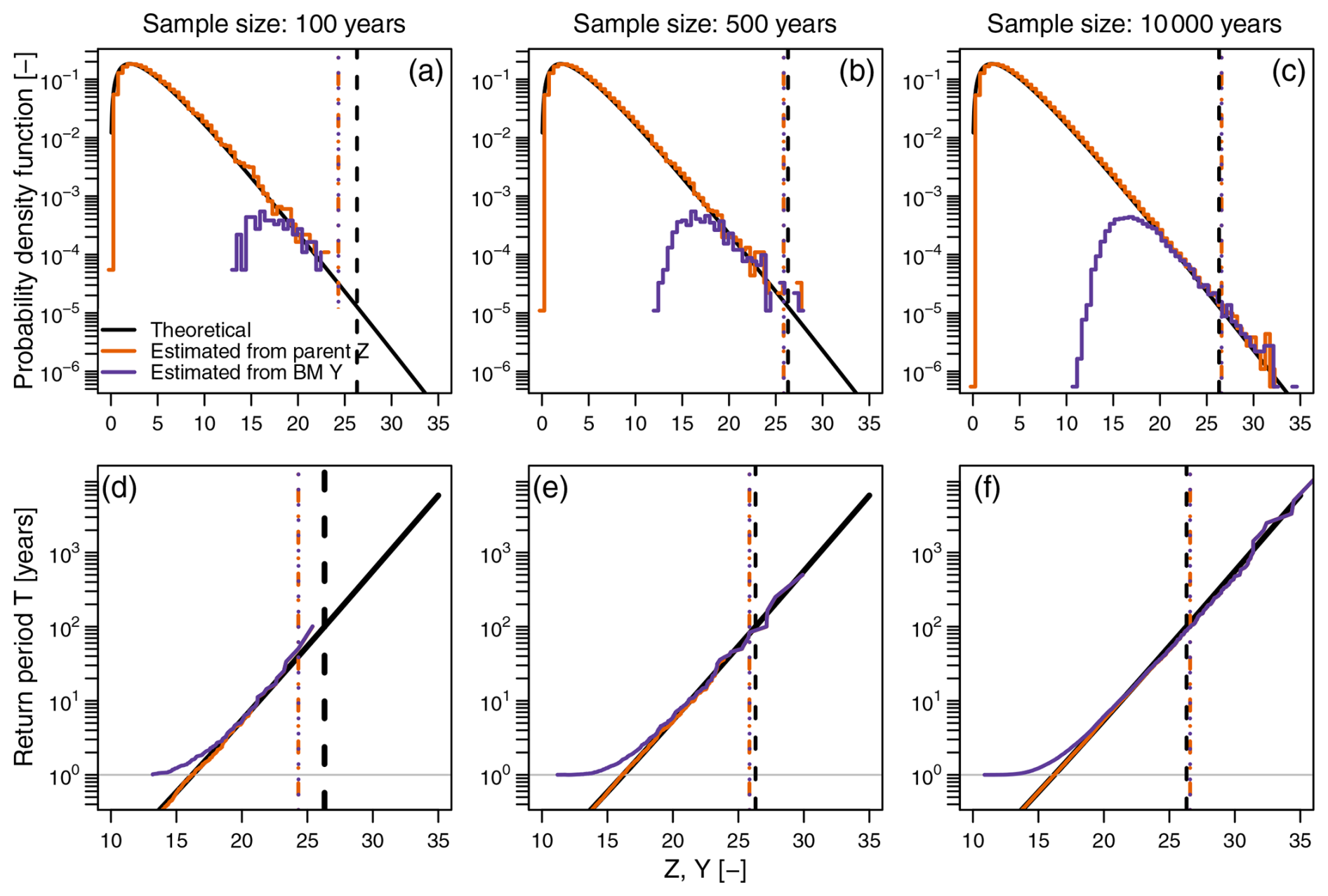
Figure 1 Probability density functions (a–c) and return level plots (return period vs. return level; d–f) of samples of varying size (365 × $\mathit{\{}\mathrm{100},\mathrm{500},\mathrm{10}\mathrm{000}\mathit{\}}$) and corresponding BM (with block size m=365) drawn from a gamma distribution. The diagrams show the relationship between the parent distribution and the distribution of BM, along with the convergence of the upper tails of the empirical distribution toward the theoretical counterparts. The abscissa of dashed vertical lines indicates the value of the theoretical 100-year return level (gray lines) and its estimates from samples of the parent process Z (blue lines) and the corresponding BM process Y (red lines).

For 𝒯 greater than ≅ 20 years, the upper tail of the empirical F_Y (f_Y) matches that of the empirical F_Z (f_Z). This matching and convergence to the upper tail of the theoretical F_Z (f_Z) improve as the sample size increases. This behavior is further stressed focusing on the 100-year return levels (vertical lines in Fig. 1). It should be noted that the discrepancies between F_Y and F_Z for 𝒯 < 20 years do not depend on the sample size. Instead, they are related to the different natures of the processes Y and Z, and their magnitude also depends on autocorrelation when data are correlated (see Sect 3.2 in Serinaldi et al., 2020b, for a theoretical discussion). Both distributions provide very close estimates of the 100-year return level for each sample size, and the accuracy obviously improves as the sample size increases. Moreover, Fig. 1 provides an intuitive (albeit very simplified) explanation of why EVT models of BM work when F_Z is not available and when EVT assumptions are fulfilled.

From Fig. 1, it is evident that we do not need any model for Y if we already have a model for the parent Z. Since 𝒩𝒜 distributions require the preliminary definition or fit of a model for F_Z, they have no practical usefulness as the preliminarily fitted F_Z already provides all the information required to make statements on both ordinary and extreme events or quantiles. In this respect, defining 𝒩𝒜 distributions from F_Z is only an unnecessary and redundant step, yielding only an approximation of the embedded F_Z. These issues are further discussed in the next section in a review of a real-world data analysis previously reported in the literature.

4.2 Re-analysis of sea level data

In this section, we further illustrate the foregoing concepts by re-analyzing two sea level time series already studied by Caruso and Marani (2022). These data refer to hourly sea level records from the tide gauge of Hornbæk (Denmark) and Newlyn (United Kingdom), spanning 122 years (1891–2012) and 102 years (1915–2016), respectively. Data are freely available from the University of Hawaii Sea Level Center (UHSLC) repository (Caldwell et al., 2015, http://uhslc.soest.hawaii.edu/data/?rq#uh745a/, last access: 23 August 2022). For the sake of consistency with the original work, we removed years with less than 6 months of water level observations and days with less than 24 h of data (see Caruso and Marani, 2022). This resulted in 120 and 100 years of data for the Hornbæk and Newlyn gauges, respectively. Moreover, time series are pre-processed by filtering out the time-varying mean sea level ($\mathrm{m}.\mathrm{s}.\mathrm{l}.$) computed using the average of daily levels for each calendar year. Thus, the filtered time series retain the contributions from astronomical tides and storm surges.

Daily maxima are used as the basis for extreme-value analysis, which is performed by means of three different approaches: (i) GEV distribution of AM, (ii) GP distribution of POTs, and (iii) GP-based MEV of peaks over a moderate threshold (i.e., the so-called ordinary events). These extreme-value models assume that the underlying process is a collection of independent random variables. Since sea levels are a typical example of an autocorrelated process, data are preliminarily declustered by selecting peaks that are separated by at least 30 d to obtain (approximately) independent samples. In more detail, Caruso and Marani (2022) adopted “a threshold lag of 30 d, which yielded the minimum estimation error under the MEVD approach”. Therefore, declustered data are used to extract AM and POT samples over optimal statistical thresholds (Bernardara et al., 2014). Caruso and Marani (2022) selected the GP threshold for POTs by studying the stability of the GP shape parameter (Coles, 2001, p. 83), while they chose the moderate threshold of GP distributions entering MEV “by testing different threshold values and evaluating the goodness of fit of the distribution using diagnostic graphical plots”.

Before presenting results of extreme-value analysis, it is worth noting the following:

1. The extraction of independent data from correlated samples is referred to as “physical declustering” (Bernardara et al., 2014). Its algorithms rely on the physical properties of the process of interest (e.g., the lifetime of the weather systems generating a storm over an area) and/or the properties of the occurrence process (e.g., statistics of the (inter-)arrival times of rainfall storms). In this respect, a threshold selection based on “the minimum estimation error under the MEVD approach” not only requires iterative fitting of MEV components but also contrasts with the rationale of physical declustering, whose algorithms should be unrelated to the subsequent analysis and models involved. In other words, physical declustering should guarantee only the independence of the extracted sample and not the goodness of fit of a specific model (GP, MEV, or anything else).

2. Goodness of fit concerns statistical optimization, which aims to set a threshold that guarantees the convergence or fit of the POT sample to an extreme-value model. For the GP model, such a threshold should provide “the best compromise between the convergence of [the POT distribution toward] a GP distribution (bias minimization) and the necessity to keep enough data for the estimation of its parameters (variance minimization)” (Bernardara et al., 2014). In the present case, such a statistical threshold should not be required as the physical threshold was already selected to yield “the minimum estimation error under the MEVD approach” (Caruso and Marani, 2022). In fact, for Hornbæk and Newlyn data sets, the thresholds used by Caruso and Marani (2022) (i.e., 40 and 250 cm, respectively) lead us to discard approximately only 13 % of the complete declustered sample. Therefore, for the sake of comparison, we applied MEV to both the original declustered data and their over-threshold sub-samples.

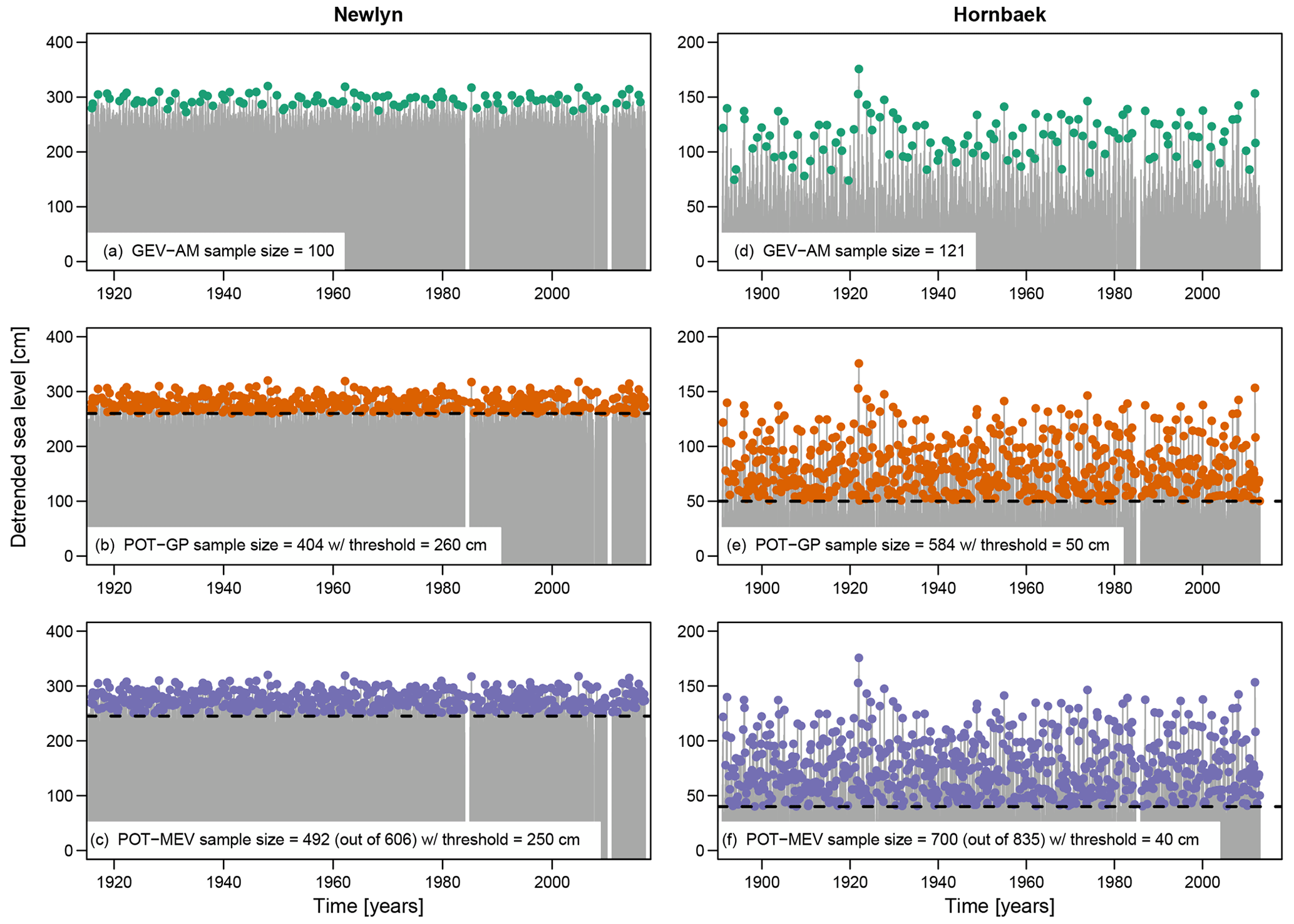
Figure 2 Detrended sea levels (gray line) for the gauging sites of Newlyn (UK) and Hornbæk (Denmark) and AM values for GEV analysis (a, d), POTs used for GP analysis (b, e), and over-threshold events used for fitting MEV and compound parent models (c, f). “Detrended” refers to sea level time series preliminarily filtered by removing the time-varying mean sea level.

For both data sets, Fig. 2 shows the time series of AM (Fig. 2a and d), POTs for GP (Fig. 2b and e), and POTs for MEV (Fig. 2c and f), along with the complete sample of daily maxima. Note that the sizes of POT samples are slightly different from those reported by Caruso and Marani (2022). This is likely due to the slightly different implementations of the declustering algorithm, which involves some technicalities such as the treatment of unavailable values.

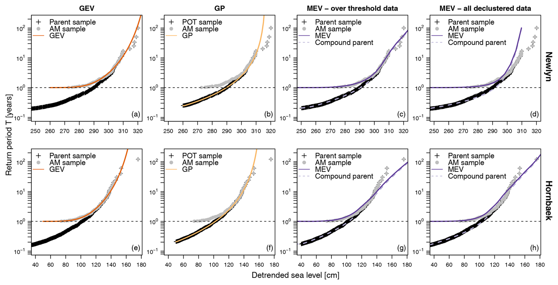
Figure 3 Return level diagrams (return period (in years) vs. return level) resulting from extreme-value analysis of Newlyn data (a–d) and Hornbæk data (e–h). All panels report empirical return level diagrams of AM as a common reference. Panels (a) and (e) report empirical return level diagrams of the parent sample of declustered data along with the theoretical return level diagram of the fitted GEV model. Panels (b) and (f) refer to POT sample and the corresponding GP model. Panels (c) and (g) and panels (d) and (h) show results for the MEV and compound parent distributions applied to the over-threshold data and complete declustered sample, respectively.

Figure 3 reports the results of extreme-value analysis in terms of return level plots. Figure 3a shows the empirical return level plot of the AM sample used to fit the GEV distribution and that of the corresponding declustered sample used to extract AM values. The values of the return period used to build these diagrams are estimated as $\mathcal{T}=\frac{\mathit{\mu }}{\mathrm{1}-F_n}$, where F_n is the empirical cdf of AM or the declustered sample, and μ is the average inter-arrival time between two observations of a (discrete-time) process of interest, i.e., μ=1 for AM and $\mathit{\mu }=\mathbb{E}[\mathrm{1}/L]$ for the complete declustered sample, where the random variable L denotes the varying number of events (or peaks) per year. Figure 3a and e are analogous to Fig. 1 and convey the same message but for real-world data; that is, the distribution of AM is only an approximation converging to the distribution of the parent sample for large quantiles (upper tail).

When using POT values over the threshold optimizing the GP fitting (Fig. 3b and f), we get a similar message: the distribution of AM is an approximation of the upper tail of the distribution of POTs, which plays a role similar to that of the parent sample in 𝒩𝒜 models of BM. In fact, the GP-based analysis of POTs does not require the subsequent derivation of the distribution of AM to make inferences regarding return levels as the return period (in years) of any quantile is computed as $\mathcal{T}=\frac{\widehat{\mathit{\mu }}}{\mathrm{1}-F_{\text{GP}}}$, where F_GP is the GP cdf, and $\widehat{\mathit{\mu }}$ is the estimate of the average inter-arrival time between two POT observations. Even though this remark can seem trivial, it plays a key role in understanding the redundancy of 𝒩𝒜 distributions.

MEV models require us to preliminarily fit a model for values above a moderate threshold (or all available independent declustered data), which is our parent distribution F_Z, and therefore derive the distribution of the annual maxima F_Y as a function of F_Z. Figure 3c, d, g, and h show the empirical cdf's of both the AM and parent sample, as well as their theoretical counterpart, i.e., the GP-based MEV model and the compound GP parent. As for GEV, the MEV distribution is only an approximation of the upper tail of the fitted compound parent. However, in this case, we already have a model for the parent process, and, therefore, we do not need any distribution of AM as the fitted compound F_Z already provides all the information required for inferential purposes. In other words, MEV cannot provide the correct probability of low or moderate quantiles (as with every extreme-value model of BM), and it cannot add any information compared to the corresponding fitted compound parent F_Z. Once F_Z is available, any other model of any sub-process (such as AM or POTs) is less informative or redundant, at most.

Figure 3c, d, g, and h also show that the claimed goodness of fit of MEV models is related to the fact that they are compound distributions rather than the fact that they are distributions of AM. In fact, MEV tails match those of the corresponding compound parent distributions. When we have a good compound model F_Z integrating (i.e., averaging) seasonal fluctuations and other forcing factors (such as different generating mechanisms of rainfall, storms, flood, or storm surges), the corresponding 𝒩𝒜 model is no longer needed as it can, at most, be as accurate as the corresponding compound F_Z.

The use of 𝒩𝒜 distributions is not even justified in making inferences regarding the return period and return levels. In fact, a compound F_Z can be used to compute return levels in the same way as one uses GP distributions, calculating the return period as $\mathcal{T}=\frac{\widehat{\mathit{\mu }}}{\mathrm{1}-F_Z}$, where $\widehat{\mathit{\mu }}$ is the estimate of the average inter-arrival time between two observations in the sample of values above a moderate threshold (as for the case in Fig. 3c and g) or in the complete sample of independent declustered data (as for the case in Fig. 3d and h). In general, F_Z does not require the derivation of the corresponding 𝒩𝒜 model for AM to make inferences with regard to the return period (expressed in years) in the same way as GP-based inference for POTs does not require the corresponding GEV model of AM.

5 Smoke and mirrors on the water extremes: a matter of compound distributions, neglected dependence, and misuse of multi-model ensemble averaging

The discussion in Sects. 3 and 4 was based on conceptual arguments, simplified numerical examples, and real-world data re-analysis with simple visual assessment. However, to be consistent with the scientific method, new models and methods should be validated or falsified against challenging and controlled conditions before being applied to real-world data coming from inherently unknown processes (Serinaldi et al., 2020a, 2022b). To this end, we set up three Monte Carlo experiments. The first experiment replicates and expands the numerical simulations reported by Marra et al. (2018) with the aim of providing independent validation and further evidence about the redundancy of 𝒩𝒜 models (here, MEV) when dealing with serially independent processes. The second experiment investigates the effect of autocorrelation on 𝒩𝒜-based analysis, evaluating the effectiveness of declustering algorithms based on threshold lags, as well as the use of βℬC models accounting for serial correlation without declustering. The third experiment replicates and expands some of the Monte Carlo simulations reported by Marani and Ignaccolo (2015) to support the introduction of MEV models. In this case, the aim is to explain the apparent discrepancies between the results in Marani and Ignaccolo (2015) and those in Marra et al. (2018).

5.1 Monte Carlo experiment 1: serially independent processes

The first experiment consists of simulating S=1000 time series of ordinary events mimicking 3, 5, 10, 20, and 50 years of records. Each year comprises l events drawn from a random variable L following a Gaussian distribution with a mean of ${\mathit{\mu }}_L\in \mathit{\{}\mathrm{10},\mathrm{50},\mathrm{100}\mathit{\}}$ and a standard deviation of σ_L = 0.3 μ_L. Marra et al. (2018) chose the range of μ_L and σ_L based on exploratory analysis of hourly rainfall data collected over the contiguous United States. Ordinary events are simulated from Weibull distributions with the shape parameter $\mathit{\kappa }\in \mathit{\{}\mathrm{0.8},\mathrm{1.25}\mathit{\}}$ and the scale parameter λ=1. The κ values represent the typical range of variability of the observed rainfall data studied by Marra et al. (2018), while a constant λ is chosen for easier interpretation of the results. The simulated time series are used to estimate the 100-year return levels. The reference 100-year return level is empirically obtained from 10⁵ years of simulated samples, and the performance of GEV, GP, and MEV is checked in terms of multiplicative bias:

$$\begin{array}{}\text{(8)}& B_k={\displaystyle \frac{{\widehat{x}}_k}{x_{\text{ref}}}},\end{array}$$

where ${\widehat{x}}_k$ is the estimate of the target statistics (here, 100-year return level) for the kth Monte Carlo simulation (with $k=\mathrm{1},\mathrm{\dots },S$), and x_ref is the reference (true) value.

We note that the use of a Gaussian distribution with infinite support can generate a physically inconsistent negative number of events in some years. Moreover, simulating integer values from a continuous distribution requires rounding off. In these cases, more appropriate models for discrete random variables defined in [0,∞), such as binomial, beta-binomial, Poisson, or geometric, should be used. The reference 100-year return level can be computed as the $(\mathrm{1}-\frac{\mathrm{1}}{\mathrm{100}})\cdot$ 100 % quantile of the empirical cdf of AM or the $(\mathrm{1}-\frac{\widehat{\mathit{\mu }}}{\mathrm{100}})\cdot$ 100 % quantile of the empirical cdf of the complete time series of ordinary events, where $\widehat{\mathit{\mu }}$ is the estimate of the average inter-arrival time (in years) between two ordinary events. For large samples, the former estimate converges to the latter for 𝒯 values greater than a few years (e.g., 3–5 years for independent data; see Fig. 1) or much more for serially dependent processes (see Sect 3.2 in Serinaldi et al., 2020b). In any case, the most accurate estimate of the 𝒯-year return level for every value of 𝒯 is given by the distribution F_Z of the parent process, thus making the derivation of the distribution F_Y of AM redundant if the latter requires the preliminary definition of the former.

Results are reported as diagrams of the 5 %, 50 %, and 95 % quantiles of multiplicative bias versus the number of years. As expected, Fig. 4 is in perfect agreement with Fig. 7 in Marra et al. (2018) and leads to the same overall conclusions: MEV exhibits positive bias compared to GEV and GP but smaller variance. However, Fig. 4 provides an additional result concerning the performance of the compound parent distribution corresponding to MEV and shows that both models yield almost identical results apart from unavoidable sampling fluctuations in the estimation of the 5 % and 95 % quantiles based on 1000 simulated values of bias B. As discussed in Sects. 3 and 4, MEV distributions (or, more generally, 𝒩𝒜 distributions) do not add any information with respect to the parent distribution appearing in MEV formulas. Therefore, once a distribution is selected to describe the ordinary events (here, Weibull), its compound version is enough to make statements regarding any quantile, providing more information than the derived compound 𝒩𝒜 models, which approximate only the upper tail of the (embedded) parent distribution.

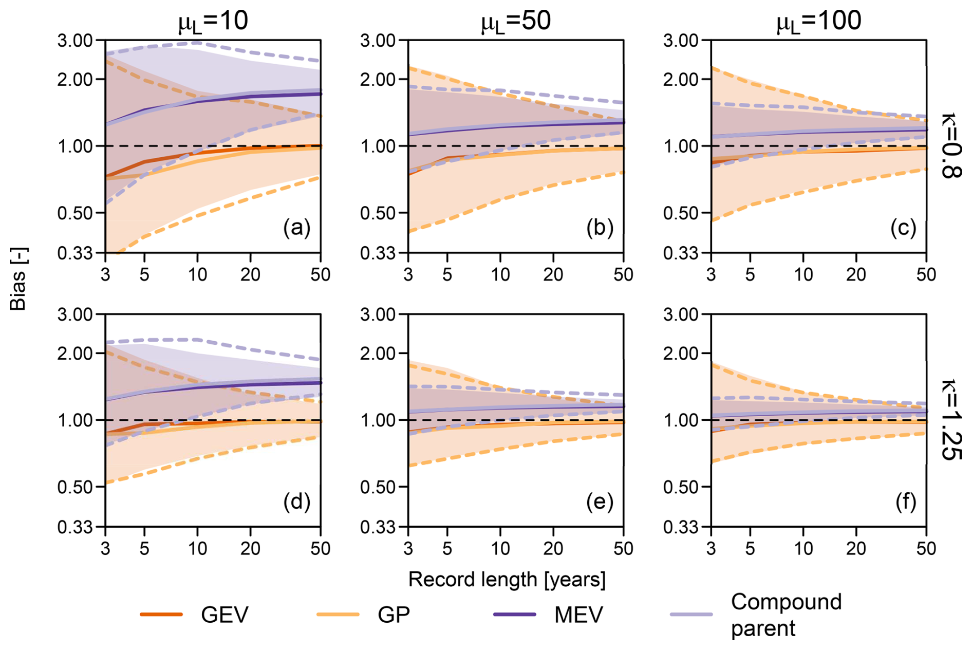
Figure 4 Multiplicative bias for the 100-year return levels obtained from 1000 synthetic samples of varying record length (i.e., number of blocks or years) and with a varying number of ordinary events per block or year (10, 50, and 100) drawn from Weibull distribution with shape parameters κ=0.8 (a–c) and 1.25 (d–f). The reference 100-year return levels are empirically obtained from a 10⁵-year record. Solid lines represent the median bias, while shaded areas (for GEV and MEV) and dashed lines (for GP and Compound parent) represent the 95 % Monte Carlo confidence intervals.

5.2 Monte Carlo experiment 2: serially dependent processes

This Monte Carlo experiment is designed to study the effect of autocorrelation on 𝒩𝒜-based inference. Time series of ordinary events mimicking 3, 5, 10, 20, and 50 years of daily records (i.e., 365 records per year) are simulated S = 1000 times to estimate 100-year return levels. The marginal distributions are the same as those used in the first experiment, i.e., Weibull with shape parameter $\mathit{\kappa }\in \mathit{\{}\mathrm{0.8},\mathrm{1.25}\mathit{\}}$ and scale parameter λ=1. Autocorrelation is modeled by a first-order autoregressive (AR(1)) process with parameter ${\mathit{\rho }}_{\mathrm{1}}\in \mathit{\{}\mathrm{0.3},\mathrm{0.6},\mathrm{0.9}\mathit{\}}$, corresponding to weak, moderate, and relatively high autocorrelation. Weibull-AR(1) time series are generated by the CoSMoS framework, which enables the simulation of correlated processes with the desired marginal distribution and ACF (Papalexiou, 2018, 2022; Papalexiou and Serinaldi, 2020; Papalexiou et al., 2021, 2023).

Extreme-value analysis is performed by GEV for AM, GP for POTs of preliminarily declustered data, Weibull-based MEV for declustered data, and Weibull-based βℬC for the complete time series. Declustering is based on time lag, selecting the first lag τ₀ such that the empirical ACF becomes smaller than twice the 99 % quantile of the sampling distribution of the ACF values under independence. Although this approach is slightly different from that used by Marra et al. (2018), the rationale is the same, and it yields τ₀ values that guarantee sufficiently long inter-arrival times, as well as a suitable number of events per block for the considered AR(1) ACFs and sample sizes. Subsets of ordinary events used for MEV analysis are then defined as peaks separated by time intervals ≥τ₀. POTs for GP analysis are extracted from these subsets, while AM for GEV analysis are selected from the original sample, assuming their inter-annual independence. Of course, βℬC analysis uses the complete data set and does not require any preliminary declustering procedure as it explicitly accounts for autocorrelation.

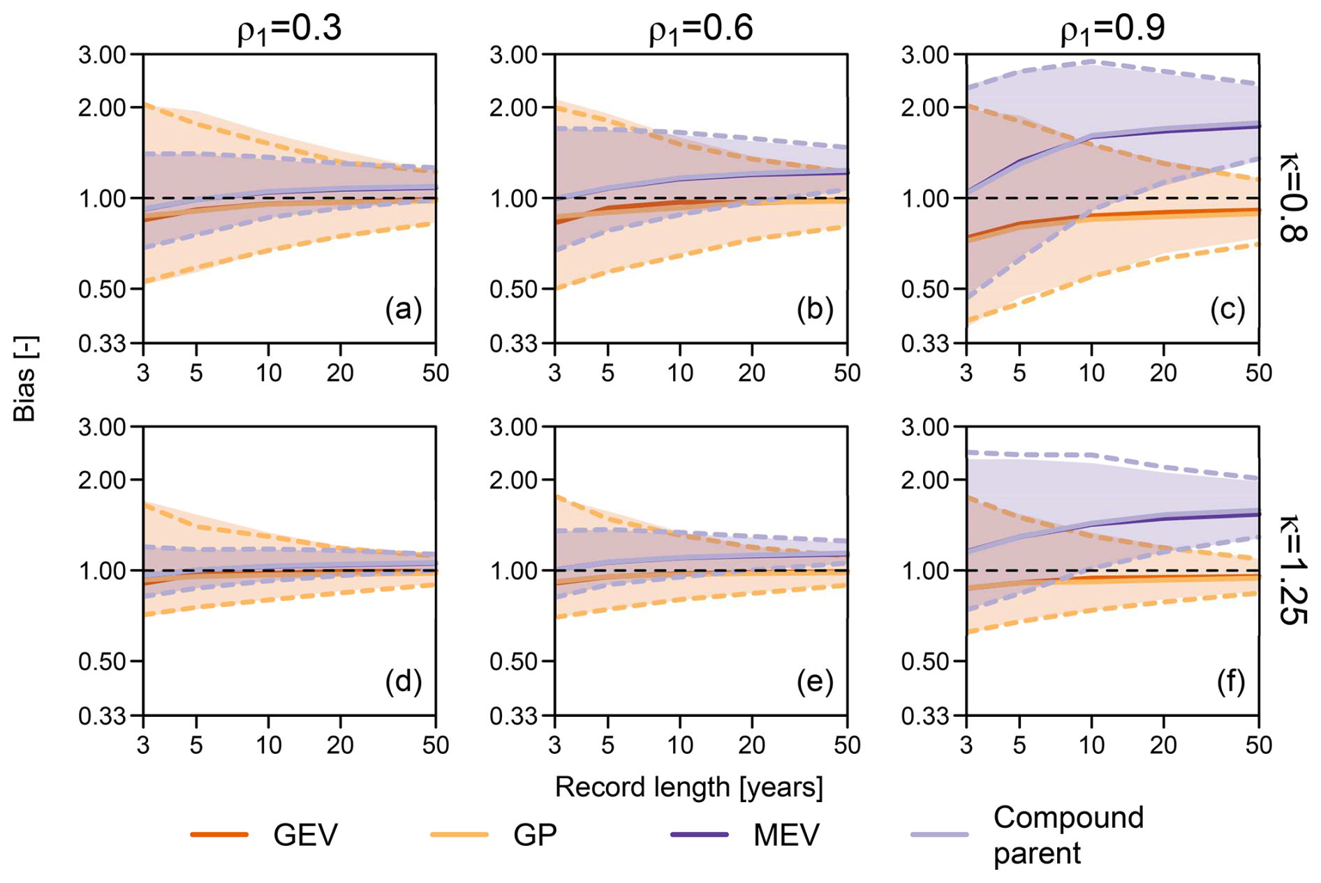
Figure 5 Multiplicative bias for the 100-year return levels obtained from 1000 synthetic samples of varying record length (i.e., number of blocks or years) from the Weibull-AR(1) process, with Weibull shape parameters κ=0.8 (a–c) and 1.25 (d–f) and AR(1) parameter $\mathit{\rho }\in \mathit{\{}\mathrm{0.3},\mathrm{0.6},\mathrm{0.9}\mathit{\}}$. The reference 100-year return levels are empirically obtained from a 10⁵-year record. Solid lines represent the median bias, while shaded areas (for GEV and MEV) and dashed lines (for GP and compound parent) represent the 95 % Monte Carlo confidence intervals. MEV and compound parent distributions are fitted to preliminarily declustered data.

Figure 5 compares the results of the GEV, GP, and MEV analyses. For ρ₁=0.3, values of bias B are similar to those obtained for the previous experiment in Sect. 5.1, with μ_L=100 (Fig. 4). This is expected as low values of ρ₁ correspond to rapidly decreasing ACF and, therefore, τ₀≅ 2–3 time steps, corresponding to sample sizes of ordinary events between about 120 and 180. For ρ₁=0.6 and 0.9, τ₀ increases to 4–6 and 15–30 time steps, respectively, corresponding to sample sizes of 60–90 and 12–24 ordinary events. The progressively reduced sample size increases MEV uncertainty, which becomes similar to that of GEV and GP models. More importantly, MEV bias dramatically increases with ρ₁ and the number of years (blocks). The effect of ρ₁ is easy to interpret in terms of reduced sample size resulting from declustering with larger τ₀. On the other hand, the effect of the number of years could appear to be counterintuitive as one would expect more accuracy when a larger number of years is available.

Marra et al. (2018) ascribe this behavior “to uncertain estimation of the weight of the tail of the ordinary events distribution when few data points are used for the fit”. However, this would not be sufficient to explain why the smallest bias corresponds to small numbers of available years and, thus, to overall smaller samples. The actual issue is the combination of the (average) number of intra-block peaks (or intra-block sample sizes – here, l or μ_L), the number of blocks (here, the number of years n_Y), and the compounding procedure characterizing MEV.

For fixed n_Y, a small intra-block sample size l results in great variability in the Weibull parameters estimated in each block, which, in turn, results in heavier tails of compound distributions. As l increases, the inter-block variability of Weibull parameters decreases, and the compound distribution resulting from averaging a set of similar Weibull distributions becomes closer and closer to the theoretical Weibull used to simulate. In other words, the compounding mechanism works better in those cases in which it is less required, i.e., when the inter-block variability is small and when model averaging (of very similar models fitted on each block) is less justified and useful. On the other hand, when model averaging could be more justified, i.e., when there is substantial uncertainty in the sampling parameters, the dispersion of the sampling distribution of parameters is greater, and the tail of the resulting compound distribution is heavier, with a shape departing from that of the (true) theoretical distribution.

For given μ_L, when the number of years n_Y is small, compound 𝒩𝒜 models average a small number of components $F_j^{l_j}$, with $j=\mathrm{1},\mathrm{\dots },n_Y$ (e.g., we have three components for n_Y = 3 years). In a Monte Carlo experiment, averaging a few heterogeneous components results in a set of heterogeneous compound distributions whose differences tend to compensate for each other, on average. Therefore, the Monte Carlo ensembles of compound distributions exhibit high variability and small bias. As n_Y increases, the number of averaging components $F_j^{l_j}$ increases, providing a more accurate picture of the inter-block variability that is incorporated into the compound distributions. This results in Monte Carlo ensembles of compound distributions with more homogeneous and systematically heavier tails than those of the compound models resulting from small n_Y. Therefore, the Monte Carlo ensemble exhibits lower variance and higher bias as n_Y increases for a given μ_L.

As for Fig. 4, Fig. 5 also reports results for the compound distribution of ordinary events, which are almost indistinguishable from those of MEV analysis. Overall, Fig. 5 further confirms the redundancy of MEV models (and, more generally, 𝒩𝒜 models) once we have a compound parent distribution, which has to be estimated in any case to derive 𝒩𝒜 distributions. Moreover, uncorrelated ordinary events resulting from declustering procedures do not guarantee convergence of compound distributions (MEV or parent) to the true distribution. In fact, the bias is generally much larger than that of GEV and GP estimates, although the intra-block sample size is generally much larger than that of AM and POTs, and the compound distributions have a much larger number of parameters (from 6 to 100, resulting from the two-parameter Weibull fitted to 1-year blocks over 3 to 50 years).

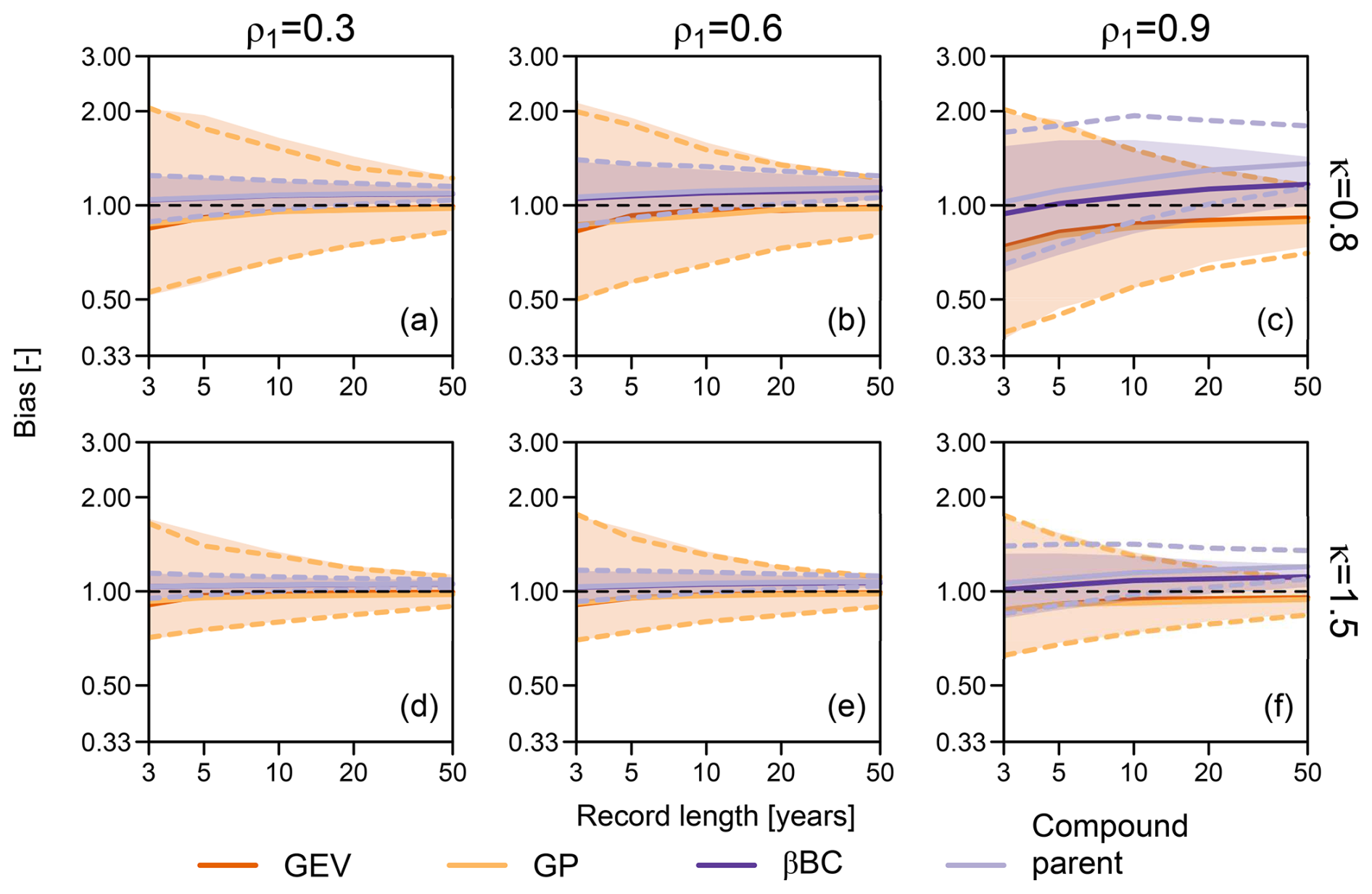
Figure 6 Multiplicative bias for the 100-year return levels obtained from 1000 synthetic samples of varying record length (i.e., number of blocks or years) from the Weibull-AR(1) process, with Weibull shape parameters κ=0.8 (a–c) and 1.25 (d–f) and AR(1) parameter $\mathit{\rho }\in \mathit{\{}\mathrm{0.3},\mathrm{0.6},\mathrm{0.9}\mathit{\}}$. The reference 100-year return levels are empirically obtained from a 10⁵-year record. Solid lines represent the median bias, while shaded areas (for GEV and MEV) and dashed lines (for GP and compound parent) represent the 95 % Monte Carlo confidence intervals. βℬC and compound parent distributions are fitted to complete autocorrelated time series.

Figure 6 compares the results of the GEV and GP analyses with those of βℬC and compound parent models. Since βℬC models (and the corresponding compound parent) use the complete time series instead of declustered data, uncertainty and bias are smaller than those of MEV models (and the corresponding compound parent). Therefore, while time lag declustering seems to yield apparently independent events, the resulting data sets do not provide a faithful description of the upper tail of the true generating process; that is, MEV models do no make suitable use of these declustered samples. Declustering has negative effects independently of the intensity of autocorrelation. Of course, larger bias and uncertainty correspond to higher ρ₁ values in both MEV and βℬC analyses. In fact, MEV is affected by significant decreases in sample size due to declustering, while βℬC suffers from underestimation of ACF, which requires large sample sizes to be reliably estimated (see, e.g., Koutsoyiannis and Montanari, 2007; Serinaldi and Kilsby, 2016a). It is worth noting that the GEV and GP results are rather insensitive to autocorrelation. This is expected as the underlying joint dependence structure of AR(1) processes is a Gaussian copula, which is characterized by asymptotic tail independence and is therefore complaint with EVT assumptions. Similarly to Fig. 4 and 5, Fig. 6 shows that the βℬC model and the corresponding compound parent match (apart from discrepancies due to the issues mentioned above), confirming the redundancy of 𝒩𝒜 models.

5.3 Monte Carlo experiment 3: reviewing simulations of Marani and Ignaccolo (2015)

Figure 4 shows that MEV and its compound parent distribution yield a median multiplicative bias B_M≅1.25 for 100-year return levels estimated from n_Y = 50 years (blocks) of data drawn from Weibull distributions with the shape parameter κ=0.8 and an average number of events per block of ${\mathit{\mu }}_L\in \mathit{\{}\mathrm{50},\mathrm{100}\mathit{\}}$. On the other hand, B_M≅1.0 for GEV and GP distributions. For a similar setup (i.e., n_Y=50, κ=0.82, and ${\mathit{\mu }}_L\in \mathit{\{}\mathrm{30},\mathrm{100}\mathit{\}}$), Marani and Ignaccolo (2015) reported probability plots (probability vs. quantiles) and relative error:

$$\begin{array}{}\text{(9)}& R_k={\displaystyle \frac{{\widehat{x}}_k-x_{\text{ref}}}{x_{\text{ref}}}},\end{array}$$

where ${\widehat{x}}_k$ is the estimate of the target statistics for the kth Monte Carlo simulation (with $k=\mathrm{1},\mathrm{\dots },S$), and x_ref is the reference (true) value. They found that MEV is almost unbiased, with an average relative error of $\stackrel{\mathrm{‾}}{R}=\frac{\sum R_k}{S}\cong \mathrm{0}$, while GEV exhibits bias, with $\stackrel{\mathrm{‾}}{R}\cong$ 5 % and ≅ 30 % for the 100- and 1000-year return levels, respectively. On the other hand, for the 100-year return level, simulations in Sect. 5.1 (reproducing those of Marra et al., 2018) yield $\stackrel{\mathrm{‾}}{R}\cong$ 25 % for MEV and $\stackrel{\mathrm{‾}}{R}\cong \mathrm{0}$ for GEV. Therefore, we re-run Monte Carlo simulations described by Marani and Ignaccolo (2015) to understand the reason for such a disagreement. We anticipate that the foregoing discrepancies depend on the misuse of methods used to summarize multi-model ensembles. Thus, before describing Monte Carlo experiments and their outcome, we need to recall some theoretical concepts that are required to correctly interpret numerical results.

5.3.1 Summarizing multi-model ensembles: some overlooked concepts

Monte Carlo simulations are usually used to study the uncertainty affecting estimates based on finite-sized samples (that provide incomplete information about the underlying process) or to approximate population distributions (or statistics) when mathematical closed-form expressions are not available. Examples of these applications are the experiments reported in Sect. 5.1 and 5.2.

In all cases, the primary output of Monte Carlo simulations is a set of parameters identifying a set of models (multi-model ensemble) that is then used to estimate the target statistics of interest. For example, simulations of S finite-sized samples in Sect. 5.1 and 5.2 are used to fit a set of S GEV distributions. These are then used to calculate a set of S 100-year return levels, which are eventually used to build confidence intervals summarizing sampling uncertainty.

However, a multi-model ensemble can be summarized in many different fashions to obtain a representative point estimate of a statistic of interest (e.g., Renard et al., 2013; Fawcett and Walshaw, 2016; Fawcett and Green, 2018). Let S be the number of Monte Carlo replications; let F(z|θ_k) (with $k=\mathrm{1},\mathrm{\dots },S$) be the kth member of the Monte Carlo multi-model ensemble (e.g., the kth Weibull distribution fitted to the kth simulated sample); let z_p be a target quantile with a non-exceedance probability p; and let us define the quantile function as the inverse of the cdf, $Q=F^{-\mathrm{1}}$. A representative point estimate of z_p can be, for instance, the mode of the S quantiles $z_{p,k}=Q\left(p\right|{\mathit{\theta }}_k)=F^{-\mathrm{1}}(p\left|{\mathit{\theta }}_k\right)$.

More popular point estimates of z_p (or whatever statistics) rely on the definition of so-called predictive distributions and predictive quantile functions. The sampling predictive cdf reads as

$$\begin{array}{}\text{(10)}& \begin{array}{rl}\stackrel{\mathrm{‾}}{F}\left(z\right):=& {\displaystyle \frac{\mathrm{1}}{S}}\sum _{k=\mathrm{1}}^{S}F\left(z\right|{\mathit{\theta }}_k)\\ \cong & {\mathbb{E}}_{{\mathrm{\Omega }}_{\mathit{\theta }}}\left[F\right(z\left|\mathbf{\Theta }\right)],\end{array}\end{array}$$

and the corresponding quantile with a specified non-exceedance probability p is given by

$$\begin{array}{}\text{(11)}& \begin{array}{rl}{z}_{p,\stackrel{\mathrm{‾}}{F}}=& \left\{z:{\displaystyle \frac{\mathrm{1}}{S}}\sum _{k=\mathrm{1}}^{S}F\left(z\right|{\mathit{\theta }}_k)=\stackrel{\mathrm{‾}}{F}(z)=p\right\}\\ =& {\stackrel{\mathrm{‾}}{F}}^{-\mathrm{1}}\left(p\right).\end{array}\end{array}$$

The sampling predictive quantile function reads as

$$\begin{array}{}\text{(12)}& \begin{array}{rl}\stackrel{\mathrm{‾}}{Q}\left(p\right):=& {\displaystyle \frac{\mathrm{1}}{S}}\sum _{k=\mathrm{1}}^{S}Q\left(p\right|{\mathit{\theta }}_k)\\ \cong & {\mathbb{E}}_{{\mathrm{\Omega }}_{\mathit{\theta }}}\left[Q\right(p\left|\mathbf{\Theta }\right)]={\mathbb{E}}_{{\mathrm{\Omega }}_{\mathit{\theta }}}[F^{-\mathrm{1}}\left(p\right|\mathbf{\Theta }\left)\right],\end{array}\end{array}$$

resulting in predictive quantile estimates of

$$\begin{array}{}\text{(13)}& \begin{array}{rl}{z}_{p,\stackrel{\mathrm{‾}}{Q}}=& {\displaystyle \frac{\mathrm{1}}{S}}\sum _{k=\mathrm{1}}^S{F}^{-\mathrm{1}}\left(p\right|{\mathit{\theta }}_k)\\ =& \stackrel{\mathrm{‾}}{F^{-\mathrm{1}}\left(p\right)}.\end{array}\end{array}$$

Let us denote the empirical cdf and quantile function of the S sampled quantiles z_p,k as F_S and Q_S, respectively. Recalling that the distribution of z_p can be approximated by the distribution of order statistics and that the latter is described by a generalized beta distribution (see Eq. 1, as well as Eugene et al., 2002; Tahir and Cordeiro, 2016), we can write $F_S\left(z_p\right)\cong F_{\mathit{\beta }}\left(F\right(z\left)\right|p{S}^{\prime },(\mathrm{1}-p)S^{\prime })$, where $S^{\prime }=S+\mathrm{1}$. Therefore, the foregoing z_p estimators can be complemented by the median estimator, defined as

$$\begin{array}{}\text{(14)}& \begin{array}{rl}{z}_{p,\mathrm{M}}=& \left\{z:\mathbb{P}[Z_{p,k}\le z]=F_S\left(z_p\right)=\mathrm{0.5}\right\}\\ =& F_S^{-\mathrm{1}}\left(\mathrm{0.5}\right)\cong F^{-\mathrm{1}}\left(F_{\mathit{\beta }}^{-\mathrm{1}}\left(\mathrm{0.5}\right|p{S}^{\prime },(\mathrm{1}-p)S^{\prime })\right).\end{array}\end{array}$$

Similarly, we can also define the median probability of a fixed quantile z_p from an ensemble of cdf's as follows:

$$\begin{array}{}\text{(15)}& \begin{array}{rl}{p}_{\mathrm{M}}=& \left\{p:Q_S\left(\mathrm{0.5}\right)=z_p\right\}\\ =& \left\{p:F_S\left(z_p\right)=\mathrm{0.5}\right\}\\ \cong & \left\{p:F_{\mathit{\beta }}\left(F\right(z_p\left)\right|p{S}^{\prime },(\mathrm{1}-p)S^{\prime })=\mathrm{0.5}\right\}.\end{array}\end{array}$$

The foregoing formulas indicate that the three z_p estimators obviously represent different quantities. Focusing on $z_{p,\stackrel{\mathrm{‾}}{F}}$ and $z_{p,\stackrel{\mathrm{‾}}{Q}}$ and comparing Eqs. (11) and (13), we have it that

$$\begin{array}{}\text{(16)}& {\stackrel{\mathrm{‾}}{F}}^{-\mathrm{1}}\left(p\right)\ne \stackrel{\mathrm{‾}}{F^{-\mathrm{1}}\left(p\right)}.\end{array}$$

Equation (16) is the sampling counterpart of $Q\left(\mathbb{E}\right[F\left(Z_p\right)\left]\right)\ne \mathbb{E}\left[Q\right(F\left(Z_p\right)\left)\right]\equiv \mathbb{E}\left[Z_p\right]$, which, in turn, follows from the well-known general inequality

$$\begin{array}{}\text{(17)}& \mathbb{E}\left[F\right(Z\left)\right]\ne F\left(\mathbb{E}\right[Z\left]\right),\end{array}$$

stating that the distribution of the expected value of Z is different from the expected distribution of Z. In fact, since F is commonly a nonlinear transformation of Z (as well as of the parameters θ), it hinders the interchangeability of the (linear) expectation operator 𝔼. In passing, such an inequality also partly caused a long “querelle” (controversy) with regard to plotting position formulas (see, e.g., Makkonen, 2008; Cook, 2012; Makkonen et al., 2013).

On the other hand, z_p,M is the only estimator that guarantees the identity between the z_p estimates obtained from ensembles of Q or F functions. This property depends on the fact that the median (as well as every quantile) is a rank-based (central-tendency) index, and ranking is a transformation that does not depend on absolute values and therefore passes unaffected trough nonlinear monotonic functions such as Q and F. This means that the median parameters θ_M correspond to z_p,M and p_M. This property does not hold for the expectation operator 𝔼. In fact, generally, $F\left(z_p\right|{\mathbb{E}}_{{\mathrm{\Omega }}_{\mathit{\theta }}}\left[\mathbf{\Theta }\right])\ne {\mathbb{E}}_{{\mathrm{\Omega }}_{\mathit{\theta }}}[F\left(z_p\right|\mathbf{\Theta }\left)\right]$.

The foregoing concepts and properties play a key role in the correct interpretation of the results reported in the next section.

5.3.2 Numerical simulations: the consequences of overlooking theory

Marani and Ignaccolo (2015) supported the introduction of MEV by means of five Monte Carlo experiments (referred to as cases “A”, “B”, “C”, “A2”, and “B2”), comparing the accuracy of MEV to that of standard asymptotic models of BM (i.e., Gumbel and GEV distributions). For the cases B and B2, Marani and Ignaccolo (2015) did not provide enough information to enable their replication. Therefore, we focused on cases A, C, and A2, which are sufficient to support our discussion. Case A consists of simulating S=1000 samples from a Weibull distribution with a scale parameter equal to 7.3, a shape parameter of κ=0.82, a number of blocks (years) of n_Y=50, and a number of events per block (here, wet days per year) of l=100. Case C is similar to A, with the only difference being that the number of events per block is drawn from a uniform distribution 𝒰(21,50). The setup of case A2 is similar to that of A; however, it explores the effect of varying l from 10 to 200 by steps of 10 events per block. Therefore, Gumbel, GEV, and MEV distributions of BM are fitted to each of the S samples. For the cases A and C, the accuracy of the three models is assessed by comparing “the ensemble average distributions, ζ_MEV(y), ζ_GEV(y), ζ_GUM(y) as the means of the distributions of Y computed over the 1000 synthetic time series” (Marani and Ignaccolo, 2015). For the case A2, the three models are evaluated in terms of the average relative error $\stackrel{\mathrm{‾}}{R}$ of the estimates of the 100- and 1000-year return levels. The reference (true) return levels are empirically obtained from 10⁶ years of simulated samples.

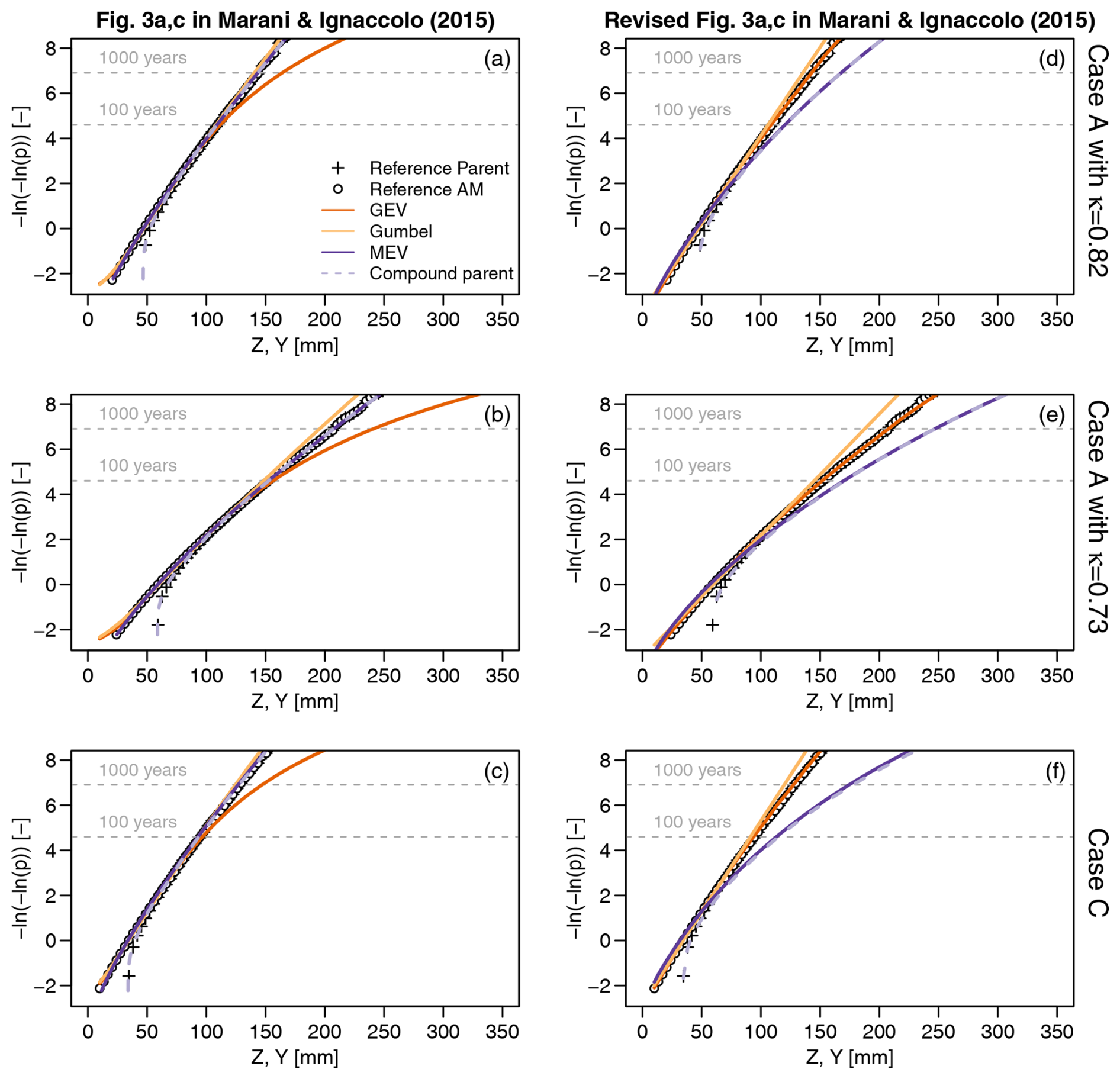
Figure 7 Probability plots (probability vs. quantile) showing different models for AM Y resulting from the Monte Carlo experiments denoted as cases A (a, b, d, e) and C (c, f) (see main text for details about the simulation setup). Panels (a–c) reproduce results reported in Marani and Ignaccolo (2015, Fig. 3a and c), while panels (d–f) show the revised version with corrections accounting for inconsistencies in the calculation of compound quantiles and the misuse of multi-model ensemble averaging.

Figure 7a–c reproduce Fig. 3a and c in Marani and Ignaccolo (2015). For the case A, we used both κ=0.82 and 0.73 as the original parameterization cannot reproduce the results of Fig. 3a in Marani and Ignaccolo (2015). In fact, analyzing the original Fig. 3a, the reference 100- and 1000-year return levels should be close to 150 and 210, respectively, while κ=0.82 yields values close to 109 and 143, which, in turn, are consistent with case C. Therefore, we used κ=0.73 to obtain a figure that is as close as possible to the original one. Nonetheless, the exact value of κ is inconsequential in the following discussion, and we use both κ=0.82 and 0.73 for completeness.

The key aspects in Fig. 7a–c are (i) the perfect match of MEV and its compound parent, confirming the redundancy of 𝒩𝒜 models when their parents are already known, and (ii) the accuracy of MEV and its compound parent against the prominent bias of GEV, which is in contrast to results reported by Marra et al. (2018) and in the previous sections. The reason for such a discrepancy is that Fig. 7a–c (and Fig. 3a in Marani and Ignaccolo, 2015) do not show what they are supposed to do, thus making the comparison unfair and misleading. In fact, contrarily to the description in Marani and Ignaccolo (2015), the MEV curves in Fig. 7a–c do not refer to the predictive MEV obtained by averaging S MEV distributions according to Eqs. (10) and (11). Instead, recalling that MEV is itself a predictive distribution (i.e., the average of multiple components $F_j^{l_j}$, with $j=\mathrm{1},\mathrm{\dots },n_Y$; see Sect. 2), MEV curves in Fig. 7a–c refer to the predictive version (averaged over S samples) of MEV quantile functions, which are predictive quantile functions themselves resulting from averaging over n_Y samples.

In other words, Fig. 7a–c report the pairs $(z_{p,\stackrel{\mathrm{‾}}{Q}},p)$ instead of the claimed $(z_{p,\stackrel{\mathrm{‾}}{F}},\stackrel{\mathrm{‾}}{F})$, and these pairs differ from each other (see Sect. 5.3.1). In more detail, $z_{p,\stackrel{\mathrm{‾}}{Q}}\cong {\mathbb{E}}_S\left[{\mathbb{E}}_{{\mathrm{\Omega }}_{{\mathit{\theta }}_S}}\right[{F_{\text{WEI}}^l}^{-\mathrm{1}}\left(p\right|{\mathbf{\Theta }}_S\left)\right]]$, while the figure should show $z_{p,\stackrel{\mathrm{‾}}{F}}$ obtained by inverting $\stackrel{\mathrm{‾}}{F}\cong {\mathbb{E}}_S\left[F_{\text{MEV}}\right]={\mathbb{E}}_S\left[{\mathbb{E}}_{{\mathrm{\Omega }}_{{\mathit{\theta }}_S}}\right[F_{\text{WEI}}^l\left(z_p\right|{\mathbf{\Theta }}_S\left)\right]]$.

On the other hand, Fig. 7a–c (and Fig. 3a and c in Marani and Ignaccolo, 2015) correctly show the predictive distributions of Gumbel and GEV. However, this hinders a fair comparison. In fact, EVT states that the asymptotic model of BM is a GEV distribution (under suitable conditions) and not the compound version of GEV resulting from averaging S GEV models. Such a compound GEV distribution always has a larger variance and heavier tails than its classical GEV counterpart (see Sect. 6). Therefore, to be consistent with EVT, the ensemble of GEV and Gumbel distributions should be summarized using a transformation, such as the median, that retains the expected GEV or Gumbel shape. Figure 7d–f show the median GEV and Gumbel distributions (resulting from Eq. 15), along with the actual predictive MEV (as it should be). Results in Fig. 7d–f are fully consistent with those reported by Marra et al. (2018) and in Sect. 5.1 and 5.2, confirming the low bias of asymptotic models and the natural tendency of compound distributions to exhibit heavier tails than their components and their generating processes. Moreover, the perfect agreement of the upper tail of MEV and that of the compound parent distributions in Fig. 7d–f further confirms (if still needed after many examples) the redundancy of 𝒩𝒜 models once their parent distributions are defined.

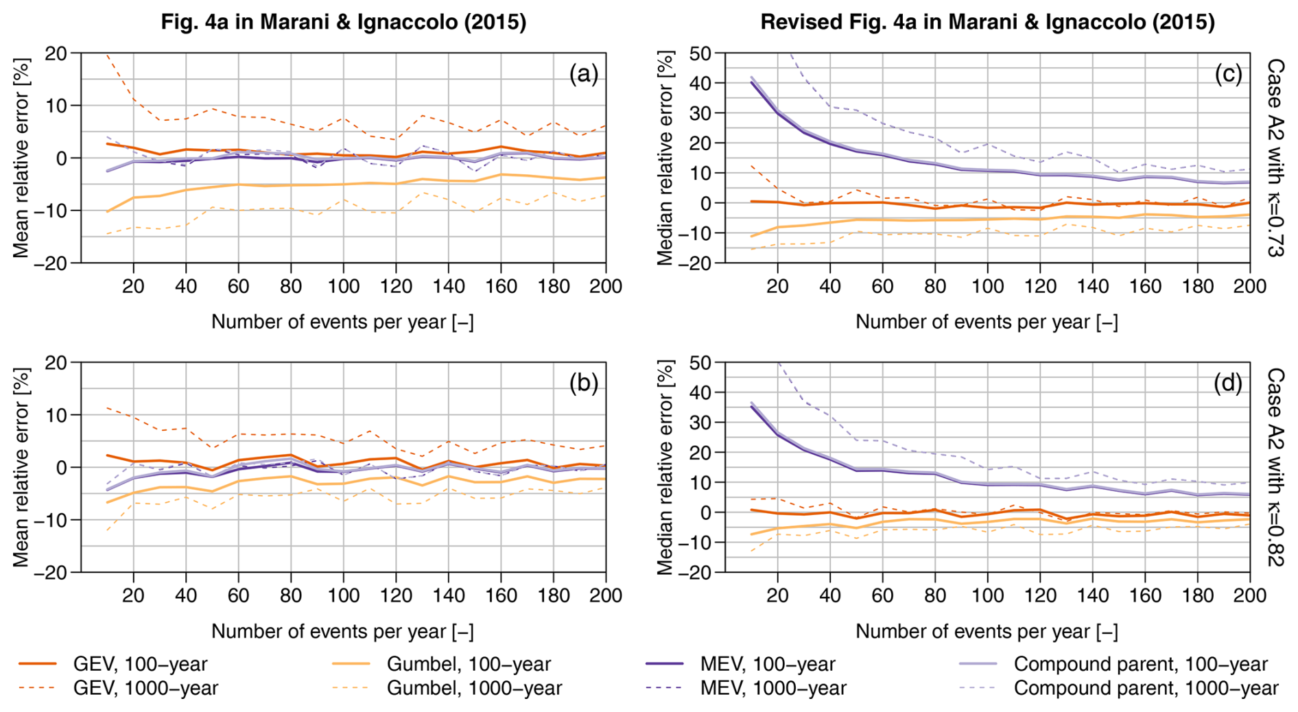
Figure 8 Relative errors for 100- and 1000-year return levels resulting from the Monte Carlo experiment denoted as case A2 (see main text for details about the simulation setup). Panels (a) and (b) reproduce results reported in Marani and Ignaccolo (2015, Fig. 4a) for $\mathit{\kappa }\in \mathit{\{}\mathrm{0.73},\mathrm{0.82}\mathit{\}}$, while panels (c) and (d) show the revised version with corrections accounting for inconsistencies in the calculation of compound quantiles and the misuse of multi-model ensemble averaging.

Similar remarks hold for the case A2. Results in Fig. 8a and b are close to those reported by Marani and Ignaccolo (2015) in their Fig. 4a, with MEV showing $\stackrel{\mathrm{‾}}{R}\cong \mathrm{0}$ for both the 100- and 1000-year quantiles and with GEV showing $\stackrel{\mathrm{‾}}{R}\cong \mathrm{0}$ for the 100-year return level and $\stackrel{\mathrm{‾}}{R}\cong$ 5 % for the 1000-year return level. The Gumbel distribution yields slightly negative $\stackrel{\mathrm{‾}}{R}$ for both return levels, with smaller values for higher κ, which corresponds to a generating Weibull distribution closer to exponential, thus allowing faster convergence to the first asymptotic distribution of EVT. As for the cases A and C, these results are affected by mixing predictive distributions and predictive quantile functions, as well as the improper use of the former to summarize the ensemble of GEV and Gumbel models. Figure 8c and d show the median relative errors corresponding to GEV, Gumbel, and true predictive MEV distributions. As mentioned above, the median of S the GEV and/or Gumbel distributions is still a GEV and/or Gumbel distribution. As the S relative errors of GEV return levels (Eq. 9) are just the rescaled value of GEV return levels, if the median GEV correctly describes the reference (true) distribution of AM, the median relative error (over S=1000 samples) is expected to be equal to zero. On the other hand, the mean relative error of GEV return levels is expected to be different from zero as it would correspond to the difference between a compound GEV (resulting from averaging over S samples) and the reference distribution of AM.

As expected, the GEV model correctly describes BM, while the compound structure of MEV yields heavier tails. Once again, results from MEV and compound parent are almost indistinguishable due to the redundancy of MEV (and any 𝒩𝒜 model in general).

The work by Marani and Ignaccolo (2015) also suffers from several mismatches between the text and figures. For example, concerning the case A2 and the corresponding Fig. 4a, they state that the “GEV approach systematically overestimates the 100-year extreme rainfall intensity by 5 % even for large numbers of wet days. The Gumbel approach systematically underestimates the 100-year extreme rainfall intensity by about 5 %. For the 1000-year return period intensities, the GEV approach severely overestimates actual extreme events (minimum relative error is 30 % for n = 200 events yr⁻¹), whereas the Gumbel approach yields underestimation errors of about 10 %”. However, in contrast with the text, their Fig. 4a shows that GEV has $\stackrel{\mathrm{‾}}{R}\cong \mathrm{0}$ for the 100-year return level and $\stackrel{\mathrm{‾}}{R}\cong$ 10 % for the 1000-year return level, while Gumbel distributions have $\stackrel{\mathrm{‾}}{R}\cong$ −15 % and ≅ −30 % for the 100- and 1000-year return levels, respectively. Concerning the case B2 and the corresponding Fig. 4b, any interpretation is impossible as Fig. 4b in Marani and Ignaccolo (2015) reports the “root mean square % error”, whereas the text refers to $\stackrel{\mathrm{‾}}{R}$, and it is not even clear if Fig. 4b actually refers to the case B2.

6 Discussion

The proposal of 𝒩𝒜 models as an alternative to classic EVT models suffers from some problems that seem to be quite widespread in the hydrological literature dealing with statistical methods (see, e.g., discussions in Serinaldi and Kilsby, 2015; Serinaldi et al., 2018, 2020a, 2022b).

1. Data analysis should be supported by preliminary scrutiny of its rationale, allowing, for instance, the recognition of the “circular reasoning” affecting the practical use of 𝒩𝒜 models of BM. Extreme-value models are powerful tools if applied in the right context according to their motivation and assumptions. Their usefulness relies on the fact that they provide an approximate description of the upper (or lower) tails of the distribution of parent processes when the latter is unknown and when there are no data (or not enough data) to reliably estimate it. 𝒩𝒜 models of BM contradict this principle. In fact, 𝒩𝒜 models require the preliminary estimation of a parent distribution F_Z to build a surrogate distribution F_Y that approximates a tail of F_Z, neglecting the fact that F_Z is already known or fitted.

   For example, Marra et al. (2023) studied the distribution of worldwide daily rainfall data over low and moderate thresholds showing that a Weibull model provides a good fit and reproduces L-moments of AM even when AM are excluded from calibration. Conversely, using GP tails provides the same results only over the 95 % threshold and overestimates the heaviness of the upper tail when the GP model is assumed for low or moderate thresholds (in agreement with results reported by Serinaldi and Kilsby (2014b) about the multiple-threshold method (Deidda, 2010)). The natural interpretation of these results would be that the Weibull distribution is a good model F_Z for the parent process Z (positive rainfall or rainfall over low or moderate thresholds), confirming previous results reported in the literature, while the GP model works well for exceedances over high thresholds (as postulated by EVT) and does not work well (as expected) for low or moderate thresholds, that is, outside its range of validity. Recalling the theoretical link between GP and GEV, this also means that the latter is a good model for rainfall BM.

   For practical applications, this should translate into the following recommendations: (i) use GEV if only BM are available (e.g., AM from hydrological yearbooks), and (ii) use F_Z (e.g., (compound) Weibull) if you have information on Z, which can be either the process of all positive rainfall or the rainfall over arbitrary low or moderate thresholds if the latter is deemed easier to fit. In the latter case, calculate the 𝒯-year return levels as the $(\mathrm{1}-\frac{\mathit{\mu }}{\mathcal{T}})\cdot$ 100 % quantiles of F_Z, where μ is the (mean) inter-arrival time (in years) between two observations of Z (e.g., Serinaldi, 2015; Volpi et al., 2019).

   Such a plain reasoning highlights that there is no need to build an additional distribution of BM (i.e., (compound) $F_Z^l$). This is similar to the case of asymptotic models, whereby we do not need to define the GEV distribution of AM once we have already inferred a GP model of POTs. Nonetheless, Marra et al. (2023) interpreted their results as evidence in support of 𝒩𝒜 models of BM, missing the fact that the fitted Weibull distributions over zero, low, or moderate thresholds are conceptually similar to each other and can be used directly to make inferences about any desired quantile without deriving redundant models of BM (here, exponentiated Weibull).

2. New methods need to be suitably validated before being applied. Actually, applications to real-world data are often improperly used as validation. Proper validation or falsification requires the use of processes with known properties that match or contrast the model assumptions. For example, 𝒩𝒜 models, such as (S)MEV, have only been assessed for parent processes with known marginal distributions under independence (e.g., Marra et al., 2018), while the effect of dependence and the effectiveness of declustering were not checked. We encourage modelers to perform proper Monte Carlo simulations as suitable methods are readily available for such an analysis (e.g., Serinaldi and Lombardo, 2017a, b; Papalexiou, 2018; Serinaldi and Kilsby, 2018; Koutsoyiannis, 2020; Papalexiou and Serinaldi, 2020; Papalexiou et al., 2021; Papalexiou, 2022, among others). Of course, numerical experiments should be supported by the theoretical knowledge required to allow for correct implementation and interpretation and to prevent inconsistencies such as those discussed in Sect. 5.3.

   On the other hand, proper validation was replaced by quite an extensive use of cross-validation exercises based on observed data (e.g., Miniussi and Marani, 2020; Mushtaq et al., 2022), which might, however, be misleading for the following reasons:

   • a.

     Hydroclimatic records come from processes with inherently unknown properties as only estimates of the variables of interest are available.

   • b

     Cross-validation is usually performed on short time series (commonly, a few years of data), and model estimates (from shorter calibration subsets) are compared with sample estimates (from shorter verification subsets), which might not be representative of the true value of the target statistics. Cross-validation relies on the assumptions that the calibration subsets are representative of the population, and out-of-sample subsets come from the same population. However, for autocorrelated processes, very long time series might be required to explore the state space of the studied process (Koutsoyiannis and Montanari, 2007; Dimitriadis and Koutsoyiannis, 2015), thus meaning that the observed series might be not representative, especially when focusing on extreme values. In hydroclimatic processes, this issue is exacerbated by the effect of long-term fluctuations characterizing the climate system at local and global spatial scales.

   • c.

     Standard bootstrap resampling used in cross-validation might also be misleading. In fact, it provides correct results under the assumption that the state space is explored under independence, and, therefore, relatively short samples are enough to give a reliable picture of the range of possible outcomes. If the hypothesis of independence is not valid, the observed values might cover a subset of the state space, and the standard bootstrap commonly applied in MEV literature just conceals this fact.

3. Often, inappropriate validation and iterated application to real-world data generate quite an extensive literature in which numerical artifacts are confused with physical properties (see, e.g., Serinaldi and Kilsby, 2016a; Serinaldi et al., 2020a, 2022b, for paradigmatic examples). Such a literature is often improperly used to support a given method through arguments like “there is such a strong scientific body of literature demonstrating the technical advantages of these approaches”. However, consensus is not a scientific argument. Historically, the main scientific progresses occurred when someone called into question widely accepted mainstream theories using arguments more solid than those of the superseded theories. Consensus is even more questionable when a method is iteratively applied without a necessary neutral or independent validation. The literature on 𝒩𝒜 models tends to suffer from these problems, and our discussion in Sect. 5.3 illustrates how these models have been iteratively applied without the above-mentioned independent analysis.

   It is quite common to read sentences such as “these new approaches have been shown to be practically useful under real conditions, showing their practical advantage over traditional methods”. Such kinds of statements do not provide any technical information about either the relationship between the distribution of BM and POTs and their corresponding parent or the rationale and effects of compounding multiple models or the difference between the parameterizations of GEV and 𝒩𝒜 models, for instance. Moreover, if a method is biased, as shown in the previous sections, multiple applications to real-world data do not make it unbiased.

4. Often, (seemingly) new methods are not put into their broader context and are denoted by uninformative names, thus concealing their nature and hindering correct interpretation. In particular, 𝒩𝒜 distributions are only special versions of the class of compound distributions (e.g., Dubey, 1970; van Montfort and van Putten, 2002):

   $$\begin{array}{}\text{(18)}& \begin{array}{rl}\stackrel{\mathrm{̃}}{f}\left(x\right)=& \underset{{\mathrm{\Omega }}_{\mathit{\theta }}}{\int }f(x,\mathit{\theta })\mathrm{d}\mathit{\theta }\\ =& \underset{{\mathrm{\Omega }}_{\mathit{\theta }}}{\int }f\left(x\right|\mathit{\theta }\left)f\right(\mathit{\theta })\mathrm{d}\mathit{\theta }\\ =& {\mathbb{E}}_{{\mathrm{\Omega }}_{\mathit{\theta }}}\left[f\right(x\left|\mathbf{\Theta }\right)],\end{array}\end{array}$$

   where $\stackrel{\mathrm{̃}}{f}\left(x\right)$ is the marginal pdf of a generic variable X, f(θ) is the pdf of the parameter vector θ of the distribution f(x|θ), and Ω_θ is the state space of θ when it is treated as a random variable Θ. The variance 𝕍[X] of $\stackrel{\mathrm{̃}}{f}\left(x\right)$ is always greater than that of its components f(x|θ) (e.g., Karlis and Xekalaki, 2005).

   $$\begin{array}{}\text{(19)}& \mathbb{V}\left[X\right]={\mathbb{E}}_{{\mathrm{\Omega }}_{\mathit{\theta }}}\left[{\mathbb{V}}_{X|\mathit{\theta }}\right[X\left]\right]+{\mathbb{V}}_{{\mathrm{\Omega }}_{\mathit{\theta }}}\left[{\mathbb{E}}_{X|\mathit{\theta }}\right[X\left]\right]\end{array}$$

   Compound distributions have been presented in the literature under various names and contexts, such as “superstatistics” in physics and hydrology (Beck, 2001; Porporato et al., 2006; De Michele and Avanzi, 2018) and “predictive distributions” in theoretical and applied statistics (Benjamin and Cornell, 1970; Wood and Rodríguez-Iturbe, 1975; Stedinger, 1983; Bernardo and Smith, 1994; Kuczera, 1999; Coles, 2001; Cox et al., 2002; Gelman et al., 2004; Renard et al., 2013; Fawcett and Walshaw, 2016; Fawcett and Green, 2018), or without introducing any specific name (Koutsoyiannis, 2004; Allamano et al., 2011; Botto et al., 2014; Yadav et al., 2021). In more detail, Eq. (18) “might be referred to as the prior (Bayesian) distribution or the posterior (Bayesian) distribution on X, depending on whether a prior or posterior distribution of θ is used to determine $\stackrel{\mathrm{̃}}{f}\left(x\right)$” (Benjamin and Cornell, 1970, pp. 632–633). f(θ) can be analytical (e.g., Skellam, 1948; Moran, 1968; Dubey, 1970; Hisakado et al., 2006) or empirical, resulting from Monte Carlo simulations, bootstrap resampling, or estimation from multiple sub-samples, such as in the case of βℬC or MEV inference.

   However, using our notation, $\stackrel{\mathrm{̃}}{f}\left(x\right)$ “can be interpreted as a weighted average of all possible distributions f(x|θ) which are associated with different values of θ. In this sense [Eq. (18)] can be interpreted as an application of the total probability theorem… In any event we note that the unknown parameter will not appear in $\stackrel{\mathrm{̃}}{f}\left(x\right)$ as it has been “integrated out” of the equation. We also note that, as more and more data become available, the distribution of θ will be becoming more and more concentrated about the true value of the parameter. We should generally expect the distribution $\stackrel{\mathrm{̃}}{f}\left(x\right)$ to be wider, e.g., to have a larger variance, than the true f(x), since the former incorporates both inherent and statistical uncertainty” (Benjamin and Cornell, 1970, pp. 632–633).

   In other words, 𝒩𝒜 models, such as βℬC and MEV, are just the output of what is often referred to as multi-model ensemble averaging (e.g., Burnham and Anderson, 2002; Giorgi and Mearns, 2002, and references therein). The inherent nature of compounding or averaging procedures explains the tendency of 𝒩𝒜 models to yield $\stackrel{\mathrm{̃}}{f}\left(x\right)$ with tails that are heavier than those of the true underlying distribution f(x), as well as progressive convergence of $\stackrel{\mathrm{̃}}{f}\left(x\right)$ to f(x) as the (block) sample size increases and as f(θ) becomes more and more concentrated around the true value of the parameter(s). It also clarifies that the properties of 𝒩𝒜 models of BM depend on being compound models rather than extreme-value models. In fact, the same results can be obtained by directly compounding the distributions of the parent process without any additional derivation of the corresponding distributions of BM. Furthermore, recognizing the rationale of compound models allows us to understand that the BM process is different from the parent one, and the distribution of the former is useful only if the latter is not available. Finally, as shown in Sect. 5.3, understanding the nature of compounding procedures is fundamental to correctly summarize and interpret multi-model outputs.

7 Conclusions

This study presented an inquiry into non-asymptotic (𝒩𝒜) distributions F_Y of block maxima (BM) Y, which was motivated by their increasing use in data analysis without a necessary preliminary validation or falsification under controlled conditions, along with a deep discussion of their rationale and their relationship with the distribution F_Z of the generating process Z. We discussed their redundancy in real-world analysis. This apparently bold statement relies on very basic facts: (i) the distribution F_Z of a process Z provides all the information about any quantile or summary statistics (extreme or not); (ii) extreme-value distributions F_Y of BM corresponding to the parent process Z are only approximations of the tails of the distribution F_Z, and they have a role only if F_Z is unknown; and (iii) 𝒩𝒜 distributions imply the preliminary knowledge or estimation of F_Z, but once F_Z is known or fitted to data, 𝒩𝒜 distributions of BM are no longer needed, and their derivation is redundant as F_Z already provides all the information. In this context, the use of asymptotic extreme-value models is justified by the fact that they do not require the preliminary knowledge or estimation of F_Z (under suitable conditions).

While the foregoing logical arguments should be sufficient to call into question the practical use and usefulness of 𝒩𝒜 models, we further demonstrated these issues by means of simplified examples, re-analysis of real-world data, and suitable Monte Carlo simulations. The aim was to support conceptual statements with numerical experiments that are easy to reproduce and can independently be checked. In this way, debate can be based on technical counter-arguments and proper analysis of data drawn from processes with known properties, avoiding the “consensus” argument and resetting the discussion about 𝒩𝒜 models within the boundaries of the scientific method.

Of course, the questionable usefulness of 𝒩𝒜 models in practical applications does not mean that they are not useful at all. As shown in this study and by Serinaldi et al. (2020b), 𝒩𝒜 formulation clarifies the inherent relationship between the distribution of BM (F_Y) and that of their generating process (F_Z), thus shedding light on some inferential aspects from a theoretical point of view. For example, 𝒩𝒜 formulation highlights that the difference between return periods or levels estimated from F_Y and F_Z does not depend on sample size (as incorrectly stated in the literature) but rather on the theoretical difference in the processes Y and Z and cannot be reduced. 𝒩𝒜 expressions also allow a better understanding of the mechanism of compounding distributions to account for multiple generating processes, showing the dualism of additive and multiplicative mixing in the derivation of F_Y from F_Z (Serinaldi et al., 2020b). In principle, 𝒩𝒜 models incorporating dependence are also the basis for the theoretical study of the corresponding asymptotic models free from the preliminary definition of F_Z.

To conclude, models and methods should be thought of and used in the right context and for suitable purposes. The reliability of models must rely on a careful preliminary analysis of their consistency with the logic, theory, data, processes analyzed, and problems at hand. A cautious approach should start from the assumption that a new model is likely to be questionable in terms of novelty (it can already exist, perhaps under a different name in different disciplines), theoretical correctness, and practical usefulness. Therefore, model developers should perform a deep literature review (possibly extended to other disciplines); clearly understand the rationale, assumptions, and purpose of the model; and attempt model falsification rather than validation. New models should be tested under controlled challenging conditions. We believe that these recommendations are the cornerstones of a rigorous scientific inquiry and are too often neglected. Calling into question the practical usefulness of 𝒩𝒜 models of BM is precisely an application of that investigation method.