Leveraging a radar-based disdrometer network to develop a probabilistic precipitation phase model in eastern Canada

This study presents a probabilistic model that partitions the precipitation phase based on hourly measurements from a network of radar-based disdrometers in eastern Canada. The network consists of 27 meteorological stations located in a boreal climate for the years 2020–2023. Precipitation phase observations showed a 2 m air temperature interval between 0–4 °C, where probabilities of occurrence of solid, liquid, or mixed precipitation significantly overlapped. Single-phase precipitation was found to occur more frequently than mixed-phase precipitation. Probabilistic phase-guided partitioning (PGP) models of increasing complexity using random forest algorithms were developed. The PGP models classified the precipitation phase and partitioned the precipitation accordingly into solid and liquid amounts. PGP_basic is based on 2 m air temperature and site elevation, while PGP_hydromet integrates relative humidity, surface pressure, and precipitation rate. PGP_full includes all previous data, along with atmospheric reanalysis data, the 1000–850 hPa layer thickness, and temperature lapse rate. The PGP models were compared to benchmark precipitation-phase-partitioning methods. These included a model with a single temperature threshold set at 1.5 °C, a linear-transition model with dual temperature thresholds of −0.38 and 5 °C, and a psychrometric balance model. Among the benchmark models, the single temperature threshold had the best classification performance (F1 score of 0.74) due to a low count of mixed-phase events. The other benchmark models tended to over-predict mixed-phase precipitation in order to decrease the partitioning error. All PGP models showed significant phase classification improvement by reproducing the observed overlapping precipitation phases based on 2 m air temperature. PGP_hydromet and PGP_full displayed the best classification performance (F1 score of 0.84). In terms of partitioning error, PGP_full had the lowest RMSE (0.27 mm) and the least variability in performance. The RMSE of the single-temperature-threshold model was the highest (0.40 mm) and showed the greatest performance variability. An input variable importance analysis revealed that the additional data used in the more complex PGP models mainly improved mixed-phase precipitation prediction. The improvement of mixed-phase prediction remains a challenge. Relative humidity was deemed to be the least important input variable used due to consistent near-saturation water vapour conditions. Additionally, the reanalysis atmospheric data proved to be an important factor in increasing the robustness of the partitioning process. This study establishes a basis for integrating automated phase observations into a hydrometeorological observation network and for developing probabilistic precipitation phase models.

1 Introduction

Precipitation phase is a critical component in hydrological modelling. Simply put, the hydrological effect following either a snowfall or rainfall event is drastically different; snowfall accumulates in winter and melts later in the spring or during winter melt events, while rain can either infiltrate or become runoff, potentially increasing streamflow in the short term. The precipitation phase also affects snowpack characteristics in different ways; a rain-on-snow event infiltrates the snowpack, increasing its liquid water content, and can create ice layers and change the snowpack internal characteristics (Singh et al., 1997; Wever et al., 2016), while snowfall increases the depth of the snowpack. During individual precipitation events, errors in snowpack water equivalent (SWE) and depth are mainly caused by errors in precipitation partitioning (Leroux et al., 2023). On a seasonal basis, the precipitation phase significantly affects the ablation of the snowpack, particularly due to its impact on the snow albedo (Essery et al., 2013; Günther et al., 2019). As such, the cumulative effects of misclassified precipitation have a significant impact on various seasonal values such as peak SWE, peak discharge date, and snow cover duration (Harder and Pomeroy, 2014).

As the climate warms, regions that typically experience winter snowfall are expected to face more rainfall in their winter precipitation, resulting in more rain-on-snow events (Jeong and Sushama, 2018; Ye et al., 2008; Musselman et al., 2018). Consequently, the proportion of runoff caused by rain-on-snow events during the winter is projected to increase in these regions (Jeong and Sushama, 2018; Musselman et al., 2018). Effective precipitation partitioning methods are more important than ever to anticipate potentially damaging events and to monitor water resources at the catchment scale. This need is also felt for field monitoring of precipitation quantities. Indeed, solid precipitation is much more sensitive to undercatch (underestimation due to the wind moving hydrometeors away from the gauge) than liquid precipitation (Rasmussen et al., 2012). Consequently, an inaccurate identification of the phase necessarily translates into an erroneous estimation of the precipitation quantity. Ehsani and Behrangi (2022) showed that undercatch for solid precipitation introduced a significant bias in gridded precipitation products at both the seasonal and annual scales at higher latitudes. This highlights the need to account for the precipitation phase at the synoptic scale, especially when using precipitation products to bias-correct satellite precipitation estimates (Behrangi et al., 2019; Ehsani and Behrangi, 2022).

The modelling of the precipitation phase in operational hydrological models is often based on a single near-surface air temperature threshold (Harpold et al., 2017). While simple to implement, this method cannot predict mixed precipitation events, which tend to occur when falling hydrometeors of different sizes coexist and melt at different rates (Thériault and Stewart, 2010). As an alternative to the single-threshold approach, one can use a linear relationship to account for mixed-phase precipitation events that occur between those two thresholds. Furthermore, these types of methods can be refined into curvilinear functions, which would theoretically yield a more accurate phase identification (Feiccabrino et al., 2013). In both cases, the classification error is reduced when compared to the single-threshold approach (Feiccabrino et al., 2013; Wen et al., 2013). The advantage of using temperature-threshold-based models comes mainly from a data availability and computational requirement standpoint. Variables other than air temperature are known to influence the precipitation phase, such as relative humidity and atmospheric pressure (Behrangi et al., 2018; Dai, 2008; Jennings et al., 2018). Thus, precipitation partitioning models can be improved by using dew point temperature (e.g. Marks et al., 2013; Ye et al., 2013) or wet-bulb temperature (e.g. Ding et al., 2014; Wang et al., 2019; Behrangi et al., 2018) instead of relying solely on air temperature, increasing the spatial robustness of such models.

Phase-partitioning models tend to rely on near-surface hydrometeorological variables because this information is easily accessible. However, the hydrometeor's initial phase as it leaves the cloud, the shape and size distribution of the precipitation particles, and the properties of the atmosphere from the cloud to the ground all determine the precipitation phase (Feiccabrino et al., 2015). As they fall, the hydrometeors exchange latent and sensible heat with their surroundings, linking their phase to the temperature and vapour deficit as they fall through the atmosphere. Additionally, both heat fluxes are also affected by the ventilation of the hydrometeor, which depends on its fall speed and the surrounding wind velocities (Stewart, 1992).

Atmospheric temperature gradients can vary with time, and so the thickness of the melting atmospheric layer is also a key variable to consider as it affects the time the hydrometeor spends in conditions favourable to melting. Empirical models approximate this layer thickness by computing the height difference between two selected pressure levels (Feiccabrino et al., 2015). Precipitation rates can also increase the energy required to melt hydrometeors. Indeed, at high precipitation rates, there is a larger volume to melt, thus increasing the likelihood of solid precipitation at warmer temperatures (Froidurot et al., 2014; Thériault and Stewart, 2010). Therefore, by accounting for the characteristics of the atmospheric layer, microphysical models can determine the precipitation phase of falling hydrometeors (Thériault and Stewart, 2010). Other models are instead based on the statistical relationship between the hydrometeorological variables and the precipitation phase. Such models compute the probability of a precipitation phase occurring considering a set of environmental conditions.

The methodology for calculating the probability of phase occurrence varies across studies and includes, for example, a curvilinear function (Dai, 2008), logistic regression (Behrangi et al., 2018; Froidurot et al., 2014; Jennings et al., 2018), and machine learning algorithms (Shin et al., 2022). These methods output a precipitation type rather than a fraction of solid and liquid precipitation in the case of dual-threshold models. However, the use of these methods is limited when dealing with mixed-phase precipitation as they do not provide information on how the precipitation is partitioned. Fortunately, mixed-phase events are less common than single-phase events (Dai, 2008) and are thus often omitted from studies using probabilistic methods.

In addition to selecting the appropriate variables to include in a phase-partitioning model, the quality and availability of the validation dataset are critical aspects to consider. Indeed, the scarcity of validation data was cited by Harpold et al. (2017) as a major factor hindering the development of phase-partitioning models. Direct manual phase observations collected from trained observers have been used to validate precipitation partitioning models (e.g. Behrangi et al., 2018; Dai, 2008; Froidurot et al., 2014; Jennings et al., 2018). Jennings et al. (2023) have also shown the possibility of using crowdsourced precipitation phase data. While such datasets are extensive in time and space, they do not provide quantitative information on the snow and rain fractions in mixed-phase events, thus limiting the possible predicted precipitation phases to either solid or liquid.

High-frequency automatic measurements do not suffer from limitations caused by mixed-phase precipitation (Froidurot et al., 2014; Harpold et al., 2017) as the precipitation phase can be coupled with a concurrent precipitation amount. When both phase identification and precipitation gauge measurements are made at a high frequency, phase-separated precipitation can be compiled for hourly or shorter time steps, thus allowing for mixed-phase partitioning. One possible validation approach based on automatic data is to use precipitation measurements collocated with snow cover height measurements (Harder and Pomeroy, 2013; Marks et al., 2013). A more direct automatic approach is to use a disdrometer, which identifies the phase of the hydrometeor according to its size and falling speed. For instance, Wayand et al. (2016) utilized a disdrometer to associate precipitation phase with precipitation amounts, which helped evaluate multiple phase models. This combination of observations not only allows for the validation of a phase model but also addresses a major limitation of previous studies, namely the partitioning of precipitation in the case of mixed-phase events. Another important factor to consider is the time step of the validation data. While many conceptual hydrological models employ daily time steps to determine precipitation phase, sub-daily time steps greatly enhance the accuracy of the modelled phase (Feiccabrino, 2020; Harder and Pomeroy, 2013). Therefore, it is necessary to use sub-daily time steps, such as 15 min or hourly, as a significant portion of the phase model's performance depends on the time step of interest.

There are many ways to improve the representation of the precipitation phase for hydrological purposes. As pointed out in Harpold et al. (2017), the often too simple phase models need more hydrometeorological observations for a successful partitioning of the precipitation phase. Such observations include the relative humidity, as well as atmospheric information, like the temperature and humidity lapse rate. Additionally, an important research limitation comes from the lack of validation data. Direct observations, while commonly utilized, have limited applications for mixed-phase precipitation due to their qualitative nature. A preferable solution involves automated phase observations as they enable the coupling with precipitation rate measurements. However, direct phase observation datasets indicate the existence of a temperature transition zone, where both snow and rain are possible. This highlights the limitations of simplistic phase models that fail to capture the complex nature of phase determination.

This study leverages a unique regional-scale radar disdrometer network coupled with precipitation observations to develop a probabilistic phase-partitioning model. The probabilistic model follows a phase-guided partitioning (PGP) in the form of a chain of random forest models. The precipitation phase is classified before partitioning to accurately replicate its intricate behaviour and to take advantage of the significant amount of validation data available through such a network. As such, the models classify the precipitation as either solid, liquid, or mixed phase. The predicted phase then dictates the partitioning into solid and liquid fractions. Additionally, multiple PGP models with lower data requirements are developed to evaluate the possibility of utilizing such models in practical operations. This study begins with a description of the precipitation dataset and hydrometeorological variables used, followed by the methodology used to develop the PGP models. Finally, the Results section presents an analysis of the dataset and evaluates the model's phase classification and partitioning performance, comparing it to benchmark models of differing levels of complexity.

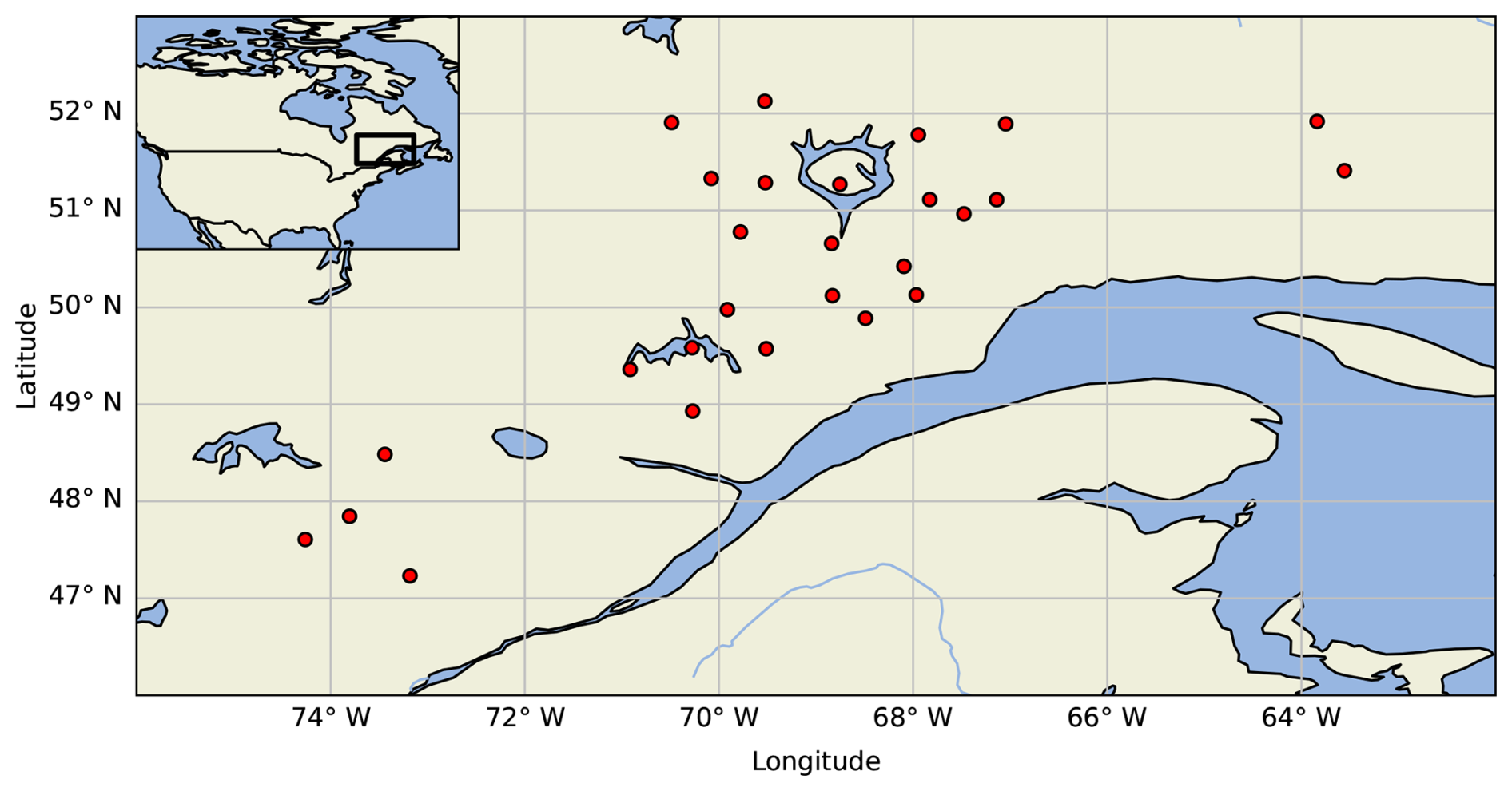
Figure 1 Location of the study sites in eastern Canada. The black square in the top-left inset corresponds to the map domain.

2 Data

2.1 Surface hydrometeorological measurements

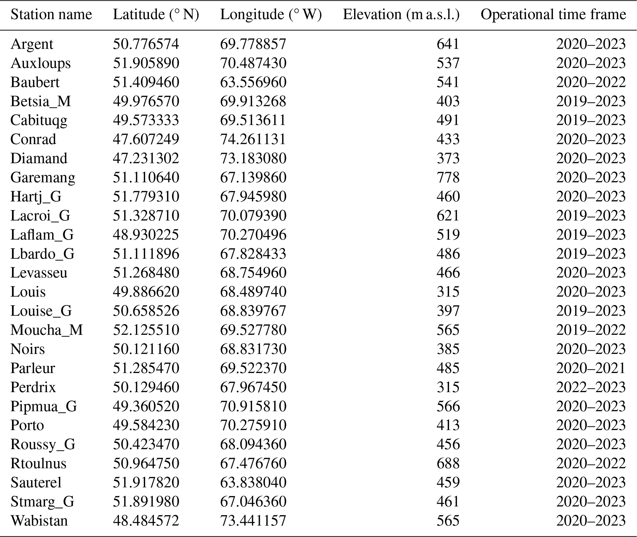
The disdrometer network used for this study was deployed on the north shore of the St. Lawrence River in the province of Quebec, Canada (Fig. 1). It is part of a larger hydrometeorological observation network operated by Hydro-Québec, a public utility responsible for the generation and distribution of electricity in Quebec. The network lies between latitudes of 47.23 and 52.13° N, and longitudes of 63.17 to 75.29° W, spanning an area of roughly 532 594 km². The 27 stations have been in operation for varying periods of time between the years 2019 and 2023, totalling 80 site-years. The site elevations range from 315 to 641 m above sea level (a.s.l.), with an average of 469 m a.s.l. The names, coordinates, and operational time frames for each station are presented in Appendix A.

Figure 2 Distributions of the (a) annual mean temperature, (b) annual mean precipitation, and (c) elevation at the study sites, separated by latitudinal range.

The sites have a mean annual 2 m air temperature of 0.2 °C and a mean annual cumulative precipitation of 902 mm, calculated from 160 site-years of daily observations. Figure 2 illustrates the distribution of annual mean daily 2 m air temperature and precipitation, as well as the elevation of the sites. The annual precipitation decreases with latitude as the northern sites (>51° N) experience an annual mean of 813 mm. The southernmost sites (<49° N) receive more precipitation on average, with an annual mean of 1002 mm. However, the variability observed at these sites is much greater than observed elsewhere. The sites' elevation follows a mostly normal distribution within a 400 m range of the mean, with elevations generally increasing northward. Following the Köppen climate classification, the sites are nearly evenly split between humid continental (Dfb) and humid subarctic (Dfc) climates. The study period spans from 1 October to 1 June of the following year as the chances of snowfall are practically non-existent outside of these dates for the domain of interest.

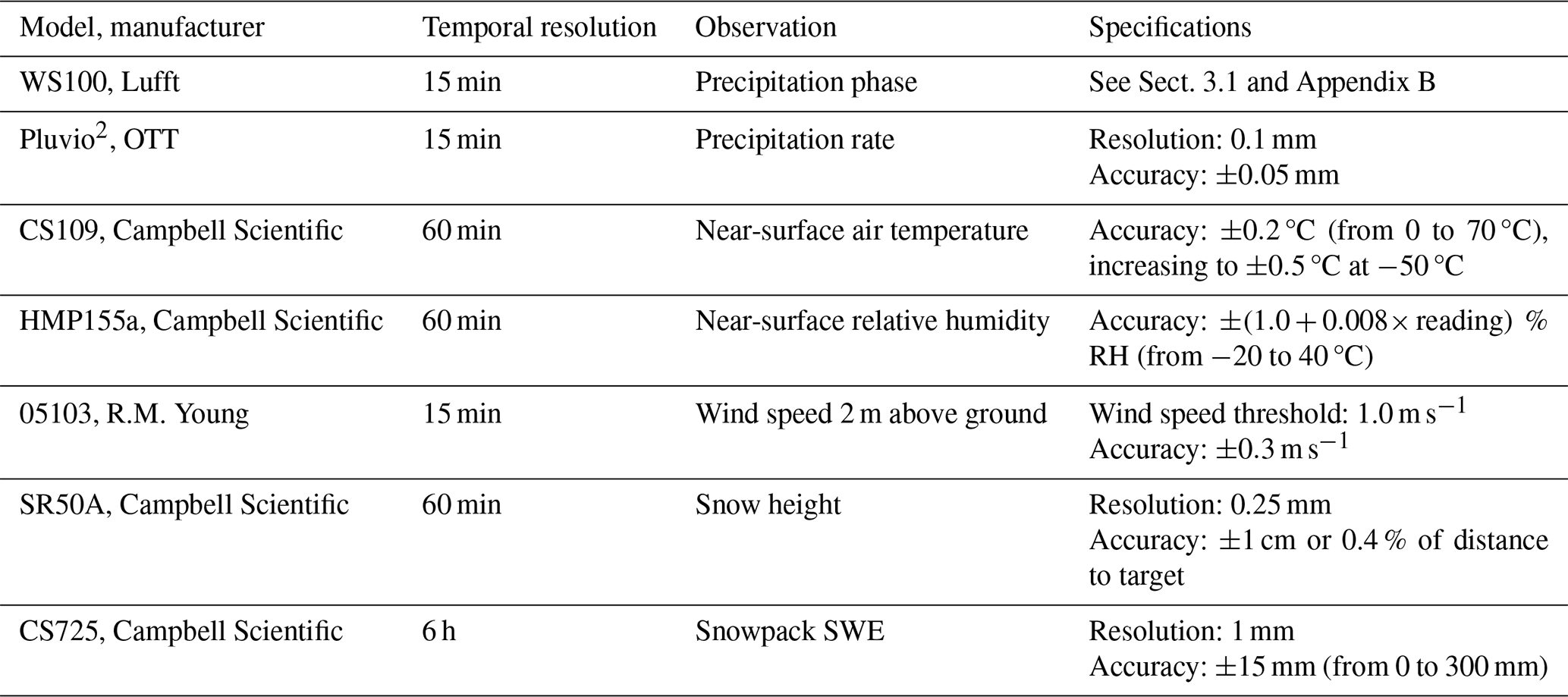
Each site is equipped with a radar-based disdrometer (model WS100, Lufft), providing 15 min phase identification. The WS100 is a K-band (24 GHz) Doppler radar that classifies droplets into 11 size classes between 0.3 and 5.0 mm. The disdrometer assigns World Meteorological Organization (WMO, 2018; Table 4677) weather codes for no precipitation (code 0), rain (code 60), freezing rain (code 67), a mix of rain or drizzle and snow (code 69), and snowfall (code 70). The precipitation phase is identified according to the hydrometeor diameter–fall velocity relationships for water droplets outlined in Gunn and Kinzer (1949), as well as in Locatelli and Hobbs (1974) for solid-phase precipitation particles. Rain and snow fall velocity as a function of measured reflectivity from K-band Doppler radar was investigated in Atlas et al. (1973) and remains an area of active research (e.g. Garcia-Benadi et al., 2020; Kneifel et al., 2011; Löffler-Mang et al., 1999; Sarkar et al., 2015). For simplicity, the phase identifications derived from the diameter–fall velocity relationships are referred as observations in this study. In addition, each site also provides measurements of SWE using a passive gamma ray monitoring system (model CS725, Campbell Scientific) and of snow height using an ultrasonic sensor (model SR50A, Campbell Scientific).

The meteorological observations in this study come from weather stations operated by Hydro-Québec and SOPFEU, the province's wildfire prevention organization. The weather stations provide 15 min accumulated precipitation (model Pluvio² by OTT, equipped with a single-Alter shield), allowing the coupling of precipitation with concurrent disdrometer phase identification. The weather stations measure hourly air temperature (model CS109, Campbell Scientific) and relative humidity (model HMP155a, Campbell Scientific), with sensors mounted 2 m above the ground. Additionally, wind speed and direction are monitored at a 15 min interval with a ground propeller anemometer (model 05103, Young) mounted 2 and 10 m above the ground.

Most of the study sites and weather stations are located in close proximity to each other. Specifically, 67 % of the study sites are within 3 km of or are collocated with the nearest weather station. The remaining stations are between a median distance of 7 km and a maximum distance of 12 km. The only exception is the Auxloups station and the nearest weather station, which are separated by 28 km. To account for the elevation differences between the study sites and weather stations, the air temperature measurements were adjusted using international standard atmosphere methods. The Discussion section will address the uncertainty related to the distance between the study site and the weather station. The temporal resolution and detailed specifications about the study sites' instruments are provided in Table 1.

Table 1 Study site instrument details.

2.2 Reanalysis products

Hourly atmospheric data from the ECMWF Reanalysis v5 (ERA5) (Hersbach et al., 2023) are added to this study's dataset to account for the energy transfer to falling hydrometeors in the atmospheric levels closest to the surface. Furthermore, this will help in assessing the potential performance gain of incorporating gridded data despite the spatial scale discrepancy with local observational data. The added data include temperature profiles for pressure levels of 1000 and 850 hPa. The corresponding geopotential height of these levels is also added to the dataset. The values from the nearest 0.25° × 0.25° grid cell, roughly 28 km × 18 km at the study sites' latitudes, are assigned to every study site. Additionally, the hourly surface atmospheric pressure from ERA5-Land (Muñoz Sabater, 2019) is added to the dataset as it was not measured at the weather stations used in this study. The atmospheric pressure from the nearest 9 km × 9 km grid space is assigned to every study site. From these data, the thickness Δz between the 1000 and 850 hPa layers (m) is calculated with

$$\begin{array}{}\text{(1)}& \mathrm{\Delta }z={\displaystyle \frac{z_{\mathrm{850}}-z_{\mathrm{1000}}}{g}},\end{array}$$

where z₈₅₀ and z₁₀₀₀ correspond to the geopotential heights (m² s⁻²) at the top and bottom of the layer, and g is the gravitational acceleration (9.81 m s⁻²). The layer thickness between the two pressure levels is correlated with the mean temperature of the layer and is also a commonly used variable in operational meteorological models (Feiccabrino et al., 2015). The pressure levels were selected based on their successful use in the classification of the precipitation phase at the surface in prior studies (e.g. Bourgouin, 2000; Shin et al., 2022). The temperature lapse rate Γ (°C km⁻¹) is also calculated:

$$\begin{array}{}\text{(2)}& \mathrm{\Gamma }=-{\displaystyle \frac{\mathrm{\Delta }T}{\mathrm{\Delta }z}}\times \mathrm{1000},\end{array}$$

where ΔT corresponds to the temperature difference between the 850 and 100 hPa layers (°C).

3 Methodology

3.1 Precipitation data processing

The observed 15 min precipitation amounts were compiled at an hourly time step. Each 15 min precipitation data segment was coupled with a disdrometer phase identification. Both valid, non-zero values were required for the data segment to be included in the analysis. A first filter was applied, where hourly precipitation rates <0.2 mm h⁻¹ were considered to be erroneous trace amounts, following standard WMO methodology (WMO, 2018). A second filter was also applied where precipitation rates >110 mm h⁻¹ were considered to be erroneous (Smith et al., 2022). A neutral aggregating filter (Ross et al., 2020) was then applied to eliminate noise and diurnal oscillations in the precipitation data. Additionally, hourly precipitation exceeding 30 mm h⁻¹ was visually inspected. Any data not consistent with nearby stations were considered to be invalid.

The disdrometers used in this study can identify freezing rain and a mix of rain and snow in addition to snow and rain. However, as most hydrological models only interpret the effect of snow and rain, this study focuses on the prediction of solid and liquid precipitation. Therefore, the disdrometer identifications of freezing rain and of a mix of rain or drizzle and snow were aggregated with, respectively, snow and rain events. For example, if hourly precipitation has a fraction of rain and a mix of rain or drizzle and snow, it would be considered to be completely liquid after the aggregation. The selected phase aggregation aims to group the phases that are most similar in terms of hydrological influence and average occurring temperature. These assumptions are supported by an analysis of the effect of each precipitation phase on the snowpack properties (height and snow water equivalent), as detailed in Appendix B.

When solid precipitation was identified, the universal transfer functions of Kochendorfer et al. (2017) were applied to adjust for wind-induced gauge undercatch. To do so, local hourly wind speed and temperature measurements at gauge height were used, which were shown to provide appropriate corrections for sites in boreal climates (Pierre et al., 2019). The solid and liquid 15 min precipitation were then compiled at hourly time steps and were partitioned into liquid- and solid-precipitation fractions, totalling 31 905 data points. The resulting phase partitioning was used to classify the phase of each precipitation event as solid, liquid, or mixed, with respective dataset proportions of 71 %, 22 %, and 7 %.

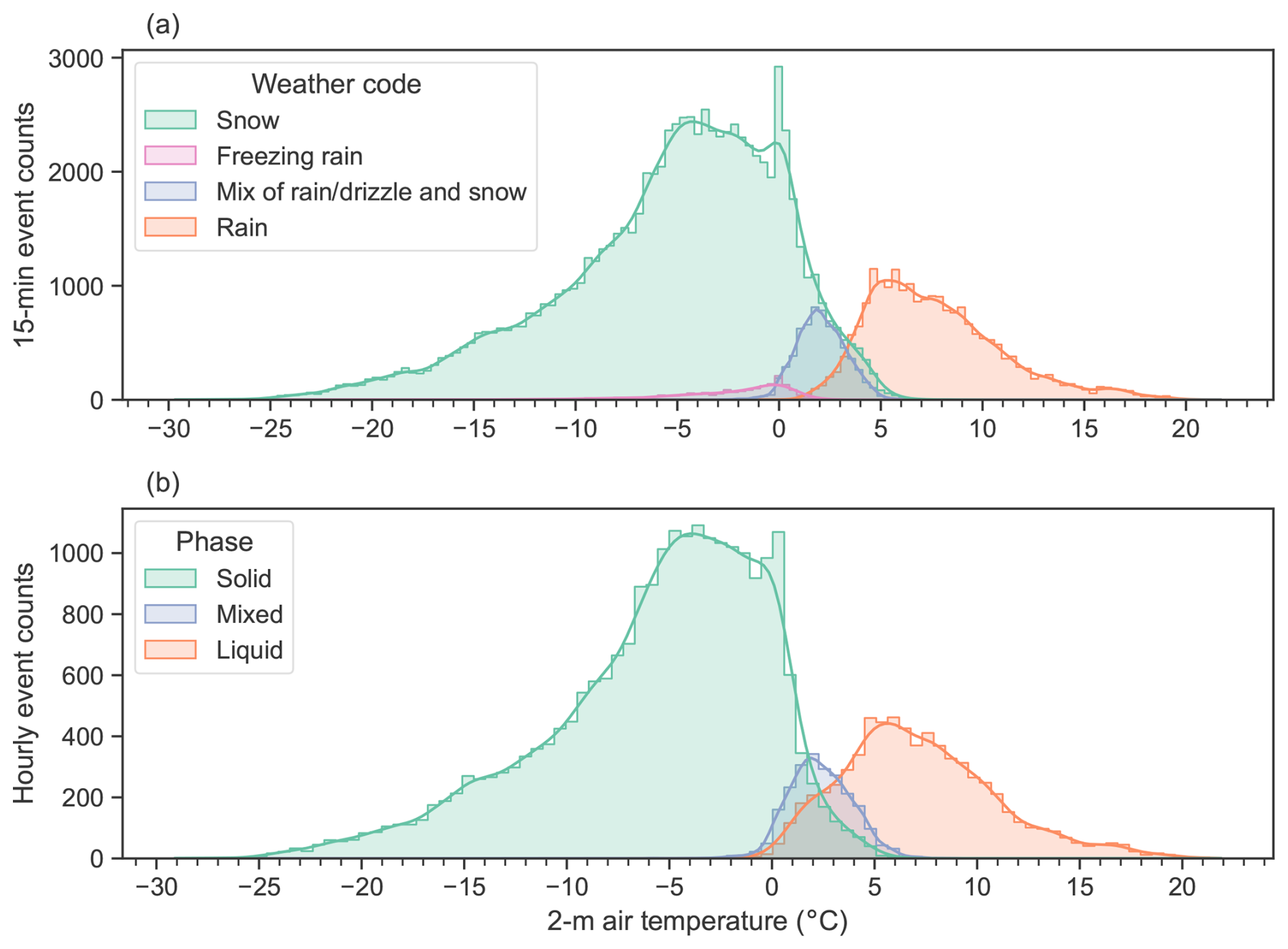
Figure 3 Event counts of (a) the 15 min precipitation phase identified by the disdrometers and (b) the aggregated hourly precipitation phases according to the 2 m air temperature.

Figure 3a shows the phase occurrence of the coupled 15 min precipitation data along an interpolated 15 min 2 m air temperature. The phase occurrence in Fig. 3b shows that it is mostly the mixed and liquid precipitation that are affected by the aggregation and that very few freezing rain events aggregated with snow events result in the snow and solid-phase distributions being very similar. The aggregation of the mix of rain or drizzle and snow with rain results in an increase in liquid precipitation in the 0–5 °C range. Mixed-phase precipitation occurs in the same air temperature range as that of the mix of rain or drizzle and snow, suggesting that this phase is often present in mixed-phase precipitation, thus validating the aggregation. A cursory analysis of the mixed-phase precipitation events revealed that events with a phase transition between snow and a mix of rain or drizzle and snow account for roughly 75 % of the mixed-phase events. Transitions from rain to snow are infrequent and represent roughly 15 % of the mixed-phase precipitation events, while the remainder includes other phase combinations.

3.2 Model performance evaluation

The models presented in this study are evaluated for their ability to correctly predict the precipitation phase using a variety of performance metrics. First, the metrics used to quantify the predictive ability of the models are the precision (PRE) and the recall (REC), as well as the F1 score (Rokach et al., 2023). The combination of precision and recall is commonly used to evaluate model classification performance as the metrics indicate different information. The precision indicates the proportion of correct predictions for a given phase, while the recall indicates the probability of detection for a given phase. By definition, model precision and recall are inversely proportional. The assessment of both metrics informs whether a model overpredicts or underpredicts a given class. For instance, low precision and high recall indicate a class overprediction, while high precision and low recall indicate a class underprediction. Therefore, a model that achieves good performance in both metrics is desirable.

$$\begin{array}{}\text{(3)}& {\displaystyle }\text{PRE}={\displaystyle \frac{\text{TP}}{\text{TP}+\text{FP}}}\text{(4)}& {\displaystyle }\text{REC}={\displaystyle \frac{\text{TP}}{\text{TP}+\text{FN}}}\end{array}$$

In the above, TP, FN, and FP are the true-positive, false-negative, and false-positive counts, respectively, for a given phase. The F1 score, being the harmonic mean of the precision and recall, is a useful metric to quantify the general performance of the model.

$$\begin{array}{}\text{(5)}& \text{F1}=\mathrm{2}\left({\displaystyle \frac{\text{PRE}\times \text{REC}}{\text{PRE}+\text{REC}}}\right)\end{array}$$

These metrics are computed for each precipitation phase separately. A general score is also computed by weighing each phase's score according to its proportion in the dataset. As such, the weighted F1 score is used as a general classification performance metric as it combines both precision and recall and harshly penalizes a poor score in either of them while also considering the dataset imbalance.

Second, the model partitioning performance is evaluated based on the predicted solid- and liquid-precipitation amounts. The metrics used are the coefficient of determination R² and the RMSE. Due to the slightly asymmetric phase distribution and overlap between the phases shown in Fig. 3, different R² values are calculated for the solid- and liquid-precipitation. Thereby, the metrics are calculated on the phase-separated precipitation rather than on the precipitation fraction as the precipitation phase could be solid, liquid, or mixed for a given temperature. Because of the partitioning between solid or liquid precipitation, the RMSE is equal to the root mean squared of the misclassified precipitation. Therefore, the RMSE is the same for both solid and liquid precipitation, and a single score is presented. Finally, the partitioning performance metrics are performed on different subsets of the dataset using a K-fold method. The K-fold validation method is commonly used to assess the variability of model performance with machine learning methods. By using different subsets of the dataset to train and validate the model K times, a more general performance can be assessed. Because of the fewer liquid- and mixed-precipitation events compared to solid-precipitation events, the K fold is also stratified to maintain phase proportions between training and validation sets from fold to fold. As such, in the case of the partitioning validation, the variability of the precipitation amounts from fold to fold must be considered. The performance metrics are repeated until the variance of the partitioning performance metrics stabilizes. In this case, the validation was performed with 5-fold validation and was repeated six times for a total of 30 validation folds.

3.3 Phase-guided probabilistic precipitation phase model

Machine learning algorithms are powerful tools for building classification and regression models. Random forests (Breiman, 2001) are commonly utilized in the environmental sciences due to their simple implementation and lower susceptibility to overfitting compared to other models. The model is based on decision trees, where variables are randomly chosen at each node to create a prediction. Therefore, the decision trees, each unique due to randomness, provide predictions that are ultimately aggregated to generate a final well-informed prediction.

Figure 4 Development and validation methodology for the phase-guided-partitioning model.

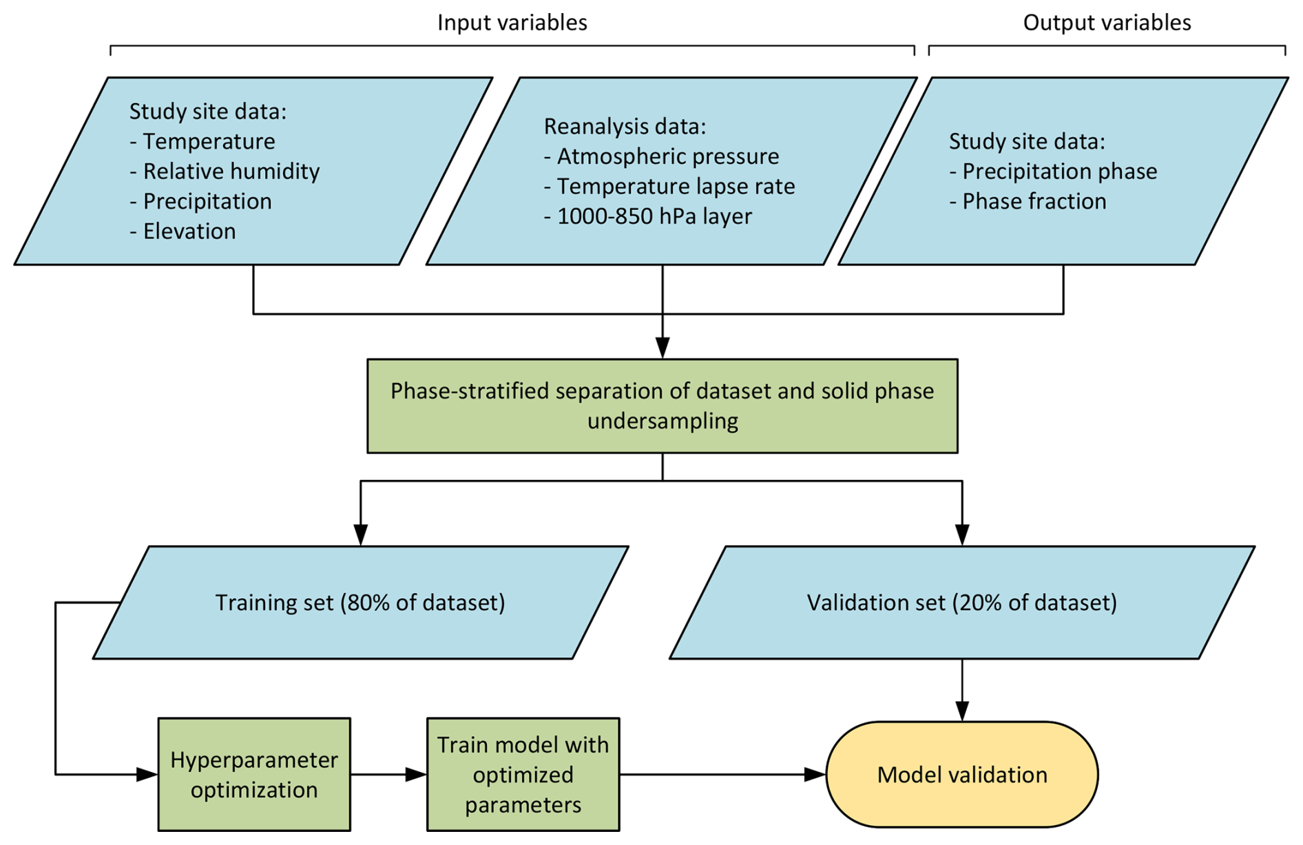
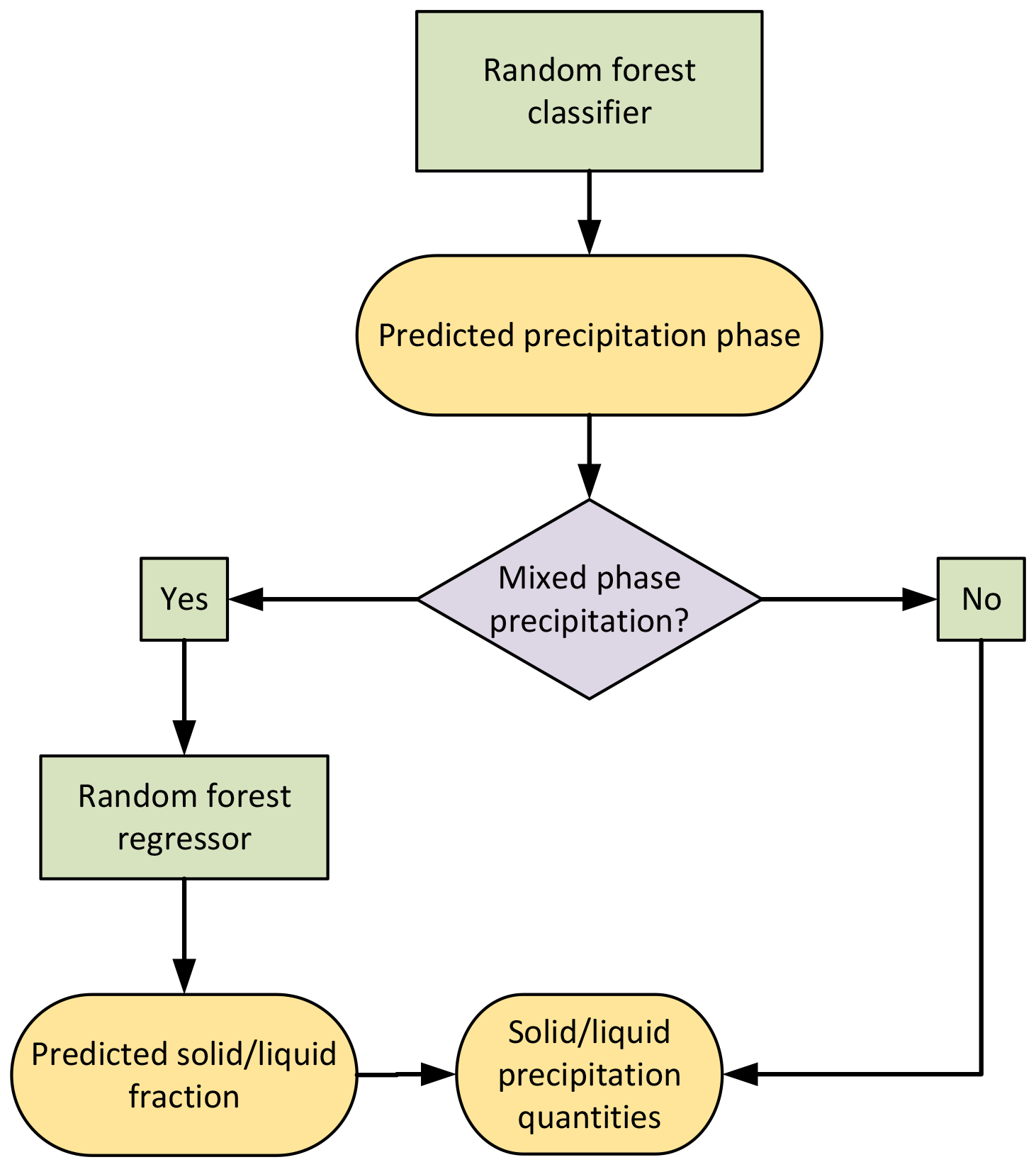
Given the overlapping phases of the dataset, a random forest (RF) classifier is used to predict the precipitation phase with a probabilistic approach. The procedure to develop the RF model is illustrated in Fig. 4. To address the phase type imbalance, the data were adjusted by undersampling the solid phase and increasing the weight of both liquid- and mixed-precipitation phases in the dataset. To achieve this, only data points with air temperatures between −4 and 8 °C were kept in the analysis. The phase proportions resulting from the undersampling are 60 % solid, 26 % liquid, and 14 % mixed. The data were then split using an $\mathrm{80}/\mathrm{20}$ ratio between the training and validation sets, respectively, resulting in 13 339 data points for training and 3335 for validation. To account for the prevalence of solid-precipitation samples, the training and validation sets were stratified to maintain the aforementioned phase proportions between the two subsets (60 % solid, 26 % liquid, 14 % mixed). Hyperparameters were optimized on the training set to increase the model performance and to reduce the chance of overfitting by using a stratified 5-fold cross-validation and maximizing for a weighted F1 score. The RF classifier was then retrained on the entire training dataset and was ready for use on the validation set.

While the precipitation partitioning is straightforward when the predicted phase is either solid or liquid, it is less so for a predicted mixed phase, where a solid- and liquid-precipitation fraction must be assigned. Thus, in the case of a predicted mixed phase, an RF regression model is developed following the same steps described above. The loss function used to optimize the regression model parameters is the mean-squared error (MSE) to increase the penalty on larger errors. The phase-guided-partitioning model predicts a precipitation phase, as well as a solid- and liquid-precipitation partitioning according to the predicted phase, with the complete process illustrated in Fig. 5.

Table 2 Listing of the input variables used in the tested PGP models.

Figure 5 Phase-guided-partitioning model structure.

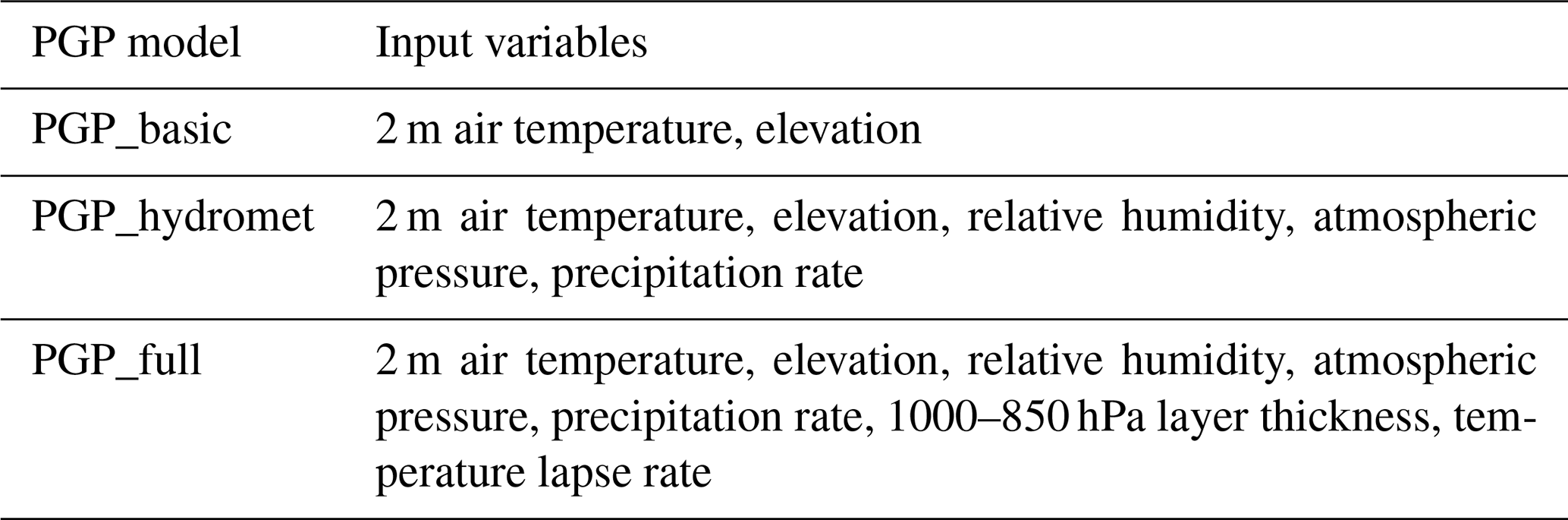
Multiple PGP models using a combination of atmospheric variables were developed. The subsets of input variables of the PGP models accommodate different levels of data availability, ranging from the strictest minimum data requirements (e.g. in an operational context) to atmospheric variables, with each subset fully incorporating the previous subsets (see Table 2). This approach will help to quantify the impact of some atmospheric variables that are not measured at surface weather stations. The simplest model, PGP_basic, includes only 2 m air temperature and site elevation. Next, PGP_hydromet includes all related near-surface hydrometeorological data, such as relative humidity, atmospheric pressure, and precipitation rate. Finally, the PGP_full model, as discussed in the previous sections, incorporates atmospheric data from reanalysis, specifically the thickness of the 1000–850 hPa layer and the temperature lapse rate.

3.4 Benchmark phase-partitioning models

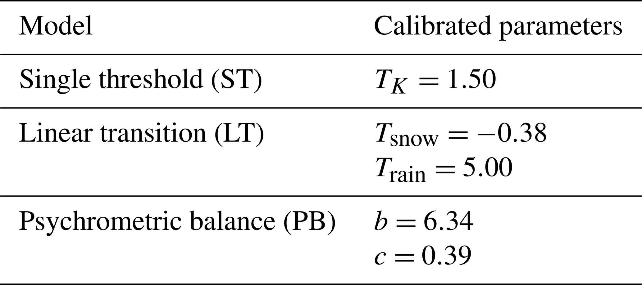
The benchmark models used for this study are common methods of increasing complexity found in hydrological models. First, a single 2 m air temperature threshold (ST) model is used as a baseline comparison. This model separates precipitation into solid and liquid phases based on a calibrated air temperature threshold. While this type of model is widely used, it is generally associated with larger partitioning errors on a seasonal basis (Harpold et al., 2017). Second, a linear-transition (LT) model is used. It allows for mixed-phase precipitation while still being of low complexity. LT partitions the solid and liquid precipitation according to a linear relationship between a snow and rain temperature threshold. Finally, the psychrometric-energy-balance (PB) model is used, which is a phase-partitioning method based on the mass energy and energy balance of a sublimating ice sphere that integrates the relative humidity to estimate the hydrometeor temperature (Harder and Pomeroy, 2013). The estimated hydrometeor temperature is then used as an input in a two-parameter curvilinear relationship. All three benchmark models are calibrated individually with the least squares method, minimizing the error with the observed solid-phase fractions. The models and their calibrated values are given in Appendix C. The precipitation phase can then be inferred from the predicted fractions. In other words, a mixed phase will be predicted in the instance of non-zero solid and liquid fractions, otherwise the predicted phase is either solid or liquid. Previous studies that employed probabilistic models based on direct phase observations (e.g. Behrangi et al., 2018; Jennings et al., 2018) were not included as benchmark models. Mixed-phase precipitation is typically excluded from such studies as there is no effective method to accurately partition the precipitation due to the categorical nature of direct phase observations. The above considerations make such models difficult to compare with the PGP models presented in this study.

3.5 Input variable importance analysis

A common way to interpret input variable importance for a machine learning model is to use permutation importance, which helps in decreasing the black-box aspect of machine learning algorithms (McGovern et al., 2019). The performance of the model is computed according to a chosen scoring scheme. Each variable of the model is then shuffled individually. The goal of this step is to break the relationship between a variable and the desired prediction. After each shuffle, a performance score is calculated to show the decrease in model performance. This process is then repeated several times to account for data variability. Thus, the relative importance of each input variable to the model can be quantified with the resulting performance decrease. Permutation importance analysis provides only the importance of an input variable to the model and not the inherent information provided by that variable. However, when shuffling a variable that is highly correlated to another, the model can still find the shuffled variable's information when performing permutation importance analysis. In practice, this is an important consideration as it means the importance of either or both input variables can be lower. This analysis offers insight into the crucial variables for the PGP models and how they can be further improved.

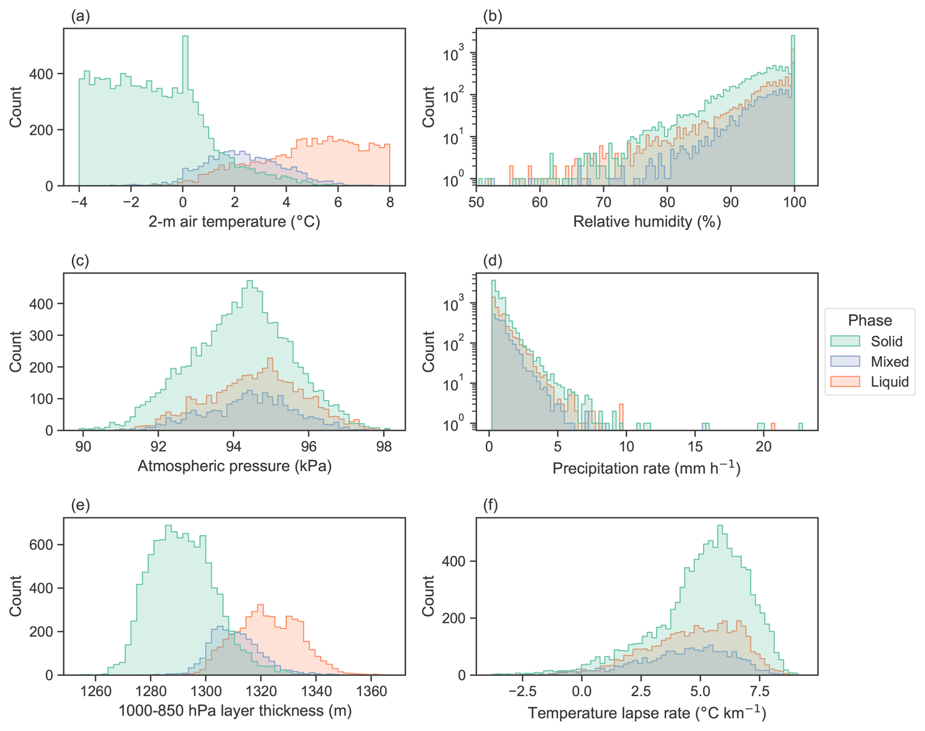
Figure 6 Input distributions separated by phase of (a) 2 m air temperature, (b) relative humidity, (c) atmospheric pressure, (d) precipitation rate, (e) 1000–850 hPa layer thickness, and (f) air temperature lapse rate.

4 Results

4.1 Dataset analysis

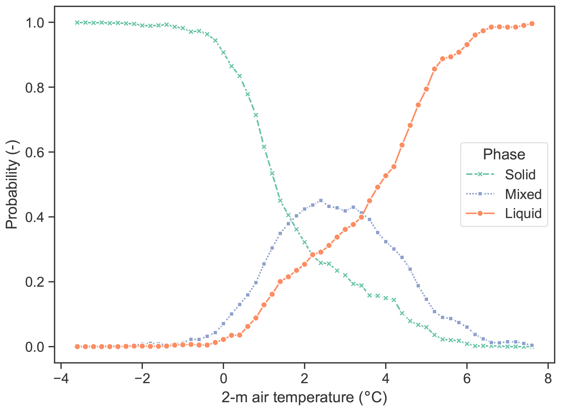
The distribution of the hydrometeorological variables categorized by precipitation phase is displayed in Fig. 6. The temperature distributions show a significant overlap between all three phases from 1.5 to 3.6 °C, similarly to that reported in Jennings et al. (2023). Mixed-precipitation probability peaks at approximately 2.4 °C. The distribution of relative humidity reveals that precipitation is associated with near-saturation water vapour conditions, with a median value of 97 %, regardless of the precipitation phase. The mean precipitation rate is generally low at 0.9 mm h⁻¹. The median precipitation rate for mixed-phase events is generally the highest at 0.8 mm h⁻¹, followed by that of liquid-phase events at 0.7 mm h⁻¹ and that of solid-phase events at 0.6 mm h⁻¹. Atmospheric pressure distributions are similar for both liquid- and mixed-phase precipitation events. The mean air pressure during the solid-precipitation events is comparable to that of the other phases, but there are more events between 90 and 92 kPa. The distribution for the thickness of the 1000–850 hPa layer closely mirrors that of air temperature, given their general correlation. The temperature lapse rate averages 4.9 °C km⁻¹, and distributions, especially of solid precipitation, show a bias toward the standard atmospheric lapse rate of 6.5 °C km⁻¹.

The overlap of the phase distributions for each input variable, most notably the air temperature, indicates that a probabilistic approach is appropriate for predicting the precipitation phase. Indeed, between approximately 0 and 4 °C, solid and liquid precipitation may occur separately or coexist. According to findings in previous studies, precipitation over land is more likely to occur in a single phase than in mixed-phase precipitation (Dai, 2008; Froidurot et al., 2014), as is the case in this study, where only 13 % of the precipitation data points are mixed phase. There is, however, a narrow 2 m air temperature range, between 2 and 2.5 °C, where mixed-phase probability exceeds the probability of single-phase precipitation. An appropriate phase-partitioning model must thus accurately predict the phase in the temperature interval where solid-, liquid-, and mixed-precipitation occurrences overlap while also providing accurate partitioning when needed.

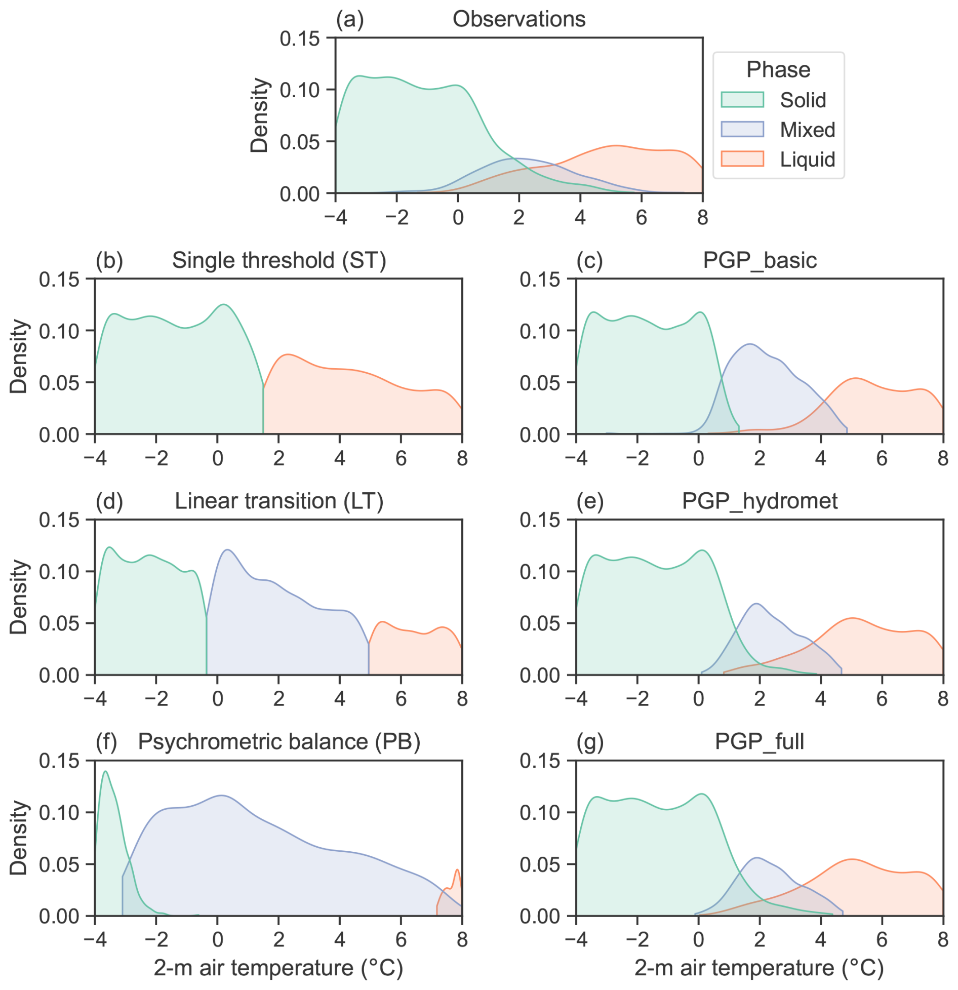
Figure 7 Hourly phase distributions according to 2 m temperature of the (a) observations, (b) single threshold, (c) PGP_basic, (d) linear transition, (e) PGP_hydromet, (f) psychrometric balance, and (g) PGP_full. PGP model details are summarized in Table 2.

Table 3 Weighted classification scores for single-threshold (ST), linear-transition (LT), psychrometric-balance (PB), and phase-guided-partitioning PGP models. PGP model details are summarized in Table 2.

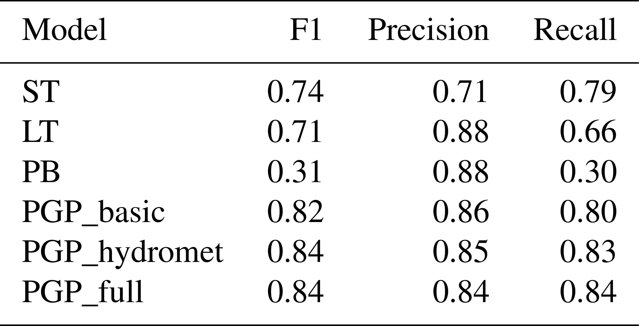
4.2 Phase classification

Figure 7 shows the phase density distribution of the benchmark models and the PGP models in comparison to the observations. The corresponding classification scores of the models, which were weighted to reflect the precipitation phase proportions in the dataset, are presented in Table 3. The phase density distributions show the limitations of benchmark phase-partitioning models, namely that the mixed phase is absent or overrepresented compared to the observations. However, ST performs well in all three metrics due to the low likelihood of mixed-phase occurrence. When evaluating the overall classification performance using the F1 score, LT follows ST because of a disparity between precision and recall that affects its F1 score. The lower recall score for LT can be attributed to its overprediction of the less frequent mixed phase, which, in turn, negatively affects the recall of other phases. This enhances the model's weighted precision by decreasing the number of false positives in non-mixed-phase prediction. The same reasoning can be more extensively applied to PB's weighted scores. The mixed phase's overlap with other phases significantly decreases the model's overall recall. Due to the relationships used to create the benchmark models, the overlap between all three phases is not accurately represented. By including relative humidity, PB can model phase overlap, but this does not improve the modelled phase distribution density with respect to the observations.

The weighted F1 score for the PGP models shows that they have a more robust general performance as they have high weighted precision and recall scores while having a small disparity between both scores. The PGP models reproduce the observed phase overlap well but overpredict the mixed phase slightly, affecting both the solid- and liquid-phase predictions. PGP_basic exhibits the greatest mixed-phase overprediction, while the difference between PGP_hydromet and PGP_full is marginal. This result suggests possible improvements to PGP models, particularly for mixed-phase precipitation.

Figure 8 Model phase classification metrics separated by (a) the solid, (b) the mixed, and (c) the liquid phase. PGP model details are summarized in Table 2.

The phase-separated classification metrics provide further insight into the performance of the models, as shown in Fig. 8. The F1 score provides an overall performance for each phase prediction. PGP_full has the best F1 scores for both the solid and liquid phases, while PGP_hydromet has a higher F1 for the mixed phase. PGP_basic is generally the third best-performing model in terms of F1 score, except for the solid phase, where ST outperforms it. While it is not able to predict the mixed phase, ST has the highest scores for the liquid- and solid-precipitation phases out of the benchmark models. This is probably because mixed-phase precipitation events constitute only roughly 13 % of the samples; this low proportion does not significantly decrease the model's performance. LT performs slightly worse than ST for both solid- and liquid-phase F1 scores but has the highest mixed-phase F1 score out of the benchmark models.

PB's poor F1 scores are explained by the overlaps between the phases shown in Fig. 7. The model allows the predicted mixed phase to overlap with the predicted solid and liquid phases, which is the opposite behaviour compared to the observed phase density, where mixed-phase precipitation mostly exists in the solid- and liquid-phase overlap. Given the modelled phase density and the resulting classification scores, the phase prediction abilities of both LT and PB suffer from overprediction of the mixed phase. This is evidenced by the significant disparity between the precision and recall scores of LT and PB for the mixed phase. A high recall score signifies that the model minimizes the number of false negatives, which negatively affects the model's precision. Thus, overpredicting the mixed phase greatly reduces the models' precision for the mixed phase while greatly increasing their recall for the mixed phase. Conversely, the conservative prediction of the liquid and solid phases increases the precision of the model but decreases the recall for both phases.

Although they are not always the best models in terms of either precision or recall, the PGP models have the best general performance, making them more reliable for phase prediction. Thus, PGP models significantly reduce phase identification error by showing high precision and recall, with small disparities for solid- and liquid-phase prediction. However, PGP's main distinguishing feature is its general ability to predict mixed-phase precipitation. Furthermore, the disparity between the precision and recall scores for the mixed phase is much smaller than for the other models studied, indicating that the overprediction of the mixed phase is much less severe for PGP.

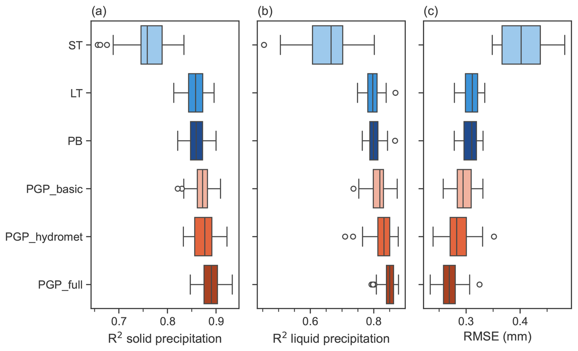
Figure 9 Model regression performance in (a) R² for solid precipitation, (b) R² for liquid precipitation, and (c) RMSE. PGP model details are summarized in Table 2.

4.3 Precipitation partitioning

Figure 9 displays how the regression metrics vary across validation folds. The precipitation rate variability has a significant impact on ST's performance, making its ability to partition precipitation highly variable from winter to winter. In contrast, LT and PB exhibit better performance than ST due to their ability to partition the solid and liquid phases, with much less variability in performance. The variability of R² for liquid precipitation is lower for LT and PB than for solid precipitation because fewer of these events occur. For all regression metrics, LT and PB have similar performances. This is most likely due to the very humid environment, which decreases the difference between the 2 m air temperature and the hydrometeor temperature computed for PB.

Table 4 Average regression scores for single-threshold (ST), linear-transition (LT), psychrometric-balance (PB), and phase-guided-partitioning (PGP) models. PGP model details are summarized in Table 2.

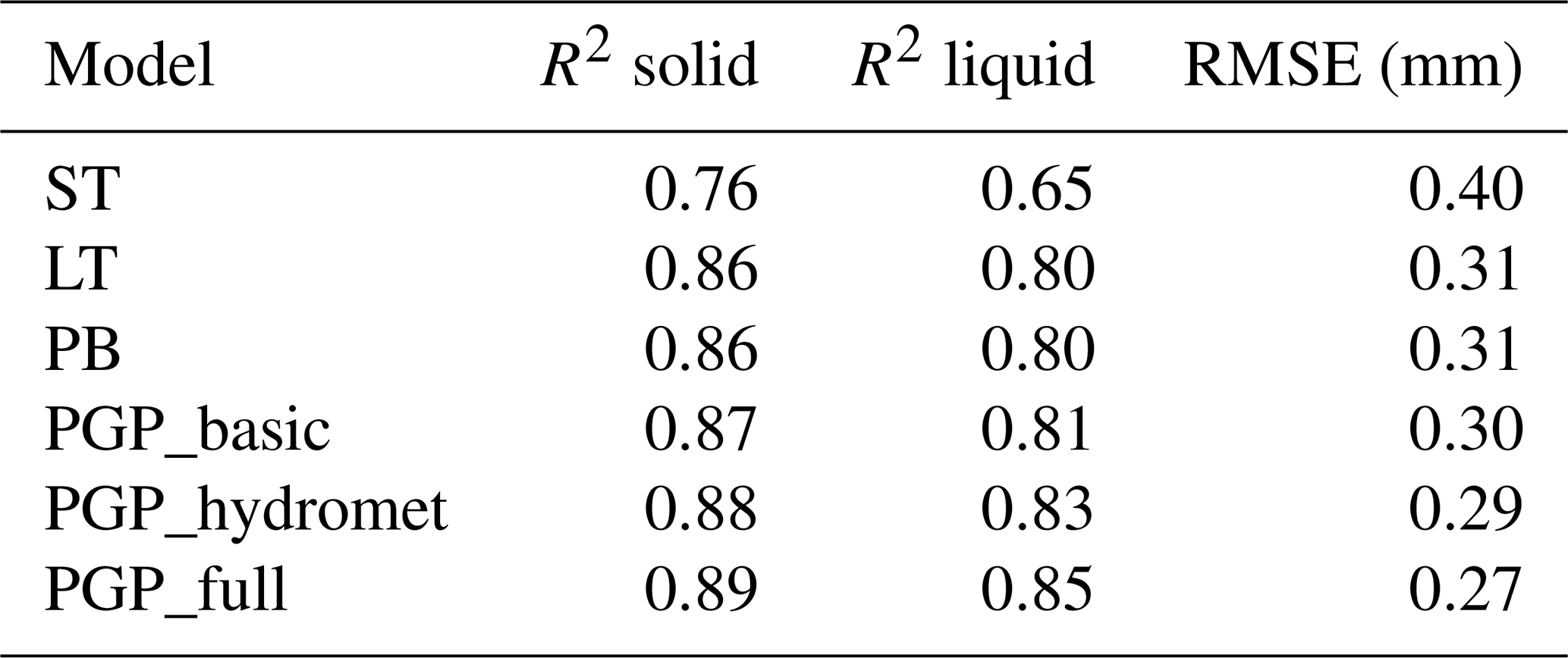
The average regression metrics in Table 4 show the partitioning performance of the various models. All models have a high R² for solid precipitation, likely due to the abundance of solid precipitation. However, model performance decreases for liquid precipitation R², with ST being significantly lower than for other models. This trend is also observed for the RMSE. While ST is the worst-performing model, LT, PB, and PGP_basic perform similarly in all regression metrics. The inclusion of hydrometeorological data in PGP_hydromet leads to a slight increase in performance. Lastly, the inclusion of atmospheric data in PGP_full improves performance compared to the other models.

Generally, the performance of PGP_basic is similar to that of LT and PB, with slight differences. PGP_basic is more variable in its performance for solid-precipitation R² and RMSE. This variability can be attributed to the misclassification of precipitation events due to its limited input variables. The R² scores for PGP_hydromet are less variable than for PGP_basic, while its RMSE is the most variable out of the PGP models. PGP_full exhibits the lowest variability for both R² and is the only PGP model with RMSE variability similar to the benchmark models LT and PB.

The broader RMSE score range of the PGP models highlights the impact of misidentified phases. Misidentification can be more costly than for a benchmark model that systematically separates precipitation into solid and liquid phases for temperatures where mixed-phase events are possible. Furthermore, models such as LT and PB achieve partial accuracy in phase partitioning by forcing mixed-phase precipitation, but if a PGP model misclassifies the phase, the entire precipitation event may be incorrectly partitioned. However, PGP models do show that phase identification prior to phase partitioning can reduce the overall error of a model for both solid and liquid precipitation. This suggests that improved phase identification, specifically with mixed-phase prediction, could greatly enhance the accuracy of precipitation partitioning from PGP models.

Figure 10 Correlation matrix of PGP_full input variable pairs.

4.4 Input variable importance

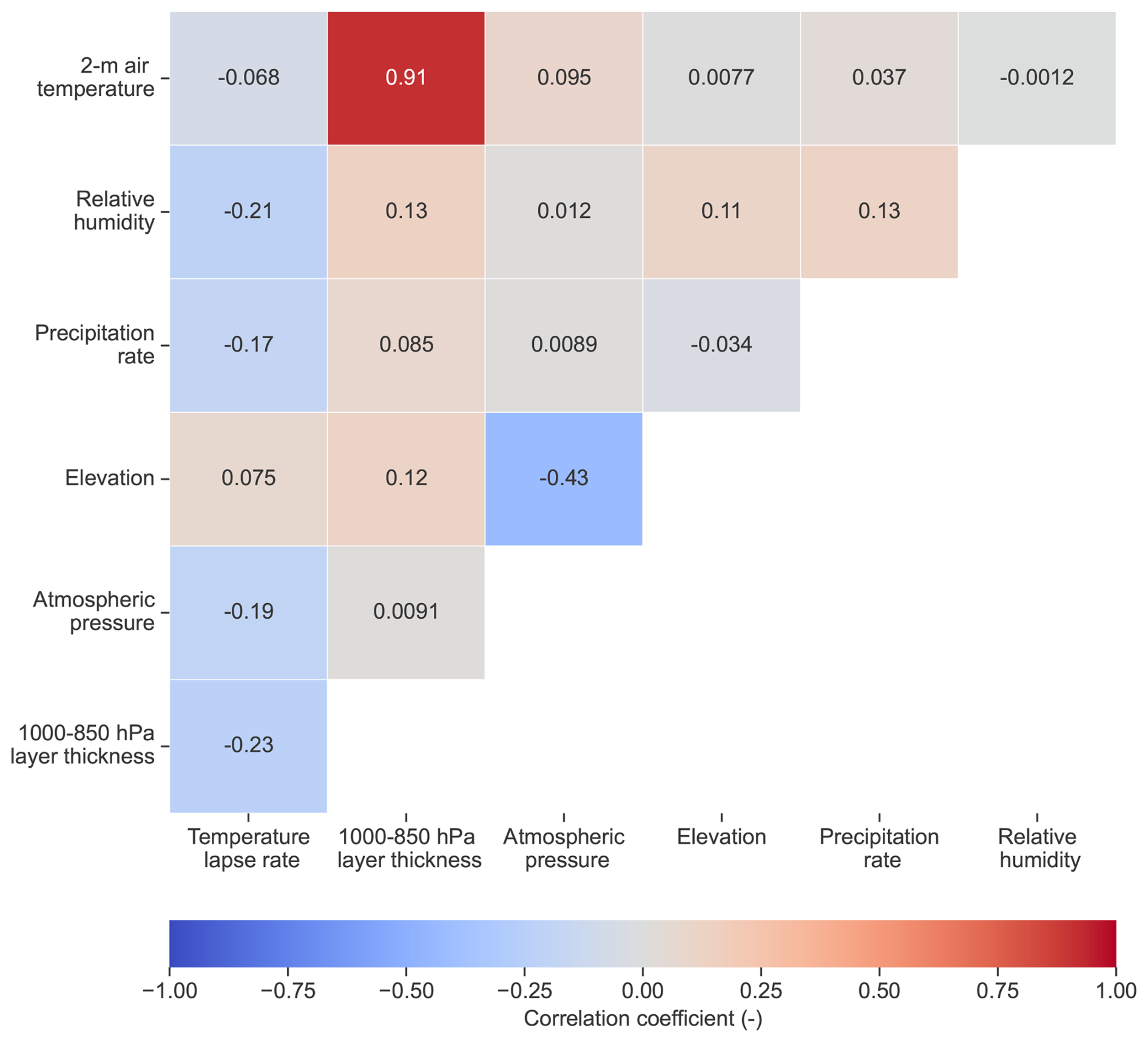
Figure 10 shows the correlation matrix of PGP_full input variables. While the correlation of most input variable combinations is low, the 2 m air temperature and 1000–850 hPa layer thickness are highly correlated. The layer thickness is affected by environmental temperatures as the air density is inversely proportional to its temperature. Therefore, as temperatures increase, the distance between two pressure levels also increases. There is a moderate negative correlation between elevation and air pressure, probably because of the small range of study site elevations. The temperature lapse rate has a small correlation with almost all features.

The scoring scheme for permutation importance must be carefully selected according to the model and use case. In this instance, the PGP models tend to overpredict the mixed phase, which also negatively impacts their ability to predict the other phases. In turn, this also affects the models' partitioning errors, which indicates that their overall performance is reliant on accurate phase classification. For these reasons, the chosen scoring scheme for the permutation importance is the weighted F1 score, used to consider the classification of the imbalanced phase dataset.

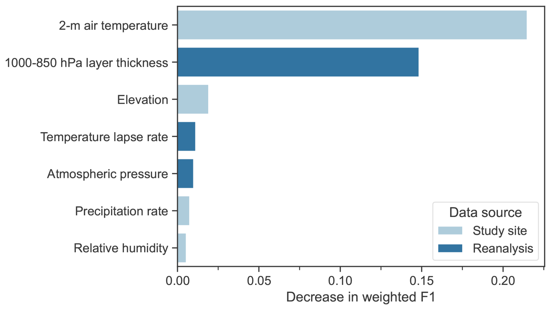
Figure 11 Permutation importance of PGP_full input variable, showing the decrease in the model's weighted F1 score.

Figure 11 shows the permutation importance of PGP_full input variables and the resulting decrease in the weighted F1 score in relation to the validation set. The 2 m air temperature is the most important variable, with its permutation decreasing the score by more than 0.2. The second most important variable is the 1000–850 hPa layer thickness, a result shared by Shin et al. (2022). Because of its high correlation with the 2 m air temperature, it is difficult to interpret the real importance of this variable. In terms of classification performance, the addition of this variable seems to provide small improvements, as shown by the differences in classification metrics between PGP_hydromet and PGP_full.

For the remaining variables, the importance decreases sharply. However, while the individual importance of the variables is low, they improve the phase classification when combined. This suggests that the additional variables used in PGP_full are likely to improve mostly mixed-phase prediction, which is supported by the model's performance in Sect. 4.2. The elevation is used to approximate the atmospheric pressure of a site and can improve phase partitioning (e.g. Ding et al., 2014; Behrangi et al., 2018). Furthermore, atmospheric pressure is often cited as an important variable for phase partitioning (e.g. Behrangi et al., 2018; Dai, 2008; Jennings et al., 2018). The thinner air in low-pressure environments allows snow to reach the ground faster. The temperature lapse rate provides key information regarding the amount of energy the hydrometeors absorb before reaching the ground.

The precipitation rate has a minor impact on the performance of the model. Nevertheless, it may hold significance for the prediction of the mixed phase. The precipitation rate is linked to the precipitation phase as it increases the energy required to completely melt falling precipitation (Froidurot et al., 2014; Thériault et al., 2010). However, its effect is minimal, most likely due to the small proportion of mixed-phase events. Finally, the model ranks relative humidity as the least important feature. This outcome is unexpected because relative humidity was shown to have a significant effect on phase partitioning (e.g. Behrangi et al., 2018; Jennings et al., 2018). One explanation could be the high percentage of data points near water vapour saturation, resulting in the variable being less regionally significant than more heterogeneous regions such as mountain ranges. Besides, this could account for the PB model's underwhelming classification accuracy since it utilizes relative humidity to determine the precipitation phase and due to the fact that it was developed for the drier climate near the Canadian Rockies.

5 Discussion

5.1 Model performance and input variable importance

The classification and regression metrics of the PGP models show that phase classification prior to phase partitioning reduces the partitioning error of solid and liquid precipitation while also providing a more reliable phase prediction than benchmark models. The use of radar-based disdrometer measurements enabled the partitioning step of the model by providing precipitation fractions for mixed-phase events, a flaw mentioned in other studies (Froidurot et al., 2014; Jennings et al., 2018). Out of the benchmark models, ST displayed the best classification performance despite not allowing for mixed-phase precipitation. The tendency of overpredicting the mixed-phase precipitation of both LT and PB reduced their overall classification performance. This general behaviour was also observed in Leroux et al. (2023), where simpler methods outperformed methods based on a precipitation phase fraction. However, ST showed significantly worse partitioning performance compared to LT and PB. The limitations of precipitation-fraction-based models are highlighted by the fact that LT and PB were the worst-performing phase classification benchmark models despite being the best partitioning benchmark models. These models are calibrated to minimize partitioning error, but, in doing so, they are biased toward predicting mixed-phase precipitation. The mixed-phase prediction of the benchmark models could be artificially constrained to reduce overprediction and to improve classification performance. Such constraints would, however, increase the benchmark models' partitioning error, given that they were calibrated according to solid-precipitation fractions. Therefore, there is a trade-off between classification and partitioning error for precipitation-fraction-based models such as LT and PB.

PGP_basic, while showing an improvement in phase classification, did not significantly outperform the partitioning of the benchmark models LT and PB. PGP_hydromet showed improved phase classification, notably for the mixed phase, and partitioning. PGP_full showed a further increase in overall performance while also reducing the partitioning error variability. However, all PGP models tended to overpredict the mixed phase, as shown in Fig. 7. Reducing the overprediction of the mixed phase is a persistent challenge in improving precipitation phase modelling, as noted in previous studies (Casellas et al., 2021; Leroux et al., 2023).

The permutation importance analysis showed that most input variables used, apart from the 2 m air temperature, are of low importance. However, the classification performance improvements in PGP_hydromet and PGP_full show the cumulative importance of the additional variables used, most notably for mixed-phase prediction. Despite many studies demonstrating its impact on precipitation phase, relative humidity was found to be the least important factor. This is likely due to the regional homogeneity, with most observations occurring near liquid water vapour saturation. The site elevation was considered to be important for phase classification, even though it is a constant variable. This suggests that an atmospheric pressure estimated by the elevation could provide enough relevant information to improve phase classification. Still, out of the hydrometeorological variables, the atmospheric pressure had the most impact on phase classification performance. This is in line with other studies that found that it has a significant impact on the precipitation phase (e.g. Behrangi et al., 2018; Dai, 2008; Jennings et al., 2018), although this is generally to a lesser extent than relative humidity when considering the regional variability.

The precipitation rate's low importance is most likely because it affects mixed-phase prediction and thus has little impact on the overall performance. According to Thériault et al. (2010), higher precipitation rates raise the likelihood of larger hydrometeors, which require more energy to melt. Consequently, there is an increased likelihood of mixed-phase precipitation occurring in the form of partially melted hydrometeors. As noted by Feiccabrino et al. (2015), higher precipitation rates can lead to snowfall happening at warmer temperatures due to the presence of unstable air below the isothermal layer.

The permutation importance of the 1000–850 hPa layer thickness is second to the 2 m air temperature. However, because of the high correlation of the pair of variables combined with the moderate classification improvement in PGP_full, the real importance of the 1000–850 hPa layer is most likely to be low. While the importance of the temperature lapse rate is low, the partitioning results demonstrated that incorporating gridded atmospheric variables alongside local observations led to a reduction in the variance of the regression performance. This finding is noteworthy because few studies, as pointed out by Harpold et al. (2017), have explored the impact of incorporating atmospheric reanalysis data into phase modelling. Froidurot et al. (2014) indicated that models using atmospheric data did not greatly improve the phase prediction, as is the case in this study's classification performance. Furthermore, Dai (2008) emphasizes the terrain-dependent nature of lapse rates. Thus, even though the study sites in the region are relatively similar in terms of terrain, the importance of lapse rates in the modelling process was still significant, contrarily to the fairly homogenous relative humidity measurements.

5.2 Coupled precipitation data uncertainty

There are uncertainties regarding the results due to the dataset and assumptions employed. Hydrological models commonly limit the precipitation phases to solid or liquid. Nonetheless, this dataset includes a considerable quantity of mixed snow and rain or drizzle events, and it is uncertain how hydrological models should handle this precipitation phase. The phase aggregation step considered the behaviour of the snowpack following the different phases detected by the disdrometers. Following a mix of rain or drizzle and snow, the SWE and snow height tended to decrease, a snowpack response similar to that following a rain event. It can be inferred that this type of precipitation is likely to be dominated by rainfall given the warm temperature at which it occurs and the ensuing effects on the snowpack. However, it is probable that this interpretation is specific to the disdrometers used in this study unless evidence to the contrary emerges. However, phase identification errors have the potential to introduce uncertainties into the results, notably in the case of mixed-phase precipitation. To measure this uncertainty, it is recommended that studies be conducted using collocated WS-100 disdrometers and other well-documented options such as laser disdrometers to assess the differences between ground-truth-providing instruments (Harpold et al., 2017).

Figure 12 Confusion matrix of the precipitometer and disdrometer 15 min precipitation hit rate, normalized over the precipitometer observations. The upper-left metric is the probability of detection, the upper-right metric is the miss rate, and the lower-left metric is the false-alarm rate.

Another source of uncertainty arises from the coupling of precipitation amounts and phase observations. Fehlmann et al. (2020) demonstrated that laser disdrometers have low missed-event and false-alarm rates for sub-daily integration times compared to precipitometers, but no such study was conducted with the radar-based disdrometers of this study. Additionally, the study by Fehlmann et al. (2020) was carried out in a site sheltered from the wind, implying that the wind-induced gauge undercatch could not be studied. In turn, the wind could influence the missed-event and false-alarm rates of this study's instruments. In this study, data segments where either the precipitation gauge or disdrometer did not detect any precipitation were discarded. Figure 12 displays the hit rate of both the instruments at the initial 15 min intervals and shows that the instruments' hit rates are generally in agreement. The instrument hits were normalized over the precipitation gauge observations to compute relevant agreement metrics. The precipitation gauge is considered to be ground-truth as it would be used in conjunction with a precipitation phase model, and phase observations are rare in an operational context.

Precipitation data segments of 0.1 mm coincide with 38 % of the disdrometer misses. Assuming that a significant portion of this precipitation data would be labelled as trace amounts when resampled at the hourly interval (<0.2 mm), the probability of missed events is likely to be lower in reality. Multiple factors could account for disagreements between the instruments, including the effect of wind, which likely varies from instrument to instrument, and the fact that certain stations are not collocated or nearby. However, studies on the environmental effects on the disdrometer performance are lacking, and this would require more detailed investigation, as outlined in Harpold et al. (2017).

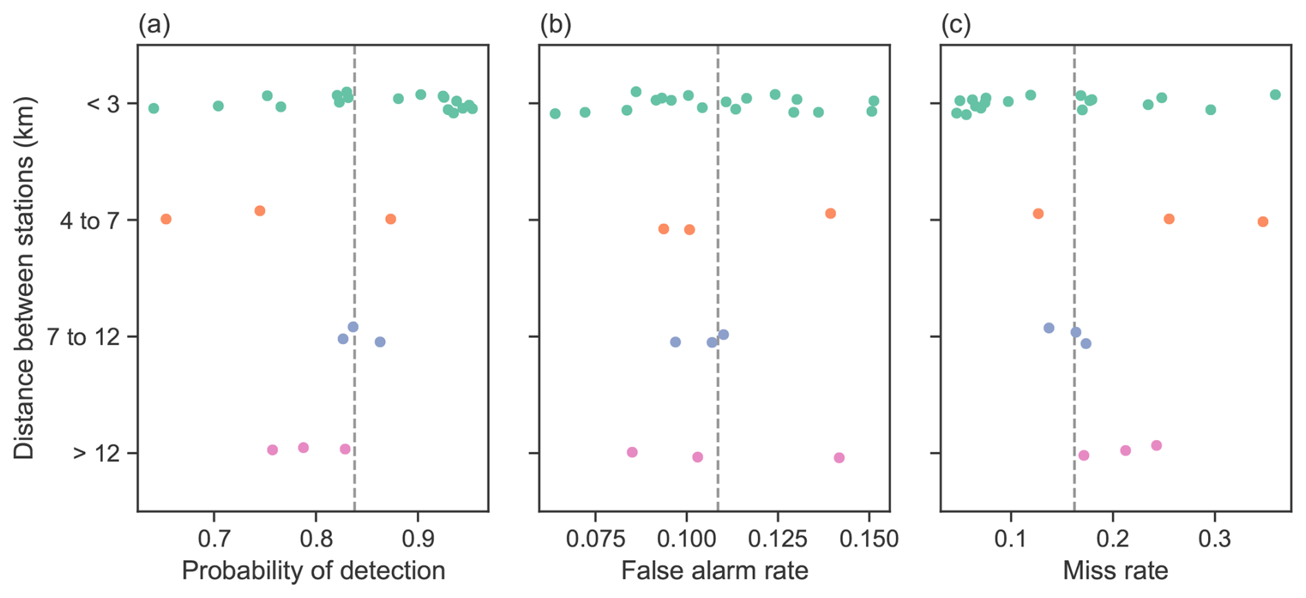
Figure 13 Comparison of the (a) probability of detection, (b) false-alarm rate, and (c) miss rate according to the distance between the study site and paired weather stations. The dashed grey line corresponds to the metric computed based on the full dataset in Fig. 12.

Figure 13 shows the variation of the instrument agreement according to the distance between stations. The station pairs are divided into four distance categories: less than 3 km, 4 to 7 km, 7 to 12 km, and more than 12 km. Generally, the stations separated by less than 3 km show better agreement, with a few outliers. However, the instrument agreement does not seem to decrease with distance as the 4 to 7 km category exhibits the poorest agreement. Notably, the Auxloups station, separated by 28 km from the nearest weather station, has a probability of detection of 0.79, a false-alarm rate of 0.14, and a miss rate of 0.21. These instrument agreement metrics are only slightly worse than the metrics of the 15 min dataset in Fig. 12. This suggests that instrument agreement is linked to site-specific conditions rather than to distance between stations. However, by discarding data points where the instruments do not agree, we ensure that precipitation events are consistent across study sites and weather stations. In addition, the coupling of instruments from nearby stations brings the spatial scale of the observational data closer to the scale of the reanalysis data.

Figure 14 Observed probability of occurrence for the solid, liquid, and mixed phases.

5.3 Data validation across studies

The phase observations from this study can be compared to other studies that use different validation data, such as direct observations (e.g. Behrangi et al., 2018; Dai, 2008; Jennings et al., 2018). However, it can be difficult to compare the phase occurrence according to the 2 m air temperature as the datasets in such studies often exclude mixed-phase precipitation. Consequently, the mixed phase is usually not analyzed in detail. One method to simply compare phase-partitioning models is the critical-threshold air temperature value CT_a, which is defined as the critical temperature threshold where both the solid and liquid phases have a 50 % chance of occurrence. In the case of this study, we define a different critical threshold for the solid phase (CT_S) and the liquid phase (CT_L), as well as a temperature where the probability for the mixed phase is highest (P_m). Figure 14 shows the probability of occurrence of the phases at the study sites separated into 0.2 °C bins. The resulting thresholds are CT_S of 1.3 °C, CT_L of 3.8 °C, and P_m of 2.4 °C for a mixed-phase probability of 0.44. It is also noteworthy that P_m is roughly where the probability of solid and liquid precipitation is equal. Because of this study's aggregation step, CT_S should be similar to CT_a values from other studies as the aggregation mostly affected the probability of mixed and liquid precipitation, and CT_L will be much warmer than CT_a.

In Behrangi et al. (2018), the average hourly CT_a of 1.58 °C aligns roughly with the study's CT_S and the calibrated 2 m air temperature threshold of the benchmark ST. One of the main conclusions from the study was that the wet-bulb temperature model is more robust than the dry-bulb temperature model as the CT_a can vary significantly from site to site. Humid conditions lead to a cooler CT_a, while drier conditions have the opposite effect. As such, the CT_a for humid conditions would be approximately equal to the mean value minus the standard deviation, resulting in 1.18 °C, and is thus closer to this study's CT_S of 1.3 °C. Additionally, the upper limit of CT_a of 2.16 °C in Behrangi et al. (2018) closely matches P_m. This finding lends credibility to the disdrometer phase identification and the phase aggregation step as it indicates the temperature range in which both solid and liquid phases are possible.

In Dai (2008), the overland 3-hourly CT_a of 1.2 °C is comparable to this study's CT_S despite the different time steps. The chance for the mixed phase in this study is much higher and more likely at warmer temperatures than in Dai (2008), where a peak 14.3 % chance of mixed rain and snow at 1.4 °C overland is reported. However, Ding et al. (2014) have shown that the probability of mixed-phase precipitation at the daily time step greatly increases under humid conditions, particularly near saturation. Such an analysis would, however, be required at the hourly time step to confirm this behaviour. The reasoning for the increase in mixed-phase precipitation probability is that the increase in relative humidity decreases evaporative cooling and favours a transition from snow to rain. In contrast, the temperature difference between the hydrometeors and the air decreases as humidity rises, which decreases sensible heat transfer and hinders the transition from snow to rain. The relatively homogenous conditions of the study sites could explain the differences in mixed-phase precipitation probability, while the analysis in Dai (2008) lumped together a large number of stations.

The findings in Jennings et al. (2018) show a much lower 3-hourly CT_a of 0.7 °C for precipitation in 90 %–100 % relative humidity and 0.9 °C for precipitation occurring in 90–105 kPa humidity and pressure conditions, under which the majority of this study's precipitation occurs. The greater difference between these CT_a and CT_S values could be due to several reasons. First, the 3-hourly CT_a should theoretically be lower than the hourly CT_a. As the time step increases, the occurrence of mixed-phase precipitation increases due to the higher likelihood of a phase transition. Second, the different types of validation data could explain why CT_a is generally lower than CT_S. Phase identification errors, particularly near the solid–liquid-phase transition, could also differ between direct observations and radar disdrometers.

Overall, the radar-based disdrometer measurements are similar to the findings of previous studies, although, generally, with slightly warmer conditions of occurrence for solid precipitation. However, more research is needed to properly quantify the uncertainties associated with this type of disdrometer. In addition, models based on automated phase observations may differ from those based on direct observations, especially as the time step can vary from study to study. This also highlights the importance of the verification step performed after aggregating mixed snow and rain or drizzle with rainfall as their effect was deemed to be closer to that of rainfall.

6 Conclusion

The study used phase measurements from radar-based disdrometers to train probabilistic models to classify and partition precipitation data for a network of study sites in eastern Canada. The study sites were located in predominantly boreal climates and at similar elevations, ranging from 315 to 641 m above sea level. The mean annual 2 m air temperature was around 0.2 °C, and the cumulative annual precipitation was significant at 902 mm. The humidity conditions for the data points used in the study were generally close to water vapour saturation. The utilization of automated measurements enabled partitioning of precipitation for mixed-phase events, which were previously limited to direct phase observations. The studied PGP models showed an improvement in phase partitioning with prior phase classification compared to benchmark models of varying complexity. PGP provides more accurate phase classification, which can benefit hydrological modelling at both local and watershed scales. It successfully reproduced the phase overlap between 1.5 and 3.5 °C, as seen in Fig. 7, where mixed-phase probability was the highest.

The classification performances show a substantial enhancement in phase classification as opposed to benchmark models, which were designed to minimize errors in phase partitioning. Additionally, the PGP models reduced partitioning error, especially PGP_hydromet and PGP_full. However, due to prior classification, partitioning performance is highly dependent on classification performance. As a result, the less complex PGP_basic had increased error variability. According to the input variable importance analysis, atmospheric pressure was the second most important near-surface variable for phase classification. The reanalysis atmospheric data reduced the partitioning error variability of PGP_full in comparison to the other PGP models. As for relative humidity, it was deemed to be the least important hydrometeorological feature for phase classification due to the regional homogeneity of the study sites. Overall, these findings demonstrate that automated phase observations enhance PGP method development and significantly improve precipitation phase classification, even with limited hydrometeorological information. The incorporation of reanalysis atmospheric data further enhances the accuracy of local observations, pointing toward potential operational applications for such methods.

The methodology of this study could be applied to other environments, including drier conditions or a broader spectrum of environments. Further research should include a comprehensive comparison of the radar-based disdrometers used in this study with other phase validation techniques to assess potential limitations. Research is also needed to improve the prediction of the mixed phase. Other variables such as wind speed could be considered as high wind speed can have a cooling effect on precipitation. Additionally, the impact of using a model that combines both phase classification and partitioning on snowpack accumulation and basin mass and energy dynamics should be investigated.

Appendix A: Study site details

Table A1 shows the details for the study sites used from the Hydro-Québec observational network.

Table A1 List of study site coordinates, elevations, and time frames for when the station was in operation.

Appendix B: Disdrometer phase identification validation

Snow water equivalent (SWE) and snow height observations were compiled from the entire network on a winter-by-winter basis. If more than 30 % of a winter's snowpack observations were missing at a station, that winter is not included in this analysis. The resulting data subset consists of 11 winter sites, with a total of 53 520 hourly data points. The hourly data were then separated into precipitation events. The following filters were applied to the events:

• duration ≥3 h

• mean 2 m air temperature between −5 and 5 °C

• total precipitation ≥0.5 mm

• mean SWE ≥15 mm.

This filtering step aimed to exclude short events and events that occurred either in warmer conditions, where phases other than rain are uncommon, or in the absence of snow cover detectable by the instrumentation in place. As such, 235 precipitation events were retained. In addition to the data points encompassing each event, the following hours were added until the next update of the SWE observations (at most 6 h). The events were then classified according to their main precipitation phase, i.e. the phase associated with at least half the total precipitation of the event.

Table B1 Precipitation event characteristics separated by phase.

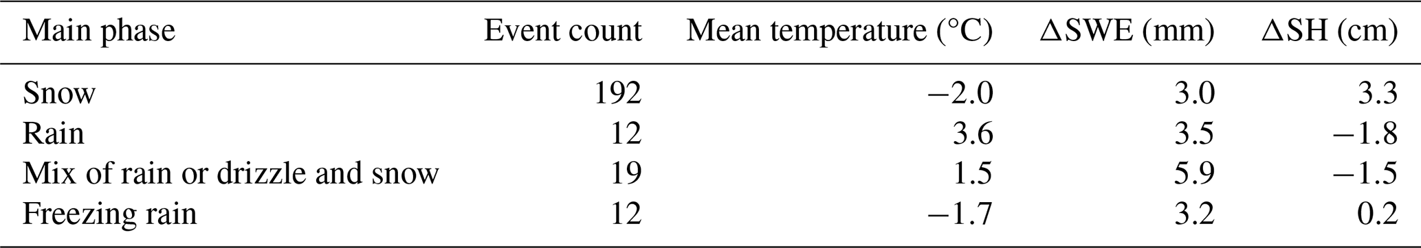
The mean 2 m air temperature, SWE variation (ΔSWE), and snow height variation (ΔSH) are compiled from precipitation events according to the main precipitation phase of the event (Table B1). The effects of rain and the mix of rain or drizzle and snow events on the snowpack are similar: an SWE increase accompanied by an SH decrease. In addition, the average temperature of mixed snow and rain or drizzle events is significantly above the freezing point, where rainfall is more likely to occur than snowfall. In the case of freezing rain, the average temperature during the events is more similar to snowfall. Although freezing rain does not generally increase the SH, it contributes to the solid component of the snowpack as it freezes on contact. Thus, the phase aggregation of this study was based on the hydrological impact and temperature range of freezing rain and the mix of rain or drizzle and snow.

Appendix C: Benchmark model description

The single-threshold model (ST) used to compute the solid-precipitation fraction f_snow (–) functions as follows:

$$\begin{array}{}\text{(C1)}& f_{\mathrm{snow}}=\left\{\begin{array}{ll}\mathrm{1}& T_{\mathrm{a}}\le T_K\\ \mathrm{0}& T_{\mathrm{a}}>T_K\end{array}\right.,\end{array}$$

where T_a is the temperature (°C), and T_K is the calibrated temperature threshold (°C). The linear-transition model (LT) uses two calibrated thresholds to calculate f_snow:

$$\begin{array}{}\text{(C2)}& f_{\mathrm{snow}}=\left\{\begin{array}{lll}\mathrm{1}& & T_{\mathrm{a}}\le T_{\mathrm{snow}}\\ \frac{T_{\mathrm{rain}}-T_{\mathrm{a}}}{T_{\mathrm{rain}}-T_{\mathrm{snow}}}& T_{\mathrm{snow}}<& T_{\mathrm{a}}<T_{\mathrm{rain}}\\ \mathrm{0}& & T_{\mathrm{a}}\ge T_{\mathrm{rain}}\end{array}\right.,\end{array}$$

where T_rain and T_snow are the calibrated rain and snow thresholds (°C). Finally, the psychrometric-energy-balance model (PB) (Harder and Pomeroy, 2013) calculates f_snow as follows:

$$\begin{array}{}\text{(C3)}& f_{\mathrm{snow}}={\displaystyle \frac{\mathrm{1}}{\mathrm{1}+b+c^{T_{\mathrm{i}}}}},\end{array}$$

where b and c are calibrated values, and T_i is the temperature of an unventilated hydrometeor (°C). Based on the mass balance of a sublimating ice sphere, T_i is calculated iteratively with the following function:

$$\begin{array}{}\text{(C4)}& T_{\mathrm{i}}=T_{\mathrm{a}}+L_t{\displaystyle \frac{D}{{\mathit{\lambda }}_t}}\left({\mathit{\rho }}_{T_{\mathrm{a}}}-{\mathit{\rho }}_{T_{\mathrm{i}}},\right)\end{array}$$

where L_t is the latent heat of sublimation or vaporization (J k⁻¹); D is the diffusivity of water vapour (m² s⁻¹); λ_t is the thermal conductivity of air (J m⁻¹ s⁻¹ K⁻¹); and ${\mathit{\rho }}_{T_{\mathrm{a}}}$ and ${\mathit{\rho }}_{T_{\mathrm{i}}}$ are the water vapour density of the surrounding air and on the hydrometeor's surface, respectively (kg m⁻³). The procedure to compute the variables is as detailed in Harder and Pomeroy (2013). D is computed following Thorpe and Mason (1966):

$$\begin{array}{}\text{(C5)}& D=\mathrm{2.06}\times {\mathrm{10}}^{-\mathrm{5}}{\left({\displaystyle \frac{T_{\mathrm{a}}}{\mathrm{273.15}}}\right)}^{\mathrm{1.75}}.\end{array}$$

The vapour pressure e (kPa) is computed as in Dingman (2015):

$$\begin{array}{}\text{(C6)}& e={\displaystyle \frac{\text{RH}}{\mathrm{100}}}\times \mathrm{0.611}\exp \left({\displaystyle \frac{\mathrm{17.37}T}{\mathrm{237.3}+T}}\right),\end{array}$$

where RH is the relative humidity (%), and T is the air temperature (°C). ρ is computed following the ideal gas law:

$$\begin{array}{}\text{(C7)}& \mathit{\rho }={\displaystyle \frac{m_{\mathrm{w}}e}{RT}},\end{array}$$

where m_w is the molecular weight of water (0.01801528 kg mol⁻¹), and R is the universal gas constant (8.31441 J mol⁻¹ K⁻¹). The air thermal conductivity λ_t is computed as in List (1951):

$$\begin{array}{}\text{(C8)}& {\mathit{\lambda }}_t=\mathrm{0.000063}{T}_{\mathrm{a}}+\mathrm{0.00673}.\end{array}$$

Finally, the latent heat of sublimation (T_a<0) and vaporization (T_a≥0) is computed as follows (Yau and Rogers, 1996):

$$\begin{array}{}\text{(C9)}& L_t=\left\{\begin{array}{ll}\mathrm{1000}(\mathrm{2834.1}-\mathrm{0.29}{T}_{\mathrm{a}}-\mathrm{0.004}{T}_{\mathrm{a}}^{\mathrm{2}})& T_{\mathrm{a}}<\mathrm{0}\\ \mathrm{1000}(\mathrm{2501}-\mathrm{2.31}{T}_{\mathrm{a}}& T_{\mathrm{a}}\ge \mathrm{0}\end{array}\right.,\end{array}$$

Table C1 shows the calibrated parameters for the models presented in this section. The calibration was made on the same training set used for the PGP models. Figure C1 shows the simulated solid fraction for the benchmark models, as well as the observed solid fraction.

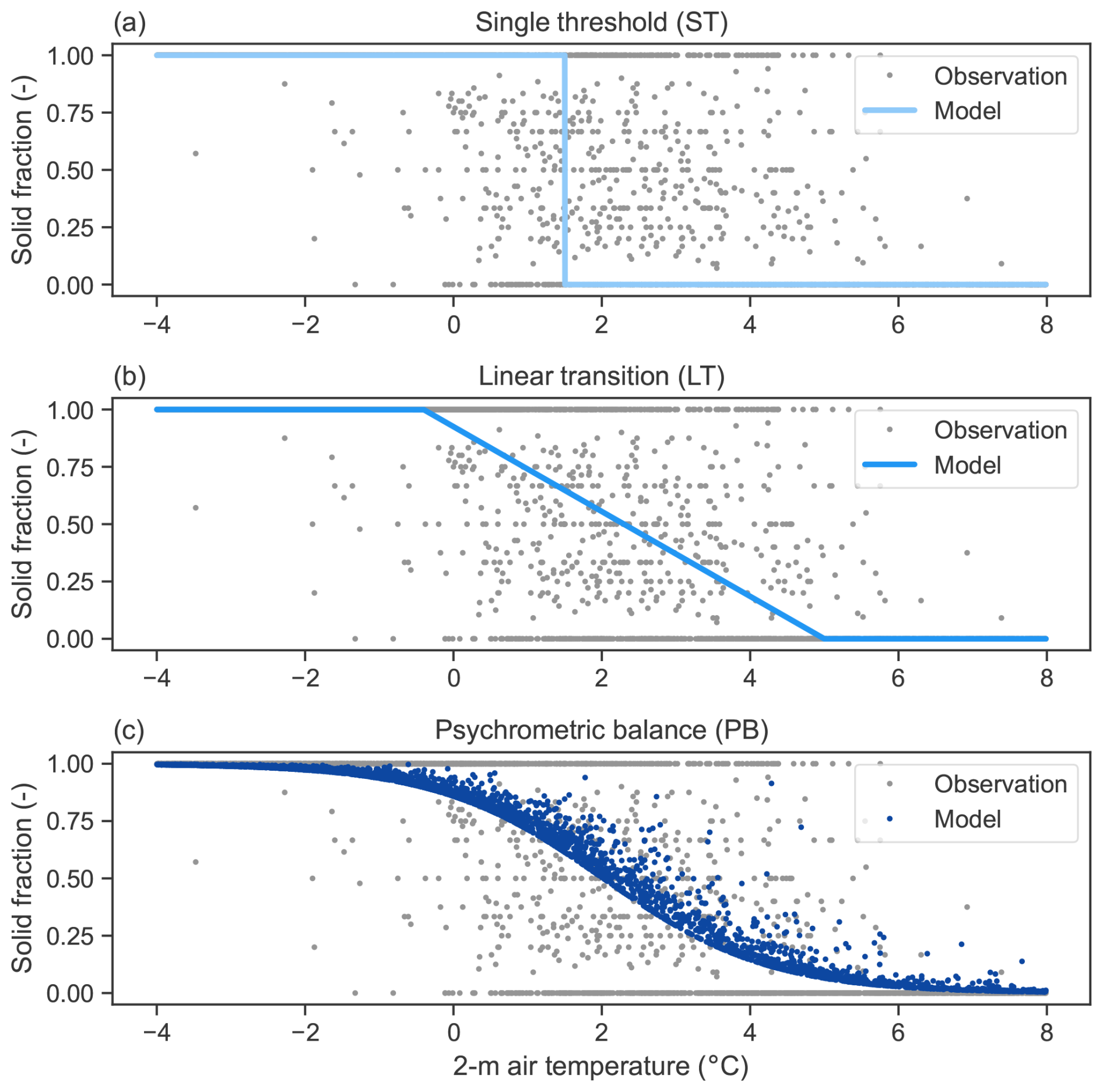
Figure C1 Observed solid-precipitation fraction according to the 2 m air temperature and the modelled solid-precipitation fraction of the (a) static threshold, (b) linear transition, and (c) psychrometric balance.

Table C1 Benchmark model calibrated parameters.