Technical Note: Revisiting the general calibration of cosmic-ray neutron sensors to estimate soil water content

Cosmic-ray neutron sensing (CRNS) is becoming increasingly popular for monitoring soil water content (SWC). To retrieve SWC from observed neutron intensities, local measurements of SWC are typically required to calibrate a location-specific parameter, N₀, in the corresponding transfer function. In this study, we develop a generalized conversion function that explicitly takes into account the different factors that govern local neutron intensity. Thus, the parameter N₀ becomes location independent, i.e. generally applicable. We demonstrate the feasibility of such a “general calibration function” by analysing 75 CRNS sites from four recently published datasets. Given the choice between the two calibration strategies – local or general – users will wonder which one is preferable. To answer this question, we estimated the resulting uncertainty in the SWC by means of error propagation. While the uncertainty in the local calibration depends on both the local reference SWC itself and its error, the uncertainty in the general calibration is mainly governed by the errors in vegetation biomass and soil bulk density. Our results suggest that a local calibration – generally considered best practice – might often not be the best option. In order to support the decision which calibration strategy – local or general – is actually preferable in the user-specific application context, we provide an interactive online tool that assesses the uncertainty in both options (https://cosmic-sense.github.io/local-or-global, last access: 23 February 2024).

1 Introduction

Cosmic-ray neutron sensing (CRNS) is becoming increasingly popular for monitoring soil water content (SWC). The technology is non-invasive and has a horizontal footprint of around 150 m together with a vertical penetration depth of typically up to 30 cm. Thus, CRNS overcomes a fundamental disadvantage of point measurements – the lack of spatial representativeness.

Yet, the estimation of volumetric soil water content (θ, in m³ m⁻³) from observed neutron count rates (N, in counts per hour, cph) requires reference measurements of θ in order to calibrate the parameter N₀ in the functional relationship proposed by Desilets et al. (2010):

$$\begin{array}{}\text{(1)}& \mathit{\theta }\left(N\right)=\left({\displaystyle \frac{a_{\mathrm{0}}}{\frac{N}{N_{\mathrm{0}}}-a_{\mathrm{1}}}}-a_{\mathrm{2}}\right)\cdot {\displaystyle \frac{{\mathit{\rho }}_{\mathrm{b}}}{{\mathit{\rho }}_{\mathrm{w}}}},\end{array}$$

where ρ_b is the soil bulk density (kg m⁻³), ρ_w is the density of water (kg m⁻³), and a₀=0.0808, a₁=0.372, and a₂=0.115 are constants.

Typically, such reference measurements of θ_cal consist of 10–20 profiles in the CRNS footprint: within the upper 30 cm of the soil, θ and ρ_b are measured at different depth increments and within various distances from the neutron detector. In order to obtain a value of θ_cal that is representative for the detector footprint, the individual measurements at different depths and horizontal distances are averaged by a set of weighting functions (Schrön et al., 2017).

These reference measurements are labour intensive (roughly one person-day for sampling only, excluding travels and laboratory analysis). More importantly, though, the variability in θ at different spatial scales makes it difficult to representatively cover a circle of 150 m radius with such a limited number of samples. Any error in θ_cal is expected to propagate to θ(N), although systematic studies to that effect, to our knowledge, do not yet exist.

For mobile applications (CRNS roving), e.g. by car (Schrön et al., 2018b) or train (Altdorff et al., 2023), the problem becomes even more obvious as obtaining reference measurements along extended roving tracks is practically impossible. Other conditions can make reference measurements difficult to unfeasible, such as access restrictions (e.g. to agricultural fields, private property) or soil properties (stones, roots).

Ideally, the local calibration of N₀ could be replaced by a general relationship which takes into account all the factors (apart from SWC) that influence the local neutron intensity and hence any estimate of N₀. The key ingredients for such a relationship were elaborated in this journal about 11 years ago. Zreda et al. (2012) outlined a framework for the COSMOS network to account for

• the dynamic effects of barometric pressure, air humidity, and the incoming neutron flux (for which the correction functions are still commonly used, although alternatives were suggested);

• the spatial variation in incoming cosmic-ray secondary neutron intensity as governed by the Earth's geomagnetic field and the location in the atmosphere (i.e. altitude), based on a model proposed by Desilets and Zreda (2003);

• the efficiency of the neutron detector, by defining a reference probe (the first COSMOS site in San Pedro) to which all neutron count rates could be scaled.

This concept was further refined by Franz et al. (2013), again in this journal, who suggested a “universal calibration function for determination of soil moisture with cosmic-ray neutrons” to take into account the differences in various hydrogen pools between different sites, namely biomass, soil organic matter (OM), and lattice water (LW). Based on the data from 35 COSMOS sites and 45 calibration dates, Franz et al. (2013) demonstrated the basic feasibility of the concept, although it should be noted that the functional relationship was formally established between neutron intensity and the molar fraction of hydrogen in a support volume (instead of θ). The authors also suggested a detector-specific calibration parameter, N_s, which represents the neutron count rate over water. This concept has been tested by McJannet et al. (2014), Baatz et al. (2014) and Iwema et al. (2015) at different sites, but a general improvement in performance for quantifying soil moisture was not confirmed.

Recently, in this journal, Heistermann et al. (2021) demonstrated the feasibility of what they referred to as the estimation of a “single N₀”. For this purpose, they used 18 CRNS sensors that were distributed as a cluster in an area of 1 km² in a pre-Alpine catchment in Germany (Fersch et al., 2020). The study area was characterized by substantial landscape heterogeneity, including grassland and mature forests, mineral and peat soils, and locations close to and distant from the groundwater table. Within that 1 km², it was possible to use a single value of N₀ after the effects of different sensor sensitivities as well as hydrogen pools (biomass, soil organic matter, lattice water) were carefully accounted for. As for hydrogen pools, obviously, the difference between forest (above-ground dry biomass around 24 kg m⁻²) and grassland (around 0.2 kg m⁻²) was a dominant factor.

In this paper, we would like to revisit the idea of a general functional relationship as suggested by Zreda et al. (2012) and Franz et al. (2013). This requires the user to account for the relative sensitivity of the neutron detector, the effects of other hydrogen pools in the sensor footprint, and the effects of geographic latitude, longitude, and altitude. To that end, we build upon Eq. (1) and combine it with well-established functional relationships and models, as outlined in Sect. 3. We then use four recently published CRNS datasets in order to estimate a single value of N₀ to be applied across all sensors.

Yet, we would like to go one step further. While Franz et al. (2013) saw the value of a “universal calibration function” rather for situations in which reference measurements of θ were unfeasible, we would like to ask whether omitting a local calibration could be an opportunity to avoid a fundamental source of uncertainty: the reference measurement of θ_cal. In order to answer this question, we analyse the propagation of errors for two contrasting calibration scenarios, local and general. Based on this uncertainty analysis, we will outline typical constellations under which one or the other option would be preferable, and give a rough assessment of the dominant sources of uncertainty.

2 Data

Recently, four major European CRNS datasets were published in the Copernicus journal Earth System Science Data.

In the COSMOS-Europe dataset, Bogena et al. (2022) compiled neutron counts data and reference observations of θ_cal as well as other variables (such as bulk density, soil organic carbon, lattice water, barometric pressure, air humidity, and temperature) for 66 CRNS stations from 24 research institutions across Europe.

Moreover, three dedicated field campaigns were carried out by the Cosmic Sense research unit, a consortium of eight research institutions funded by the German Research Foundation (DFG). These campaigns all had in common the concept of dense CRNS clusters, meaning that a relatively large number of CRNS detectors (8–18) was operated within a relatively small area (0.1–1 km²). All three campaigns included extensive soil sampling to obtain reference measurements of θ_cal but also soil bulk density, soil organic matter content, lattice water, and above-ground biomass for forested and non-forested areas. We will refer to each of these datasets by the location of the campaign.

• Fendt: Fersch et al. (2020) published the results of a large campaign from May to July 2019 during which 18 CRNS detectors were continuously operated as a cluster within an area of 1 km², in the pre-Alpine upper Rott catchment in southern Germany. It is this dataset for which Heistermann et al. (2021) had demonstrated the feasibility of estimating one single N₀ for a large set of CRNS footprints.

• Wüstebach: a similar campaign with 15 CRNS was carried out from September to November 2020 in the 0.4 km² Wüstebach catchment (Eifel mountains in western Germany), which is governed by a mature spruce forest, together with a significant clear-cut area, at altitudes between 595 and 628 m (Heistermann et al., 2022).

• Marquardt: recently, Heistermann et al. (2023a) published a dataset of eight CRNS per 0.1 km² that were operated over a period of 3 years in an agricultural research site in the lowlands of north-east Germany.

The four datasets are publicly available and comprehensively documented in the above references. Together, they include a total of 107 CRNS stations. An important feature of this combined dataset is that it covers different spatial scales: while the COSMOS-Europe dataset extends over Europe, the three dense CRNS clusters are distributed across Germany and each of them, in turn, covers substantial heterogeneity at extents between 0.1 and 1 km². At these different scales (continental to local), different factors are expected to govern the variability in neutron intensity: while the effect of the geomagnetic field might be important at the continental scale, the effect of altitude might play a role at the regional scale, whereas the heterogeneity of the landscape with regard to different hydrogen pools might be dominant at the field or small catchment scale.

3 Methods

3.1 A general function for θ(N)

The proposed general function for θ^G(N) builds on well-established community standards. In essence, we introduce various terms to Eq. (1) which take into account the previously mentioned effects on epithermal neutron intensity. These terms either multiplicatively scale the observed neutron intensity or additively represent other hydrogen pools as equivalents of soil water. The resulting equation corresponds to Eq. (1) in Power et al. (2021), supplemented by the correction factor f_s:

$$\begin{array}{}\text{(2)}& \begin{array}{rl}{\mathit{\theta }}^{\mathrm{G}}\left(N\right)& =\left({\displaystyle \frac{a_{\mathrm{0}}}{f_{\mathrm{p}}\cdot f_{\mathrm{h}}\cdot f_{\mathrm{in}}\cdot f_{\mathrm{b}}\cdot f_{\mathrm{s}}\cdot \frac{N}{N_{\mathrm{0}}}-a_{\mathrm{1}}}}-a_{\mathrm{2}}-{\mathit{\theta }}_{\mathrm{g}}^{\mathrm{OM}}\right.\\ & \left.-{\mathit{\theta }}_{\mathrm{g}}^{\mathrm{LW}}\right)\cdot {\displaystyle \frac{{\mathit{\rho }}_{\mathrm{b}}}{{\mathit{\rho }}_{\mathrm{w}}}}.\end{array}\end{array}$$

The dimensionless multiplicative scaling factors of f represent the effects of barometric pressure (f_p), air humidity (f_h), incoming neutron intensity (f_in), vegetation biomass (f_b), and detector sensitivity (f_s). ${\mathit{\theta }}_{\mathrm{g}}^{\mathrm{OM}}$ and ${\mathit{\theta }}_{\mathrm{g}}^{\mathrm{LW}}$ are the equivalents of gravimetric soil water content resulting from soil organic matter and lattice water respectively (in g g⁻¹).

If we assume that Eq. (2) represents all relevant processes that affect the relationship between θ and N, the parameter N₀ should be the same in any location which meets this assumption (note that, in this study, we do not account for the presence of snow or for topographic shielding of cosmogenic neutrons in locations with complex and steep topography; see, e.g. Dunne et al., 1999; Balco, 2014; Schattan et al., 2019). The various components of Eq. (2) are detailed in the following:

$$\begin{array}{}\text{(3)}& f_{\mathrm{p}}=f_{\mathrm{p}}\left(p\right)=\exp \left({\displaystyle \frac{p-p_{\mathrm{0}}}{L}}\right).\end{array}$$

f_p was suggested by Zreda et al. (2012) and accounts for the effects of barometric pressure variations over time (p, in g cm⁻²: barometric pressure at the time of the neutron measurement; p₀, in g cm⁻²: arbitrary reference pressure, e.g. the long-term average of p at the measurement site or the standard pressure at the altitude of the station; L, in g cm⁻²: mass attenuation length for high-energy neutrons, set to a constant value of 131.6 g cm⁻²). In theory, L depends on the geomagnetic location but Bogena et al. (2022) found no significant variation across Europe. In this study, we assume that any remaining effects of cut-off rigidity will be accounted for by the correction function f_in (see Eq. 5).

$$\begin{array}{}\text{(4)}& f_{\mathrm{h}}=f_{\mathrm{h}}\left(h\right)=\mathrm{1}+\mathit{\alpha }\cdot \left(h-h_{\mathrm{0}}\right)\end{array}$$

Rosolem et al. (2013) suggested f_h in order to account for the temporal variation in the absolute humidity of the air (h, in g m⁻³) from an arbitrary reference h₀ (here the temporal average of h at the measurement site in Marquardt, yielding h₀=7.5 g m⁻³) and determined the value of α as 0.0054 m³ g⁻¹ by means of neutron simulations.

$$\begin{array}{}\text{(5)}& \begin{array}{rl}{f}_{\mathrm{in}}=& f_{\mathrm{in}}(\mathit{\varphi },\mathit{\lambda },z,I)=f_{\mathrm{in}}^{\mathrm{t}}\left(I\right)\cdot f_{\mathrm{in}}^{\mathrm{s}}(\mathit{\varphi },\mathit{\lambda },z)\mathrm{with}\\ & f_{\mathrm{in}}^{\mathrm{t}}\left(I\right)={\displaystyle \frac{I_{\mathrm{0}}}{I}},f_{\mathrm{in}}^{\mathrm{s}}(\mathit{\varphi },\mathit{\lambda },z)={\displaystyle \frac{\mathit{\xi }\left({\mathit{\varphi }}_{\mathrm{0}},{\mathit{\lambda }}_{\mathrm{0}},z_{\mathrm{0}}\right)}{\mathit{\xi }(\mathit{\varphi },\mathit{\lambda },z)}}\end{array}\end{array}$$

f_in accounts for the temporal ($f_{\mathrm{in}}^{\mathrm{t}}$) and spatial ($f_{\mathrm{in}}^{\mathrm{s}}$) variation in incoming high-energy neutrons. Typically, CRNS-related studies only consider $f_{\mathrm{in}}^{\mathrm{t}}$ by relating the secondary neutron intensity I (in cph) observed by one of the monitors in the neutron monitor database (NMDB) to an arbitrary reference intensity I₀ (here the average of I at the monitor between 2009 and 2023). For most CRNS applications in Europe, the neutron monitor at Jungfraujoch (“JUNG” in the NMDB) is chosen for that purpose, and we do the same in this study.

The spatial variation $f_{\mathrm{in}}^{\mathrm{s}}$ of incoming neutrons is typically not considered, but for a general relationship θ(N), it becomes crucial. $f_{\mathrm{in}}^{\mathrm{s}}$ is a function of the geomagnetic field of the Earth (which varies with longitude λ and latitude ϕ, both in decimal degrees) and the attenuation by the atmosphere which, in turn, is a function of altitude (z, in m a.s.l.). For this study, we use the PARMA model (Sato, 2015) to simulate $f_{\mathrm{in}}^{\mathrm{s}}$ in a consistent way. While the PARMA model covers a wide range of particles and energy levels, the value $\mathit{\xi }(\mathit{\lambda },\mathit{\varphi },z)$ in Eq. (5) corresponds to the average of simulated neutron intensities at energies from 1 to 10⁵ eV. Thus, we directly represent the effect of location (λ, ϕ, z) on the average epithermal neutron intensity. Although the PARMA model is able to account for some aspects of the temporal variation in incoming neutrons (e.g. solar cycles), we use an arbitrary reference date (31 May 2019) as input since the temporal variation in incoming neutron intensity across various timescales is represented by $f_{\mathrm{in}}^{\mathrm{t}}$. In order to obtain a scaling factor $f_{\mathrm{in}}^{\mathrm{s}}$, we scale ξ at any location (λ, ϕ, z) by ξ at an arbitrary location (defined by λ₀=12.97°, ϕ₀=52.47°, and z₀=40 m). This arbitrary location corresponds to the research site in Marquardt (about 10 km south-west of Berlin, Germany; see Heistermann et al., 2023a).

$$\begin{array}{}\text{(6)}& f_{\mathrm{b}}\left(t\right)={\displaystyle \frac{\mathrm{1}}{\mathrm{1}-\mathrm{0.009}\cdot \mathrm{AGB}}}\end{array}$$

f_b accounts for the effect of vegetation biomass on neutron count rates. The equation is based on the empirical analysis of a wide range of biomass levels by Baatz et al. (2015), according to which epithermal neutron count rates are reduced by 0.9 % for every kilogram of dry above-ground biomass per m² (AGB). This rate is similar to the reduction of 1 % per kg m⁻² reported by Franz et al. (2015) for croplands. It should be noted that, based on neutron transport modelling, Andreasen et al. (2017, 2020) found an effect of forest canopy structure on the reduction in epithermal neutron intensity. Apart from this effect of canopy structure, it also remains an open issue as to which extent simple linear reduction rates may apply for very high biomass levels.

$$\begin{array}{}\text{(7)}& f_{\mathrm{s}}={\displaystyle \frac{N_{\mathrm{ref}}}{N}}\end{array}$$

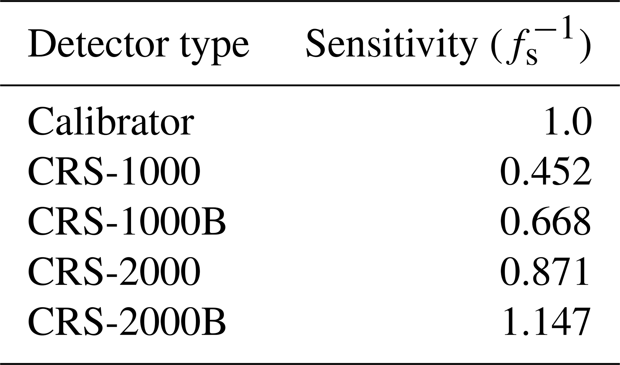
The sensitivity factor f_s accounts for the detector efficiency and is used to scale observed neutron intensities N to the intensity N_ref that would have been observed by an arbitrary reference detector. For our reference detector, we chose a so-called “calibrator” probe (manufactured by Hydroinnova, two counter tubes based on ³He gas). During the above-mentioned campaigns in Fendt, Wüstebach, and Marquardt, we collocated such a calibrator with various types of CRNS sensors over longer periods (typically several days) in order to obtain f_s. For sensors which are missing a calibrator collocation (most sensors in the COSMOS-Europe dataset, a few sensors in the other three datasets), we assumed the average value of f_s for the corresponding detector type (see Table 1). However, one should keep in mind that sensitivity might slightly vary between instruments of the same type (Schrön et al., 2018a, found variations of 1 %–3 % in an intercomparison study that included nine CRS-1000 instruments). Another way to replace a calibrator measurement is to collocate a sensor with another sensor for which f_s is known (“cross-calibration”). In the case neither a direct reference measurement nor an average f_s for a detector type nor cross-calibration is an option, f_s remains unknown and Eq. (2) cannot be applied. While this applies to any variable in Eq. (2) required for the general calibration strategy, the quantification of f_s might constitute a particular challenge in the case a suitable reference is unavailable to the user, e.g. when a new type or brand of CRNS detector is introduced. Within the set of 107 CRNS sensors from our four datasets, we were able to retrieve f_s for 100 locations.

$$\begin{array}{}\text{(8)}& {\mathit{\theta }}_{\mathrm{g}}^{\mathrm{OM}}=\mathrm{0.556}\cdot \mathrm{OM}\end{array}$$

Following McJannet et al. (2014), ${\mathit{\theta }}_{\mathrm{g}}^{\mathrm{OM}}$ is 0.556 times the organic matter content (OM, g g⁻¹), based on the stoichiometry of cellulose. Finally, ${\mathit{\theta }}_{\mathrm{g}}^{\mathrm{LW}}$ can be taken directly from measurements.

Table 1 Average detector efficiencies (sensitivities) observed for the most common detector models, all from Hydroinnova Ltd, USA (94 out of the 107 detectors in the combined dataset are of one of these types). Note that the sensitivity column shows the inverse of f_s: the lower the count efficiency of the detector, the higher the value of f_s.

3.2 Data filtering and processing

For the estimation of N₀ in Eq. (2), we discarded a number of CRNS locations and calibration dates from the COSMOS-Europe dataset, namely locations or calibration dates for which

• the sensitivity factor f_s was unknown and could not be inferred from the sensor type;

• the soil sampling data for calibration were insufficient (e.g. less than 18 profiles, only surface sampling, missing bulk density);

• the sensor was placed in or close to a forest but no biomass estimates were available to us (which effectively applies to most forest locations in the COSMOS-Europe dataset).

From the COSMOS-Europe location with ID JEC001 (Jena), we randomly selected 4 out of a total of 30 calibration dates in order to avoid the location being over-represented in the calibration dataset.

After filtering, 75 CRNS locations with a total of 104 calibration dates were still available for analysis. Based on the published datasets, we derived the required parameters of Eq. (2) for each location and calibration date. For bulk density, soil organic matter content, lattice water, above-ground dry biomass, and volumetric soil moisture, we obtained weighted average values by applying the weighting function provided by Schrön et al. (2017).

3.3 Error propagation

As pointed out in the introduction, we aim to compare two contrasting application scenarios with regard to the resulting uncertainty for θ(N):

1. the use of a general calibration of θ^G(N), Eq. (2), for which we need to determine a wide range of location-specific parameters but can estimate and then apply a location-independent estimate of N₀;

2. the local calibration of N₀ in Eq. (1), for which we require a local reference measurement of θ_cal and an estimate of the soil bulk density ρ_b within the sensor footprint.

Assuming independent variables and normally distributed errors, we can apply Gaussian error propagation for both scenarios. This approach has been followed by other studies on neutron counts (Weimar et al., 2020; Schrön et al., 2021), on neutrons and bulk density (Jakobi et al., 2020), and on neutrons, N₀, meteorological parameters, and sampling tube geometries (Gugerli et al., 2019).

For the general calibration, the uncertainty in θ^G(N) is obtained by propagating the errors in the following variables: the sensitivity factor f_s, the observed neutron intensity N, the estimated value of N₀, the above-ground dry biomass AGB, the organic matter content OM, the lattice water content θ_LW, and the soil bulk density ρ_b. For the sake of simplicity, the effects of the correction factors f_p, f_h, and f_in are not included: the underlying measurement uncertainties in pressure, humidity, and incoming neutron intensity at Jungfraujoch are considered relatively small, while the uncertainty in $f_{\mathrm{in}}^{\mathrm{s}}$ as derived from the PARMA model is difficult to quantify. Moreover, f_p, f_h, and f_in would be applied in the local calibration scenario, too, so both scenarios were similarly affected.

In summary, the following equation describes the uncertainty in θ^G(N) in terms of its standard deviation ${\mathit{\sigma }}_{{\mathit{\theta }}^{\mathrm{G}}}$ (in m³ m⁻³):

$$\begin{array}{}\text{(9)}& \begin{array}{rl}{\mathit{\sigma }}_{{\mathit{\theta }}^{\mathrm{G}}}=& \sqrt{\sum _x{\left({\displaystyle \frac{\partial {\mathit{\theta }}_{\mathrm{G}}}{\partial x}}\right)}^{\mathrm{2}}{\mathit{\sigma }}_x^{\mathrm{2}}}\mathrm{for}x\in \left\{f_{\mathrm{s}},\mathrm{AGB},N,N_{\mathrm{0}},\mathrm{OM},\right.\\ & \left.{\mathit{\theta }}_{\mathrm{LW}},{\mathit{\rho }}_{\mathrm{b}}\right\},\end{array}\end{array}$$

where all σ denote the error in the respective variable x.

For the error propagation in the local calibration scenario, we used Eq. (1) to derive an expression, θ^L(N), which provides the CRNS-based SWC as a function of the local calibration measurements (N_cal, θ_cal) and of the observed neutron intensity N at any point in time. For this purpose, we first insert N_cal and θ_cal into Eq. (1), solve for N₀ (i.e. calibrating the local N₀), and then insert the resulting term again to Eq. (1) (i.e. applying the locally calibrated N₀).

Typically, the neutron intensities N and N_cal are corrected for the temporal variation in pressure, humidity, and incoming neutrons. We summarize these correction factors as $\mathit{\tau }=f_{\mathrm{p}}\cdot f_{\mathrm{h}}\cdot f_{\mathrm{in}}$ which corresponds to the period during which N was observed, while τ_cal is the corresponding correction factor for N_cal. Altogether, we obtain

$$\begin{array}{}\text{(10)}& \begin{array}{rl}{\mathit{\theta }}^{\mathrm{L}}\left(N\right)& =(a_{\mathrm{0}}\cdot ({\displaystyle \frac{\mathit{\tau }\cdot N}{{\mathit{\tau }}_{\mathrm{cal}}}}\cdot N_{\mathrm{cal}}\cdot ({\displaystyle \frac{a_{\mathrm{0}}}{{\mathit{\theta }}_{\mathrm{cal}}\cdot \frac{{\mathit{\rho }}_{\mathrm{w}}}{{\mathit{\rho }}_{\mathrm{b}}}+a_{\mathrm{2}}}}\\ & +a_{\mathrm{1}})-a_{\mathrm{1}}{)}^{-\mathrm{1}}-a_{\mathrm{2}})\cdot {\displaystyle \frac{{\mathit{\rho }}_{\mathrm{b}}}{{\mathit{\rho }}_{\mathrm{w}}}}.\end{array}\end{array}$$

We then propagated the errors in N, N_cal, θ_cal, and ρ_b to θ^L(N) to obtain the corresponding error ${\mathit{\sigma }}_{{\mathit{\theta }}^{\mathrm{L}}}$ (in m³ m⁻³), while neglecting the errors in f_p, f_h, and f_in as explained above:

$$\begin{array}{}\text{(11)}& {\mathit{\sigma }}_{{\mathit{\theta }}^{\mathrm{L}}}=\sqrt{{{\displaystyle \frac{\partial {\mathit{\theta }}^{\mathrm{L}}}{\partial N}}}^{\mathrm{2}}{\mathit{\sigma }}_N^{\mathrm{2}}+{{\displaystyle \frac{\partial {\mathit{\theta }}^{\mathrm{L}}}{\partial N_{\mathrm{cal}}}}}^{\mathrm{2}}{\mathit{\sigma }}_{N_{\mathrm{cal}}}^{\mathrm{2}}+{{\displaystyle \frac{\partial {\mathit{\theta }}^{\mathrm{L}}}{\partial {\mathit{\theta }}_{\mathrm{cal}}}}}^{\mathrm{2}}{\mathit{\sigma }}_{{\mathit{\theta }}_{\mathrm{cal}}}^{\mathrm{2}}+{{\displaystyle \frac{\partial {\mathit{\theta }}^{\mathrm{L}}}{\partial {\mathit{\rho }}_{\mathrm{b}}}}}^{\mathrm{2}}{\mathit{\sigma }}_{{\mathit{\rho }}_{\mathrm{b}}}^{\mathrm{2}}}.\end{array}$$

For the local calibration scenario, it could also be an option to use Eq. (2) instead of the simplified Eq. (1). This would require quantifying all parameters as precisely as possible (particularly the additive offsets ${\mathit{\theta }}_{\mathrm{OM}}^{\mathrm{g}}$ and ${\mathit{\theta }}_{\mathrm{LW}}^{\mathrm{g}}$) and eventually estimating the local N₀. Ideally, this approach would make estimates of N₀ more consistent between different locations, corresponding to an intermediate between the local and the general calibration strategy. In our study, however, we decided to limit the analysis to a “purely local” approach, where the simpler Eq. (1) is used in order to avoid the introduction of additional sources of uncertainty. The strength of this approach is that the uncertainties in all other parameters could be effectively lumped into the estimation of N₀. Future uncertainty analyses, however, might decide to include at least the offset terms ${\mathit{\theta }}_{\mathrm{OM}}^{\mathrm{g}}$ and ${\mathit{\theta }}_{\mathrm{LW}}^{\mathrm{g}}$ in the evaluation of the local calibration approach.

The required partial derivatives of θ^G and θ^L are provided in the supplementary to this technical note.

4 Results and discussion

4.1 A general function for θ(N)

As pointed out in Sect. 3.2, a total of 75 CRNS locations and 104 calibration dates remained after applying a set of filtering rules. Based on this subset, N₀ in Eq. (2) was determined by minimizing the mean absolute error (MAE) between θ^G(N_cal) and θ_cal, yielding N₀=2306 cph and MAE = 0.075 m³ m⁻³. Note that this value of N₀ has no fundamental physical meaning; it is a result of our general calibration framework in which all neutron count rates are scaled to arbitrary references for sensitivity (Hydroinnova's calibrator), geographic location (Marquardt), and conditions without vegetation. Figure 1 illustrates the calibration results.

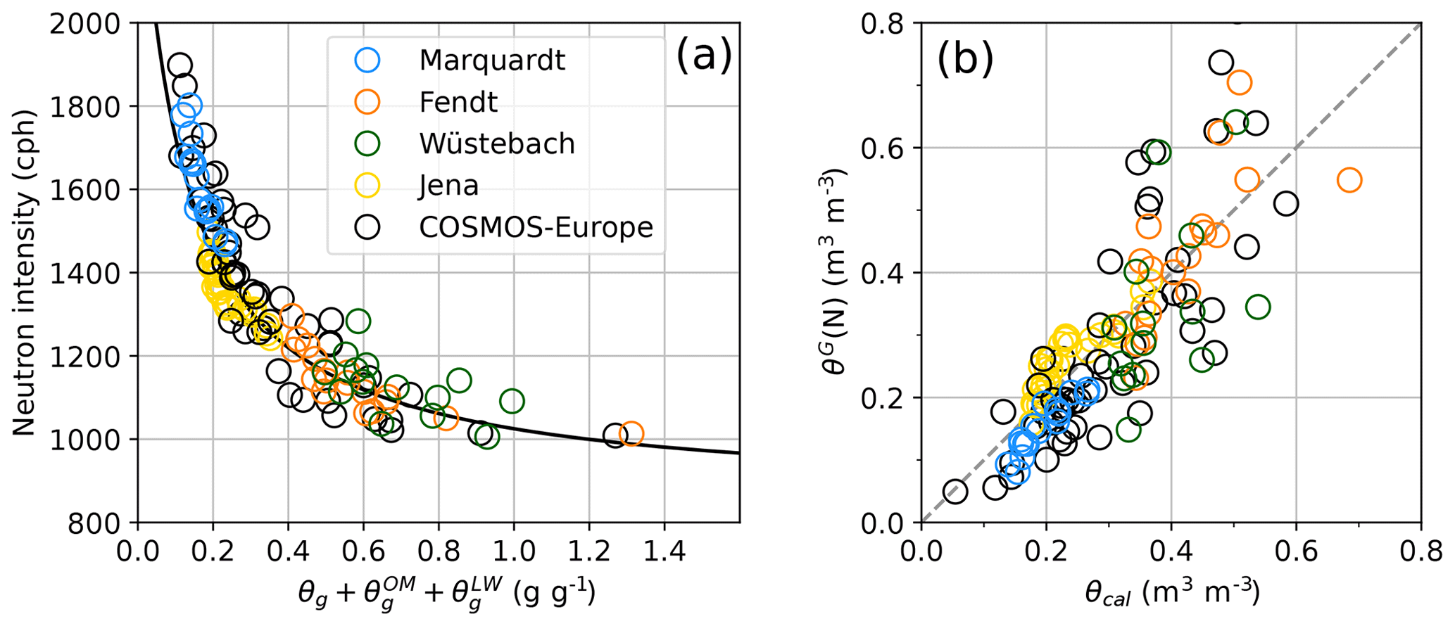
Figure 1 (a) Scaled neutron intensity (all multiplicative factors f in Eq. 2 applied) plotted over “apparent gravimetric SWC”, i.e. the sum of gravimetric SWC and the equivalents of SWC resulting from soil organic matter and lattice water. The line shows Eq. (2), solved for the scaled neutron intensity. (b) θ^G(N) (i.e. CRNS-based estimate of SWC) over θ_cal (i.e. SWC obtained from soil sampling) for all analysed CRNS locations and calibration dates. For Jena (location JEC001 in COSMOS-Europe), we show the estimates for all available calibration dates not only the four selected for calibration.

Figure 1a shows that Eq. (2) captures the relationship between neutron intensity and apparent soil moisture fairly well, although some points show substantial deviations from the function line. This specifically applies to some points from the COSMOS-Europe (black circles) and the Wüstebach dataset (green circles). For the latter, the uncertainty in above-ground biomass and the related scaling factor f_b is assumed to be high. Furthermore, there appears to be an underestimation of soil moisture by θ^G(N) for dry conditions below 0.2 g g⁻¹. This is in line with recent findings by Köhli et al. (2020), who demonstrated that the original equation proposed by Desilets et al. (2010) is not steep enough for dry conditions, and proposed a functional relationship to address this issue. While it should be straightforward for future studies to apply the presented findings to any new functional relationship between N and θ, such as the one proposed by Köhli et al. (2020), we will stick, in the present analysis, to the Desilets equation as it is still the community standard.

Looking at how θ^G corresponds to θ_cal from soil sampling (Fig. 1b), we note a much higher level of scatter. This is plausible, and also consistent with previous findings, because the retrieval of volumetric soil moisture estimates – in contrast to the “apparent gravimetric soil moisture” – introduces additional uncertainty, most notably from the estimation of soil bulk density. Accordingly, Franz et al. (2013) previously noted that “[…] accurate spatial estimates of volumetric water content may be difficult to obtain because of a large uncertainty in the determination of soil bulk density […]” (corresponding uncertainty analyses were also carried out by Avery et al., 2016; Jakobi et al., 2020; Iwema et al., 2021).

Despite the scatter in Fig. 1b, the estimation of N₀ from this dataset is robust. Via bootstrapping, we determined the standard deviation of N₀ to be 15 cph, which is less than 1 %. This is the result of the large number of calibration locations and dates. Obviously, N₀ would vary substantially if we estimated it individually for each calibration date (i.e. for each point in Fig. 1a).

Surely, we would like to know the reasons behind the scatter in Fig. 1b. The honest answer, however, is that we cannot tell. Each circle in the plot could tell a different story of coinciding uncertainties.

The error in the x dimension relates to what we informally refer to as “ground truth”, although the actual level of truth in θ_cal remains difficult to determine. All we know is that numerous errors might accumulate along the way, e.g. the measurement error in θ at a single point (possibly systematic, depending on technology), the effects of limited sample size in combination with the limited horizontal and vertical representativeness of each measurement, or the uncertainty in the horizontal and vertical weighting functions.

In the y dimension, all parameters in Eq. (2) come with considerable uncertainty. However, we expect the parameters derived from soil sampling in the CRNS footprint (soil bulk density, organic matter content) as well as the above-ground biomass (specifically in forests) to be particularly uncertain and not straightforward to quantify. In contrast, the stochastic uncertainty in N itself is well known (see Sect. 4.2).

And so a fundamental question arises from our ignorance of the specific reasons behind each mismatch in Fig. 1b: should we trust our general calibration function or should we calibrate locally? If we considered θ_cal to be the dominant source of uncertainty, we would go with the general calibration. If we considered the parameters in Eq. (2) to govern the uncertainty in θ(N), we would prefer a local calibration.

In order to better understand the trade-offs between the options, the next section will take a closer look at the corresponding propagation of errors.

4.2 Error propagation

The error propagation used to estimate the error in θ(N) for the two calibration strategies, local or general, was outlined in Sect. 3.3. Figure 2 shows selected results for the local calibration (Eq. 10). The combinations and ranges of parameters that were used to create the figure should, to some extent, be understood as examples. Later in this paper, we will refer to an online tool with which potential users can explore specific parameter combinations on their own.

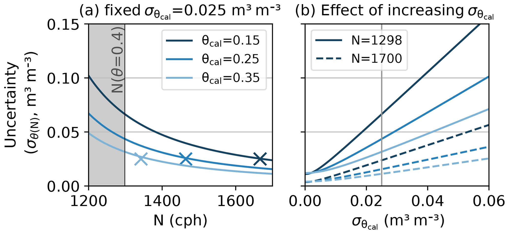
Figure 2 Standard deviation of θ^L(N) in the case where a local value of N₀ is estimated from a local reference measurement of SWC (see scenario 1 in Table 2). Panel (a) shows the dependence of the error on the wetness conditions during calibration (i.e. θ_cal) assuming an arbitrarily fixed error in ${\mathit{\sigma }}_{{\mathit{\theta }}_{\mathrm{cal}}=\mathrm{0.025}}$ m³ m⁻¹. The “x” markers highlight the neutron intensity during calibration (N_cal) for the SWC corresponding to θ_cal. Panel (b) shows the error for increasing values of ${\mathit{\sigma }}_{{\mathit{\theta }}_{\mathrm{cal}}}$ at two neutron intensity levels (dashed lines for dry conditions, solid lines for wet conditions); colours are explained by the legend in panel (a). The vertical grey line corresponds to the value of ${\mathit{\sigma }}_{{\mathit{\theta }}_{\mathrm{cal}}}$, which was fixed for panel (a).

While we have to make assumptions about the standard deviation (or error) of most involved parameters, the uncertainty σ_N of the neutron count rate N (in cph) is a result of the stochastic nature of the counting process and amounts to $\sqrt{N}/\sqrt{\mathrm{\Delta }t}$ for an integration period of Δt (in hours; in this study, we always use Δt=24 h). As a result, the relative uncertainty in N increases with decreasing N (and hence increasing θ). This fact is well known (see, e.g. Francke et al., 2022) and clearly visible in Fig. 2a. The same figure, however, shows that the increase in σ_θ(N) with decreasing N very much depends on the wetness conditions under which the calibration was carried out: for the same value of N, the error in θ(N) is higher in the case the calibration was carried out under drier conditions. While this behaviour is plausible, it might appear surprising at first and, to our knowledge, has not been previously described. The same error in θ_cal will be amplified under wet conditions when the calibration was carried out under dry conditions, whereas the error will be attenuated under dry conditions if the calibration was carried out under wet conditions. This is only partly due to the fact that the same value of ${\mathit{\sigma }}_{{\mathit{\theta }}_{\mathrm{cal}}}$ implies different relative errors under wet and dry conditions. The more important effect is the different slope of the Desilets function under wet and dry conditions.

Figure 2b shows the effect of increasing values of ${\mathit{\sigma }}_{{\mathit{\theta }}_{\mathrm{cal}}}$, again for the three different calibration conditions. For each of the three θ_cal, we show the error for two values of N – one for wet (solid line) and one for dry conditions (dashed line). The solid dark blue line gives us a kind of worst case scenario, with σ_θ exceeding values of 0.15 m³ m⁻³. However, we should keep in mind that SWC will typically vary between wilting point and field capacity (or porosity at the maximum), which spans a limited dynamic range of SWC for most soils.

Before turning to the general calibration function, we should note that the error in soil bulk density (${\mathit{\sigma }}_{{\mathit{\rho }}_{\mathrm{b}}}$) does not propagate to θ^L(N) (not shown in the figure). The reason is that the influence of bulk density basically cancels out as it appears in the enumerator and denominator of Eq. (10). This is different for the general calibration function, the results of which are shown in Fig. 3.

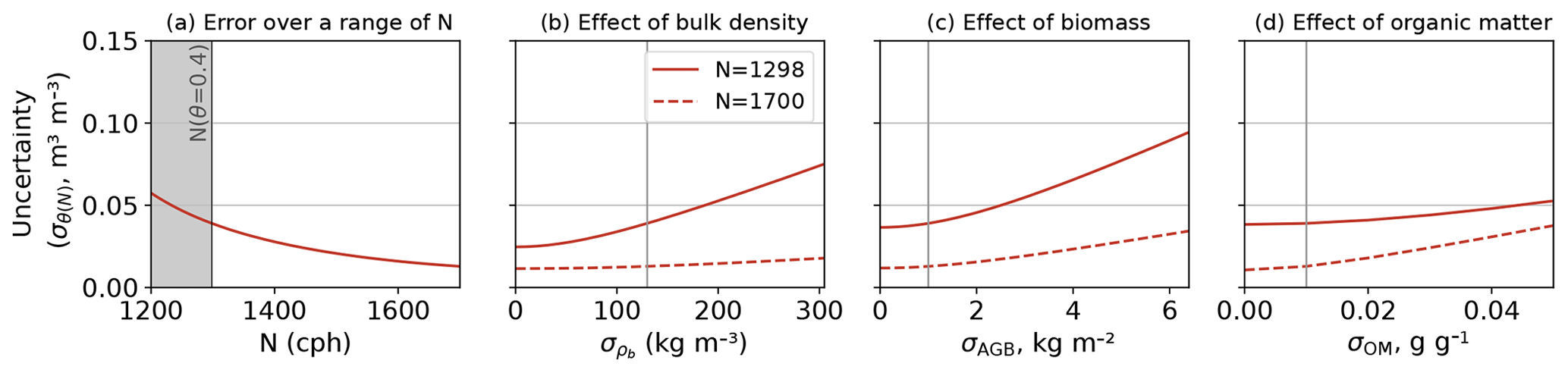
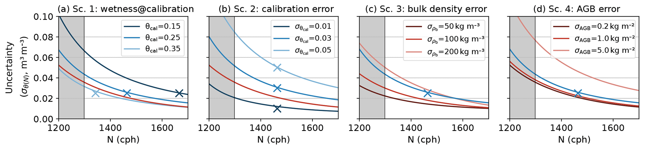
Figure 3 Standard deviation of θ(N) in the case of a general calibration. Panel (a) shows the error in θ^G(N) for parameters shown in Table 2, scenario 1. (b–d) Same parameters, except for the errors in bulk density (b), above-ground biomass (c), and organic matter content (d). The vertical grey lines mark the values of the corresponding error that were used to create panel (a).

The layout of Fig. 3 is similar to Fig. 2. As the general calibration strategy relies on a single location-independent value of N₀, no different calibration conditions need to be compared here. However, more parameters can potentially propagate their errors. Figure 3a shows the error for a parameter combination that is referred to as scenario 1 in Table 2. The resulting curve is similar to the light blue curve in Fig. 2a (high wetness during calibration). Figure 3b–d illustrates how the error in θ^G(N) changes with the errors in bulk density, above-ground biomass, and soil organic matter content. Specifically under wet conditions (N=1298 cph, corresponding to θ=0.4 m³ m⁻³), large errors in the estimation of soil bulk density or biomass in the sensor footprint will substantially increase the error in θ^G(N), which is to be expected. For biomass, though, it must be emphasized that the upper range of errors in the estimation of biomass are only expected to occur in forested areas (where, at least for temperate conditions, total above-ground dry biomass typically ranges between 10 and 40 kg m⁻²). In grassland or cropland, however, above-ground dry biomass will mostly not exceed 1 kg m⁻², so that the corresponding estimation error is expected to remain much lower.

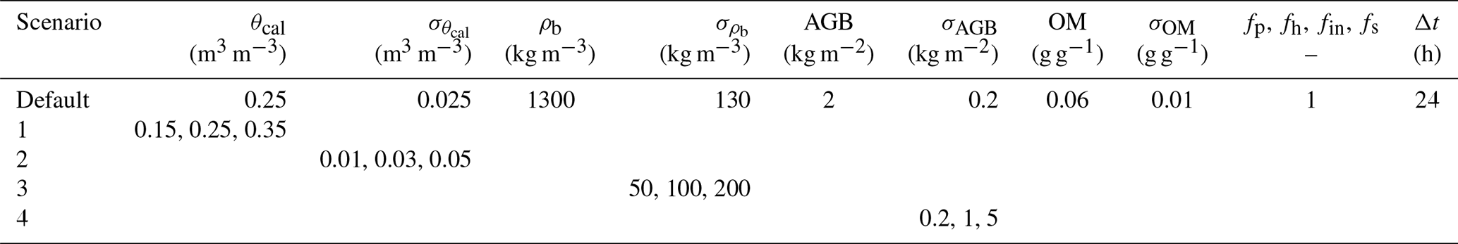
Table 2 Parameter combinations for the scenarios evaluated in this study. Note that neither the general calibration (Eq. 2) nor the local one (Eq. 10) uses all parameters contained in one row of the table (e.g. θ_cal is only used for local, not general calibration).

We would like to come back to our question of which strategy, local or general, is recommended in terms of minimizing the error in θ(N). The above results suggest that there is no general answer to that question. Instead, the answer depends on the specific combination of parameters and errors that we expect to govern the sensor's response and the data sampled within its footprint. Unfortunately, we usually do not know these values, particularly in the case of soil or biomass sampling where we are dealing with limited sample sizes or, even worse, a lack of representativeness. But while we might not know the exact errors we are dealing with, we might at least be able to make an educated guess, to narrow down the ranges, or give maximum error estimates. For instance, as mentioned above, we can be very certain that the error in our above-ground biomass estimate will not exceed 1 kg m⁻² in a grassland or cropland location. Based on the relationships shown in Fig. 3, CRNS users might also decide to increase their sampling efforts (for any variable such as θ_cal, ρ_b, or AGB) until they can be confident that the error in that variable remains within a desired range.

Figure 4 directly compares the two calibration strategies for a few selected scenarios (Table 2) in order to convey some basic guidance. As shown above, for the local calibration, θ(N) degrades substantially with increasing errors in θ_cal (scenario 2). For the general calibration, the uncertainty in θ(N) is governed by the errors in bulk density and biomass (see scenarios 3 and 4). While this qualitative behaviour is unsurprising, the strength of such a visualization is that it quantitatively contrasts the results for potential application contexts. Thus, it becomes obvious that the general calibration outperforms the local one for agricultural landscapes (low biomass error) and moderate errors in bulk density and θ_cal, while the local calibration is clearly preferable in forest environments, unless very reliable biomass estimates are available.

Figure 4 Similar to Figs. 2a and 3a but for four different scenarios (“Sc.”; see Table 2 for the definition of the scenarios). Blueish colours correspond to the local, reddish colours to the general calibration strategy.

For users who would like to explore how the two calibration strategies compare in their specific application context, we provided an interactive online tool: https://cosmic-sense.github.io/local-or-global (last access: 23 February 2024).

5 Conclusions

We tested a general functional relationship θ^G(N) to estimate SWC from observed neutron intensities, without the need for a local calibration. θ^G(N) is based on the widely used Desilets function, and takes into account various variables which govern the neutron intensity observed in a specific location. To calibrate and test θ^G(N), we used four recently published datasets with a total of 75 CRNS locations and 104 calibration dates. This constitutes the most comprehensive analysis of CRNS calibration conducted to far.

Apart from accounting for the local effects of vegetation, soil organic matter, lattice water, and bulk density, two features were essential to achieve the desired level of generalization, i.e. to estimate one single value of N₀ across all CRNS locations.

• Accounting for detector efficiency was possible thanks to comprehensive instrumental efforts undertaken during campaigns in the context of the three dense CRNS clusters. In these campaigns, CRNS sensors were systematically collocated with a so-called “calibrator” probe so that we were able to determine either specific sensitivity factors for individual neutron detectors or average sensitivity factors for the most common types of detectors, relative to that “calibrator” probe. Evidently, we cannot apply θ^G(N) if the relative sensitivity of the neutron detector is unknown. This is a fundamental caveat, although prospective research might find ways to address this issue, e.g. by considering neutron detectors as nodes in a topological network so they could be cross-calibrated across multiple edges of such a network or by simulating response functions of CRNS detector designs (see, e.g. Köhli et al., 2018).

• We used the PARMA model (Sato, 2015) in order to account for the spatial variability in incoming neutron intensity (relative to a reference location), as a function of geographic latitude and longitude as well as terrain altitude. While the PARMA model is well established, its application in this study remains as an example and a subjective choice. Other similar models exist (e.g. Desilets and Zreda, 2003; Hawdon et al., 2014; McJannet and Desilets, 2023), and future research should aim to explore the potential sensitivity of the neutron intensity scaling to the choice of the model and the consistency of the resulting soil moisture estimates.

Altogether, we assume that we have considered the most relevant processes and variables (except for the presence of snow and for topographic shielding). On average, the general calibration function fits the weighted average of locally measured SWC per CRNS footprint fairly well, specifically for the apparent gravimetric SWC. Looking at volumetric soil moisture, though, the mean absolute error between θ^G(N) and the calibration reference θ_cal amounts to 0.075 m³m⁻³, which is quite substantial.

If we trust the general structure of our function θ^G(N), this error can have two basic sources: the uncertainty in θ_cal and the uncertainty in the parameters in θ^G(N). We expect both parts to be error prone, and cannot quantify either one with confidence. Interestingly, though, we only become aware of these errors in the case where we apply a general calibration. If we calibrate N₀ locally, we will, by definition, force θ^L(N_cal) and θ_cal to be equal at the date of calibration.

Most CRNS users only consider opting out of local N₀ calibration if local reference measurements of SWC are impossible, e.g. due to stony soils or restricted access, or in the case of CRNS roving. Based on the results of this study, we recommend considering both calibration options, local and general, and weighing their relative uncertainties against one another. We used Gaussian error propagation for that purpose. Unsurprisingly, the error in θ^L(N) is governed by the error in the calibration reference θ_cal. However, it was interesting for us to note how the propagation of this error depends on the value of θ_cal itself: if the calibration were carried out under dry conditions, the error would grow substantially under wet application conditions. Considering further that the spatial variability in soil moisture appears to reach a maximum under intermediate wetness conditions (see, e.g. Famiglietti et al., 2008; Crow et al., 2012), it might be recommendable to obtain θ_cal under rather wet conditions. Please note, however, that we only analysed the error in the local calibration scenario in the case of a single calibration date (while it is recommended to carry out multiple calibration campaigns, this is not yet common practice). The overall error in θ^L(N) is expected to decrease for multiple calibration dates, and future studies should aim to explicitly represent the corresponding error propagation.

The error in θ^G(N), in turn, is governed by the errors in vegetation biomass and bulk density. Altogether, there is no general answer as to which calibration option is preferable. Based on our results, though, users should be aware that even in the presence of local calibration measurements, actually applying a local calibration might not necessarily be the best option. Instead, we provide an interactive tool so that users can weigh the options in their specific application context or decide how much additional sampling efforts are required to reduce the uncertainty in either calibration option.

We would like to emphasize that our formulation of a general calibration function should be considered a mere suggestion. Other functions might be better suited, either for the overall relationship between θ and N (such as the one provided by Köhli et al., 2020, specifically under dry conditions) or for the individual components that are required to scale the observed neutron intensities (e.g. to account for vegetation biomass or the spatial variability in the incoming neutron flux). The resulting value of N₀ will depend much on the specific scaling techniques, so our value of 2306 cph should not be over-interpreted. Rather than providing a universal calibration function with a universal N₀, the key lesson of this study is that it is worth using a multiplicity of locations to calibrate any θ(N) relationship, even if you are interested in only one specific location yourself. The CRNS datasets for such analyses are openly available to everyone, so other ideas can be explored.