A comprehensive study of deep learning for soil moisture prediction

Soil moisture plays a crucial role in the hydrological cycle, but accurately predicting soil moisture presents challenges due to the nonlinearity of soil water transport and the variability of boundary conditions. Deep learning has emerged as a promising approach for simulating soil moisture dynamics. In this study, we explore 10 different network structures to uncover their data utilization mechanisms and to maximize the potential of deep learning for soil moisture prediction, including three basic feature extractors and seven diverse hybrid structures, six of which are applied to soil moisture prediction for the first time. We compare the predictive abilities and computational costs of the models across different soil textures and depths systematically. Furthermore, we exploit the interpretability of the models to gain insights into their workings and attempt to advance our understanding of deep learning in soil moisture dynamics. For soil moisture forecasting, our results demonstrate that the temporal modeling capability of long short-term memory (LSTM) is well suited. Furthermore, the improved accuracy achieved by feature attention LSTM (FA-LSTM) and the generative-adversarial-network-based LSTM (GAN-LSTM), along with the Shapley (SHAP) additive explanations analysis, help us discover the effectiveness of attention mechanisms and the benefits of adversarial training in feature extraction. These findings provide effective network design principles. The Shapley values also reveal varying data leveraging approaches among different models. The t-distributed stochastic neighbor embedding (t-SNE) visualization illustrates differences in encoded features across models. In summary, our comprehensive study provides insights into soil moisture prediction and highlights the importance of the appropriate model design for specific soil moisture prediction tasks. We also hope this work serves as a reference for deep learning studies in other hydrology problems. The codes of 3 machine learning and 10 deep learning models are open source.

1 Introduction

Soil moisture is significant with respect to simulating many hydrological processes, as it controls the interaction of water and energy between the land surface and the atmosphere (Entin et al., 2000; Vereecken et al., 2022). Accurately providing information on soil moisture dynamics is crucial for effective water resources planning and management, agricultural production, climate prediction, and flood disaster monitoring (Vereecken et al., 2008; Sampathkumar et al., 2013). However, due to the randomness of rainfall and the nonlinear features of infiltration and evaporation processes (Guswa et al., 2002), soil moisture is highly variable and nonlinear in space and time (Heathman et al., 2012), making it difficult to forecast.

As various mainstream approaches have been applied to soil moisture dynamics prediction, a comprehensive study is needed to provide suitable solutions for different predicting tasks, encourage improvements on models, and build confidence in this area. Traditionally, soil moisture dynamics prediction is widely based on physical models, such as the soil–plant–air model (Saxton et al., 1974), HYDRUS (Simunek et al., 2005), and CATHY (Camporese et al., 2015). Although these models are interpretable, they perform poorly in practical applications, because of the inestimable parameters (Gill et al., 2006) and inadequate description of physical processes (Li et al., 2022b). With the reduction in data acquisition costs and advancements in computation, there has been an increasing focus on data-driven models. Initially, multiple linear regression (Qiu et al., 2003; Hummel et al., 2001) and empirical models (Azhar et al., 2011; Verma and Nema, 2021) are applied to soil moisture prediction. However, one non-negligible problem is that these methods require calibrations and have limited generalization capabilities (Holzman et al., 2017; Jackson, 2003). Compared with these traditional data-driven models, machine learning methods appear to possess a stronger data fitting ability. For instance, support vector regression (SVR) (Gill et al., 2006) and random forest (RF) (Prasad et al., 2019) have both shown satisfactory and robust results with low computing costs in soil moisture prediction. Additionally, the single-layer feedforward neural network with generalized inverse operation – extreme learning machine (ELM) (Huang et al., 2006) – can precisely predict the future trends of soil moisture and support future irrigation scheduling (Liu et al., 2014). Moreover, when dealing with multi-scale soil moisture data, such as satellite data, Abbaszadeh et al. (2019) employed 12 distinct random forest models to downscale the daily composite version of Soil Moisture Active/Passive (SMAP) data.

Currently, deep learning is the state-of-the-art data-driven method and has made obvious improvements in many research areas (Lecun et al., 2015). Due to their powerful approximation ability, deep neural networks (DNNs) (Goodfellow et al., 2016) have been extensively applied in soil moisture descriptions (Cai et al., 2019; Prakash et al., 2018). Notably, recurrent neural networks (RNNs) (Pollack, 1990) excel at capturing temporal information in time series' data and model sequential dependencies for predictions (Mikolov et al., 2011). This is consistent with the characteristics of soil moisture dynamics simulation. Fang et al. (2019) utilized long short-term memory (LSTM) (Hochreiter and Schmidhuber, 1997) for soil moisture and received satisfactory results. Furthermore, Sungmin et al. (2021, 2022) efficiently employed LSTM to interpolate global gridded datasets from in situ observations (Sungmin and Orth, 2021; Sungmin et al., 2022). From a different perspective, convolution neural networks (CNNs) (LeCun, 1989) are capable of extracting features from training data in specific dimensions, making them widely used in dealing with two-dimensional (Albawi et al., 2018; Patil and Rane, 2021) or one-dimensional data (Severyn and Moschitti, 2015; Shi et al., 2015). Therefore, 1D-CNNs are applied in many hydrology research endeavors (Hussain et al., 2020; Chen et al., 2021). Additionally, attention mechanisms enable the selection of critical information from multiple input features or model outputs, which can be visualized using attention weight (Ding et al., 2020; Li et al., 2022a). On this foundation, self-attention can model dependencies and aggregate features from inputs while disregarding their distance (Vaswani et al., 2017), which shows great potential in soil moisture prediction.

As various deep learning approaches have focused on distinct data utilization mechanisms, hybrid structures have become a vital research area. On one hand, combining the feature importance processing methods – attention mechanisms – with deep learning models, can indeed lead to improvements (Ahmed et al., 2021; Ding et al., 2019; Kilinc and Yurtsever, 2022). Li et al. (2022) proposed an attention-aware LSTM to estimate soil moisture and temperature and achieved better performance than LSTM alone. In their work, three attention mechanisms help obtain the spatial–temporal feature vectors of LSTM inputs or outputs. On the other hand, the combinations of multiple neural networks tend to perform better than a single network alone (Semwal et al., 2021). The hybrid CNN–GRU model proposed by Yu et al. (2021) outperformed the independent CNN or GRU model in predicting root zone moisture. Moreover, Li et al. (2022b) proposed EDT-LSTM, a stacked LSTM model based on the encoder–decoder structure (Sutskever et al., 2014) and residual learning (He et al., 2016). This achieved more stable results than a single LSTM. Regarding the optimization of training strategies, adversarial training in generative adversarial networks (GANs) (Goodfellow et al., 2014) can capture more information on real data. This helps to address the problem of fuzzy prediction and provides a superior solution for weather forecasts (Jing et al., 2019; Ravuri et al., 2021). Moreover, advancements in model structure have been instrumental in enhancing performance and improving generalization abilities. For instance, Liu et al. (2022) integrated multi-scale designs into their models. In addition to pure deep learning models, differentiable, physics-informed machine learning models with a physical foundation have emerged as a noteworthy development. This kind of model systematically integrates physical equations with deep learning, enabling the prediction of untrained variables and processes with high accuracy (Feng et al., 2023).

Therefore, it is essential to design effective and suitable neural network structures for soil moisture prediction tasks. In this study, we comprehensively evaluate the performance of various deep learning methods in soil moisture prediction, highlighting their key characteristics in terms of prediction accuracy and computational costs. The models evaluated in this research range from machine learning models, such as RF, ELM, and SVR, to basic deep learning models, including 1D-CNN, LSTM, and the encoder of Transformer (Vaswani et al., 2017), and hybrid deep learning models, including CNN–LSTM, LSTM–CNN, CNN-with-LSTM, feature attention LSTM (FA-LSTM), temporal attention LSTM (TA-LSTM), feature and temporal attention LSTM (FTA-LSTM), and generative-adversarial-network-based LSTM (GAN-LSTM). Notably, the encoder of the Transformer is first developed in soil moisture prediction, with CNN–LSTM, LSTM–CNN, FA-LSTM, TA-LSTM, FTA-LSTM, and GAN-LSTM first applied and systematically compared for soil moisture. To gain insights into their workings and provide a thorough analysis of why some methods perform better, we utilize the Shapley (SHAP) (Lundberg et al., 2018) method to demonstrate the importance of features in different models and employ t-distributed stochastic neighbor embedding (t-SNE) visualization (Van der Maaten and Hinton, 2008) to show the encoded features across models. The systematical assessment of the models is carried out across multiple sites at five depths. For forecasting soil moisture, the utilized data include meteorological data, soil temperature data, and soil moisture content data from previous days, as these inputs are closely associated with evaporation and infiltration processes.

In the remainder of this article is structured as follows: Sect. 2 describes the data used and the deep learning background; Sect. 3 presents a detailed description of the participating methods; Sect. 4 analyzes comparison results and discusses the interpretability of the models; and the conclusion is drawn in Sect. 5.

2 Data description and background

2.1 Data description

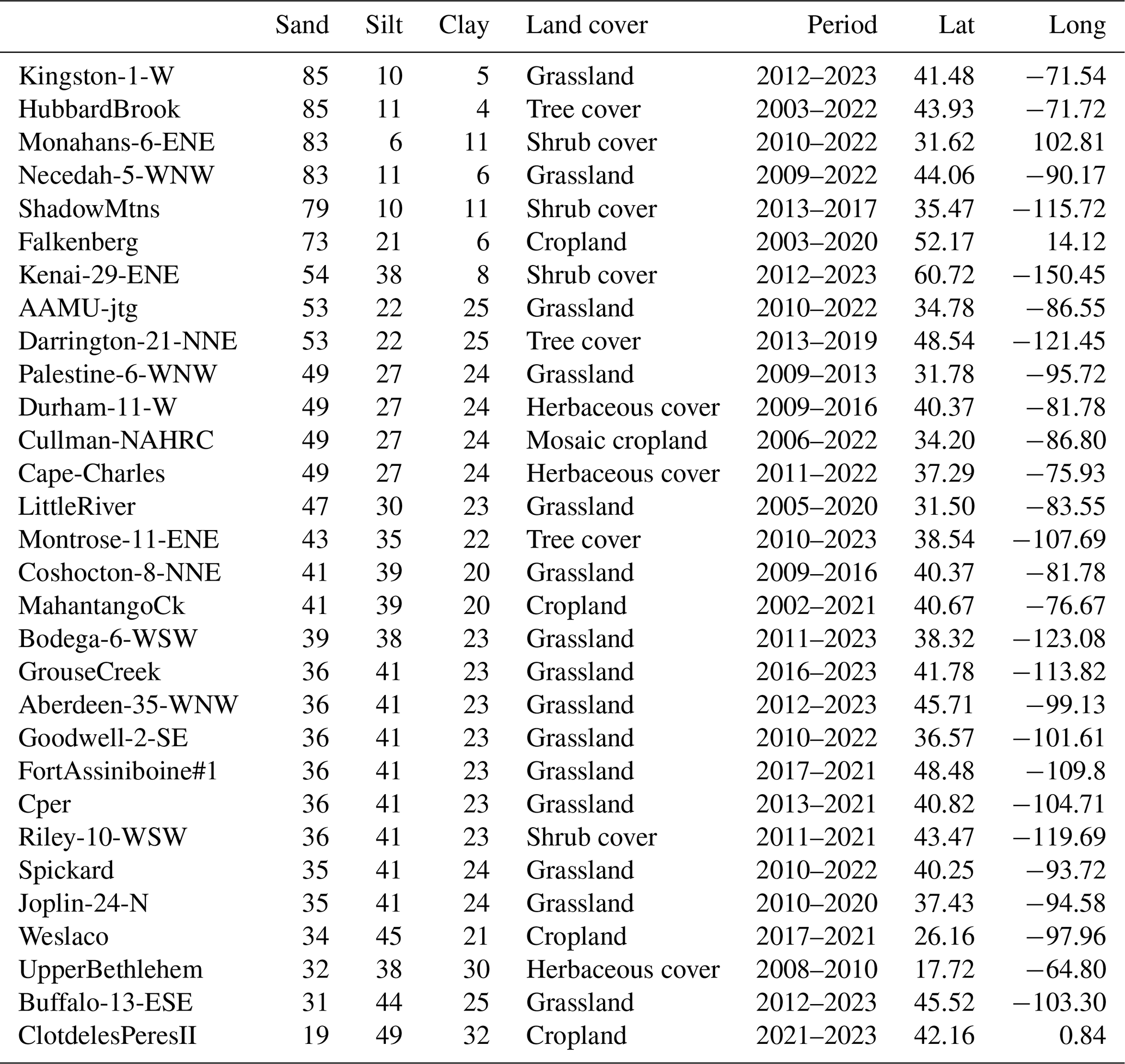
To create a comprehensive evaluation under different soil types, in situ observations at 30 different sites are downloaded from the International Soil Moisture Network (ISMN) (https://ismn.earth/en/dataviewer/, last access: 20 February 2024). The research sites are carefully chosen according to the geographical location (as dispersed as possible), soil textures, and distinct land cover types (as diverse as possible). The main characteristics of the selected sites are shown in Table 1. The spatial locations of the sites are shown on a world map in Fig. 1. More detailed site meteorological information and soil moisture time series' data are provided in Appendix D.

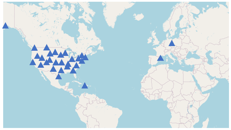
Figure 1 The spatial locations of the 30 selected sites.

During the input factor screening process, we carefully choose meteorological inputs based on the precipitation and evapotranspiration calculation, including precipitation (P), atmospheric temperature (AT), longwave radiation (LR), shortwave radiation (SR), wind speed (WS), and relative humidity (RH), which are closely related to the soil evapotranspiration and infiltration processes. Moreover, soil temperature (ST) data and soil moisture (SM) data from the previous day are incorporated to represent the soil condition. Figure 2 displays the Pearson correlation analysis results for input factors at the Cape-Charles and UpperBethlehem sites. Pearson correlation analysis examines the relationship between two variables by calculating the correlation coefficient, thereby measuring the strength and direction of their association. Notably, the correlation coefficients between soil moisture and the input data vary greatly with respect to both the station and depth. While the correlation coefficient between longwave radiation and soil moisture is low at the UpperBethlehem site, it is significant at the Cape-Charles site, highlighting the influence of site-specific differences. Although utilizing highly correlated factors as inputs appears to be a logical choice, achieving uniformity across different sites and depths can be difficult. This presents a crucial aspect to explore when evaluating the performance of models for self-learning screening of significant influencing factors. Therefore, the input data x_t at time t consist of all eight factors, ${\mathit{x}}_t=\left\{P_t,T_t,{\mathrm{LW}}_t,{\mathrm{SW}}_t,{\mathrm{RH}}_t,{\mathrm{WS}}_t,{\mathrm{ST}}_t,{\mathrm{SM}}_{t-\mathrm{1}}\right\}$. As groundwater level observations are difficult to obtain, changes in the lower boundary conditions are excluded from the inputs.

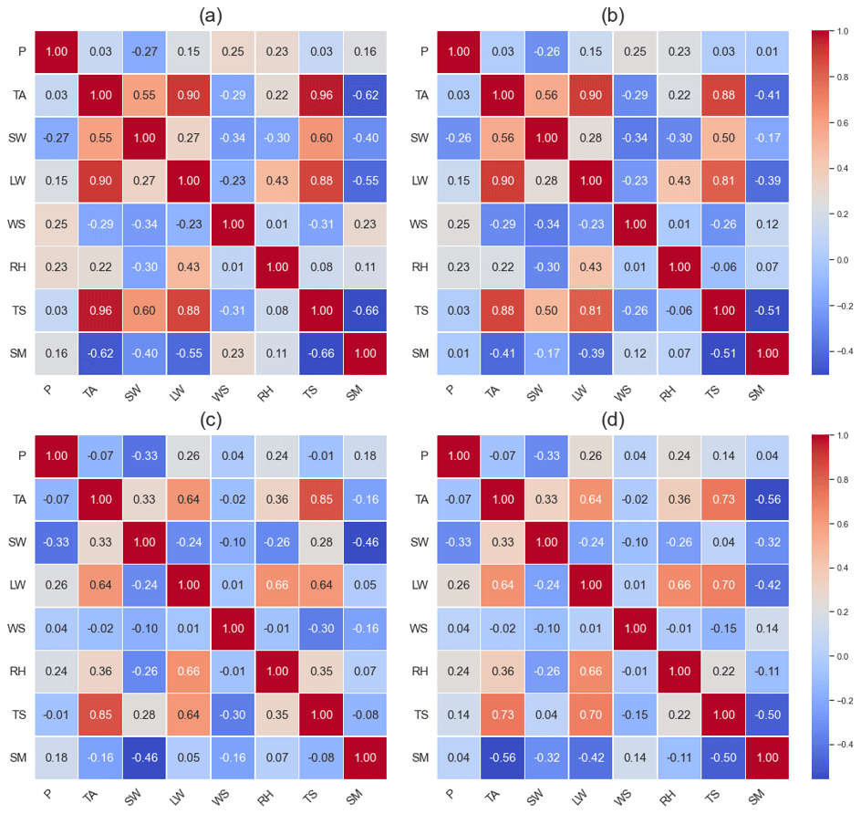
Figure 2 Pearson correlation analysis results among the observed variables at 0.05 and 1.00 m at the Cape-Charles (a–b) and UpperBethlehem (c–d) sites.

Figure 3 shows the autocorrelation analysis conducted at five soil depths. The autocorrelation coefficients for soil water content at different depths decrease with an increasing number of delay days. The most significant change is observed in the surface layer. As a result, we have utilized a 4 d delay as our input for all deep learning models in this study to forecast the soil moisture content on the fifth day. This means the input vector $\mathit{I}\left\{{\mathit{x}}_{t-\mathrm{3}},{\mathit{x}}_{t-\mathrm{2}},{\mathit{x}}_{t-\mathrm{1}},{\mathit{x}}_t\right\}$ is used to predict the target value y_t, which is the soil moisture SM_t at time t. For machine learning, we only utilize the x_t to generate predictions.

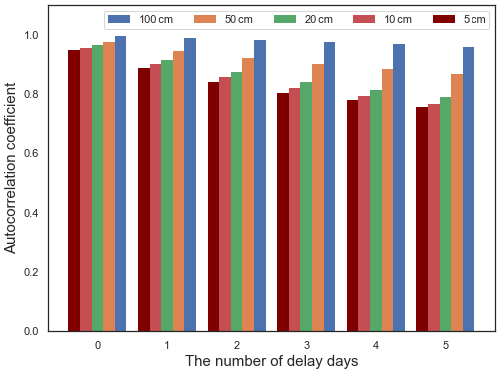
Figure 3 Autocorrelation analysis results of soil water content with different numbers of delay days at the Cape-Charles site.

This study builds individual predictive models for each site and depth, disregarding the inclusion of static properties such as land cover, soil hydraulic properties, and topography. Soil moisture and soil temperature data are obtained from the ISMN. Specifically, the meteorological data applied in this work are sourced from the NASA Prediction Of Worldwide Energy Resources (POWER) project (https://power.larc.nasa.gov/, last access: 20 February 2024), which provides a wide range of meteorological data, such as temperature, precipitation, and solar radiation. Detailed information can be found at (https://power.larc.nasa.gov/docs/methodology/data/sources/, last access: 20 February 2024). The meteorological data are used as an auxiliary component for soil moisture prediction in our work. Therefore, even though the resolution of some variables appears coarse, we can safely disregard the potential influence of resolution on our research findings and conclusions.

Table 1 Summary of main characteristics of the 30 sites.

2.2 Deep learning backgrounds

Deep learning enhances the complexity and learning capability of traditional machine learning methods by adding multiple layers (Kamilaris and Prenafeta-Boldú, 2018). At each layer, input signals are weighted through the connections of each neuron and are subsequently activated by activation functions (Schmidhuber, 2015). Deep learning discovers intricate structures in training data by utilizing backpropagation to guide the machine with respect to adjusting its internal parameters (Lecun et al., 2015).

In this study, the primary challenge in soil moisture prediction is processing the time series' data with specific dimensions and simulating soil moisture dynamics with high spatiotemporal variability. Given the diversity of neural networks, numerous methods have the potential to deal with specific time series' data. CNNs can extract local temporal information from the data by sliding convolutional kernels along the time dimension. On the other hand, RNNs excel at capturing the overall temporal sequence information. Additionally, self-attention has the potential to associate inputs and make predictions, making them capable of handling sequential data effectively. These three types of networks can be regarded as fundamental feature extractors in deep learning. Furthermore, hybrid deep learning models integrate the characteristics of multiple models, enhancing their prediction capacities (Yu et al., 2021). Combinations of CNNs, RNNs, and attention mechanisms have been widely utilized in many studies. Furthermore, employing specified training strategies with suitable network structures can also improve prediction performance. For instance, GANs enable the training objective of neural networks to go beyond minimizing data mean-square error and to utilize adversarial training to fully capture data regularities. By designing appropriate network structures and training strategies, it is possible to further improve prediction accuracy.

It is necessary to conduct a comprehensive evaluation to analyze the internal mechanisms of models and decide on the most suitable combination rule for soil moisture prediction. With the collected data in Sect. 2.1, it is possible to deeply explore the prediction abilities of the deep learning models. We evaluate models from the perspectives of prediction accuracy and computational costs to provide a reference for soil moisture dynamics predictions. Further research on model interpretability can provide insights into how the model structure influences the utilization of data, leading to a more effective model structure design.

3 Models and methodology

Three machine learning models and seven deep learning models take part in this comparative research. Introductions to each model are provided below, along with key references for interested readers. The parameters of each model are recorded in Appendix A.

3.1 Machine learning methods

In this study, random forest (RF), extreme learning machine (ELM), and support vector machine (SVM) machine learning models are applied to compare with the deep learning models as a benchmark.

Random forest, proposed by Breiman (2001), is used for regression and classification tasks and has gained popularity for its high accuracy. RF works by constructing multiple decision trees on randomly sampled subsets of the training data. Each tree is trained on a random subset of features, and the final prediction is made by averaging the predictions of the individual trees. This approach reduces overfitting and increases model stability. For soil moisture prediction, RF has proven to be a stable and reliable method (Carranza et al., 2021).

Extreme learning machine (Huang et al., 2006) utilizes a single-layer feedforward neural network as its foundation. ELM achieves a fast learning speed and strong generalization ability by employing random input layer weights and biases and applying generalized inverse matrix theory to calculate the output layer weights. The algorithm has been applied in various fields and has shown promising results. Liu et al. (2014) employed ELM to predict the large-scale soil moisture in Australian orchards. The results demonstrated that the model was capable of accurate forecasting.

Support vector machine (Cortes and Vapnik, 1995) was proposed for applications in classification and regression. It aims to find the maximum-margin hyperplane that best separates sample points. To make this hyperplane more robust in high-dimensional feature spaces, SVM uses kernel functions to perform nonlinear mapping and create a new feature space where the data can be linearly separable. The algorithm then finds the optimal classification hyperplane with the maximum margin. SVMs have achieved great success in various fields. Gill et al. (2006) applied SVM to soil moisture prediction and compared it with DNNs. The results showed that SVM was suitable for soil moisture content prediction. Support vector regression (SVR), which is applied in this study, is a variant of SVM that is specifically designed for regression tasks.

For machine learning, x_t and y_t represents the input feature and target object, respectively. The input data correspond one-to-one in time to the target and serve as both the input and output of the machine learning models. The prediction accuracy of machine learning serves as a comparison for deep learning models. Hyperparameters used in models are recorded in Appendix A.

3.2 Basic deep neural networks

3.2.1 LSTM

RNNs (Pollack, 1990) operate by recursing in the direction of sequence progression, with all nodes in the network being chained together. These unique properties make RNNs effective with respect to processing sequential data and extracting temporal information, which has led to breakthroughs in natural language processing (Connor et al., 1994). The ability of RNNs to model temporal dependencies is suitable for predicting soil moisture.

LSTM (Hochreiter and Schmidhuber, 1997) neural networks were proposed to address the limitations of traditional RNNs. LSTM can overcome the issue of gradient vanishing and memorize more useful information through a special unit, which is called the cell state. Thus, LSTM operates as follows:

$$\begin{array}{}\text{(1)}& {\displaystyle }{\mathit{i}}_t=\mathit{\sigma }\left({\mathbf{W}}_{\mathrm{i}}\cdot \left[{\mathit{h}}_{t-\mathrm{1}},{\mathit{x}}_t\right]+{\mathit{b}}_{\mathrm{i}}\right),\text{(2)}& {\displaystyle }{f}_t=\mathit{\sigma }\left({\mathbf{W}}_{\mathrm{f}}\cdot \left[{\mathit{h}}_{t-\mathrm{1}},{\mathit{x}}_t\right]+{\mathit{b}}_{\mathrm{f}}\right),\text{(3)}& {\displaystyle }{\mathit{o}}_t=\mathit{\sigma }\left({\mathbf{W}}_{\mathrm{o}}\cdot \left[{\mathit{h}}_{t-\mathrm{1}},{\mathit{x}}_t\right]+{\mathit{b}}_{\mathrm{o}}\right),\text{(4)}& {\displaystyle }{\stackrel{\mathrm{̃}}{\mathit{C}}}_t=\tan h\left({\mathbf{W}}_{\mathrm{c}}\cdot \left[{\mathit{h}}_{t-\mathrm{1}},{\mathit{x}}_t\right]+{\mathit{b}}_{\mathrm{c}}\right),\text{(5)}& {\displaystyle }{\mathit{c}}_t=f_t\cdot {\mathit{c}}_{t-\mathrm{1}}+i_t\cdot {\stackrel{\mathrm{̃}}{\mathit{C}}}_t,\text{(6)}& {\displaystyle }{\mathit{h}}_t={\mathit{o}}_t\cdot \tan h\left({\mathit{c}}_t\right).\end{array}$$

Here, W_i and b_i are the parameters for the input gate, W_f and b_f are the parameters for the forget gate, W_o and b_o are the parameters for the output gate, W_c and b_c are used for cell state updating, and σ is the activation function.

We generate the time-dependent hidden states $\mathit{H},\left\{{\mathit{h}}_{t-\mathrm{3}},{\mathit{h}}_{t-\mathrm{2}},{\mathit{h}}_{t-\mathrm{1}},{\mathit{h}}_t\right\}$ from input $\mathit{I},\left\{{\mathit{x}}_{t-\mathrm{3}},{\mathit{x}}_{t-\mathrm{2}},{\mathit{x}}_{t-\mathrm{1}},{\mathit{x}}_t\right\}$ through the LSTM. After sequentially processing all inputs in the LSTM, the last hidden state h_t of the sequential output is used as the prediction for network training, as depicted in Fig. 4a. This is because the input features at each time step can be encoded in the last hidden state. The parameters in this model are recorded in Appendix A.

3.2.2 1D-CNN

CNNs (LeCun, 1989) were originally applied to image recognition. The convolution and pooling layers in CNNs can extract the distinguishing features of the given data while reducing the number of data to be processed (Ajit et al., 2020). Consequently, CNNs are highly effective in processing data that come in the form of multiple arrays.

For time series' data, 1D-CNNs can extract local temporal features via convolution kernels that slide along the time dimension. The 1D-CNNs have demonstrated success in speech and natural language processing applications (Abdel-Hamid et al., 2014; Severyn and Moschitti, 2015). Hence, 1D-CNNs are capable of soil moisture prediction tasks. The complete forward-propagation process of a simple 1D-CNN for soil moisture prediction is illustrated in Fig. 4b. Given that the input vector $\mathit{I},\left\{{\mathit{x}}_{t-\mathrm{3}},{\mathit{x}}_{t-\mathrm{2}},{\mathit{x}}_{t-\mathrm{1}},{\mathit{x}}_t\right\}$, two convolution layers are employed in the 1D-CNN architecture. The convolution kernel size (Kernel_size) is set to 2, with a stride of 1. Specific parameters are listed in Table A1. To preserve the information in the data, pooling layers are intentionally omitted.

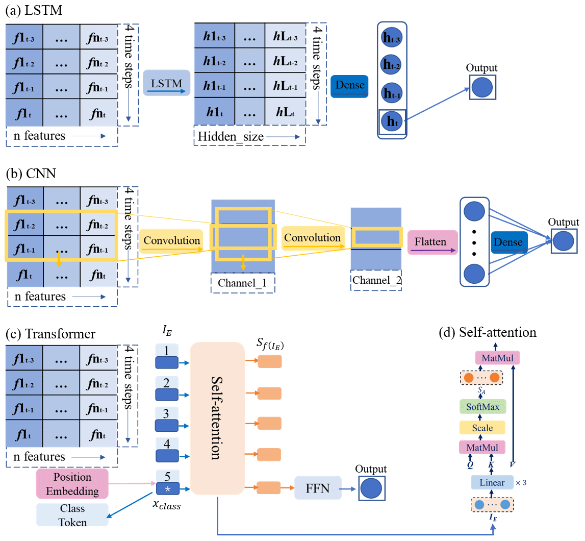
Figure 4 Network structures of the LSTM (a), the 1D-CNN (b), and the proposed Transformer (c), inspired by Dosovitskiy et al. (2020), with the self-attention structure (d) for soil moisture prediction.

3.2.3 Transformer

The self-attention mechanism can model the dependencies and aggregate features from inputs. Therefore, a stacking structure of self-attention mechanisms like Transformer (Vaswani et al., 2017) can achieve the functions of CNNs and RNNs without iterations. This provides a novel way for predictions to be made. In this study, we utilize the encoder structure of the Transformer (Vaswani et al., 2017), as depicted in Fig. 4c, to predict soil moisture. The self-attention is shown in Fig. 4d and operates as follows:

$$\begin{array}{}\text{(7)}& {\displaystyle }{S}_A=\mathrm{softmax}\left({\displaystyle \frac{{\mathbf{QK}}^T}{\sqrt{d_k}}}\right)=\mathrm{softmax}\left({\displaystyle \frac{\left({\mathbf{W}}_{\mathrm{Q}}{I}_E\right){\left({\mathbf{W}}_{\mathrm{K}}{I}_E\right)}^T}{\sqrt{d_k}}}\right),\text{(8)}& {\displaystyle }{S}_{\mathrm{f}}\left(I_E\right)=S_A\otimes V=\mathrm{softmax}\left({\displaystyle \frac{\left({\mathbf{W}}_{\mathrm{Q}}{I}_E\right){\left({\mathbf{W}}_{\mathrm{K}}{I}_E\right)}^T}{\sqrt{d_k}}}\right){\mathbf{W}}_{\mathrm{V}}{I}_E.\end{array}$$

Here, W_K, W_V, and W_Q are the key, value, and query parameter matrices, respectively; I_E is the Transformer input; and $\frac{\mathrm{1}}{\sqrt{d_k}}$ is the scaling factor, d_k=4.

The outputs generated by the self-attention mechanism correspond one-to-one to the inputs. In this study, a “class token” vector x_class is introduced as additional input to start the prediction process. The class token is randomly initialized and can be trained, serving as the fifth input. It enables aggregate global features from all other inputs and avoids bias towards a specific time step in the sequence. However, the self-attention mechanism ignores the temporal order of the inputs. To address this issue, we incorporate positional encoding to preprocess the inputs. Both the learnable positional encoding and sine cosine coding are tested in this research. The sine cosine positional encoding is defined as follows:

$$\begin{array}{}\text{(9)}& {\displaystyle }{\mathrm{PE}}_{\left(\mathrm{pos}\mathrm{1},\mathrm{2}\mathrm{pos}\mathrm{2}\right)}=\sin \left({\displaystyle \frac{\mathrm{pos}\mathrm{1}}{\mathrm{10}{\mathrm{000}}^{\frac{\mathrm{2}\mathrm{pos}\mathrm{2}}{d_{\mathrm{model}}}}}}\right),\text{(10)}& {\displaystyle }{\mathrm{PE}}_{\left(\mathrm{pos}\mathrm{1},\mathrm{2}\mathrm{pos}\mathrm{2}+\mathrm{1}\right)}=\cos \left({\displaystyle \frac{\mathrm{pos}\mathrm{1}}{\mathrm{10}{\mathrm{000}}^{\frac{\mathrm{2}\mathrm{pos}\mathrm{2}}{d_{\mathrm{model}}}}}}\right).\end{array}$$

Here, the parameters pos1 and pos2 represent the positions of the first and second dimensions of the input, respectively, and d_model=8 denotes the parameter of self-attention, which is equal to the input features at each time step.

The encoded position vectors PE are added to the original inputs before feeding them into the Transformer. With PE, the input of the Transformer is defined as follows:

$$\begin{array}{}\text{(11)}& I_E=\left\{{\mathit{x}}_{t-\mathrm{3}},{\mathit{x}}_{t-\mathrm{2}},{\mathit{x}}_{t-\mathrm{1}},{\mathit{x}}_t,{\mathit{x}}_{\mathrm{class}}\right\}+\mathrm{PE}.\end{array}$$

3.3 Hybrid deep learning models

3.3.1 Hybrid structure of CNN and LSTM

In this section, three ways of connecting CNN and LSTM models, CNN–LSTM, LSTM–CNN, and CNN-with-LSTM, are considered. These hybrid models possess advanced capabilities with respect to handling diverse types of data, generally leading to improved prediction accuracy. To ensure a rigorous comparison with the previous 1D-CNN and LSTM models, the parameters of the CNN and LSTM layers in our hybrid models are kept as consistent as possible with the 1D-CNN and LSTM models. The detailed parameter setting information can be found in Table A1.

CNN–LSTM

Generally, the CNN–LSTM model is comprised of CNN layers followed by LSTM layers. The input data first pass through convolution layers to better extract local features in the sequential data. Then, LSTM layers are used to associate the time series extracted features. Therefore, this kind of model excels at handling the input data in image format; this has been widely utilized in prediction tasks, yielding positive outcomes in various applications (Semwal et al., 2021). In our soil moisture prediction task, CNN–LSTM consists of two convolution layers and an LSTM layer, which is shown in Table A1. As we mentioned in Sect. 3.2, the last hidden state h_t is still applied as the prediction. Figure 5a depicts the structure of the CNN–LSTM applied in this research.

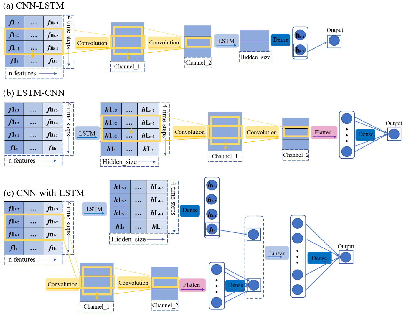
Figure 5 The framework of the proposed CNN and LSTM hybrid models: (a) CNN–LSTM, (b) LSTM–CNN, and (c) CNN-with-LSTM.

LSTM–CNN

In contrast to the CNN–LSTM model, the LSTM–CNN model first utilizes LSTM layers to associate the time series' data and output high-dimensional related hidden states. Subsequently, convolution layers are employed to extract the features of these time-dependent hidden states. This model has also been widely adopted in various applications (Xia et al., 2020). In this study, LSTM–CNN for soil moisture prediction consists of an LSTM layer and two convolution layers sequentially. The structure of LSTM–CNN can be seen in Fig. 5b. The detailed layers and parameters of this model are presented in Table A1.

CNN-with-LSTM

CNN-with-LSTM is a model that employs the parallel combination of both CNN and LSTM, merging their outputs through concatenation, and uses a fully connected network for regression analysis. By combining the feature extraction capabilities of CNN with the time series memory ability of LSTM, this model captures both the local and global temporal characteristics of the input data. This kind of hybrid structure has been used in soil moisture prediction and achieved satisfactory results (Yu et al., 2021). In our work, CNN-with-LSTM is comprised of an LSTM layer and two convolution layers in parallel, and the structure is depicted in Fig. 5c. Table A1 lists the network structures of the CNN and LSTM models in addition to the parameter settings.

3.3.2 Hybrid structure of attention and LSTM

To enhance the accuracy of deep learning models and address the issue of a lack of interpretability, attention mechanisms have been incorporated into LSTM models to weigh the importance of different input and output vector dimensions (Li et al., 2022a; Ding et al., 2020; Xia et al., 2020). Attention mechanisms are commonly used in combination with other neural networks as a form of preprocessing or post-processing. Through training, attention mechanisms dynamically generate spatiotemporal attention importance weights to selectively focus on critical parts of the input or output, as illustrated in Fig. 6. These attention weights enable the model to assign importance to various elements within the input sequence, thus helping to make more accurate predictions. Additionally, these attention weights offer a visualized representation, which provides insights into the sections of the input sequence most essential for a specific prediction. According to the specific roles of the attention mechanisms, the hybrid models can be classified into three categories: FA-LSTM (a feature attention mechanism with LSTM), TA-LSTM (a temporal attention mechanism with LSTM), and FTA-LSTM (an LSTM combines both feature and temporal attention mechanisms). Ding et al. (2020) conducted experiments on these three kind of hybrid models in flood prediction, confirming the effectiveness of incorporating LSTM with attention mechanisms.

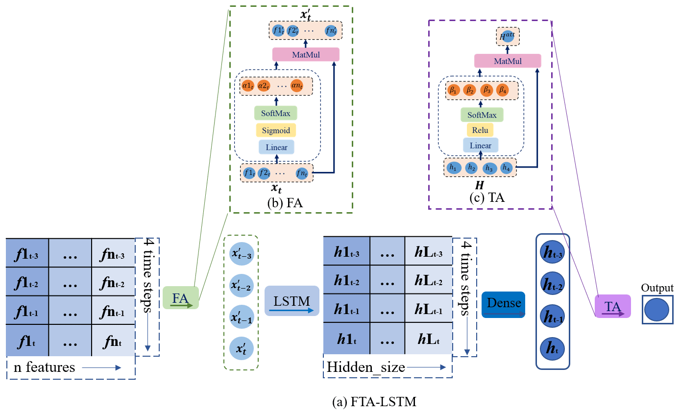
Figure 6 Framework of (a) the proposed FTA-LSTM hybrid models, (b) the feature attention (FA) mechanism, and (c) the temporal attention (TA) mechanism, inspired by Ding et al. (2020).

FA-LSTM

FA-LSTM applies an attention mechanism to assign weights for distinct features in the input vector. In this study, for soil moisture prediction, the feature attention mechanism in FA-LSTM processes the input vector $\mathit{I}\left\{{\mathit{x}}_{t-\mathrm{3}},\mathrm{\dots }{\mathit{x}}_t\right\}$, where ${\mathit{x}}_t=\left\{f{\mathrm{1}}_t,f{\mathrm{2}}_t,\mathrm{\dots }f{n}_t\right\}$ and generates the weighted output $\left\{{\mathit{x}}_{t-\mathrm{3}}{}^{\prime }\mathrm{\dots }{\mathit{x}}_t^{\prime }\right\}$. Through the attention mechanism, the output ${\mathit{x}}_t^{\prime }$ remains the same dimension size as the input x_t. The feature attention importance weight α_t and attention mechanism output ${\mathit{x}}_t^{\prime }$ are defined as follows:

$$\begin{array}{}\text{(12)}& {\displaystyle }{\mathit{\alpha }}_t=\mathrm{FA}\left({\mathit{x}}_t\right),\text{(13)}& {\displaystyle }{\mathit{x}}_t^{\prime }={\mathit{\alpha }}_t\otimes {\mathit{x}}_t.\end{array}$$

Figure 6b also shows the operation of the feature attention mechanism. The FA-LSTM model consists of an LSTM and a feature attention mechanism for input preprocessing, as detailed in Table A1.

TA-LSTM

TA-LSTM utilizes the temporal attention mechanism to weigh the importance of LSTM output vectors across time steps. This enables the model to concentrate on the most relevant hidden states, potentially enhancing its performance on tasks that involve temporal modeling. The temporal attention mechanism is shown in Fig. 6c. In our work, the output vector H^att, which is obtained through the temporal attention mechanism in TA-LSTM, is the weighted sum of all states in $\mathit{H}\left\{{\mathit{h}}_{t-\mathrm{3}},{\mathit{h}}_{t-\mathrm{2}},{\mathit{h}}_{t-\mathrm{1}}{\mathit{h}}_t\right\}$. The temporal attention weight β and attention mechanism output H^att can be defined as follows:

$$\begin{array}{}\text{(14)}& {\displaystyle }\mathit{\beta }=\mathrm{TA}\left(\mathit{H}\right),\text{(15)}& {\displaystyle }{\mathit{H}}^{\mathrm{att}}=\sum _{i=\mathrm{1}}^{\mathrm{4}}{\mathit{\beta }}_{\mathrm{i}}\otimes {\mathit{h}}_{\mathrm{i}}.\end{array}$$

Compared with LSTM, the difference with TA-LSTM lies in the post-processing of the LSTM output. LSTM utilizes the last hidden state output for prediction, whereas TA-LSTM employs temporal weighting to utilize all hidden state outputs. Table A1 contains the network structure and parameters information.

FTA-LSTM

FTA-LSTM is the model that combines both feature and temporal attention mechanisms, as illustrated in Fig. 6a. It applies the feature attention mechanism before the LSTM layer, to assign weights for the input features, and the temporal attention mechanism after the LSTM layer, to weigh the importance of the LSTM output vectors of different time steps. The parameters of FTA-LSTM can be found in Table A1.

3.4 GAN-LSTM

GANs (Goodfellow et al., 2014) comprise a generator and a discriminator. The generator is designed to generate predictions that are similar to the truth, while the discriminator tries to distinguish between the truth and the predictions. The unique network structure and adversarial training of GANs make them highly effective in various fields, particularly in dealing with fuzzy prediction (Jing et al., 2019). Thus, GANs offer a promising way to predict soil moisture, potentially leading to accurate results in real situations. For predicting soil moisture, the GAN-LSTM model is used, where the generator (G) employs an LSTM model capable of processing time series' data, and the discriminator (D) uses a single-layer feedforward neural network, similar to the work of Li et al. (2020). Alternating adversarial training is performed between G and D, meaning that one of them is trained while the other one remains fixed. The structure and training strategies of GAN-LSTM are shown in Fig. 7.

Figure 7 The framework of the proposed GAN-LSTM model.

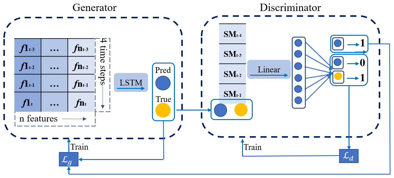
The training objective of the discriminator D is to distinguish between predictions generated by the generator G and the ground truth, by minimizing the loss function L_d. The binary cross-entropy loss is utilized as the similarity evaluation metric, with the objective of training D to output 1 when presented with ground truth as input and 0 when presented with predictions as input:

$$\begin{array}{}\text{(16)}& \begin{array}{rl}{L}_d& =L_{\mathrm{bce}}\left(d\left(\left[{\mathrm{SM}}_{t-\mathrm{4}},\mathrm{\dots },{\mathrm{SM}}_{t-\mathrm{1}},y_t\right]\right),\mathrm{1}\right)\\ & +L_{\mathrm{bce}}\left(d\left(\left[{\mathrm{SM}}_{t-\mathrm{4}},\mathrm{\dots },{\mathrm{SM}}_{t-\mathrm{1}},{\widehat{y}}_t\right]\right),\mathrm{0}\right).\end{array}\end{array}$$

Here, L_bce is the binary cross-entropy loss, which is defined as follows:

$$\begin{array}{}\text{(17)}& L_{\mathrm{bce}}\left(\widehat{p},p\right)=-p\log \left(\widehat{p}\right)-\left(\mathrm{1}-p\right)\log \left(\mathrm{1}-\widehat{p}\right),\end{array}$$

where p denotes the label (0 or 1) and $\widehat{p}$ denotes the logit value between 0 and 1.

For generator G, there are two training objectives: (1) to generate soil moisture dynamics predictions that are accurate and consistent with the truth, which is achieved by minimizing the fitting error of the soil moisture content data, denoted as L_mse; (2) to deceive D, which is achieved by minimizing the binary cross-entropy loss L_bce between the predictions and the truth in D. The output of D should be close to 1 when inputting the G predictions into D, ensuring that the prediction is close to the truth. Therefore, we train G by minimizing the following loss function L_g:

$$\begin{array}{}\text{(18)}& \begin{array}{rl}{L}_g& =L_{\mathrm{mse}}\left(y_t,{\widehat{y}}_t\right)\\ & +{\mathit{\lambda }}_{\mathrm{bce}}{L}_{\mathrm{bce}}\left(d\left(\left[{\mathrm{SM}}_{t-\mathrm{4}},\mathrm{\dots },{\mathrm{SM}}_{t-\mathrm{1}},{\widehat{y}}_t\right]\right),\mathrm{1}\right),\end{array}\end{array}$$

where λ_bce is the hyperparameter that controls the importance of the second term. Here, we determine λ_bce to be $\mathrm{1}\times {\mathrm{10}}^{-\mathrm{7}}$ through manual testing. For adversarial training in our GAN-LSTM, the parameter update ratio of G and D in the model is 3:1; thus, every time G is updated (the learning rate is set to 0.0005), D will be updated three times (the learning rate is set to 0.001). The network structure parameters of GAN-LSTM are recorded in Table A1.

4 Results and discussion

This study evaluates the performance of 3 machine learning methods and 10 deep learning models with respect to predicting soil moisture at 10 sites and 5 depths. To evaluate the model's ability to predict over time series, we examined forecasts for 1, 3, and 7 d ahead. When making predictions longer than 1 d, we adopted iterative predictions. The generated soil moisture data for the first day, along with the corresponding observed meteorological data and historical 3 d data, reconstruct the new 4 d input, which is used to predict soil water for the second day. Two standard metrics, R² and root-mean-square error (RMSE) are used to evaluate the performance of the models. R² represents how well the model captures the variability in the data, whereas the RMSE measures the accuracy of the model's predictions. These metrics are calculated as follows:

$$\begin{array}{}\text{(19)}& {\displaystyle }{R}^{\mathrm{2}}=\mathrm{1}-{\displaystyle \frac{{\sum }_{i=\mathrm{1}}^N{\left(y_i-{\widehat{y}}_{\mathrm{i}}\right)}^{\mathrm{2}}}{{\sum }_{i=\mathrm{1}}^N{\left(y_i-{\overline{y}}_{\mathrm{i}}\right)}^{\mathrm{2}}}},\text{(20)}& {\displaystyle }\mathrm{RMSE}=\sqrt{{\displaystyle \frac{{\sum }_{i=\mathrm{1}}^N{\left(y_i-{\widehat{y}}_{\mathrm{i}}\right)}^{\mathrm{2}}}{N}}}.\end{array}$$

Here, y_i denotes the ground truth, ${\widehat{y}}_{\mathrm{i}}$ denotes the model prediction, ${\overline{y}}_{\mathrm{i}}$ denotes the mean of the ground truth, and N denotes the sample size.

The collected data in Sect. 2 are split into training, validation, and test sets using a $\mathrm{6}:\mathrm{2}:\mathrm{2}$ ratio in time order, as summarized in Appendix D. The training set is used to train the models with a learning rate of 0.001 unless stated otherwise. We train the deep learning models for at least 1500 epochs, with a batch size of 50. In each epoch, 20 batches are used for training. The validation set is employed to determine whether the deep learning model should be updated. If the trained model performs worse on the validation set compared with the previous model, the previous model is retained. Finally, the test set is utilized to evaluate and compare the accuracy of the trained models. To ensure statistical robustness, each final result is obtained by averaging the outcomes of 25 repetitions of the training process.

4.1 Comparisons of machine learning and LSTM

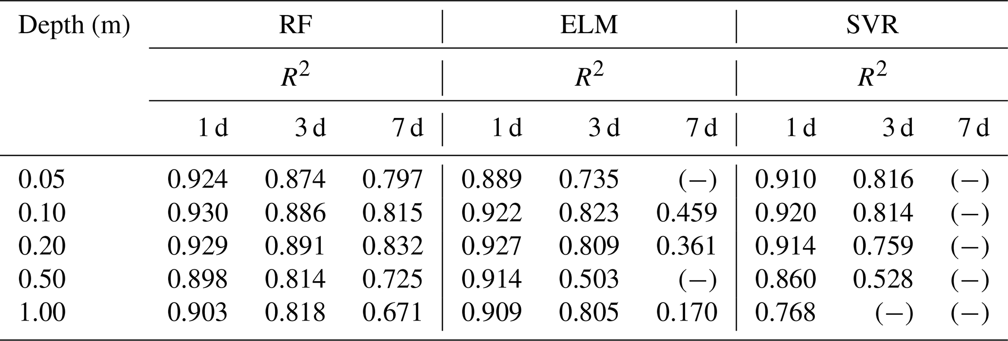
This section compares the machine learning models with the deep learning model, represented by LSTM. Table 2 summarizes the R² between the soil moisture predictions of the three machine learning methods and the ground truth at 10 sites and 5 depths for the following 1, 3, and 7 d. The symbol (−) signifies an extremely poor R² result. The results show that all three methods perform well on short-term (1–3 d) soil moisture forecasts, but their performance tends to diverge when predicting at the lead time of 7 d. Among these three, RF is the most stable and best-performing model.

Figure 8a–e compares the average RMSE of the soil moisture predictions of the machine learning models and LSTM at different depths for 1, 3, and 7 d ahead across 30 sites. It reveals that LSTM outperforms the three machine learning models in terms of prediction accuracy and stability, which suggests that deep learning has a better capability to process time series' data for soil moisture dynamics simulation than traditional machine learning.

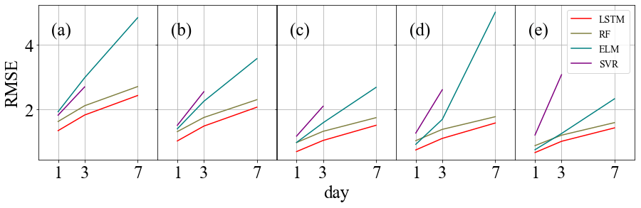
Figure 8 RMSE comparisons between RF, ELM, SVR, and LSTM at the Cape-Charles site at five depths: (a) 0.05 m, (b) 0.10 m, (c) 0.20 m, (d) 0.50 m, and (e) 1.00 m.

Machine learning models are limited in handling inputs from multiple time steps when processing time series' data. Therefore, while they exhibit proficiency in short-term predictions, they may not perform well in long-term prediction tasks and demonstrate comparatively lower accuracy and stability than deep learning models. Nevertheless, a notable advantage of machine learning models is that they require little training time, enabling rapid deployment, which incurs lower computational costs compared with deep learning models.

Table 2 The values of R² between the predictions (1, 3, and 7 d) of RF, ELM, and SVR and the ground truth for 10 sites at 5 depths.

4.2 Comparisons of 1D-CNN, LSTM, and Transformer

In this section, we conduct a comparative analysis of three basic deep learning networks. We evaluate their predictive performance by assessing both predictive accuracy and computational costs. The R² values between the soil moisture predictions generated by the three models and the ground truth across 10 sites and 5 depths are presented in Table 3. Additionally, Fig. 9a–e display the average RMSE values for soil moisture predictions at 30 sites.

Table 3 The values of R² between the predictions (1, 3, and 7 d) generated by CNN, LSTM, and Transformer and the ground truth across 10 sites at 5 depths.

The results reveal that the LSTM model achieves the highest prediction accuracy, followed by the 1D-CNN model and, subsequently, the Transformer model. Notably, LSTM and Transformer are more stable when making 7 d or deep-soil-moisture predictions, while 1D-CNN is better suited for short-term and shallow prediction tasks. This aligns with the inherent characteristics of the three models. In essence, LSTM is designed to model temporal dependencies in sequential data, emphasizing global features. Transformer operates by modeling relationships in input time series without iterations and highlights important features by self-attention weighting. These characteristics prevent overfitting in the LSTM and Transformer models, resulting in stability in weekly predictions. In contrast, 1D-CNN excels at extracting and expressing local features, which facilitates it capturing the connections between subtle feature changes and their corresponding outcomes. This capability allows for adaptation to shallow-soil-moisture prediction tasks with significant variations.

Figure 9g shows the training epochs required for each model, while Fig. 9h illustrates the time taken for 100 epochs. The 1D-CNN model demonstrates the fastest training speed and achieves early convergence. Conversely, LSTM shows slower training speed, which is attributed to its iterations. The Transformer trains quickly but converges at a slower pace than LSTM, resulting in a similar total training time. In summary, although 1D-CNN offers the lowest computational costs, LSTM has been proven to be the most appropriate for soil moisture prediction tasks among the three with the highest accuracy.

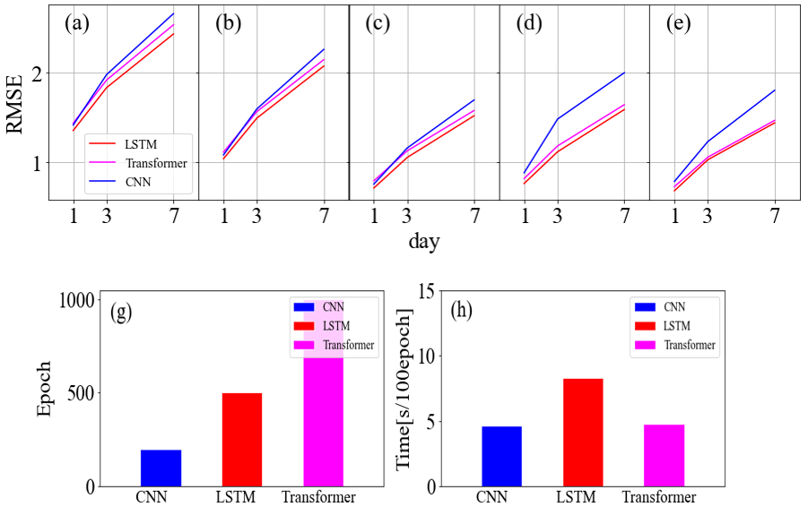
Figure 9 Average RMSE comparisons between CNN, LSTM, and Transformer at five depths: (a) 0.05 m, (b) 0.10 m, (c) 0.20 m, (d) 0.50 m, and (e) 1.00 m. Comparisons of the (g) training epoch and (h) training time for the three models.

4.3 Comparisons of CNN and LSTM hybrid models

This section compares the three CNN and LSTM hybrid models (LSTM–CNN, CNN–LSTM, and CNN-with-LSTM) across 10 sites in terms of prediction accuracy and computational costs. Table 4 presents the R² values between the soil moisture predictions generated by the three hybrid models and the ground truth across 10 sites at 5 depths. It can be observed that the prediction accuracy of these models is comparable, with LSTM–CNN slightly outperforming the others. Moreover, Fig. 10a–e show the average RMSE results of the hybrid models and LSTM across the 30 research sites, indicating that the hybrid models do not exhibit obvious advantages over the standard LSTM.

Table 4 The values of R² between the predictions (1, 3, and 7 d) of LSTM–CNN, CNN–LSTM, and CNN-with-LSTM and the ground truth for 10 sites at 5 depths.

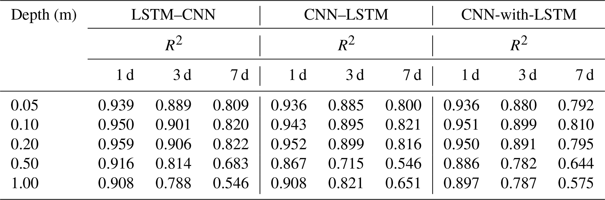
Specifically, the three models are hybrids of CNN and LSTM with varying incorporation degrees. According to their combination methods, we can infer that the models excel with respect to handling different types of data and place different emphases on data characteristics. CNN–LSTM appears to prioritize local features and model long-distance dependencies, whereas LSTM–CNN focuses on global features and context information. CNN-with-LSTM simultaneously considers both local features and temporal information for predictions. These integrations increase the complexity and enhance the expression capacities of models, but their applications should depend on the input data and prediction task. In the case of soil moisture prediction, the benefits of this combination approach are not significant.

Figure 10g and h display the computational costs of the three hybrid models. It is evident that CNN–LSTM shows the fastest training speed and the lowest computational costs, owing to its convolution layers for input data preprocessing. Moreover, the computational costs of LSTM–CNN are higher than CNN-with-LSTM. Overall, compared with LSTM and 1D-CNN, we could draw the conclusion that the hybrid models have limited practical value in soil moisture prediction.

Figure 10 Average RMSE comparisons between LSTM–CNN, CNN–LSTM, and CNN-with-LSTM at five depths: 0.05 m (a), 0.10 m (b), 0.20 m (c), 0.50 m (d), and 1.00 m (e). Comparisons of the training epoch (g) and training time (h) for the three models.

4.4 Comparisons of attention mechanisms and LSTM hybrid models

To investigate the impact of different attention mechanisms on models, this section compares these three models: FA-LSTM, TA-LSTM, and FTA-LSTM. Figure 11a–e display the average RMSE values of the soil moisture predictions for 1, 3, and 7 d ahead generated by these three models and the standard LSTM at the 30 sites. Table 5 records the R² values between the soil moisture predictions of three models and the ground truth across 10 sites and 5 depths.

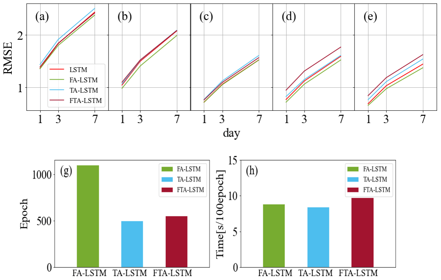
Figure 11 Average RMSE comparisons between FA-LSTM, TA-LSTM, and FTA-LSTM at five depths: 0.05 m (a), 0.10 m (b), 0.20 m (c), 0.50 m (d), 1.00 m (e). Comparisons of the training epoch (g) and training time (h) for the three models.

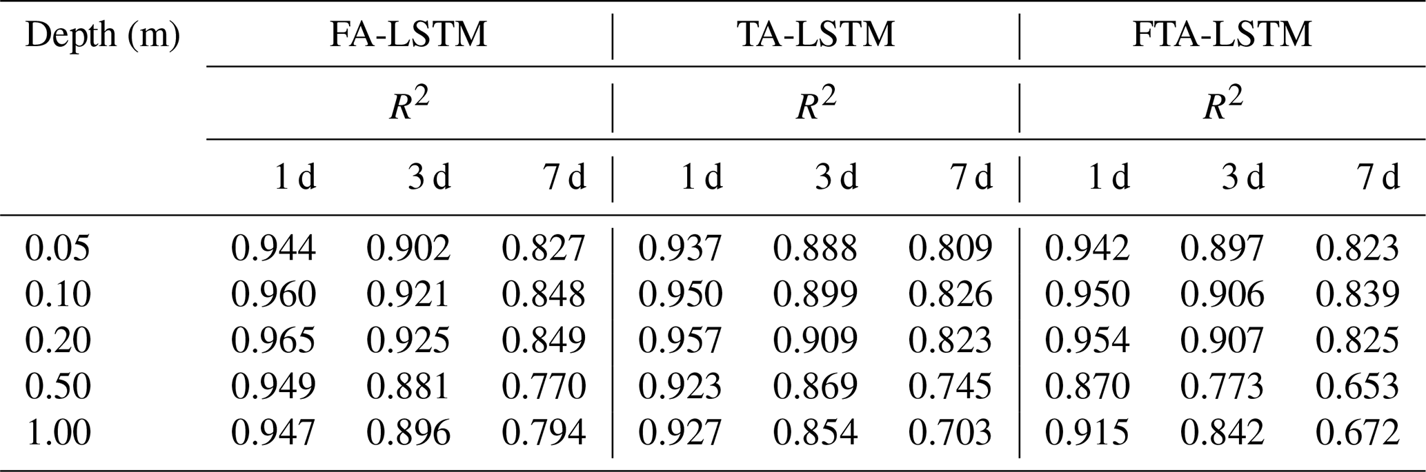
Table 5 The values of R² between the predictions (1, 3, and 7 d) of FA-LSTM, TA-LSTM, and FTA-LSTM and the ground truth for 10 sites at 5 depths.

Based on the results, the prediction accuracy of the three models ranked from high to low is FA-LSTM, FTA-LSTM, and TA-LSTM in most situations. It can be found that the feature attention mechanism has a stable gain effect on LSTM, potentially because it assigns the appropriate feature importance weights to various influencing factors, especially in deep-soil-moisture prediction tasks. On the contrary, the improvement in the temporal attention mechanism is not evident and may lead to deterioration. TA-LSTM differs from LSTM in its output post-processing, as it is trained to weigh the LSTM output at each time step to make predictions. The reason why TA-LSTM is worse may be that LSTM already encodes enough past features for predictions in the last hidden state. Moreover, the FTA-LSTM model, which combines both feature and temporal attention mechanisms, is the most complex but not necessarily the optimal model among the three. From the results, we can also infer the effective feature learning ability of attention mechanisms.

According to Fig. 11g–h, attention mechanisms introduce some acceptable computational costs. Notably, FA-LSTM requires more training steps to reach convergence. However, despite this computational requirement, we believe that the implementation of FA-LSTM is still advantageous for soil moisture prediction tasks.

Figure 12 provides visualizations of the input feature importance and temporal importance weights learned by FA-LSTM and TA-LSTM for soil moisture prediction at the AAMU-jtg site across five depths. The feature importance in Fig. 12a–e shows a reasonable adaptation to the varying depth, demonstrating the effective feature selection capability of attention mechanisms. Moreover, the temporal importance in Fig. 12f–j indicates the high utilization of recent temporal features, which is consistent with real situations. This indicates the effective feature learning capacity of attention mechanisms. Moreover, these results contribute to a deeper understanding of the utilization mechanisms of feature and temporal information within the model.

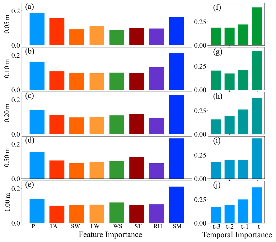
Figure 12 Feature importance and temporal importance for soil moisture prediction at the AAMU-jtg site across five depths.

4.5 Comparisons of GAN-LSTM and LSTM

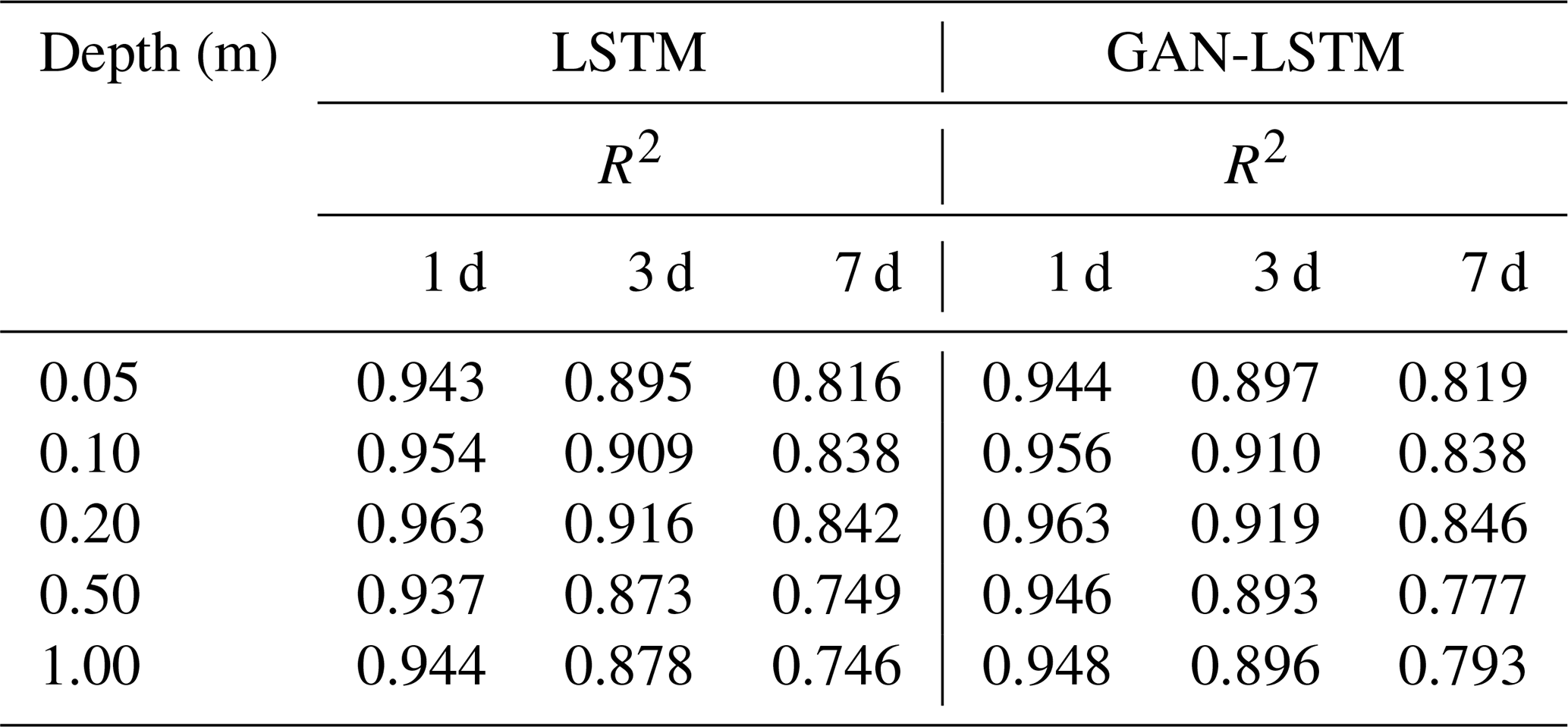
In this section, we evaluate the impact of the GAN structure and adversarial training strategy on the standard LSTM model. LSTM and GAN-LSTM for soil moisture prediction are compared. The R² values for the following 1, 3, and 7 d across 10 sites at different depths are recorded in Table 6. Figure 13a–e show the RMSE results of LSTM and GAN-LSTM at the Weslaco site.

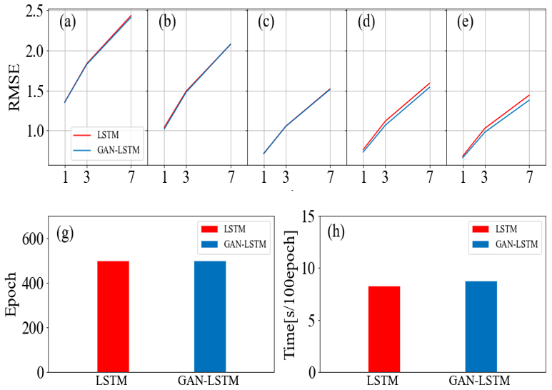
Figure 13 Average RMSE comparisons between LSTM and GAN-LSTM at five depths: 0.05 m (a), 0.10 m (b), 0.20 m (c), 0.50 m (d), and 1.00 m (e). Comparisons of the training epoch (g) and training time (h).

The results demonstrate that GAN-LSTM achieves better performance than the standard LSTM in most situations, particularly in 3–7 d prediction tasks. The application of the GAN structure and training strategies enhances the prediction accuracy of LSTM. The adversarial training of GAN-LSTM allows the model to not only learn from the data but also extract additional information embedded in the data. This helps address performance degradations due to overfitting on the data mean-square error. We can regard this training strategy as a general principle to enhance the performance of neural networks. However, the selection of hyperparameters in the loss function of GAN is crucial and currently requires manual adjustments. In future work, adaptive methods can be adopted to automatically adjust the GAN-LSTM loss function to increase training flexibility and prediction accuracy.

Table 6 The R² values between the predictions (1, 3, and 7 d) generated by LSTM and GAN-LSTM and the ground truth across 10 sites at 5 depths.

Based on the computational cost comparisons presented in Fig. 13g–h, both LSTM and GAN-LSTM exhibit similar computational costs. Consequently, in most scenarios, it is advisable to apply the GAN-LSTM model to predict soil moisture dynamics. It improves the stability and prediction ability of the model without imposing a significant increase in computational costs.

4.6 Visualization analysis

In this study, we employ the SHAP method (Lundberg et al., 2018) to quantify the contributions of input features to investigate the distinct mechanisms of data utilization in different network structures. Brief introductions to SHAP are provided in Appendix B. Figure 14 illustrates the SHAP summary plots of these 10 deep learning models utilizing samples from the test set of the Monahans-6-ENE site. The y axis represents the input features ranked by importance. Each point shows the Shapley value of a specific feature in a sample, with the color indicating the value of the input feature. The plot clearly shows the identified main influential factors and established correlations between input features and soil moisture by the models. We aim to analyze different ways of using data across various models. For soil moisture predictions, a SHAP analysis visualization for a high-performing model should reflect its emphasis on influential features for improved results in surface soil moisture or short-term predictions. Simultaneously, it can illustrate the model's capability to avoid overlearning irrelevant features. This avoidance can prevent false correlations that can degrade long-term forecast performance.

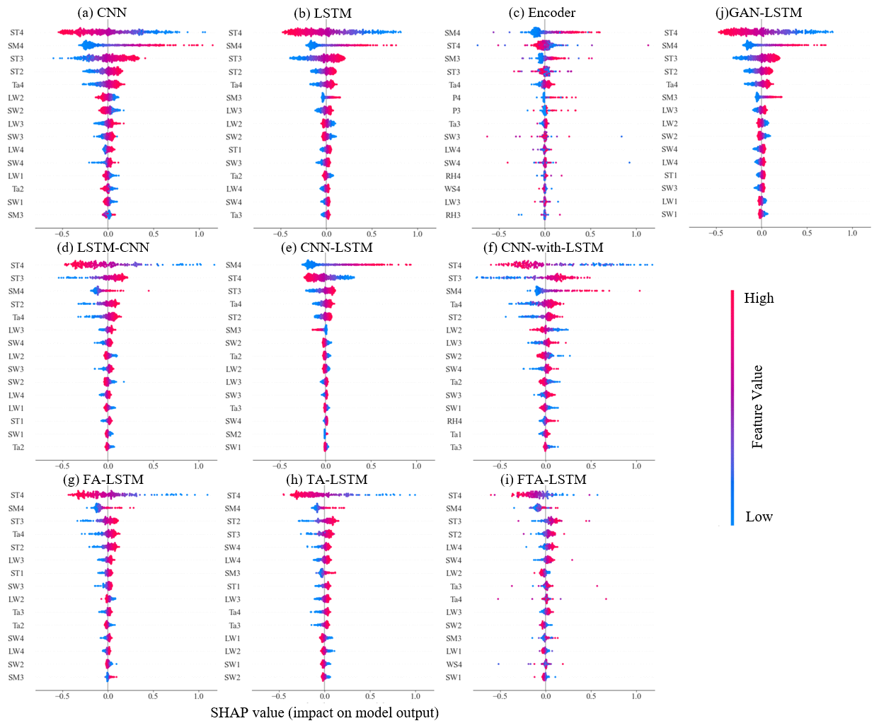
Figure 14 SHAP summary plots for 10 deep learning models. The samples are from the test set of the Monahans-6-ENE site at 0.05 m.

Figure 14a–c display the Shapley values of three basic deep learning models: CNN, LSTM, and Transformer. It can be observed that CNN shows a broader range of Shapley values compared with the others, indicating its greater feature expression capacity. This suggests that CNN focuses more on specific local features, whereas LSTM emphasizes capturing global features. However, both CNN and LSTM tend to learn incorrect correlations. For instance, the learned positive correlation between the feature ST3 and soil moisture is contrary to the facts. The Transformer model, which aggregates features from all other inputs, appears to perform better in this aspect. Although the Shapley value of the Transformer exhibits the lowest range, the important features identified are derived from the recent input time series, which aligns better with real situations. This reflects the effective feature learning ability of attention mechanisms. Overall, each of these models – CNN, LSTM, and Transformer – possesses unique advantages in terms of data utilization. Notably, LSTM aligns most consistently with the above criteria.

Figure 14d–f compare the hybrid models of CNN and LSTM models. The CNN–LSTM keeps high Shapley values in important features while showing minimal response to the others. This suggests that CNN–LSTM tends to sequentially process the extracted crucial features, enabling itself to effectively capture both local data features and long-range dependencies, more closely resembling the CNN. LSTM–CNN shows similar Shapley values to LSTM. By employing CNN to extract sequential modeling features, LSTM–CNN emphases global features more, resembling the characteristics of the LSTM. The Shapley value of the CNN-with-LSTM is the highest, displaying a heightened sensitivity to feature perturbations. This can be attributed to the repeated utilization of features in parallel networks. These three models represent different degrees of fusion between CNN and LSTM models, and the hybrid architecture design depends on the specific task requirements and data characteristics.

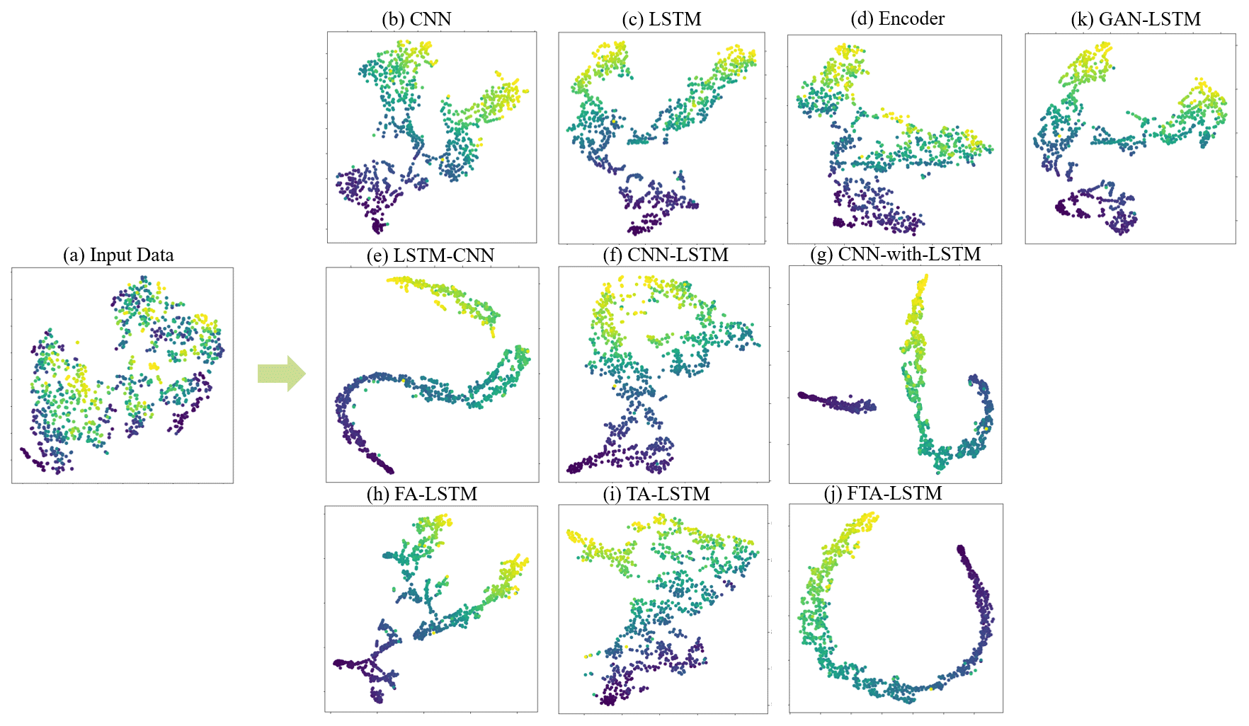
Figure 15 The t-SNE visualizations of the original input data (a) and encoded hidden states of 10 models (b–k) obtained from the LittleRiver site test set. The colors of the points indicate the corresponding soil moisture content values.

In the case of hybrid models that integrate attention mechanisms with LSTM, FA-LSTM, TA-LSTM, and FTA-LSTM, their Shapley values in Fig. 14g–i are found to differ slightly from that of LSTM. Considering the attention importance analysis discussed in Sect. 4.4, we can infer that the attention mechanisms introduce slight adjustments to the time and feature attributions on the basis of the LSTM. Figure 14j also presents the Shapley value of GAN-LSTM. Through the Shapley value, we can infer that the GAN-LSTM model introduces slight modifications during adversarial training, influencing some feature contributions to improve the prediction accuracy of the LSTM model. This demonstrates that adversarial training strategies contribute to the refinement and enhancement of models.

Besides, t-SNE (Van der Maaten and Hinton, 2008), a dimension reduction and visualization method is employed to discover the structure and patterns in the high-dimensional data. When mapping data onto a two-dimensional space, t-SNE retains the relative distance relationships between the original data points, ensuring that similar samples are mapped closer to each other. The details of t-SNE can be found in Appendix B. Figure 15 presents the t-SNE visualizations of the input data and the last encoded hidden states from 10 models. The input data in Fig. 15a denotes the flattened form of the inputs I for the 4 d. When conducting t-SNE visualizations, the x and y axes make no sense. Only the relative distance between sample points matters. The color of each point corresponds to the soil moisture content value. It is evident that, through training, the low-dimensional embeddings of the encoded hidden states gradually transition from an initially irregular pattern to a more structured shape. However, the visualization shapes vary across the different models. For a soil moisture prediction regression task, we discover that the sample points can be arranged vertically from light to dark in color in t-SNE visualizations of models with great forecasting capacity, such as the Fig. 15h. Additionally, these visualizations enable us to discern the impact of the attention mechanism and adversarial training on LSTM in Fig. 15k–h, ultimately leading to enhanced accuracy. However, LSTM–CNN, CNN-with-LSTM, and FTA-LSTM exhibit distinct clustering patterns in their embedding plots, rather than a vertical arrangement. This reflects their advanced data processing capabilities but is less beneficial for soil water prediction tasks. Generally, from the t-SNE visualizations, it can be summarized that different deep learning models capture distinct intrinsic characteristics of input data and encode them into various vectors for making predictions. To gain a more comprehensive understanding of their differences, further research is warranted in the future.

5 Conclusions

In this research, we have conducted a comprehensive analysis of traditional machine learning models and various deep learning models for soil moisture predictions across different sites at five depths. Based on our comparisons of these models, we draw the conclusions outlined in the following.

In traditional machine learning, RF seems to be the most stable method in soil moisture prediction tasks. However, deep learning models have been found to possess stronger capabilities with respect to processing time series' data for better predictions. Among the three basic deep learning models, LSTM demonstrates a high level of accuracy because of its temporal information modeling capability, while 1D-CNN exhibits the lowest computational cost. Transformer also shows a stable weekly forecasting ability. When considering the hybrid models, three combinations of CNN and LSTM did not enhance the prediction abilities in this task. Despite the attractiveness of hybridizing the benefits of CNN and LSTM, the results did not find notable advantages for soil moisture prediction in terms of accuracy and computational costs. However, the feature attention mechanism has a constant positive effect on LSTM, whereas temporal attention mechanisms have little significance. In addition, incorporating generative adversarial network structures and training strategies into LSTM models (GAN-LSTM) has been found to improve prediction accuracy, especially in 7 d predictions. To summarize, FA-LSTM and GAN-LSTM are found to be the most stable and effective models for soil moisture prediction. Furthermore, this study attempts to provide a thorough analysis of models' performance and advance the understanding of machine learning in soil moisture prediction. Through the Shapley analysis, we can infer the different data utilization methods of the 10 models. Furthermore, the t-SNE visualizations illustrate the varying encoding capabilities of different models.

The results emphasize the importance of appropriate and effective neural network structure design for a given task. For soil moisture prediction, several principles of effective network design can be concluded. Firstly, leveraging the temporal modeling capability of LSTM is well suited for soil moisture forecasting. Secondly, incorporating attention mechanisms properly facilitates efficient feature learning. The feature selection capability of attention mechanisms has been proven through the performance of the Transformer and the attention mechanisms and LSTM hybrid models. Lastly, applying special GAN structures and adversarial training strategies in models helps extract additional information embedded within data, which could also potentially improve soil moisture dynamics simulation.

This study provides a reference and lays the groundwork for the development of specialized deep learning models for soil moisture dynamics simulation. However, although data-driven models have shown satisfactory performance, they cannot make long-term predictions precisely due to their lack of physical laws. In the future, the integration of known physical laws with deep learning models will become a promising research direction for soil moisture dynamics simulation.

Appendix A: Parameters used in machine learning and deep learning models

Table A1 Parameters settings of the deep learning models.

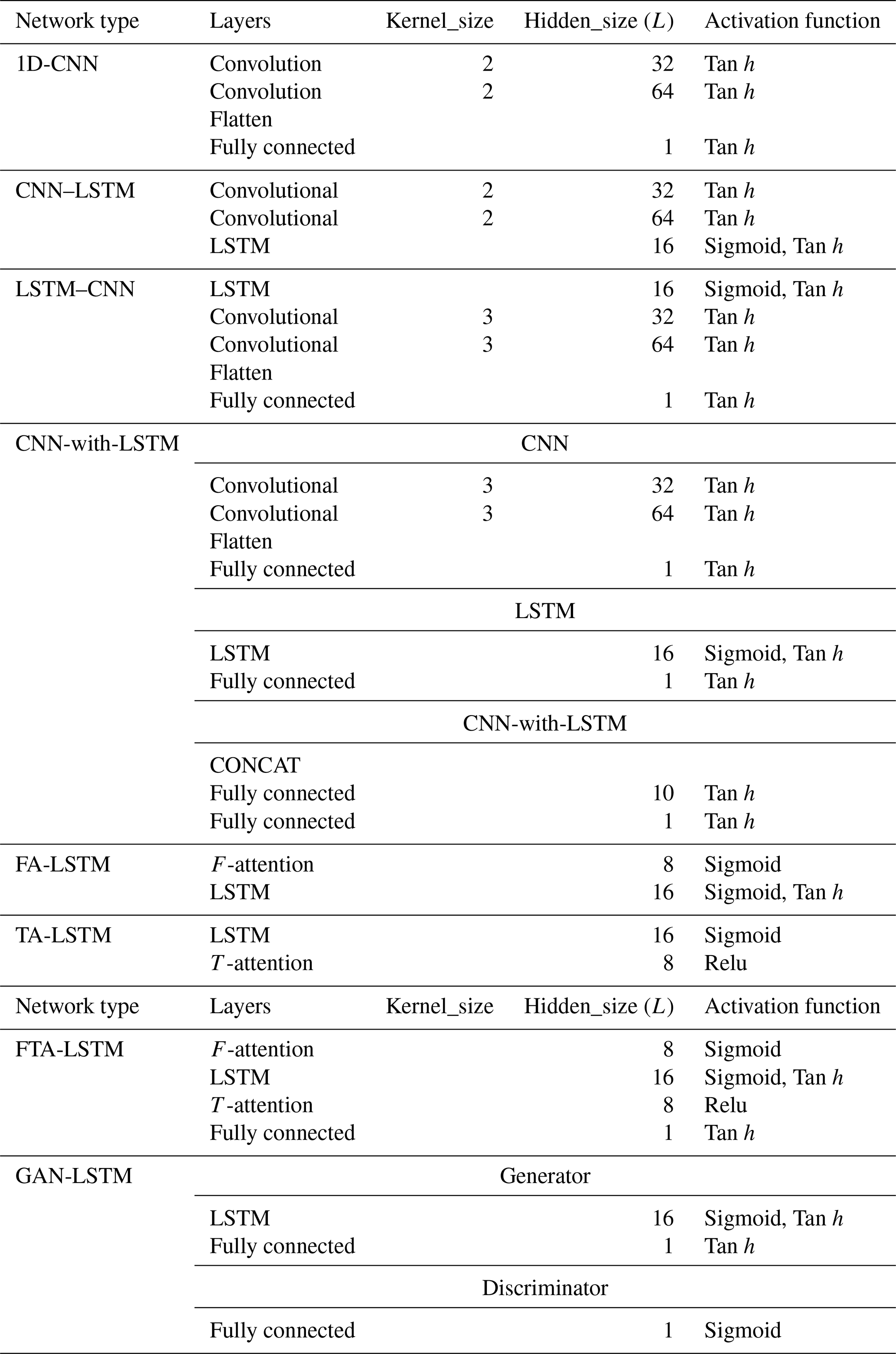
RF: the default parameter values in RandomForestRegressor of the scikit-learn library. SVR: C= 1.0, ε= 0.1, kernel γ= “poly”. ELM: Hidden_size (L) = 20. LSTM: num_layers = 2, Hidden_size (L) = 16. Transformer: d_k = d_v = 4, d_model = feature = 8, d_ ff = 20, n_heads = 1.

Appendix B: Shapley additive explanations (SHAP)

SHAP (Lundberg et al., 2018) is a game theory approach to explain the output of machine learning models. It measures the impact of the input feature on the prediction of an individual sample. SHAP employs the additive feature attribution method to provide a specific explanation:

$$\begin{array}{}\text{(B1)}& f\left(x\right)=g\left(x{}^{\prime }\right)={\mathit{\varphi }}_{\mathrm{0}}+\sum _{i=\mathrm{1}}^M{\mathit{\varphi }}_{i}x{}^{\prime },\end{array}$$

where f(x) denotes the original model; g(x) represents the explanation model with simplified input $x{}^{\prime },x{}^{\prime }\in {\left\{\mathrm{0},\mathrm{1}\right\}}^M$; M is the number of input features; through a mapping function, $x=h_x\left(x{}^{\prime }\right)$; and ϕ_i denotes the feature attribution of feature i. The explanation model g has a unique solution:

$$\begin{array}{}\text{(B2)}& {\mathit{\varphi }}_i\left(f,x\right)=\sum _{z{}^{\prime }\subseteq x{}^{\prime }}{\displaystyle \frac{\left|z{}^{\prime }\right|\mathrm{!}\left(M-\left|z{}^{\prime }\right|-\mathrm{1}\right)\mathrm{!}}{M\mathrm{!}}}\left[f_x\left(z{}^{\prime }\right)-f_x\left(z{}^{\prime }\backslash i\right)\right],\end{array}$$

where |z^′| is the nonzero entry number in z^′, $z{}^{\prime }\subseteq x{}^{\prime }$; $f\left(x{}^{\prime }\right)=f\left(h_x\left(z{}^{\prime }\right)\right)=E\left[f\left(z\right)\mathrm{|}{z}_s\right]$; and S denotes the nonzero indexes set in z^′.

Appendix C: The t-distributed stochastic neighbor embedding (t-SNE) visualization

The t-SNE is a nonlinear dimension reduction technique that assumes the presence of a low-dimensional nonlinear manifold within the high-dimensional data. Its primary task is to bring similar neighboring points close together in the low-dimensional representation. The working process of t-SNE can be divided into several steps: (1) calculate the similarity between data points in high-dimensional space and then (2) calculate the corresponding probability of points in low-dimensional space. The similarity of points is calculated as conditional probability. If readers are interested, more information can be found in the work of Van der Maaten and Hinton (2008). The following outlines the formulae for calculating the respective similarity P_ij and probability q_ij of the points. The similarity between data points in high-dimensional space is given by

$$\begin{array}{}\text{(C1)}& P_{ij}=\left(P_{j\mathrm{|}i}+P_{i\mathrm{|}j}\right)/\mathrm{2}N.\end{array}$$

The corresponding probability of points in low-dimensional space is given by

$$\begin{array}{}\text{(C2)}& q_{ij}={\displaystyle \frac{{\left(\mathrm{1}+{∥y_i-y_j∥}^{\mathrm{2}}\right)}^{-\mathrm{1}}}{{\sum }_{k\ne l}{\left(\mathrm{1}+{∥y_k-y_l∥}^{\mathrm{2}}\right)}^{-\mathrm{1}}}}.\end{array}$$

Here, P_i|j denotes the conditional probability of point i picking point j as its neighbor if neighbors are chosen according to their probability density under a Gaussian distribution centered at i, N denotes the data points number, y_i denotes the low-dimensional representation of point i, and ∥y_i−y_j∥ denotes the Euclidean distance between y_i and y_j.

Appendix D: Detailed meteorological information on the research sites

The soil moisture time series' data and detailed meteorological information are recorded in this Appendix.

Figure D1 Soil moisture content time series' data at various depths for the 30 sites.

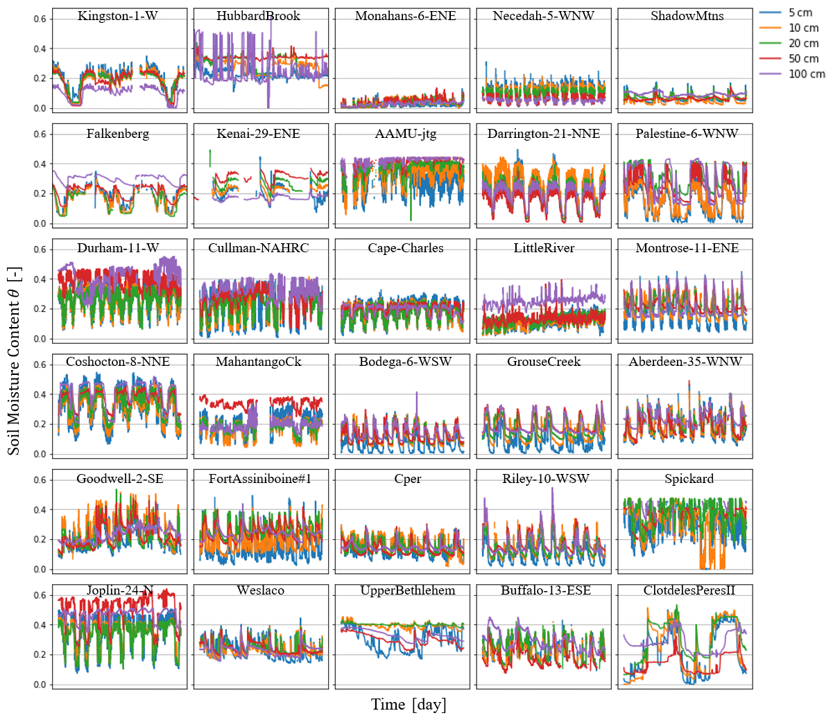
Table D1 Statistical results of P and TA at the 30 sites.

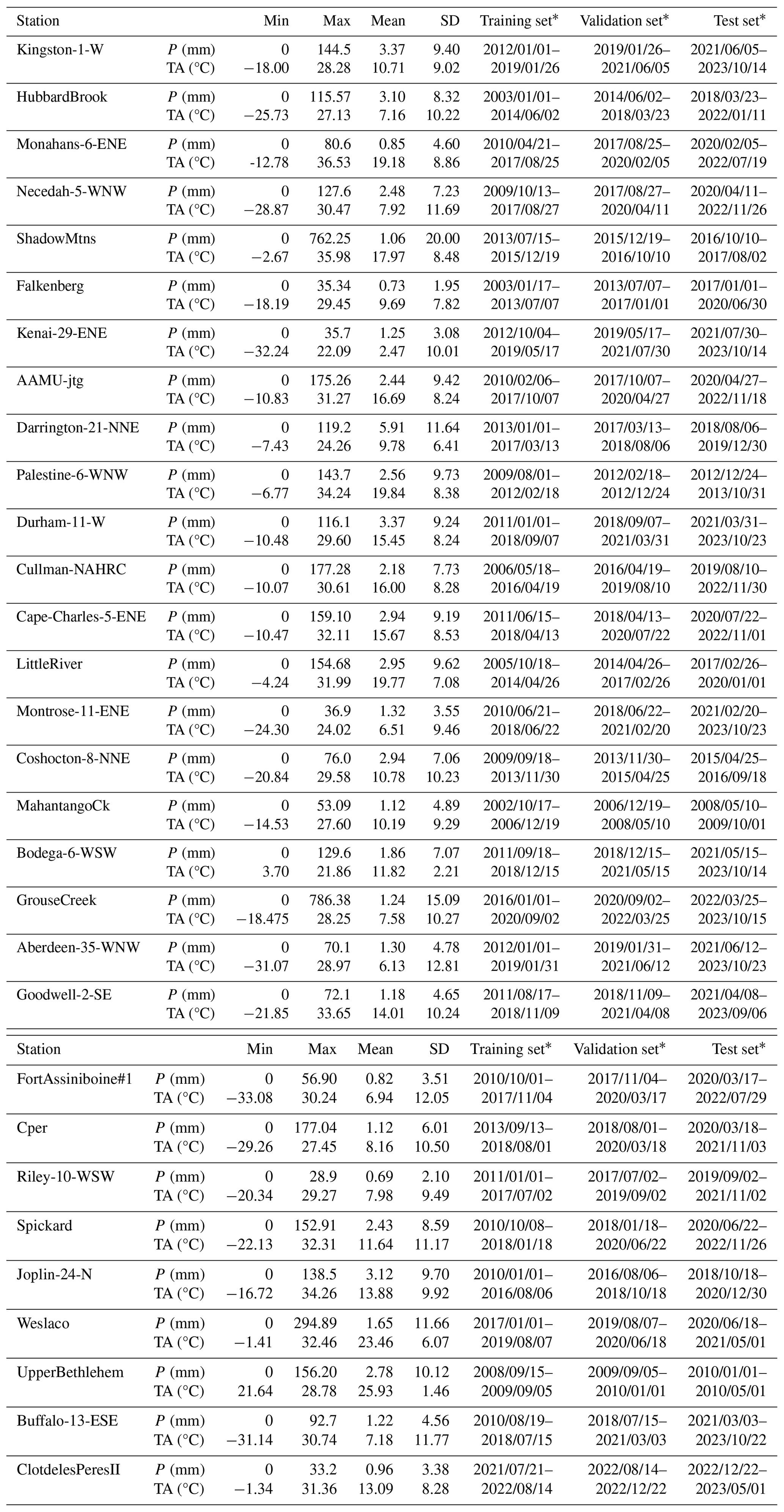
^* Please note that dates are given in the following format: year/month/day.