Past, present and future rainfall erosivity in central Europe based on convection-permitting climate simulations

Heavy rainfall is the main driver of soil erosion by water, which is a threat to soil and water resources across the globe. As a consequence of climate change, precipitation – especially extreme precipitation – is increasing in a warmer world, leading to an increase in rainfall erosivity. However, conventional global climate models struggle to represent extreme rain events and cannot provide precipitation data at the high spatiotemporal resolution that is needed for an accurate estimation of future rainfall erosivity. Convection-permitting simulations (CPSs), on the other hand, provide high-resolution precipitation data and a better representation of extreme rain events, but they are mostly limited to relatively small spatial extents and short time periods. Here, we present, for the first time, rainfall erosivity in a large modeling domain such as central Europe based on high-resolution CPS climate data generated with the regional climate model COSMO-CLM using the Representative Concentration Pathway 8.5 (RCP8.5) emission scenario. We calculated rainfall erosivity for the past (1971–2000), present (2001–2019), near future (2031–2060) and far future (2071–2100). Our results showed that future increases in rainfall erosivity in central Europe can be up to 84 % in the region's river basins. These increases are much higher than previously estimated based on regression with mean annual precipitation. We conclude that despite remaining limitations, CPSs have an enormous and currently unexploited potential for climate impact studies on soil erosion. Thus, the soil erosion modeling community should closely follow the recent and future advances in climate modeling to take advantage of new CPSs for climate impact studies.

1 Introduction

Soil erosion by water is one of the main threats to soils worldwide (Amundson et al., 2015; Panagos et al., 2015a). It causes severe ecological and socioeconomic problems such as ecosystem degradation (Bilotta and Brazier, 2008; Orgiazzi and Panagos, 2018; Mueller et al., 2020; Stefanidis et al., 2022), loss of fertile topsoil on agricultural land (Pimentel et al., 1995; Zhao et al., 2013; Sartori et al., 2019), channel and reservoir siltation (Wisser et al., 2013; Kondolf et al., 2014), and nutrient and contaminant transport to waterbodies (Owens et al., 2005; Ciszewski and Grygar, 2016). Heavy rainfall is the main driving force of soil erosion by water. It acts via the detachment of soil particles by raindrop impact or shear forces of overland flow and subsequent transport of soil particles with overland flow. Rainfall erosivity was first quantified in the 1950s and can be defined as “the capability of rainfall to cause soil loss from hillslopes by water” (Nearing et al., 2017). It is most commonly expressed as the R factor of the Universal Soil Loss Equation (USLE; Wischmeier and Smith, 1978) and its revised versions RUSLE (Renard et al., 1993) and RUSLE2 (USDA Agricultural Research Service, 2008). The USLE, its different versions and models based on the USLE are the most widely used soil erosion models (Borrelli et al., 2021). The USLE calculates average annual soil loss at a site from rainfall erosivity, soil erodibility, topography, crop management and control practices.

Rainfall erosivity is governed by rainfall kinetic energy, which itself depends on raindrop numbers, sizes and fall velocities (e.g., Laws and Parsons, 1943; Wilken et al., 2018). As drop size distributions and fall velocity distributions are usually not available for long periods of time and large study sites, rainfall intensity is usually used as a proxy. Numerous kinetic energy–rainfall intensity relations exist in the literature and are used in soil erosion modeling (Van Dijk et al., 2002; Wilken et al., 2018; Brychta et al., 2022). Site-specific rainfall erosivity expressed as the USLE R factor is commonly calculated from long-lasting precipitation records from rain gauges. The suitability of R-factor equations to represent rainfall erosivity depends strongly on the temporal resolution of the underlying precipitation data time series. R factors decrease with decreasing resolution of the precipitation data because intensity peaks are reduced when precipitation is aggregated over longer time spans (Fischer et al., 2018). When high-resolution precipitation data are only available at a few locations or for limited time periods but low-resolution data (daily–annual) are available elsewhere (e.g., denser rain gauge networks, past reconstructions or future projections), so-called low-resolution approaches can be applied (Brychta et al., 2022). These approaches are based on empirical relations between rainfall erosivity calculated from high-resolution data and lower-resolution rainfall amounts (usually monthly, seasonal or annual totals). Application of these approaches to calculate future changes in rainfall erosivity is not permitted if the frequency distribution of rainfall events changes, as expected under climate change.

Erosion modeling usually requires contiguous data of rainfall erosivity which is highly variable in space (Auerswald et al., 2019a). This spatial variability is usually not represented by rain gauge networks, so spatially interpolated raster data are necessary. Gauge-adjusted radar rainfall data have a high potential for the estimation of highly resolved and contiguous rainfall erosivity maps (Fischer et al., 2018; Risal et al., 2018; Auerswald et al., 2019a; Kreklow et al., 2020). Where ground-based radar data are not available, satellite-based gridded precipitation data sets can also be used to generate contiguous maps (Vrieling et al., 2010; Teng et al., 2017; Phinzi and Ngetar, 2019).

Globally, precipitation is increasing due to an increase in atmospheric water vapor in warmer air (e.g., Allan et al., 2020; Fowler et al., 2021). For central Europe, a net increase in total precipitation is projected with a decrease in summer and an increase in winter (Brienen et al., 2020; Jacob et al., 2014). Furthermore, warming and higher atmospheric moisture fluxes lead to an intensification of the water cycle, causing an increase in the intensity and frequency of extreme precipitation, globally as well as in central Europe (Allan et al., 2020; Brienen et al., 2020; Fowler et al., 2021). Strong increases in extreme precipitation are due to the fact that the share of convective precipitation in total precipitation is increasing (Berg et al., 2013). Trends of an increase in the frequency and intensity of extreme precipitation have been observed since the beginning of the 20th century (Groisman et al., 2005; Alexander et al., 2006; Arnone et al., 2013; Kendon et al., 2014; Fischer and Knutti, 2016) and are expected to continue in the future (Allen and Ingram, 2002; Kharin et al., 2013; Scoccimarro et al., 2013; Westra et al., 2013, 2014; Kendon et al., 2017; Fowler et al., 2021). Thus, rainfall erosivity and soil erosion have also been observed to increase and are expected to increase further (Nearing et al., 2004; Mueller and Pfister, 2011; Hanel et al., 2016a; Panagos et al., 2017, 2022; Auerswald et al., 2019a, b; Borrelli et al., 2020).

For climate impact studies on soil erosion, a common limitation is the lack of reliable high-resolution precipitation data for the future (Eekhout and De Vente, 2020). Projections of future precipitation from regional climate models in Europe are typically available at a temporal resolution of 1 d and a spatial resolution of 0.11^∘ (approx. 12 km) (e.g., Jacob et al., 2014). Thus, low-resolution approaches based on regression models that estimate future R factors from monthly or annual precipitation are commonly applied (Eekhout and De Vente, 2020). Out of 68 climate impact assessment studies reviewed by Eekhout and De Vente (2020), only 4 used sub-daily precipitation data. In the review of 3030 soil erosion modeling studies by Borrelli et al. (2021), 196 were identified to have the aim to model “climate change” or “land use change and climate change” impacts. Only 11 out of the 196 studies are quoted to use sub-daily precipitation data. The few studies that use hourly or sub-hourly future precipitation data mostly use either statistical downscaling of lower-resolution data (Routschek et al., 2015; Wang et al., 2018) or artificially generated precipitation time series (e.g., Coulthard et al., 2012; Simonneaux et al., 2015). Strictly speaking, regression-based models applying monthly or annual precipitation are only valid for the time period for which these models are calibrated and lead to underestimations of the rainfall erosivity if extreme precipitation events increase with time, as suggested by many climate change scenarios.

Only recently, the development of convection-permitting simulations (CPSs) has offered the possibility to model rain erosivity considering the effects of a changing frequency of heavy precipitation that predominantly drives future soil erosion. Thus, CPSs have an enormous and currently unexploited potential for the calculation of future rainfall erosivity. CPSs are performed with regional climate models (RCMs) at a high spatial resolution (usually ≤ 4 km). Due to the coarse resolution of conventional climate simulations, deep convection has to be parameterized as a sub-grid-scale process, which leads to deficits in the realistic simulation of precipitation. This parameterization is switched off in the model setup of a CPS (Lucas-Picher et al., 2021), allowing the model to simulate the precipitation explicitly in each grid cell. A good representation of deep convection is crucial, as it is the main source of precipitation in many parts of the world and is especially important because it often generates extreme precipitation (Prein et al., 2015). As the grid size of most CPSs still ranges between 2 and 4 km, large deep convection cells are explicitly simulated, while smaller shallow convection still needs to be simulated using a parameterization. Despite this shortcoming, CPSs provide an improved representation of extreme precipitation compared with climate models with parameterized deep convection. This is due to several improvements: the diurnal cycle is strongly improved (Ban et al., 2014; Prein et al., 2015), the return periods of extreme precipitation are better represented (Rybka et al., 2022) and added value diagnostics have been applied for the comparison to coarse climate model data (Raffa et al., 2021). However, CPSs also show some limitations: simulations at the kilometer scale for regional domains are still time-consuming and they need a considerable amount of computing power. Compromises have to be made: either the covered time period is shortened or the model domain is restricted to the region of interest. Until some years ago, only single CPSs were performed, covering only one future scenario. Thus, given the novelty of CPSs, model ensembles are not yet available for regional model domains, for the length of the time series needed for the robust estimation of rainfall erosivity (∼ 20 years) or for several emission scenarios. Lately, first-of-their-kind CPS ensembles have been created through combined efforts in the CPS community (Coppola et al., 2020; Ban et al., 2021). Even though these ensemble simulations do not yet cover the long time periods needed for the estimation of rainfall erosivity, these flagship studies show promising results which suggest that ensembles of CPSs will be available for climate impact studies including studies on soil erosion in the future.

The COSMO-CLM is a regional climate model that is used on horizontal scales from 1 to 50 km (Rockel et al., 2008). It is the climate version of the former operational forecast model of the Consortium for Small-scale Modeling (COSMO) of the German meteorological service (Deutscher Wetterdienst, DWD) and other European partners. COSMO-CLM is jointly maintained and developed by the climate limited-area modeling (CLM) community (CLM-Community) but will soon be gradually replaced by the newly developed regional climate model ICON-CLM (Pham et al., 2021). In the framework of the BMDV Expertennetzwerk project, CPSs have been performed with COSMO-CLM. Three time periods, including one historical period (1971–2000, called CPS-hist) and two future periods (CPS-scen, near future: 2031–2060; far future, 2071–2100), were simulated by dynamically downscaling from global model data. Additionally, evaluation simulations were conducted with reanalysis data forcing for the 1971–2019 time period (CPS-eval). The data are published and usable for manifold analyses and impact model studies (Brienen et al., 2022; Haller et al., 2022a, b).

The improved representation of extreme precipitation in CPSs compared with conventional convection-parameterized climate models as well as the high spatiotemporal resolution of CPSs is of great benefit for climate impact studies in soil erosion modeling (Chapman et al., 2021). Using CPSs with a high temporal resolution facilitates the direct calculation of the R factor and avoids the application of regression equations between the R factor and annual precipitation, which are established for past climates but may not be valid for a future climate with a different precipitation frequency and magnitude. To our knowledge, to date, only one study (Chapman et al., 2021) has assessed the impact of climate change on soil erosion using a convection-permitting climate model. They used 15 min precipitation data from the pan-African Climate Predictions for Africa (CP4A) model to calculate rainfall erosivity in Tanzania and Malawi for 8 years in the past and 8 years in the future. Their results suggested that convection-parameterized regional and global climate models might underestimate future rainfall erosivity, while CPSs represent observed storm characteristics better. Nonetheless, there are remaining limitations of CPSs that hinder their use in soil erosion modeling:

• i.

  The limited spatial extent of most CPSs. While regional and global convection-parameterized simulations cover the entire globe, CPSs are currently only available for limited areas in most regions of the world (e.g., central Europe) due to constraining factors like computing power.

• ii.

  The relatively short periods of time covered by CPSs. Because of the high interannual variability in rainfall erosivity, long time series are required for robust estimates of long-term R factors. Wischmeier and Smith (1958) give a minimum of 20 years.

• iii.

  The lack of model ensembles. While ensembles of regional or global climate models give more robust estimates of the future climate than single ensemble members, development of CPS ensembles has only recently started.

Covering an area of approx. 1.6×10⁶ km² on land and 109 years in total, the CPSs performed with COSMO-CLM by the DWD overcome limitations (i) and (ii) for the first time and are, thus, a valuable source of precipitation data for the estimation of rainfall erosivity in central Europe.

In this study, we calculated rainfall erosivity in central Europe, expressed as the USLE R factor, for the past (1971–2000), present (2001–2019), near future (2031–2060) and far future (2071–2100) from convection-permitting climate model output using the Representative Concentration Pathway 8.5 (RCP8.5) emission scenario. We assessed changes in rainfall erosivity from the climate model output for a historical and future time period. Finally, we discuss the potential and limitations of using CPSs for the calculation of rainfall erosivity. The main remaining limitation is the fact that ensembles of CPSs that cover at least 20 years, as needed for robust rainfall erosivity estimations, do not currently exist. As a consequence, the uncertainty due to the choice of the model and the emission scenario cannot be assessed. To address this problem, we compare our results to those obtained from an ensemble of conventional RCMs as well as to results from the literature. To our knowledge, this is the first test case that applies CPSs to the calculation of rainfall erosivity covering national spatial scales and time series with a length in the order of 30 years.

2 Material and methods

2.1 COSMO-CLM

Convection-permitting simulations were conducted using the non-hydrostatic COSMO-CLM RCM. It shares almost all relevant modules with the COSMO weather forecast model (Doms et al., 2001), which has been the operational weather forecast model of the DWD for more than a decade, before it was replaced by the ICON model (Giorgetta et al., 2018) in recent times. COSMO-CLM, the climate version of COSMO, is optimized for long-term climate runs of more than 15 years (Rockel et al., 2008; Sørland et al., 2021). The general COSMO characteristics (e.g., physics) are documented in Steppeler et al. (2003). COSMO-CLM is described in more detail in Böhm et al. (2006). The model is usable at different horizontal grid widths and has a typical vertical spacing of 50 layers in the troposphere and the lower stratosphere up to about 22 km. Sub-grid-scale physical processes are parameterized, as they cannot be calculated explicitly. For grid spacings of less than 4 km, the convection parameterization scheme for deep convection is turned off, while the shallow convection scheme remains turned on. In the COSMO-CLM standard parameterization for coarser grid resolutions, both parts are switched on.

The model domain of the CPS has 415 × 423 grid points and is centered over Germany. It includes large parts of neighboring countries and, therefore, fully covers the contributing catchment areas of the major central European rivers, including the Rhine, Elbe, Oder and upper Danube until Bratislava (Fig. 1). The grid resolution is 0.0275^∘ (≈ 3 km). The model uses the standard parameterizations for turbulence and (shallow) convection as well as for time integration.

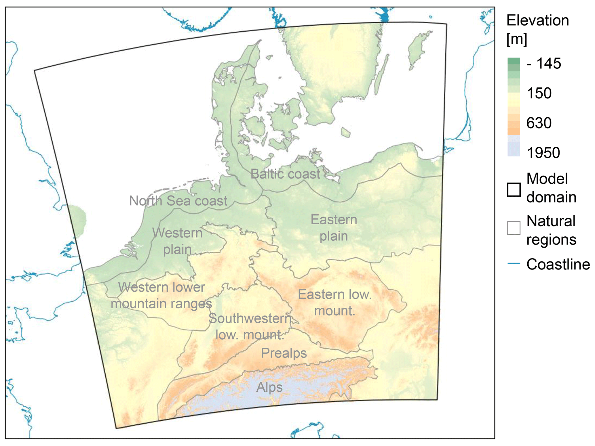
Figure 1 Extent of the CPS model domain. Colors show the elevation (source: EU-DEM, Copernicus Land Monitoring Service, 2016). The natural regions outlined in gray were adapted from Bundesamt für Naturschutz (2017).

For the projection simulations, three 30-year time slices have been selected, covering the years 1971–2000 (historical, CPS-hist) as well as 2031–2060 and 2071–2100 (scenario, CPS-scen). Coupled Model Intercomparison Project Phase 5 (CMIP5) global model data from the Model for Interdisciplinary Research on Climate (MIROC5; Watanabe et al., 2010) have been dynamically downscaled, applying the RCP8.5 scenario. The downscaling has been performed using an intermediate nesting step of 12 km. This intermediate nesting was performed because it is not advised to perform direct downscaling from global models with resolutions of approx. 100 km or coarser to the very high resolution of approx. 3 km.

The CPS evaluation simulation (CPS-eval) covering the 1971–2019 time range is driven by ERA5 (Hersbach et al., 2020) for the years from 1979 to 2019 and by ERA-40 reanalysis data (Uppala et al., 2005) for the years from 1971 to 1978. ERA5 and ERA-40 are reanalysis data that provide comprehensive and coherent information on essential climate variables by assimilating additional various observational data to a model grid. The model system itself remains unchanged throughout the entire time period, resulting in a consistent approach to data assimilation and various parameterizations. For the ERA-40-driven time period, we used a twofold nesting with a middle step at 0.11^∘, whereas a direct downscaling from 30 to 3 km was applied for the ERA5-driven time period. The evaluation simulation driven with reanalysis data serves as a reference for the historical simulation driven by a global climate model. It quantifies how well the historical climate can be reproduced by the historical simulation and how large the differences in specific climate variables are between both simulations. In addition, Rybka et al. (2022) used the evaluation simulation for a comparison with high-resolution observational precipitation data sets to analyze the model performance for extreme precipitation.

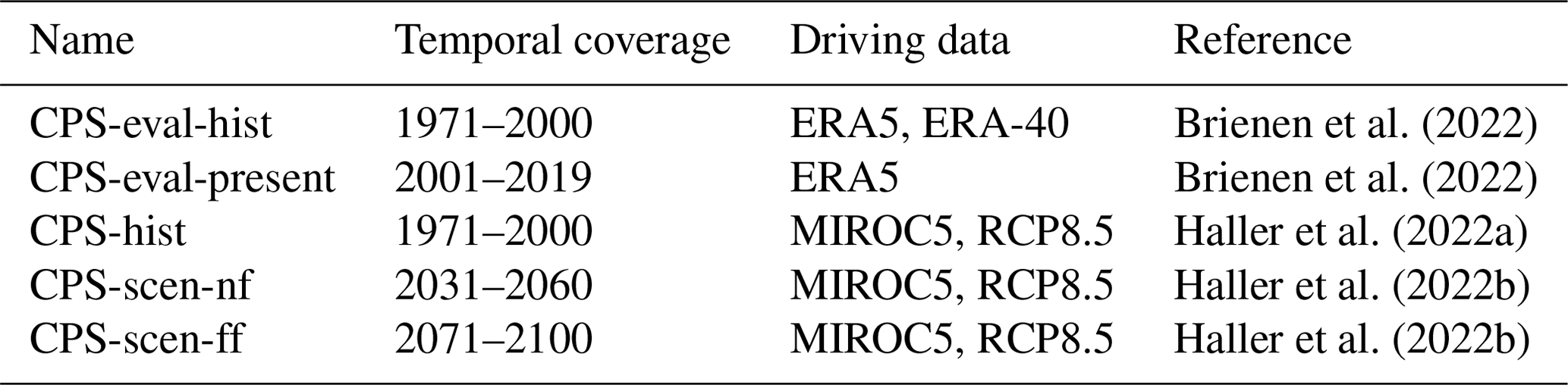
The COSMO-CLM CPS model output consists of hourly data for the most important variables (e.g., temperature, precipitation, humidity and wind). It is available at https://esgf.dwd.de/projects/dwd-cps/ (last access: 10 February 2023) (Brienen et al., 2022; Haller et al., 2022a, b). The overall configuration of our simulation has been taken from a joint contribution of the CLM-Community to a CPS experimental study for central Europe (Coppola et al., 2020). The hourly precipitation data that were further processed for this study were organized in five data sets (Table 1): the projection simulations for the historical period and the near and far future (CPS-hist, CPS-scen-nf and CPS-scen-ff, respectively) as well as the evaluation simulations for the historical period and the present (CPS-eval-hist and CPS-eval-present, respectively).

Table 1 Information on the five data sets that were used for rainfall erosivity calculation.

2.2 Calculation of rainfall erosivity

2.2.1 High-temporal-resolution approach

Following Wischmeier and Smith (1958, 1978) and Wischmeier (1959), the erosivity of an erosive rain event R_e (N h⁻¹) is calculated as the product of maximum 30 min rain intensity I_max30 (mm h⁻¹) and kinetic energy E_kin (kJ m⁻²) of the rain event:

$$\begin{array}{}\text{(1)}& R_{\mathrm{e}}=I_{\max \mathrm{30}}\cdot E_{\mathrm{kin}}.\end{array}$$

An erosive rain event is defined as having a total precipitation (P) of at least 12.7 mm or a maximum 30 min rainfall intensity (I_max30) of at least 12.7 mm h⁻¹ and at least 6 h without any precipitation between two erosive rain events. We used the classical equation by Wischmeier and Smith (1978) to calculate kinetic energy based on high-resolution rainfall data. Transferred to International System of Units (SI) base units, it calculates specific kinetic energy per millimeter rain depth, e_kin,i (in kJ m⁻² mm⁻¹) for every time increment during an erosive rainfall event as follows (Rogler and Schwertmann, 1981):

$$\begin{array}{}\text{(2)}& e_{\mathrm{kin},i}=\left\{\begin{array}{ll}\mathrm{0}& \text{for}I<\mathrm{0.05}\text{mm}{\text{h}}^{-\mathrm{1}}\\ \left(\mathrm{11.89}+\mathrm{8.73}\cdot {\log }_{\mathrm{10}}I\right)\cdot {\mathrm{10}}^{-\mathrm{3}}& \text{for}\mathrm{0.05}\text{mm}{\text{h}}^{-\mathrm{1}}\\ & \le I<\mathrm{76.2}\text{mm}{\text{h}}^{-\mathrm{1}}\\ \mathrm{28.33}\cdot {\mathrm{10}}^{-\mathrm{3}}& \text{for}I\ge \mathrm{76.2}\text{mm}{\text{h}}^{-\mathrm{1}}.\end{array}\right.\end{array}$$

To obtain E_kin for each event, e_kin,i is multiplied by the rain depth of each time step and summed for the entire rain event. Annual rainfall erosivity of a specific year is obtained by summing the R_e of all erosive rain events in that year. The USLE R factor is the long-term average of annual rainfall erosivity. R factors are often given in the unit MJ mm ha⁻¹ h⁻¹ a⁻¹. To convert rainfall erosivity as given here in N h⁻¹ a⁻¹ to MJ mm ha⁻¹ h⁻¹ a⁻¹, it has to be multiplied by a factor of 10.

Here, we calculated annual erosivity as well as long-term average annual erosivity for each one of the 175 545 grid points and for each of the five data sets (CPS-hist, CPS-scen-nf, CPS-scen-ff, CPS-eval-hist and CPS-eval-present). We used the Climate Data Operators (CDO) command line suite (Schulzweida, 2022) and the ncdf4 library (Pierce, 2019) of the R statistical software to extract a time series of 30 years (19 years for CPS-eval-present) for each grid point and each data set and then calculated rainfall erosivity as described above. As the COSMO-CLM model output is available at a temporal resolution of 60 min, three adjustments were made as proposed by Fischer et al. (2018): (i) the rainfall intensity threshold of I_max30 to define an erosive rain event was lowered from 12.7 to 5.8 mm h⁻¹, (ii) I_max30 in Eq. (1) was replaced by a maximum 60 min rainfall erosivity I_max60 and (iii) a temporal scaling factor of 1.9 was applied to the R factor for Germany to account for the reduction in intensity peaks with lower-temporal-resolution data. Here, we did not apply a spatial scaling factor because it is unclear if such a modification is necessary for climate model output.

We further assessed the seasonal distribution of erosivity by calculating the erosion index for each day of the year. The erosion index gives the contribution of each day to annual erosivity (in % d⁻¹). The seasonal distribution of erosivity is important for soil erosion assessments, because of its interactions with seasonal changes in the crop cover. Briefly, high rainfall erosivity in months when vegetation cover is scarce (in central Europe the winter months) is more severe than high rainfall erosivity during the vegetation period (i.e., the summer months). The erosion index was calculated for each of the 175 545 grid points and each day of each year and averaged over all grid points and all 30 years in the three data sets from the projection simulations (CPS-hist, CPS-scen-nf and CPS-scen-ff). The erosion index varies strongly from one day to another and between grid points. Even averaged over all grid point and over 30 years, there still is a high remaining scatter; therefore, a 13 d moving average is used for smoothing of the curves for the three data sets.

2.2.2 Low-temporal-resolution approach

For comparison, we also calculated rainfall erosivity (R) for the past (1971–2000), near future (2031–2060) and far future (2071–2100) from mean annual precipitation (MAP). Therefore, we used the empirical regression equation

$$\begin{array}{}\text{(3)}& R\left[\mathrm{N}{\mathrm{h}}^{-\mathrm{1}}{\mathrm{a}}^{-\mathrm{1}}\right]=\mathrm{0.0788}\cdot \mathrm{MAP}\left[\mathrm{mm}\right]-\mathrm{2.82}\end{array}$$

from the German norm DIN 19708 (DIN-Normenausschuss Wasserwesen, 2017), which was derived from regression analysis of R-factor values calculated based on Eq. (1) and annual precipitation sums for the time period from the 1960s to the 1980s in Germany. We used the median, 15th percentile and 85th percentile of the MAP of a climate model ensemble consisting of 21 members that were run with the RCP8.5 emission scenario. The models are part of the DWD reference ensemble (https://www.dwd.de/ref-ensemble, last access: 20 October 2022). The low-temporal-resolution approach was used here because it allows a representation of the bandwidth of results obtained with a RCM ensemble and, thus, an estimate of model uncertainty, which is not yet possible for CPSs. Nonetheless, the main limitation, i.e., neglect of the effect of increases in heavy rain, of the approach has to be stressed again. This shortcoming is overcome by CPSs and is one of the reasons why the most recent version of DIN 19708 (DIN 19708:2022-08) recommends using Eq. (3) solely for historical observations.

3 Results and discussion

3.1 Past, present and future rainfall erosivity

3.1.1 Rainfall erosivity maps

The average annual rainfall erosivity maps for the five data sets show a consistent spatial pattern (Fig. 2), which is mainly driven by topography. In all data sets, erosivity is lowest in the lowlands of the North European Plain and highest in the Alps. In the past and present, average annual erosivity in the lowlands ranges between approx. 50 and 90 N h⁻¹ a⁻¹. In the Alps, it ranges between 260 and 290 N h⁻¹ a⁻¹, and it ranges between about 90 and 130 N h⁻¹ a⁻¹ in the lower mountain ranges. In the past, the mean of the entire modeling domain is 91 N h⁻¹ a⁻¹ in the evaluation run (CPS-eval-hist) and 96 N h⁻¹ a⁻¹ in the projection run (CPS-hist). It increased considerably in the future (Sect. 3.2). These maps are available on Zenodo (Uber et al., 2023) and can be used as R-factor maps in USLE-based soil erosion modeling.

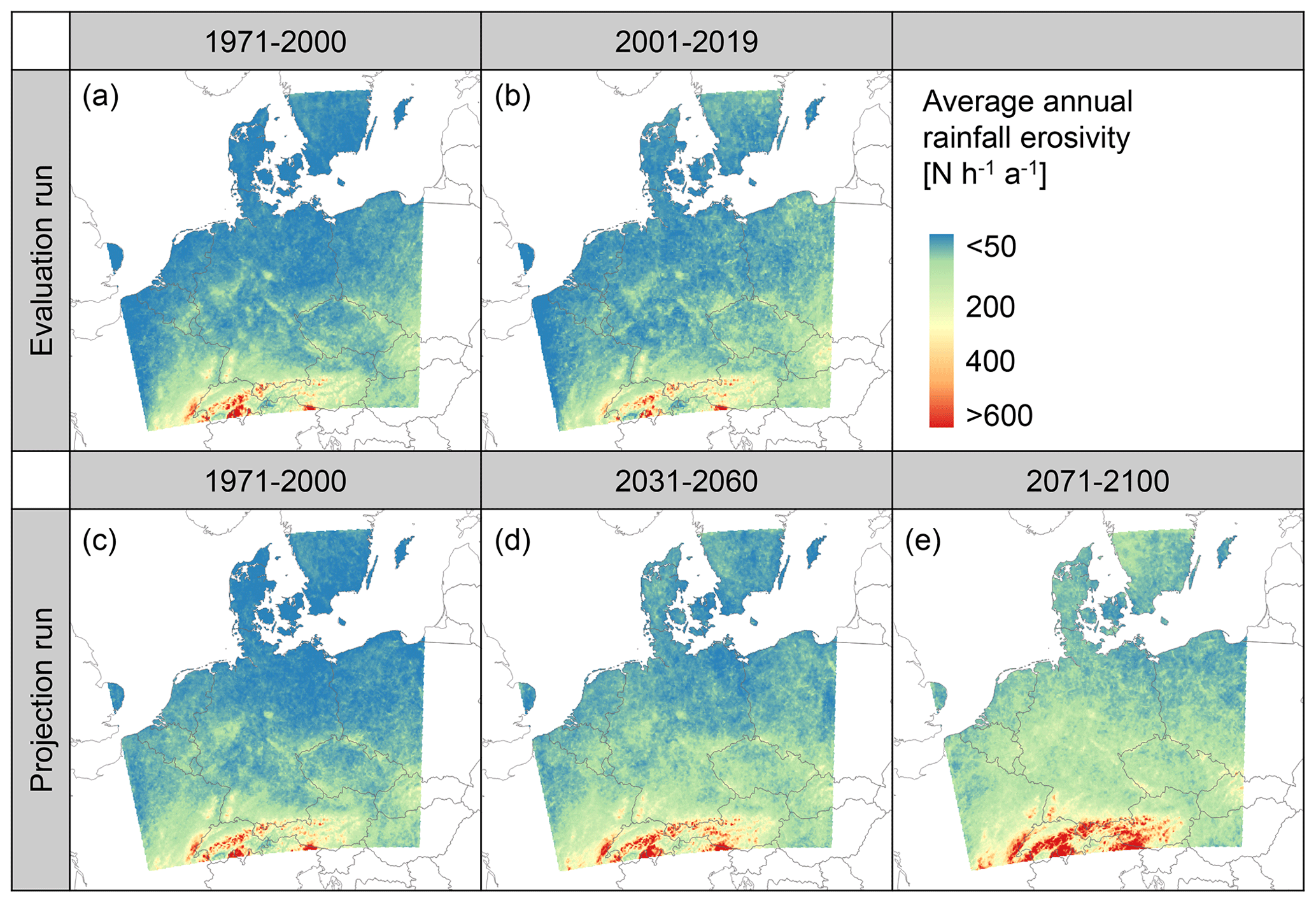
Figure 2 Average annual rainfall erosivity (R factor) in central Europe in the past, present and future derived from the evaluation run (a–b) and the historic and future projection simulations (c–e).

The maps for the past calculated from the evaluation run and the projection run are very similar (Fig. 2a, c). The spatial mean of the difference between the maps is 4.9 N h⁻¹ a⁻¹, and the values for all grid points extracted from the two maps correlate well (R²= 0.91; Fig. S1 in the Supplement).

Beyond erosion modeling, rainfall erosivity can also be regarded as an index of heavy rain that combines rainfall intensity and cumulative precipitation depth. As such, the rainfall erosivity data presented here can also provide valuable information for other hydrological applications dealing with extreme rainfall such as the assessment of (future) risks of flash floods or landslides or identifying zones that are prone to these natural risks (Fiener et al., 2013; Panagos et al., 2015b).

3.1.2 Comparison to other rainfall erosivity maps

Past and present rainfall erosivity can be compared to other available rainfall erosivity maps. Figure 3 shows that rainfall erosivity calculated from the evaluation simulation for 2001–2019 agrees well with the rainfall erosivity map by Auerswald et al. (2019a). The correlation between the values of the raster cells is very good (R²= 0.94) and the slope of the linear regression model is 0.98, i.e., very close to 1. Thus, there is no systematic difference between the two data sets, and the spatial structure corresponds well to that found by Auerswald et al. (2019a). Nonetheless, there are regional differences. Rainfall erosivity in the very north of Germany and in the northwest is underestimated here when compared with Auerswald et al. (2019a), whereas it is overestimated in parts of eastern Germany, the Black Forest and in the Alps (Fig. 3b). The highest values reported here (> 500 N h⁻¹ a⁻¹) are not found by Auerswald et al. (2019a). This might be due to the overestimation of extreme precipitation in COSMO-CLM (Sect. 3.3; Rybka et al., 2022). Compared with the other rainfall erosivity maps for Europe (Panagos et al., 2015b), the Czech Republic (Hanel et al., 2016b) and Austria (Johannsen et al., 2022), our values are, on average, about 2 times higher than those of the other authors. Nonetheless, the correlation is good (0.85–0.96), so the spatial patterns agree well. In general, differences are highest in the mountains and lower in the plains. Here, we did not correct the precipitation data for snow (i.e., no consideration of precipitation on days below 0 ^∘C), in contrast to the methodology of studies such as Johannsen et al. (2022) and Hanel et al. (2016b). This could explain parts of the differences, especially in the mountains. The differences could also be due to the different temporal coverage of the precipitation data used to generate the maps. The temporal coverage of our map (2001–2019) is very similar to that of the map by Auerswald et al. (2019a) (2001–2017) but agrees less with the temporal coverage of the maps of the other authors (1995–2015 for Johannsen et al., 2022; 1989–2003 for Hanel et al., 2016b; and 1970–2017 with a predominance of the last decade for Panagos et al., 2015b). Differences in temporal coverage are especially important given the observed increases in R factors in the last decades (e.g., Hanel et al., 2016a; Auerswald et al., 2019a, b). Furthermore, our methodology is very similar to that of Auerswald et al. (2019a) (e.g., calculation from contiguous data, hourly precipitation data, same temporal scaling factor and same equation used to calculate e_kin,i), whereas it differs from the methodology used by the other authors. The effect of using different equations to calculate e_kin,i was investigated by Hanel et al. (2016b) and Nearing et al. (2017). The former authors found that average rainfall erosivity in the Czech Republic varied strongly between 500 and 760 MJ mm ha⁻¹ h⁻¹ when 14 different equations were used. The USLE equation (which was used here) resulted in the highest values. Nearing et al. (2017) compared rainfall erosivity calculated with USLE, RUSLE (Brown and Foster, 1987, equation) and RUSLE2 and found that, on average, the values obtained with RUSLE and RUSLE2 were 14 % and 3.7 % lower than when USLE was used, respectively. A further important source of uncertainty is the choice of the scaling factors. Here, we used a temporal scaling factor of 1.90 that was established by Fischer et al. (2018) for Germany. This value is remarkably similar to the value of 1.87 established by Yue et al. (2020) for China. Keeping in mind that the temporal scaling factor of 1.56 established by Panagos et al. (2015b) for Europe was used for the conversion of 60 min data to 30 min data and that a second factor (0.80${}^{-\mathrm{1}}=$ 1.25) was established by the same authors for the conversion between 5 and 30 min data, the conversion factor is also similar. The assumption of a constant scaling factor for the entire model domain and the entire simulated time with different types of rain and shifting intensity patterns is certainly a simplification of reality that adds uncertainty. Here, we only used a temporal scaling factor and no spatial scaling factor because the results were in good agreement with those of Auerswald et al. (2019a). It is surprising that no spatial scaling factor was needed here, despite the resolution of 3 km that certainly smoothes sub-grid-scale variability in rainfall intensity and reduces local intensity peaks. Thus, other scaling factors, such as spatial scaling factors or bias correction between measured and simulated precipitation, might be necessary elsewhere, and the temporal scaling factor might have to be adapted to future data with higher intensities of extreme events.

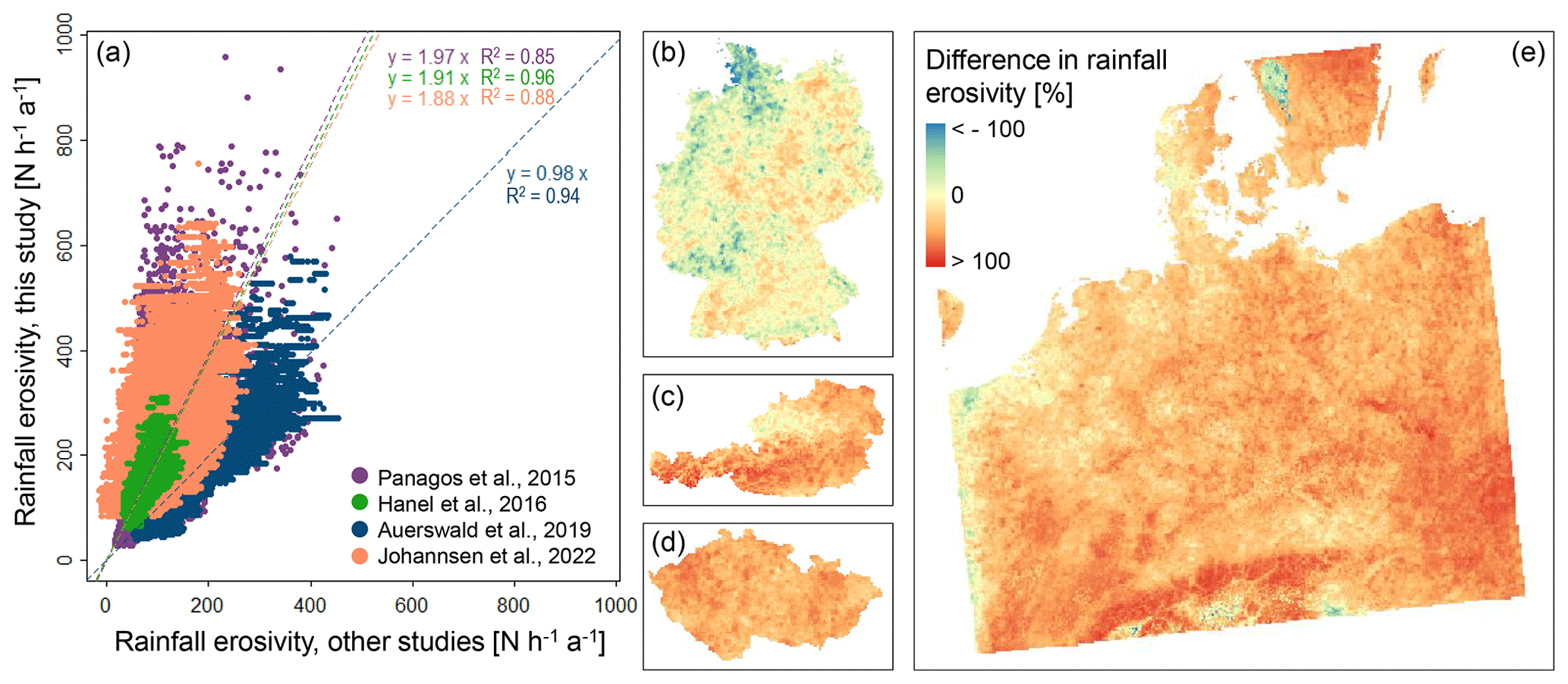
Figure 3 Comparison of the present rainfall erosivity map generated here (evaluation run, data from 2001 to 2019) with maps presented by other authors. In panel (a), each point corresponds to a raster cell; the dashed lines show the linear models fit to the data. Panels (b)–(e) show maps of differences between the map presented here and (b) the map for Germany by Auerswald et al. (2019a) covering the years 2001–2017, (c) the map for Austria by Johannsen et al. (2022) covering the years 1995–2015, (d) the map for the Czech Republic by Hanel et al. (2016b) covering the years 1989–2003 and (e) the map for central Europe by Panagos et al. (2015b) covering the years 1970–2017 with a predominance of the last decade.

In order to quantify the effect of using a different equation to calculate specific kinetic energy from rainfall intensity, we used a subset of our data (about 8 % of the model domain located partly at the coast and partly in the Alps, covering 30 years from 1971 to 2000) to recalculate rainfall erosivity with the RUSLE equation. The USLE-based R factors are, on average, 1.23 times higher than those obtained with the RUSLE equation.

3.1.3 Seasonal distribution of rainfall erosivity

The seasonal distribution of rainfall erosivity shows a clear peak in the summer months (late-May–August; Fig. 4) and minima from November to March. This seasonal pattern is coherent with the results obtained by Johannsen et al. (2022) for Austria, by Auerswald et al. (2019a) for Germany and by Meusburger et al. (2012) for Switzerland. There is a strong variability from one day to another and between subregions of the modeling domain (light gray lines and dashed black line in Fig. 4). This is coherent with the observations made by Auerswald et al. (2019a) and can be explained by the effect of extreme rains that occur during the same day in several pixels (Auerswald et al., 2019a). Thus, single extreme rainfall events influence the mean values, despite the large number of pixels and the long averaging period of 30 years.

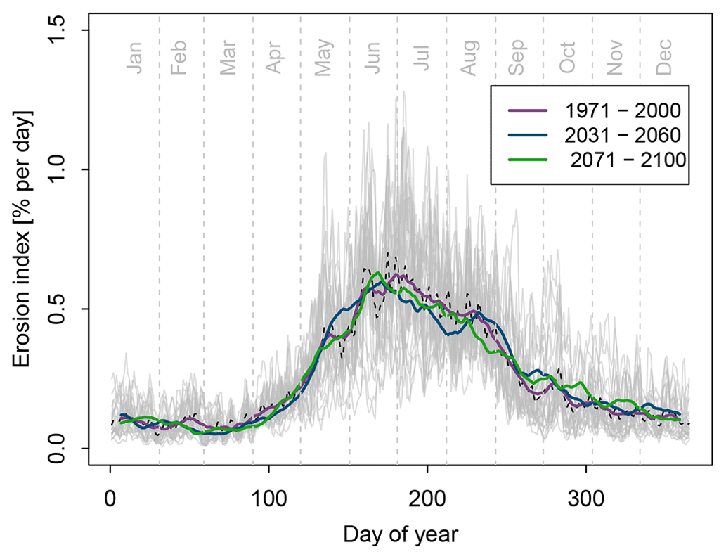
Figure 4 Seasonal distribution of the erosion index. The light gray lines show daily erosion indexes averaged over 30 years in the past (CPS-hist, 1971–2000) and in 25 subregions of the modeling domain. The dashed black line is the average of the entire modeling domain in the past, and the colored lines show the 13 d moving average for each one of the data sets for the past (CPS-hist, 1971–2000), the near future (CPS-scen-nf, 2031–2060) and the far future (CPS-scen-ff, 2071–2100).

The smoothed distribution of the erosion index does not differ considerably between the past, the near future and the far future (Fig. 4). However, a comparison between past and present rainfall erosivity in Germany by Auerswald et al. (2019b) showed that winter erosivity increased considerably. In Switzerland, on the other hand, Meusburger et al. (2012) observed a decreasing trend in rainfall erosivity in February and an increase from May to October. The reasons for the discrepancies between this study, which did not detect significant changes in the seasonal distribution, and the other studies that did observe trends are not clear yet and remain an open question.

3.2 Past and future changes in rainfall erosivity

In the evaluation run, average annual rainfall erosivity increased between the past (1971–2000, mean of 90.5 N h⁻¹ a⁻¹) and the present (2001–2019, mean of 97.8 N h⁻¹ a⁻¹) (Fig. 5). In the projection runs driven by the global climate model, rainfall erosivity increased considerably. This is the case for all statistics (Fig. 5). Mean values increased from 96.3 N h⁻¹ a⁻¹ in the past to 119.3 N h⁻¹ a⁻¹ in the near future and to 149.7 N h⁻¹ a⁻¹ in the far future. Relative changes in average annual rainfall erosivity (in %) between the historical period and the near or far future are highest in the central and northern parts of the modeling domain, i.e., in the basins of the Weser, Ems and Elbe rivers and in the coastal basins in the north (Fig. 6a, e) where rainfall erosivity in the far future can be up to 84 % higher than in the past. Absolute changes, on the other hand, are highest in the basins of the Rhine (28 N h⁻¹ a⁻¹ in the near future and 78 N h⁻¹ a⁻1 in the far future) and the upper Danube (37 and 74 N h⁻¹ a⁻¹, respectively). These are very strong changes. Furthermore, the changes in rainfall erosivity calculated from convection-permitting climate model output are considerably higher than those calculated with the low-resolution approach using mean annual precipitation from model output of conventional RCM ensembles (Fig. 6).

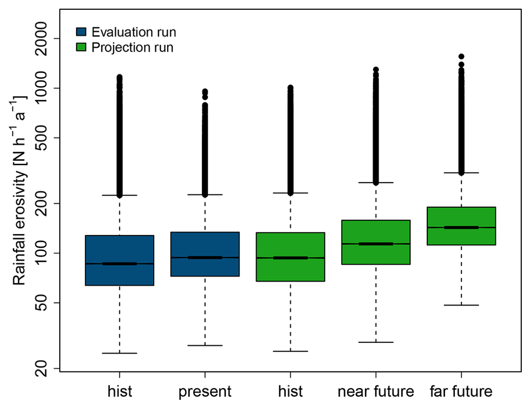
Figure 5 Distribution of the average annual rainfall erosivity (R factor) (N h⁻¹ a⁻¹) in the five data sets.

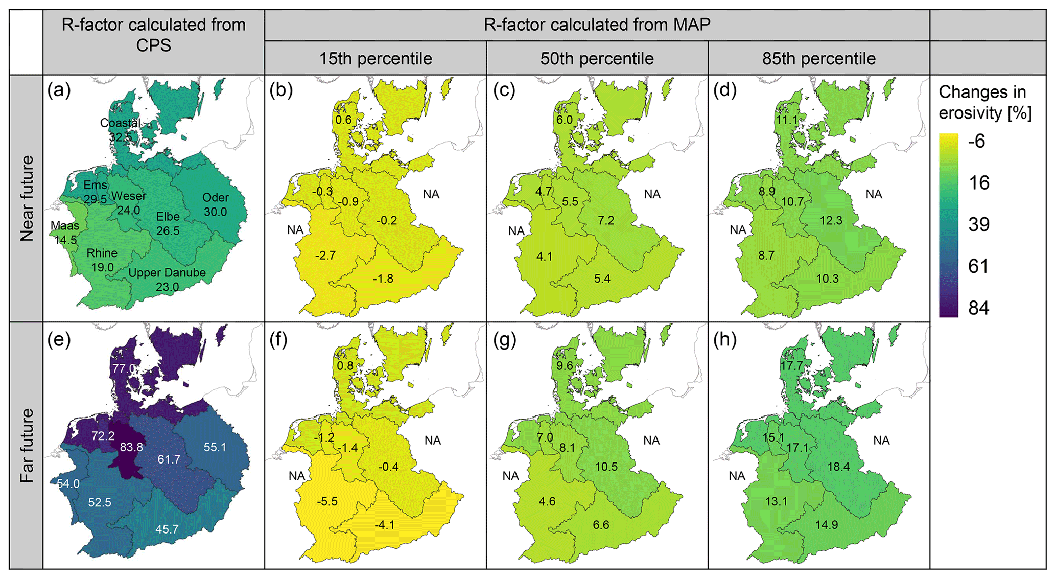
Figure 6 Relative changes in the average annual rainfall erosivity (R factor) in the major central European river basins between the historical period (1971–2000) and the near future (2031–2060, a–d) or the far future (2071–2100, e–h). All values are given as a percentage of the erosivity of the historical period. Panels (a) and (e) show changes in erosivity calculated with the convection-permitting simulations (CPSs); the other panels show changes in erosivity calculated with mean annual precipitation (MAP) obtained from the 15th, 50th and 85th percentiles of 21 regional climate models. All simulations used the RCP8.5 emission scenario.

This is the case not only when future MAP is obtained from the median of the model ensemble but also for the entire plausible bandwidth of models. Figure 6 shows changes in rainfall erosivity estimated with the 15th and the 85th percentiles of the model ensemble. Even though this approach only considers changes in MAP and not changes in rainfall intensity, it allows an estimate of model uncertainty due to the differences between the ensemble members. The results obtained with CPSs are outside of the bandwidth of the model ensemble because they also represent changes in extreme precipitation in addition to changes in MAP.

The finding that the low-resolution approach underestimates future changes in erosivity is in line with the results of Gericke et al. (2019). The regression equation of the German DIN 19708 that was used here (Eq. 3) was established in the early 1990s with climate data from the 1960s to the 1980s. Thus, changes in precipitation characteristics and the fact that it does not consider heavy precipitation raise concerns about using the equation on future data (Gericke et al., 2019). It has to be noted that DIN 19708 explicitly states that, whenever possible, high-frequency precipitation should be used and that Eq. (3) should only be used when only monthly or annual precipitation is available.

Annual rainfall erosivity in all topographic regions of central Europe (coasts, plains, low mountain ranges, Prealps and Alps) shows a strong interannual variability and clear trends (Fig. 7). The high interannual variability observed here is consistent with the findings of other authors, who observed strong interannual variability in rainfall erosivity calculated from measured precipitation data (e.g., Verstraeten et al., 2006; Meusburger et al., 2012; Fiener et al., 2013). The presence of trends supports the conclusions made by other authors: rainfall erosivity maps have to be frequently updated because old rainfall erosivity maps no longer represent current precipitation characteristics (Yin et al., 2017; Auerswald et al., 2019b; Johannsen et al., 2022).

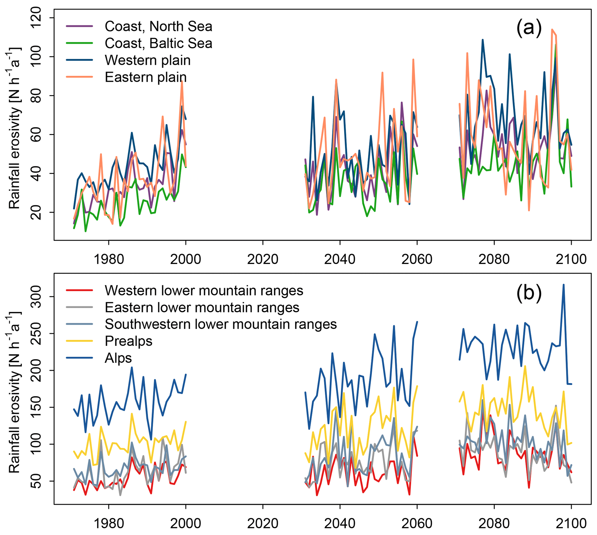
Figure 7 Trends and interannual variability in rainfall erosivity in the natural regions of central Europe for (a) the coast and plains and for (b) the lower mountain ranges, Prealps and Alps. Rainfall erosivity was calculated with precipitation data from the projection run. The natural regions were defined according to Bundesamt für Naturschutz (2017) for Germany and were manually extended to include central Europe based on elevation here. They are outlined in Fig. 1.

While calculating future rainfall erosivity from CPSs offers the advantage of the direct calculation from high-resolution data, it only represents future projections from one model and one emission scenario, which is less robust than using model ensembles. Thus, we compared the past and future changes calculated here to observed and simulated trends in rainfall erosivity in central Europe reported in the literature (Table S1). Both in the past and in the future, the range of reported trends is very large. The values given here agree well with reported values in some cases (e.g., approx. 20 % increase per decade in the Ruhr area of Germany calculated here for the projection run and reported by Fiener et al., 2013, in the 1973–2007 period). In other cases, they are strongly over- or underestimated (Table S1). It also has to be noted that, for the 1971–2000 period, for which we estimated rainfall erosivity from the projection run as well as from the evaluation run, the trends in the two data sets can differ considerably. In most regions, the changes were stronger in the projection run than in the evaluation run.

The high range of trends reported in the literature shows the need to consider model ensembles and to conduct sensitivity analyses to differences in methodology in future research. A comparison with the literature suggests that actual future changes could even be higher than reported here. Such strong changes in rainfall erosivity in the order of > 10 % per decade, as reported by Panagos et al. (2017, 2022), would have important implication for future soil erosion as well as for the occurrence of other natural risks such as landslides and flash floods that are triggered by heavy-rain events.

3.3 Potential and limitations of convection-permitting climate simulations for the calculation of rainfall erosivity

The maps presented here offer a high potential for erosion modeling and climate impact studies. Due to the high resolution of 3 km, they can represent the high spatial variability in rainfall erosivity in a large domain in central Europe. Unlike most other R-factor maps (e.g., Meusburger et al., 2012; Panagos et al., 2015b; Hanel et al., 2016b), our maps do not rely on spatial interpolation and correlation with other spatial covariates such as elevation, latitude, longitude or climate indices.

Because of the high temporal resolution of the underlying precipitation data, we did not have to rely on correlations between R factors calculated at a high resolution and low-resolution rainfall totals such as MAP. Many studies find a good correlation between MAP and R factors, suggesting that MAP is a good covariate to estimate R at locations where no high-resolution precipitation data are available. However, using empirical relations between past MAP and past R factors to derive future R factors is problematic, as it is unlikely that these relations remain stationary in the future (Quine and Van Oost, 2020). These relations are strongly conditioned by the frequency and magnitude of rainfall events that will very likely change in a warmer climate. In several regions in Europe, such as the Mediterranean (Tramblay et al., 2012; Blanchet et al., 2018) and the Carpathian Basin (Bartholy and Pongrácz, 2007), MAP is decreasing while extreme precipitation is increasing. This leads to an underestimation of future R factors that are derived from MAP alone. In central Europe, both MAP and extreme precipitation are expected to increase (Jacob et al., 2014; Brienen et al., 2020); thus, future R factors derived from MAP are also underestimated, although less severely than in the abovementioned regions. Because changes in MAP as well as in extreme precipitation are well represented in CPSs, they offer a valuable data source for the calculation of future rainfall erosivity.

Even when the same temporal resolution (3 h) of simulated precipitation data was compared, Chapman et al. (2021) found that rainfall erosivity was considerably higher and observed storm characteristics agreed better with simulated ones when a convection-permitting model was used instead of a conventional convection-parameterized one.

On the other hand, the maps presented here also have limitations. Here, we calculated rainfall erosivity from precipitation data and did not consider whether precipitation falls as rain, snow or hail; therefore, the high erosivity of hail is underestimated, while erosivity in zones where considerable amounts of precipitation fall as snow (i.e., mainly the Alps) is overestimated. As rainfall erosivity in central Europe is highest in the summer months, we assume that the impact of snow is small and can be neglected. For the Alps, this is not the case; thus, the very high values calculated in this region are too high.

As our maps are calculated from model output and not from precipitation measurements, the uncertainties in the model are propagated to the rainfall erosivity maps. The precipitation data were quality controlled and compared to radar- and station-based precipitation data from the past but not bias corrected. The data showed a good agreement for extreme rainfall intensities for durations of more than 12 h but an overestimation for hourly extreme precipitation intensities (Rybka et al., 2022). This leads to an overestimation of the rainfall erosivity presented here that has to be kept in mind. Thus, it is important to compare the R factors calculated here to the ones calculated from measured rainfall data.

Concerning the future projections, it has to be noted that current climate models struggle with estimates of future precipitation, and biases are much larger than those for future temperatures (e.g., Slingo et al., 2022). Ensembles of global and regional climate models show a high range of future trends in precipitation that cannot be represented by a single model. Other studies estimated future R factors from ensembles of global or regional climate models such as the CMIP5 model ensemble, the model ensemble from the European part of the Coordinated Downscaling Experiment (EURO-CORDEX) or the DWD reference ensemble (Gericke et al., 2019; Panagos et al., 2022; Uber et al., 2022). In this way, the high range of projections can be represented and the uncertainty due to the choice of climate model and emission scenario can be assessed. Currently, such evaluations of variability between climate models are not possible for convection-permitting climate models, as no model ensembles of multi-decadal simulations over large domains are available. In COSMO-CLM, so far, only simulations driven with RCP8.5 have been performed; therefore, no data driven with the other emission scenarios are available. However, there are promising flagship studies such as the flagship pilot studies (FPS) from the CORDEX initiative, in which a first multi-model convection-permitting ensemble for the Alps and the Mediterranean is presented (Coppola et al., 2020). Furthermore, the latest generation of Coupled Model Intercomparison Project Phase 6 (CMIP6) global climate models suggests that the decrease in summer precipitation in central Europe might be stronger than previously estimated by the CMIP5 model ensemble (Palmer et al., 2021; Ritzhaupt and Maraun, 2023), but these global models are only being downscaled by regional models now. Thus, the soil erosion modeling community should closely follow the coming advances in convection-permitting modeling to take advantage of new climate simulations for climate impact studies.

4 Conclusions

We calculated rainfall erosivity (quantified as the USLE R factor) in central Europe in the past (1971–2000), present (2001–2019), near future (2031–2060) and far future (2071–2100) from convection-permitting simulation (CPS) output. From this work, we draw three main conclusions:

• Thanks to the high spatiotemporal resolution of CPSs (in this case 3 km and 1 h), R factors can be calculated directly without having to rely on spatial interpolation and regression with aggregated precipitation sums such as mean annual precipitation (MAP). Thus, CPSs offer a high potential for the calculation of future R factors for climate impact studies on soil erosion. For the present, the R-factor map presented here is very similar to the map by Auerswald et al. (2019a) that was calculated from radar-derived precipitation data.

• In the river basins in central Europe, assuming the RCP8.5 emission scenario, changes in rainfall erosivity between the past and the near future can be as high as 33 %, whereas they can be up to 84 % higher in the far future. These rates of change are much higher than estimated previously using regression with MAP. This is due to the fact that the intensification of extreme precipitation is not represented by changes in MAP. This indicates that correlations between R factors and MAP that were developed in the past are not necessarily valid in the future.

• A major limitation of CPSs is their high computational demand. Thus, model domains are usually limited to much smaller spatial extents than those covered by global or regional climate models or the simulated time periods are limited to short time periods. The simulations in COSMO-CLM cover a long time period (109 years in total) and a comparably large modeling domain of approx. 1.6×10⁶ km² on land. However, to date, no ensembles of CPSs are available at the regional scale and for long time periods. Thus, in contrast to global or regional climate models, the uncertainty in future R factors due to the choice of climate models cannot yet be estimated by using a bandwidth of model ensembles. Promising advances in the CPS community – including flagship studies on CPS model ensembles – suggest that, in the future, more CPSs will be available for climate impact studies on soil erosion.