Employing the generalized Pareto distribution to analyze extreme rainfall events on consecutive rainy days in Thailand's Chi watershed: implications for flood management

Extreme rainfall events in the Chi watershed of northeastern Thailand have significant implications for the safe and economic design of engineered structures and effective reservoir management. This study investigates the characteristics of extreme rainfall events in the watershed and their implications for flood risk management. We apply extreme value theory to historical maximum cumulative rainfall data for consecutive rainy days from 1984 to 2022. The generalized Pareto distribution (GPD) was used to model the extreme rainfall data, with the parameters estimated using maximum likelihood estimation (MLE) and linear moment estimation (L-ME) methods based on specific conditions. The goodness-of-fit tests confirm the suitability of the GPD for the data, with p values exceeding 0.05. Our findings reveal that certain regions, notably Udon Thani, Chaiyaphum, Maha Sarakham, Tha Phra Agromet., Roi Et, and Sisaket provinces, show the highest return levels for consecutive 2 d (CONS-2) and 3 d (CONS-3) rainfall. These results underscore the heightened risk of flash flooding in these regions, even with short periods of continuous rainfall. Based on our findings, we developed 2D return level maps using the Q-geographic information system (Q-GIS) program, providing a visual tool to assist with flood risk management. The study offers valuable insights for designing effective flood management strategies and highlights the need for considering extreme rainfall events in water management and planning. Future research could extend our findings through spatial correlation analysis and the use of copula functions. Overall, this study emphasizes the importance of preparing for extreme rainfall events, particularly in the era of climate change, to mitigate potential flood-related damage.

1 Introduction

The distribution of rainfall and atmospheric fluctuations are directly impacted by changes in climate, which have significant implications for water resource management and hydrology. The northeastern region of Thailand is particularly susceptible to frequent flooding, which is often caused by a combination of local conditions, natural variations, and human actions. Unfortunately, this issue shows no signs of abating, and it continues to escalate in severity. In the northeastern region of Thailand, there is an agricultural area of over 63×10⁶ rai (1 rai = 1600 m²). However, a significant proportion of this area continues to face challenges such as water scarcity, drought, and occasional natural disasters during heavy rainy seasons.

Over the past three decades, water shortages have affected 57 provinces (or 75 % of the country), 525 districts (or 60 % of the total districts), 3321 sub-districts (or 46 % of the total), and 24 900 villages (or 33 % of the total villages) in Thailand, causing extensive damage. On average, 9.71 million people suffer from drought annually, representing about 15 % of the total population. Additionally, an average of 2.571 million rai of farmland is damaged each year, leading to an average loss of 661 head of livestock. The total cost of damage amounts to THB 656.62 million (or USD 17.57 million) per year. Moreover, the northeastern region has witnessed seven major floods in the years 1983, 1995, 1996, 2002, 2006, 2010, and 2011. These events resulted in substantial harm to both human life and property, posing challenges in accurately evaluating their impact and the overall cost of the incurred damage (Gale and Saunders, 2013; Singkran, 2017; Meteorological, 2021). Gale and Saunders (2013) identified the causes of the major floods that occurred in Thailand in 2011 and presented forecasts for future flooding. Their research indicates that unless flood defenses and management practices are improved, there is a high likelihood of more flooding occurring within the next two to three decades.

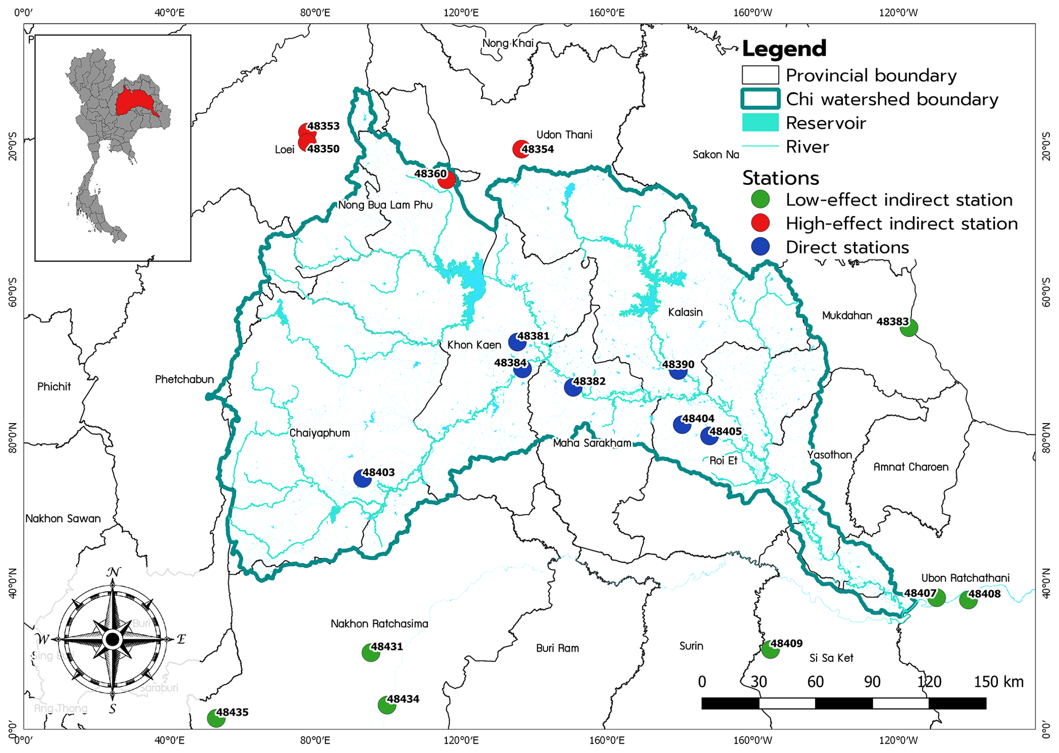
Figure 1 Location of all 18 meteorological stations along the Chi watershed in the northeastern region of Thailand.

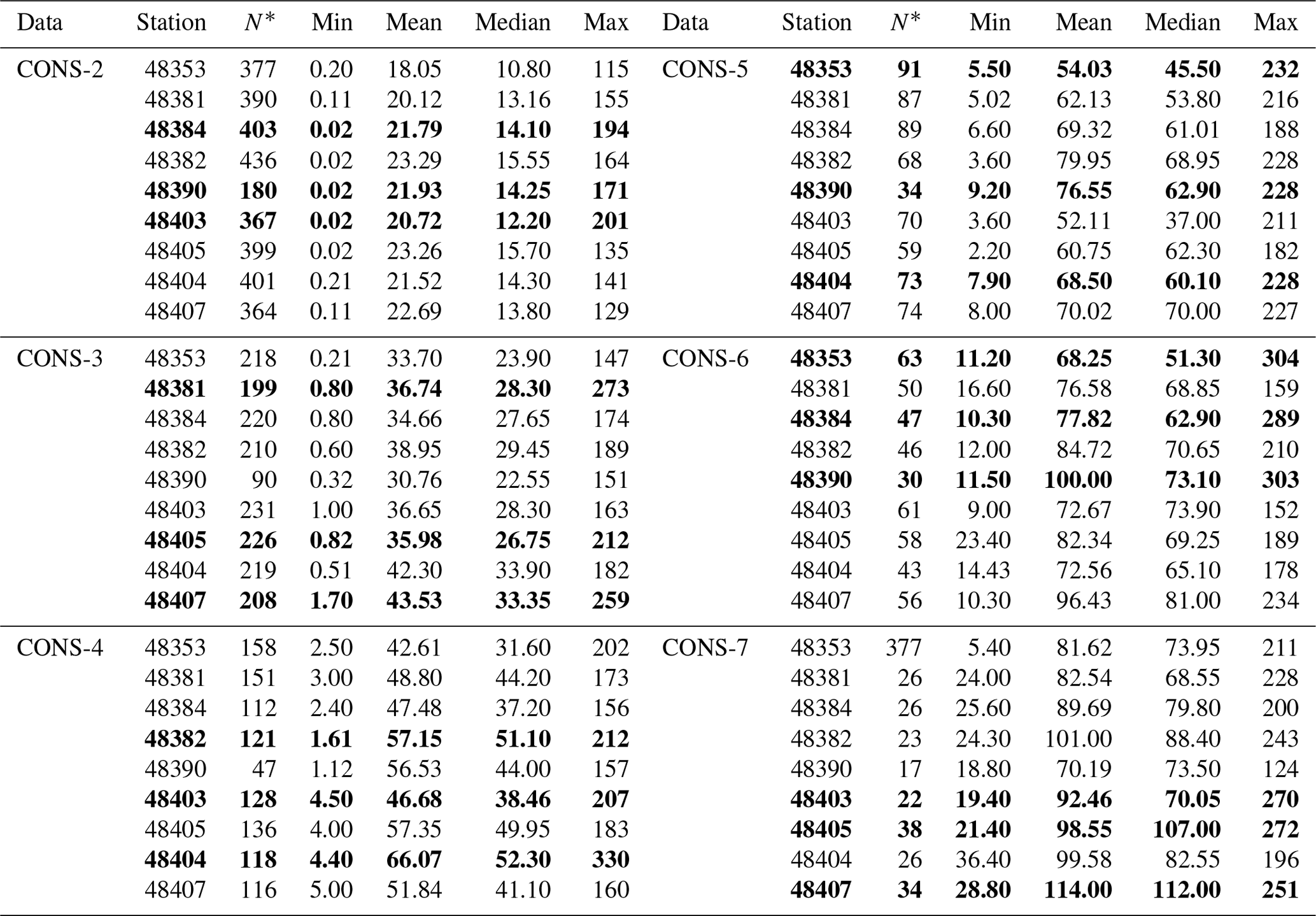
Table 1 Descriptive statistics of the maximum cumulative rainfall on consecutive rainy days for 2, 3, 4, 5, 6, and 7 d are provided for selected stations in the northeastern region of Thailand. N^* represents the number of consecutive rainy days (unit: mm). The top three maximum rainfall values are in bold.

According to the Thai Meteorological Department's report in 2006 (Meteorological, 2021), flood conditions in the Chi watershed occur infrequently during each year. Various studies have also indicated that the area is prone to frequent flooding (Kunitiyawichai et al., 2011; Arunyanart et al., 2017). Flooding in the Chi watershed takes on many different forms, including but not limited to overflowing riverbanks in provinces such as Chaiyaphum, Khon Kaen, and Roi Et; wild water flows in Chaiyaphum, Khon Kaen, and Roi Et; and mudslides in Kalasin and Chaiyaphum provinces. The watershed has also experienced severe flooding in various areas, such as Roi Et, Kalasin, and Khon Kaen Provinces. The Chi watershed is susceptible to flooding due to several factors. First, heavy rainfall resulting from the influence of the southwest and northwest monsoons and depressions from the South China Sea often occurs in the watershed area. Second, the upstream area of the watershed, where the Chi River originates, is characterized by mountainous terrain with steep slopes and has experienced significant deforestation. Third, the lower part of the watershed, particularly in Roi Et and Ubon Ratchathani provinces, is a plain where multiple rivers converge and is the point where the Chi River meets the Mun River before flowing into the Mekong River. This creates drainage issues for the watershed area. Fourth, water management in large reservoirs poses a challenge during the rainy season, as some years require significant amounts of water to be drained due to the high levels of annual rainfall and water discharge from nearby reservoirs (Meteorological, 2021). Given these challenges, effective water management during the flooding and drought seasons is critical. Numerous studies have applied mathematical and statistical theories to address these issues, such as those conducted by Bhakar et al. (2006), Noymanee and Theeramunkong (2019), Suksawang (2012), Hung et al. (2009), and Dutta et al. (2003).

It is well known that floods occur on average every several years, as supported by numerous studies. In this context, Coles (2001) introduced the concept of extreme value theory, which focuses on studying the maximum and minimum occurrences in a data set. These extreme values are typically located at the tail of the distribution and are often disregarded in analysis or modeling due to their perceived complexity and low number. However, extreme value theory provides a framework to better understand and model such events. Extreme analysis is a method employed to assess the severity of natural phenomena, encompassing factors such as maximum–minimum rainfall, temperature extremes, maximum–minimum wind speeds, and more. In their studies, Busababodhin and Kaewmun (2015), Pangaluru et al. (2018), and Wang and Xuan (2020) developed an extreme value model to analyze the probability of extreme events using data from Thailand. They also explored methods for selecting the most suitable extreme value model and determining return periods and return levels. Bhakar et al. (2006) studied the analysis of the frequency of 1 d maximum rainfall and 2–5 d consecutive maximum rainfall at Banswara district in southern Rajasthan of India. Three distributions, i.e., the normal, log-normal, and Gumbel distributions, were used in the analysis for this data and compared with the chi-square value, and the results showed that the Gumbel distribution was the best fit for the region and it was taken for the return level associated with return periods varying from 2 to 100 years. Several studies have investigated the frequency of maximum consecutive days of rainfall and they support the use of extreme value distribution. These studies employed maximum likelihood estimation (MLE) and verified model suitability using tests such as the Kolmogorov–Smirnov (K–S) test and Anderson-Darling (AD) test. Examples of these studies include Kwaku and Duke (2007), Patel et al. (2011), Manikandan and Kumar (2015), and Sabarish et al. (2017).

The current study aimed to fill the research gap by examining the consecutive days of maximum rainfall data for Thailand. This data set was chosen due to the frequent occurrence of flooding caused by continuous heavy rainfall. To the best of our knowledge, no previous studies have been conducted on this specific type of data in Thailand. In this study, we aimed to identify critical areas along the Chi watershed and evaluate their severity for use in planning, resolving flooding, and pre-evaluating damage. To achieve this, we applied the non-stationary (NS) generalized Pareto distribution (NS-GPD) models on the maximum cumulative rainfall data observed for consecutive rainy days (CONS) of 2, 3, 4, 5, 6, and 7 d at 18 stations along the Chi watershed in the northeastern region of Thailand. Section 2 provides an overview of the data and climatology of the Chi watershed in Thailand. Section 3 describes the materials and methods used in the study, including the NS GPD modeling, which considered five models. In Sect. 4, the results of the study are presented, including isopluvial maps of the return levels and their changes over time, which were predicted from the best model. Discussion is provided in Sect. 5, followed by a conclusion in Sect. 6. Technical specifics, tables, and figures are included in the Supplement.

2 Data

In this study, we analyzed the maximum cumulative rainfall on CONS data for 2, 3, 4, 5, 6, and 7 d observed by the Thai Meteorological Department (TMD) (Meteorological, 2021) from 1984 to 2022. The rainfall data ranged from 115.0 to 330.0 mm, with an average range of 17.7–114.44 mm for all stations. Descriptive statistics for the maximum cumulative rainfall on CONS for 2, 3, 4, 5, 6, and 7 d are presented in Table 1 for selected stations. N^* is the number of consecutive rainfalls between 1984 and 2022. We used the maximum cumulative rainfall for CONS to select the number of consecutive days for analysis as in Eq. (1):

$$\begin{array}{}\text{(1)}& \mathrm{CONS}-\mathrm{n}=\sum _{i=\mathrm{1}}^n\left(X_i\right),\end{array}$$

where $X_i>\mathrm{0};X_i$ is rainfall on CONS, such as in the case n=2 and then $\mathrm{CONS}-\mathrm{2}=X_{\mathrm{1}}+X_{\mathrm{2}}$ when X₁,X₂ is rainfall on 1 and 2 consecutive days, respectively. Figure 3 displays the density curves for cumulative rainfall on consecutive days, indicating that all stations were positively skewed and had heavy tails. Further details are provided in the Supplement.

Figure 1 displays the locations of the 18 meteorological stations situated along the Chi watershed in the northeastern region of Thailand, covering 12 provinces. The detailed latitude and longitude of these stations are provided in Table S1 in the Supplement. The Chi watershed falls within the tropics, between latitudes 13^∘00^′–18^∘00^′ and longitudes 101^∘00^′–105^∘00^′.

Table 1 presents descriptive statistics of maximum cumulative rainfall on CONS for periods of 2, 3, 4, 5, 6, and 7 d. The results indicate that the stations Chaiyaphum (48403), Khon Kaen (48381), Roi Et Agromet. (48404), Kalasin (48390), Kalasin (48390), and Roi Et (48405) recorded the highest maximum cumulative rainfall for CONS-2, CONS-3, CONS-4, CONS-5, CONS-6, and CONS-7, respectively. The range of maximum CONS values for 2, 3, 4, 5, 6, and 7 d was between 115 and 330 mm, while the average of CONS for the same durations ranged between 17.7 and 114.44 mm.

Table 2 provides a comparison of Mann–Kendall (MK) test results for CONS data for periods of 2, 3, 4, 5, 6, and 7 d at some selected stations. Out of 18 stations, 9 stations (i.e., 50 % of the total stations) showed a trend in the CONS-2 to CONS-3 data, except for CONS-7. This trend is more evident in Fig. 2, which displays the trends in the CONS-2 and CONS-3 data for the Chaiyaphum station. Consequently, the functional form of parameters for time dependent NS generalized Pareto models was included. Table 3 provides details of the five functional models employed for CONS rainy days.

Table 2 Comparison of the Mann–Kendall test for consecutive rainy days of 2, 3, 4, 5, 6, and 7 d at each station. Mann–Kendall test: ^* p<0.1, ${}^{**}$ p<0.05.

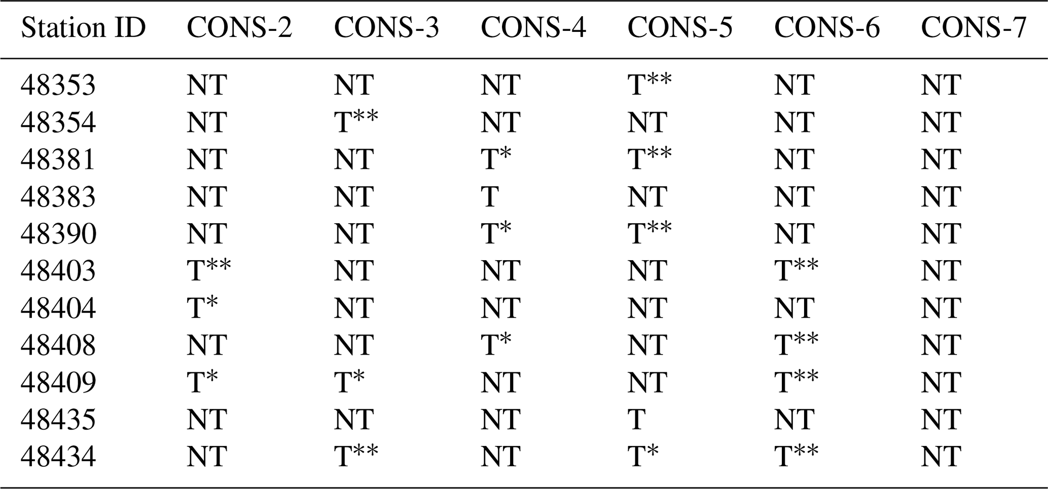
Note: “NT” represents “no trend” in the data and “T” represents the presence of a trend in the data.

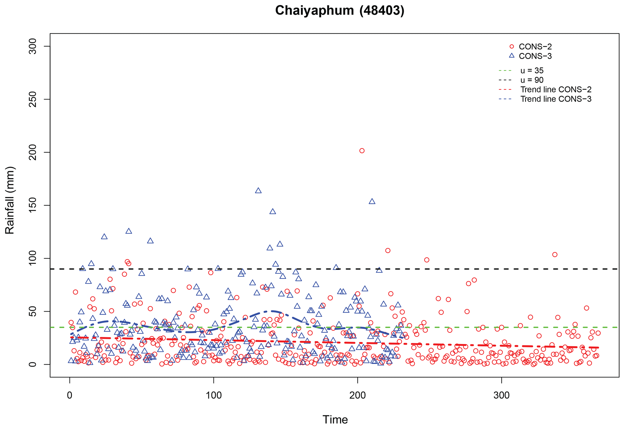
Figure 2 Scatter and line plots showing the trends for CONS-2 and CONS-3 (unit: mm) at the Chaiyaphum meteorological station in the Chi watershed, northeastern Thailand.

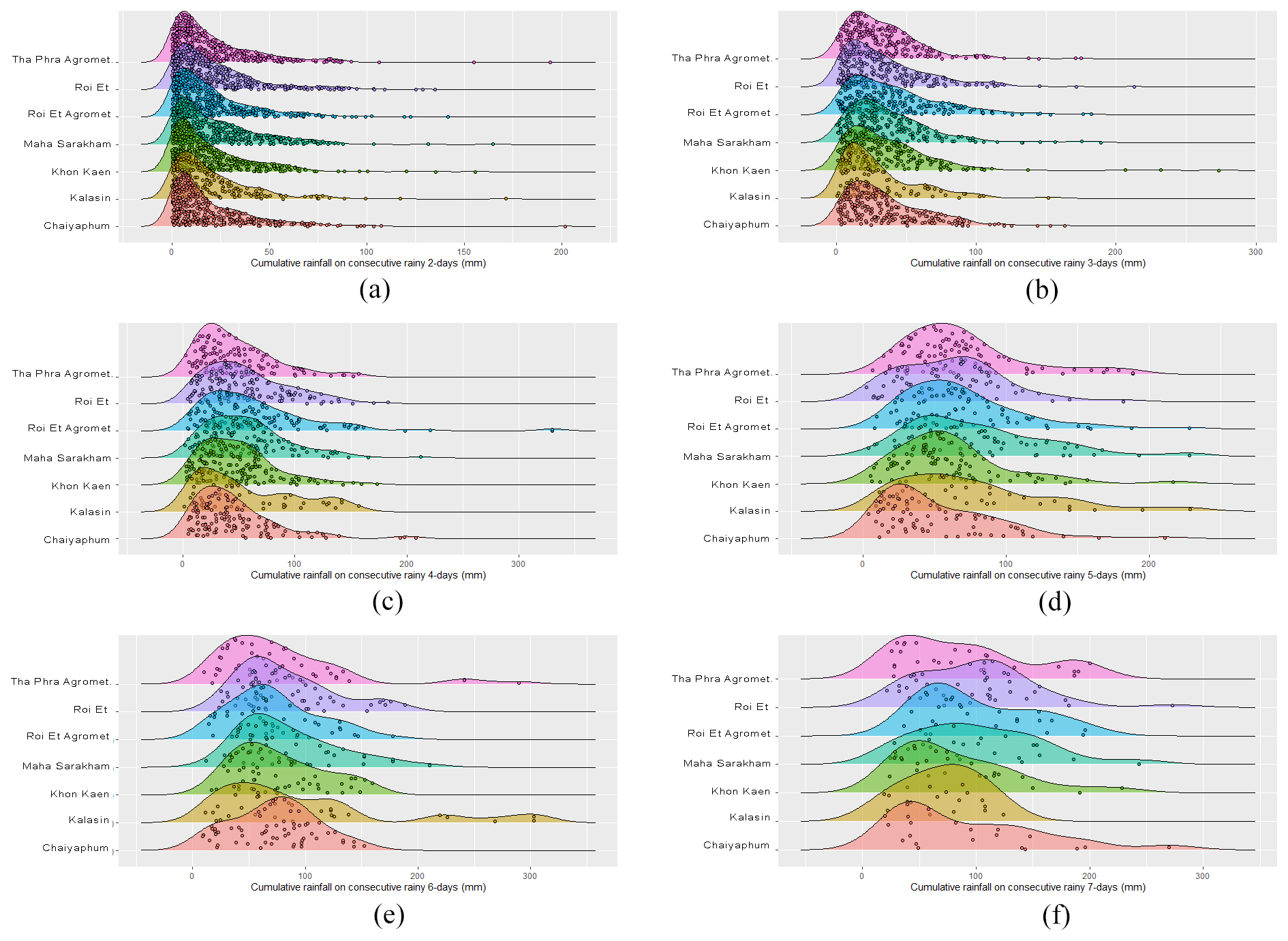
Figure 3 Panels (a)–(f) show ridge line plots for cumulative rainfall on consecutive rainy days (unit: mm) for seven stations including Khon Kaen, Tha Phra Agromet., Maha Sarakham, Kalasin, Chaiyaphum, Roi Et, and Roi Et Agromet. in the Chi watershed, northeastern Thailand.

3 Materials and methods

3.1 Time dependent models for GPD

The block maxima method is limited for analyzing maximum rainfall data each year. Hence, the peak-over-threshold (POT) method or GPD is commonly employed for this purpose (Coles, 2001). The POT method involves selecting observations above a specified threshold value (u) from the data variable X, and expressing the exceedances of X over u as $Y=X-u$. The GPD function is then defined as in Eq. (2):

$$\begin{array}{}\text{(2)}& H\left(y\right)=\mathrm{1}-{\left(\mathrm{1}+{\displaystyle \frac{\mathit{\xi }y}{\stackrel{\mathrm{̃}}{\mathit{\sigma }}}}\right)}^{-\mathrm{1}/\mathit{\xi }},\end{array}$$

defined on y>0, where $\stackrel{\mathrm{̃}}{\mathit{\sigma }}=\mathit{\sigma }+\mathit{\xi }(u-\mathit{\mu })$ is the scale parameter and $-\mathrm{\infty }<\mathit{\xi }<\mathrm{\infty }$ is the shape parameter. In the special case ξ=0 , leading to

$$\begin{array}{}\text{(3)}& H\left(y\right)=\mathrm{1}-\exp (-{\displaystyle \frac{y}{\stackrel{\mathrm{̃}}{\mathit{\sigma }}}}),y>\mathrm{0}.\end{array}$$

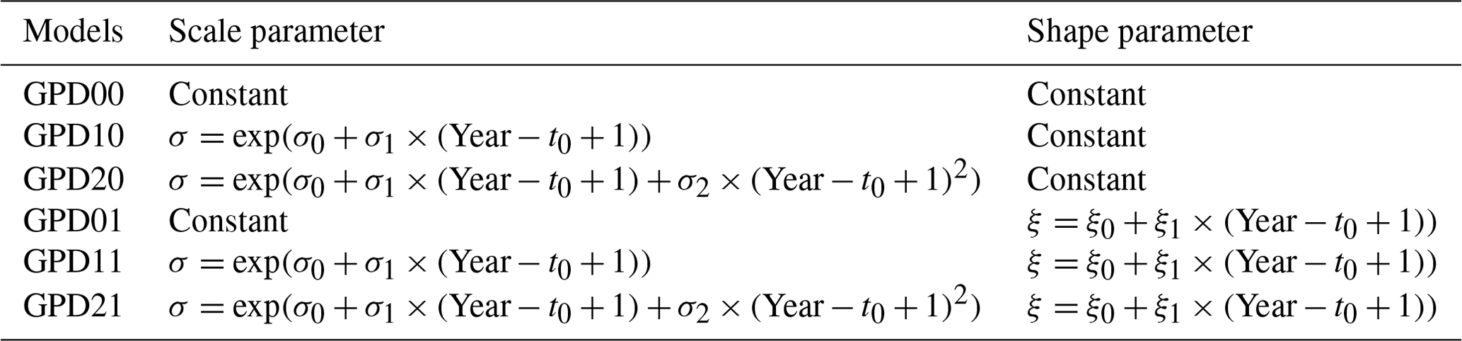
Table 3 Functional form of parameters for time dependent non-stationary extreme value models, represented by GPDab where a represents the scale parameter (σ) and b represents the shape parameter (ξ). The stationary model is represented by GPD00.

The GPD can take on one of three forms depending on the sign of the shape parameter, ξ. Specifically, when ξ>0, the distribution has no upper limit, while ξ<0 indicates an upper bounded distribution and ξ=0 represents an unbounded exponential distribution (Senapeng and Busababodhin, 2017). This notation for the shape parameter is commonly used in statistical literature (see more details in Hosking, 1990; Coles, 2001).

Grouping extreme values based on their independence can be achieved by clustering the values that exceed a certain threshold, which makes the GPD a suitable method for analysis (Coles, 2001). As a result, this method was selected to model the maximum cumulative rainfall on consecutive days. Additionally, the five NS-GPD models considered in this study are presented in Table 3. These models are very important in predicting the behavior of extreme precipitation. Stationary assumptions can lead to inaccurate results when the underlying conditions are changing over time. Therefore, the use of NS models is crucial for accurately capturing the time-varying nature of extreme precipitation, especially in the context of climate change. Consequently, the application of NS models enables a more robust understanding of extreme precipitation patterns and can support informed decision-making for engineering structures and reservoir management in the Chi watershed of Thailand.

3.2 Mann–Kendall test of trend

We considered the Mann–Kendall (MK) test of trend, to compare with the NS-GPD model. The MK test is commonly used to detect monotonic trends in time-series data. In the MK test, the null hypothesis is H₀: no monotone trend in hydro logic series X_t versus the alternative hypothesis which is H₁: monotonic trend in X_t without specification of the sign of the trend. This hypothesis test is two-tailed, so we reject H₀ with α level if $\left|Z\right|>z_{\mathit{\alpha }/\mathrm{2}}$, where Z is a normalized MK test statistic calculated from data (Naghettini, 2017) , and $z_{\mathit{\alpha }/\mathrm{2}}$ is $\mathrm{100}\times (\mathrm{1}-z_{\mathit{\alpha }/\mathrm{2})}$ percentile of the standard normal distribution (Wilks, 2011). An R package “trend” (Pohlert et al., 2016) was used to execute the MK test (Prahadchai et al., 2022).

3.3 Threshold selection method

The selection of an appropriate threshold is a crucial factor in statistical inference of rare events. This study compares three different threshold selection methods and their effectiveness. The first approach involves selecting the threshold based on meteorological conditions, where rainfall greater than 35 mm is considered indicative of heavy rainfall. The second approach uses the 90th percentile of the rainfall data set as the threshold. The third approach involves using the mean residual life (MRL) plot to select a threshold for the GPD or point process models. These approaches are analyzed theoretically and compared with existing procedures through an extensive simulation study, and are then applied to a data set of CONS, where the underlying extreme value index is assumed to vary over time.

3.4 Parameter estimation and model choice

The parameters in the GPD are commonly estimated using either the MLE (Coles, 2001) or the L-ME method (Hosking, 1990). In the present study, the latter method was employed due to its higher efficiency in small samples compared with the MLE method (Naghettini, 2017; Papukdee et al., 2022). Specifically, the “eva” (Bader and Yan, 2016), “extRemes” (Gilleland and Gilleland, 2016), “ismev” (Stephenson, 2011), and “lmom” (Hosking, 2009) packages in R were utilized for this purpose (Hosking, 2022).

Assuming observations $(X_{\mathrm{1}},X_{\mathrm{2}},\mathrm{\dots },X_n)$ follow the GPD, the negative log-likelihood function is

$$\begin{array}{}\text{(4)}& \mathrm{\ell }(\mathit{\sigma },\mathit{\xi })=-k\log \mathit{\sigma }-\left(\mathrm{1}+{\displaystyle \frac{\mathrm{1}}{\mathit{\xi }}}\right)\sum _{i=\mathrm{1}}^k\log \left(\mathrm{1}+\mathit{\xi }{\displaystyle \frac{y_i}{\mathit{\sigma }}}\right),\end{array}$$

provided $\left(\mathrm{1}+\mathit{\xi }(y_i/\mathit{\sigma })\right)>\mathrm{0}$ for $i=\mathrm{1},\mathrm{2},..,k;$ otherwise, $\mathrm{\ell }(\mathit{\sigma },\mathit{\xi })=-\mathrm{\infty }$. In the case ξ=0 the log-likelihood is obtained from Eq. (3) as

$$\begin{array}{}\text{(5)}& \mathrm{\ell }(\mathit{\sigma },\mathit{\xi })=-k\log \mathit{\sigma }-{\displaystyle \frac{\mathrm{1}}{\mathit{\sigma }}}\sum _{i=\mathrm{1}}^k{y}_i.\end{array}$$

The L-ME is widely used in analyzing skewed data, such as extreme rainfall and flood frequency. Although the details of the L-ME are not discussed here, we note that it is considered a standard method in such analyses. To calculate the L-ME of the GPD, we utilize the R package “lmom” developed by (Hosking, 2009). However, one potential disadvantage of the L-ME is that Newton–Raphson type algorithms used to solve systems of L-moments equations may sometimes fail to converge (Dupuis and Winchester, 2001; Papukdee et al., 2022).

3.5 Model diagnostics and goodness-of-fit test

The performance of the marginal probability was evaluated by conducting goodness-of-fit statistical tests. In this study, two tests – the Kolmogorov–Smirnov and Anderson-Darling tests – were used for this purpose. The K–S test is preferred as it does not make any assumptions about the distribution of data (Glen et al., 2001). This method involves comparing the maximum gap between the experimental cumulative distribution function and the theoretical cumulative distribution function. The K–S test $\left(D_{n,n^{\mathit{\tau }}}\right)$ is used to determine whether the parameters are acceptable or not, and is given by Glen et al. (2001). To perform the goodness-of-fit test, a null hypothesis is applied, which is accepted only when the gap between the theoretical and observed values is smaller than expected for the given sample. On the other hand, the Anderson-Darling test assesses whether a sample comes from a specified distribution. It assumes that, when given a hypothesized underlying distribution and assuming that the data do arise from this distribution, the cumulative distribution function of the data can be assumed to follow a uniform distribution. The data are then tested for uniformity using a distance test (Shapiro, 1990). The test statistic can then be compared against the critical values of the theoretical distribution. Notably, no parameters are estimated in relation to the cumulative distribution function in this case.

Table 4 Parameter estimates and standard error (SE) with thresholds (u), the number of exceedances ($n_{{\mathrm{y}}_i>u}$), and the results of the goodness-of-fit test (p value) for the maximum cumulative rainfall of consecutive rainy days for 2, 3, and 4 d at selected stations. AIC: Akaike information criterion; BIC: Bayesian information criterion.

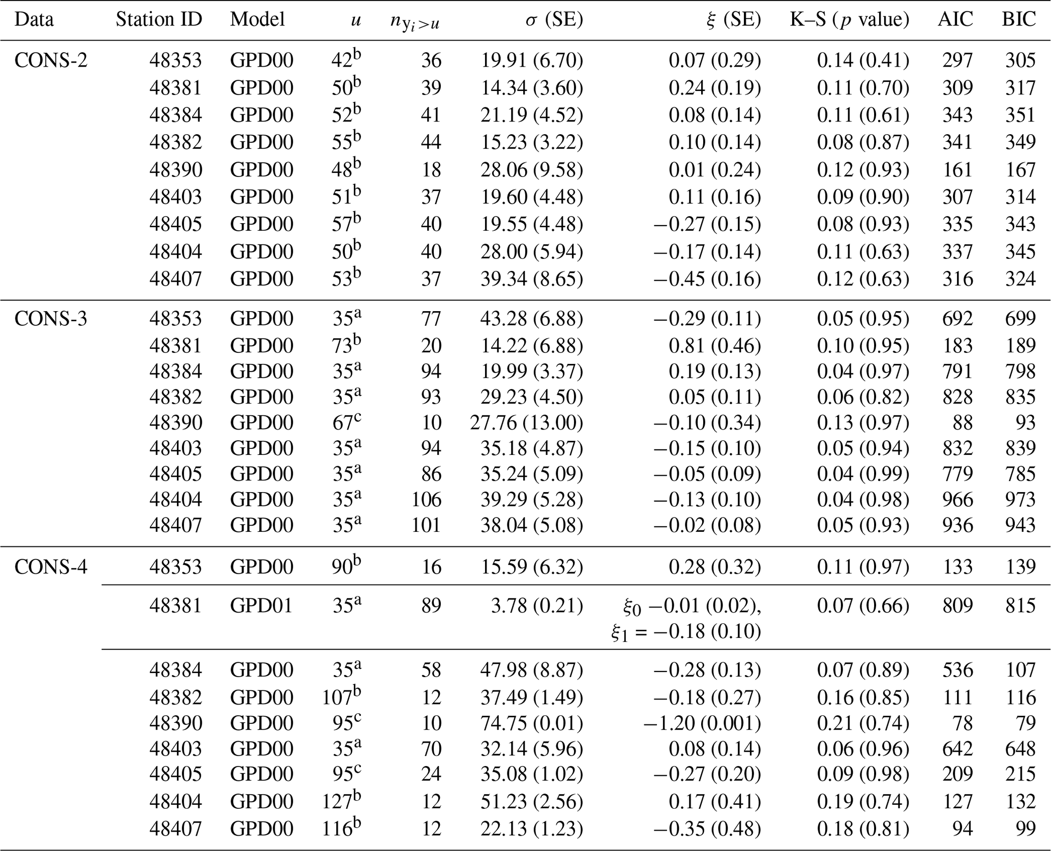
In the case of $n_{{\mathrm{y}}_i>u}<\mathrm{30}$, parameter estimates were obtained using the linear moment method. The threshold values u^a, u^b, and u^c represent the meteorological critical value, the 90th percentile of the data set, and the mean residual life (MRL) plot, respectively.

3.6 Return level

Return levels or quantiles are used to interpret extreme values in terms of their probability of return period. Once a suitable model has been defined, return levels can be calculated as follows:

$$\begin{array}{}\text{(6)}& {\widehat{Z}}_T=u+{\displaystyle \frac{\widehat{\mathit{\sigma }}}{\widehat{\mathit{\xi }}}}\left[(T{n}_{\mathrm{y}}{\widehat{\mathit{\lambda }}}_u{)}^{\widehat{\mathit{\xi }}}\right].\end{array}$$

It is a T-year return level, where n_y is the number of observations per year, and it corresponds to the t-observation return level $t=T\times n_{\mathrm{y}}$; and when ξ=0, the return level can be calculated as (Coles, 2001)

$$\begin{array}{}\text{(7)}& {\widehat{Z}}_T=u+\widehat{\mathit{\sigma }}\log \left(T{n}_{\mathrm{y}}{\widehat{\mathit{\lambda }}}_u\right),\end{array}$$

where ${\widehat{\mathit{\lambda }}}_u=k/n$ is the sample proportion of points exceeding u.

4 Results

In this study, the threshold method was employed to select the appropriate threshold u. To select the appropriate threshold u, we employed the threshold method in this study. The threshold values were determined based on the meteorological critical value (Meteorological, 2021), the 90th percentile of the data set, and the mean residual life (MRL) plot. Tables 4 and 5 present the estimated parameters for these models, which were obtained using both the maximum likelihood and linear moment methods.

Table 5 Parameter estimates and standard error (SE) with thresholds (u), the number of exceedances ($n_{{\mathrm{y}}_i>u}$), and the results of the goodness-of-fit test (p values) for the maximum cumulative rainfall of consecutive rainy days for 5, 6, and 7 d at selected stations. AIC: Akaike information criterion; BIC: Bayesian information criterion.

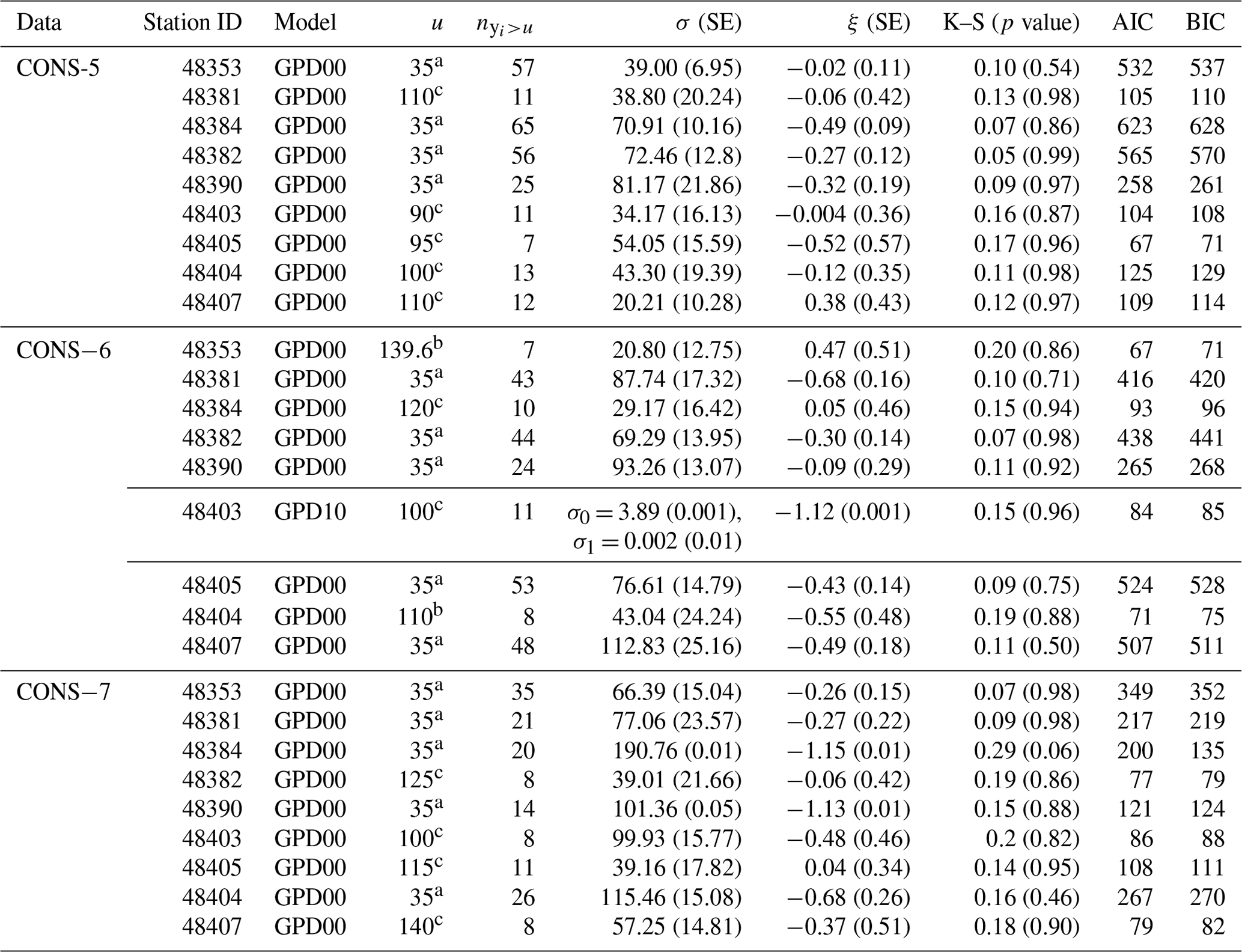
In the case of $n_{{\mathrm{y}}_i>u}<\mathrm{30}$, parameter estimates were obtained using the linear moment method. The threshold values u^a, u^b, and u^c represent the meteorological critical value, the 90th percentile of the data set, and the mean residual life (MRL) plot, respectively.

Parameter estimation employed both MLE and L-ME methods, depending on the number of exceedances ($n_{{\mathrm{y}}_i>u}$). The MLE was chosen when $n_{{\mathrm{y}}_i>u}\ge \mathrm{30}$, while L-ME was used when $n_{{\mathrm{y}}_i>u}<\mathrm{30}$. Standard errors were calculated using nonparametric bootstrap.

The data suitability for the GPD was confirmed via goodness-of-fit tests. Model selection relied on minimizing the Akaike information criterion (AIC) or the Bayesian information criterion (BIC) while ensuring that p values from K–S and AD tests were greater than 0.05 (p values: 0.06–0.994; see the details in Tables 4 and 5). The estimated scale and shape parameter ranges were (34.92, 124.45) and (−0.10, 0.16), respectively. These findings robustly endorsed the suitability of the GDP00 model for analyzing maximum cumulative rainfall on all CONS data. All stations, with the exception of the Khon Kaen (48381) station in CONS-4 data and Chaiyaphum (48403) station in CONS-6, exhibited the best fit to the GPD01 model, indicating that the shape parameters followed linear functions.

The return level estimates for CONS-2 and CONS-7 across various return periods in Tables 6 and 7 were computed using Eqs. (6) and (7). Bold values in the tables indicate the highest maximum cumulative rainfall return levels. In Table 6, the three stations with the highest return levels were Udon Thani (48354), Chok Chai (48434), and Khon Kaen (48381). As shown in Table 7, the three stations with the highest return levels were Sisaket (48409), Udon Thani (48354), and Ubon Ratchathani Agromet. (48408). These stations exhibited the highest cumulative rainfall return levels for all return periods compared with other stations. For CONS-3, CONS-4, CONS-5, and CONS-6, the results of estimates of the maximum cumulative rainfall return level can be found in the Supplement.

Table 6 Estimated return levels over various return period years, where the values in parentheses are standard error for maximum cumulative rainfall for CONS-2. The bold values present the first three stations which have maximum cumulative rainfall return level.

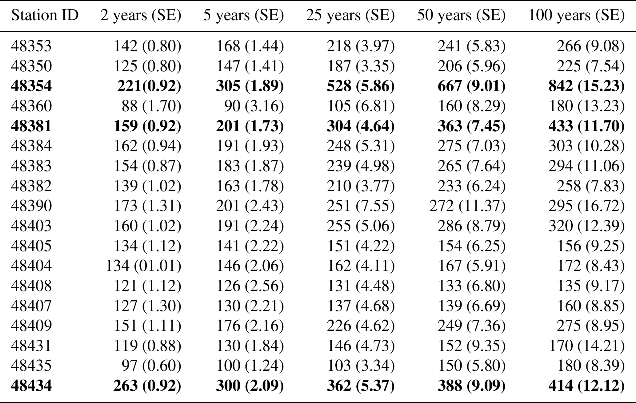
Table 7 Estimated return levels over various return period years, where the values in parentheses are standard error for maximum cumulative rainfall for CONS-7. The bold values present the first three stations which have maximum cumulative rainfall return level.

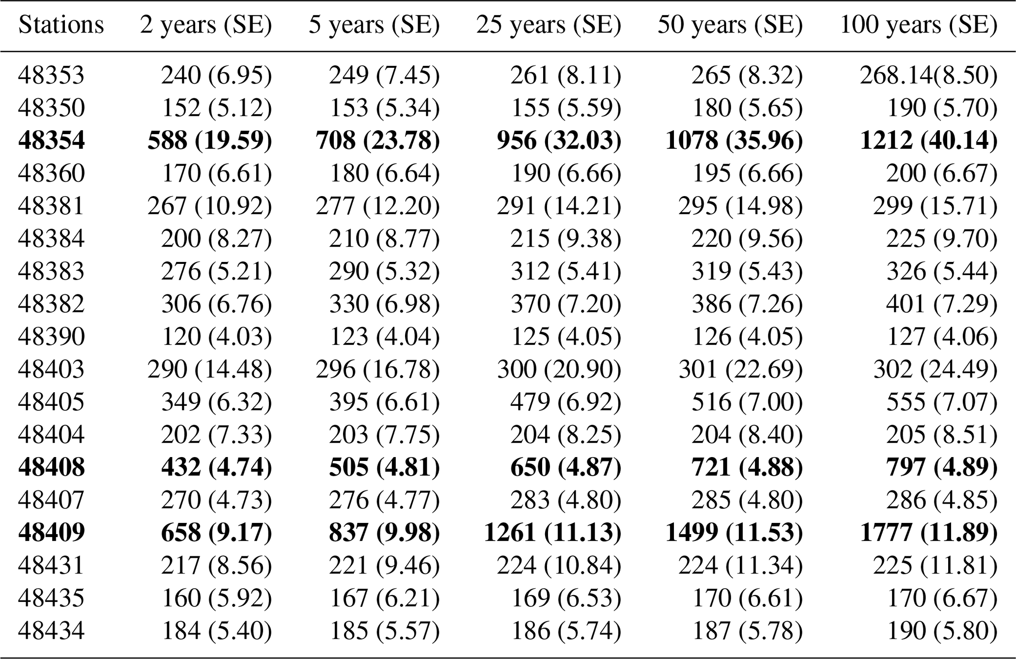
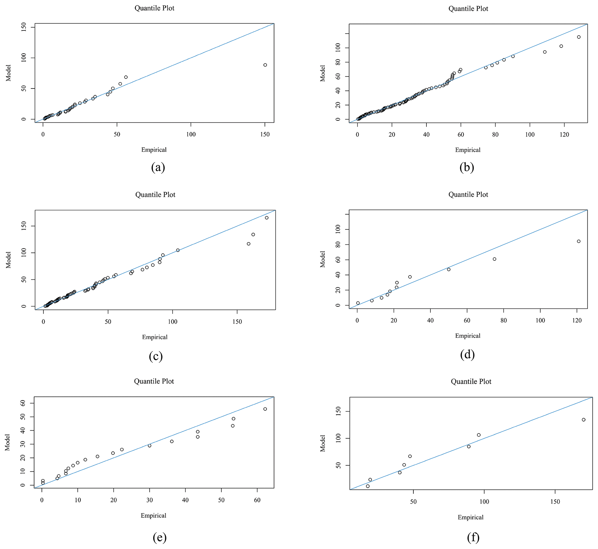
Figure 4 Panels (a)–(f) show quantile–quantile (QQ) plots for the maximum cumulative rainfall on consecutive rainy days for 2, 3, 4, 5, 6, and 7 d at Chaiyaphum meteorological station in the Chi watershed, northeastern Thailand. The x axis of the QQ plots represents the theoretical quantiles, while the y axis represents the observed quantiles.

Since Chaiyaphum Station is the origin station of the Chi watershed and a direct station, we present the quantile and return level plots of this station in Figs. 4–5. Figure 4 shows points falling on or near the diagonal line, indicating that the data follow the assumed distribution. Figure 5 illustrates the return level for return periods ranging from 0.005 to 5 years, determined using the profile likelihood method at Chaiyaphum Station.

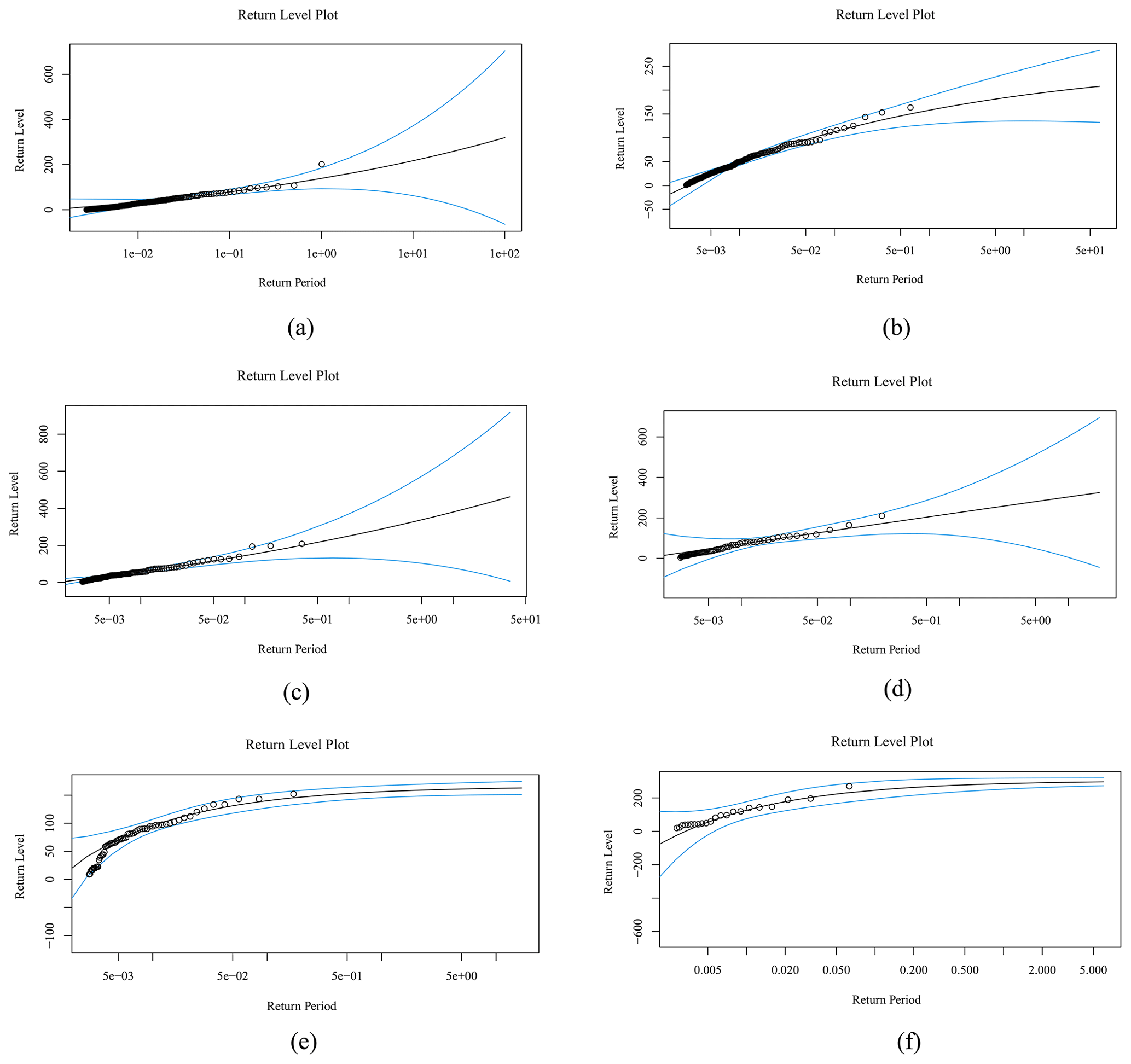
Figure 5 Panels (a)–(f) show return level plots (profile likelihood method) for the maximum cumulative rainfall on consecutive rainy days for 2, 3, 4, 5, 6, and 7 d at Chaiyaphum meteorological station in the Chi watershed, northeastern Thailand.

To enhance the visualization of the results, return level maps were generated using the Q-Geographic Information System (Q-GIS) program with the Inverse Distance Weighting (IDW) interpolation method. The IDW interpolation method assigns weights to the sample points based on their distance from the unknown point being interpolated. Figures 6 and 7 show the return level maps for CONS-2 and CONS-7, respectively.

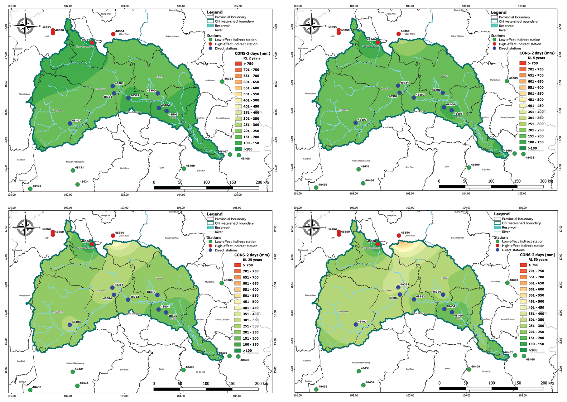
Figure 6 Estimated return level of maximum cumulative rainfall for 2 consecutive rainy days in the Chi watershed for 2-, 5-, 25-, and 50-year periods.

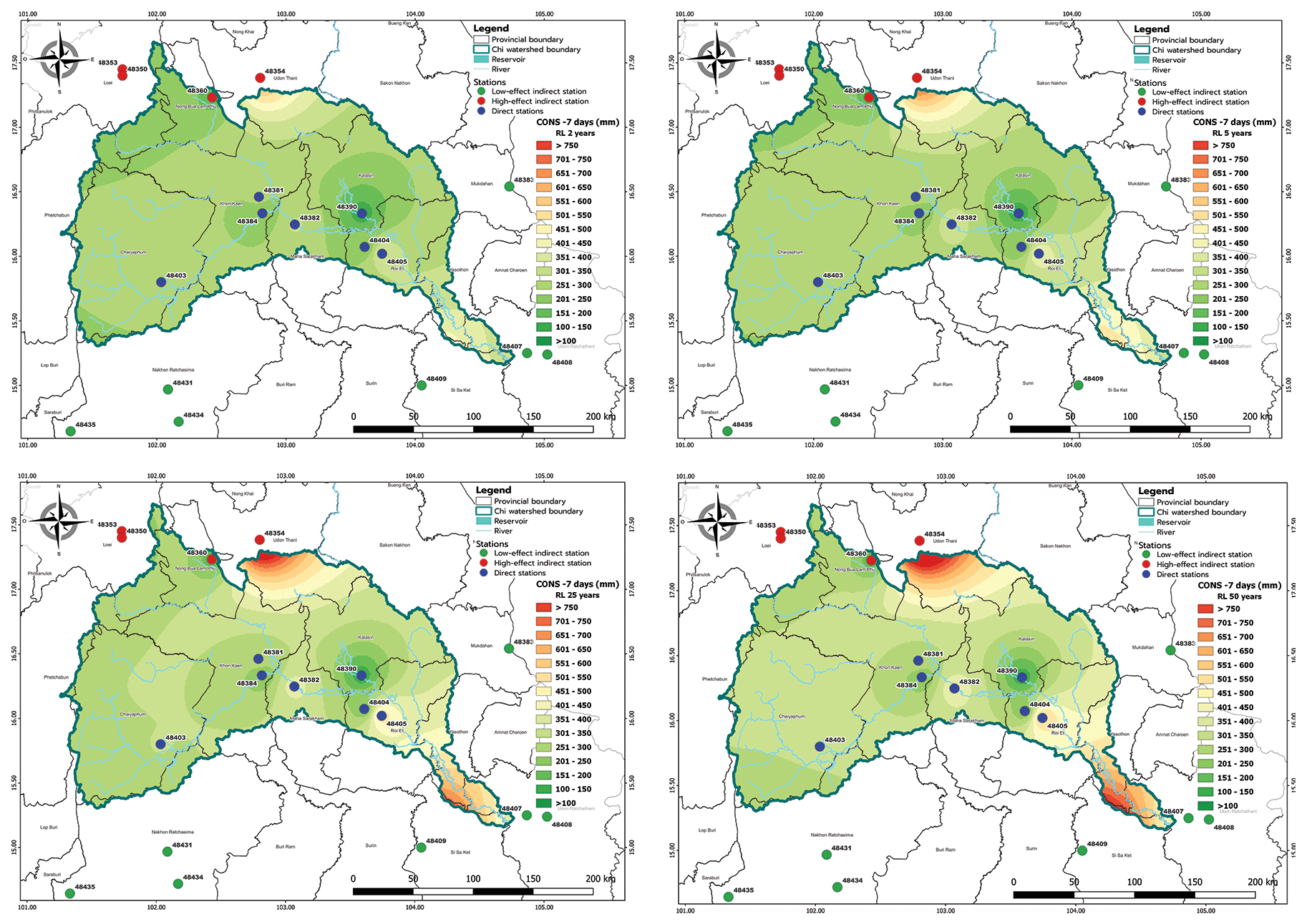
Figure 7 Estimated return level of maximum cumulative rainfall for seven consecutive rainy days in the Chi watershed for 2-, 5-, 25-, and 50-year periods.

Figures 6 and 7 present the spatial distribution of the estimated return levels of maximum cumulative rainfall for CONS-2 and CONS-7, respectively, for the return periods of 2, 5, 25, and 50 years. The results for the other CONS-3, CONS-4, CONS-5, and CONS-6 are presented in the Supplement. From the figures, it can be observed that Udon Thani (48354), Chaiyaphum (48430), Maha Sarakham (48382), Tha Phra Agromet. (48384), Roi Et (48405), and Sisaket (48409) had the highest return levels for all return periods of CONS-2 and CONS-7. This information can be useful for decision-making related to disaster risk management, such as identifying areas that are more vulnerable to extreme rainfall events and designing appropriate adaptation and mitigation strategies.

In addition, it can be observed that there was a significant difference in the return level for the 100-year period as compared with the other return periods in the figures of the maximum cumulative rainfall return level forecast for CONS-7 of rainfall data. The return level increased every year for all stations, indicating the importance of future rainfall management planning. These findings reveal the risk of flooding areas in the Chi watershed, including provinces such as Udon Thani, Chaiyaphum, Khon kaen, Maha Sarakham, Roi Et, and Sisaket. The figures were generated using the Q-GIS program, and they provide valuable insights into the spatial distribution of extreme rainfall events in the study area.

5 Discussion

In this study, the generalized Pareto distribution parameters were estimated using both maximum likelihood and L-moment estimation methods. Our decision to use MLE when the number of $n_{{\mathrm{y}}_i>u}\ge \mathrm{30}$ and L-ME was otherwise aligns with previous studies (Dupuis and Winchester, 2001; Papukdee et al., 2022), which also demonstrated the efficacy of these methods for different sample sizes. The consistency of our p values from K–S and AD tests with these studies further validates our modeling process.

We selected a threshold based on meteorological conditions, specifically when rainfall exceeded 35 mm, indicating heavy rainfall (Meteorological, 2021). This threshold, while higher than those used in some earlier studies, was deemed appropriate for our focus on extreme rainfall events. The range of scale and shape parameters estimated in our study were consistent with previous works in similar climatic zones (Phoophiwfa et al., 2023a), supporting the applicability of the GPD for extreme rainfall in our study area.

Our analysis pinpointed Udon Thani province as having the highest cumulative rainfall return levels across all return periods, signaling a heightened risk of flooding. This finding holds significant implications for future rainfall management planning, echoing the importance emphasized in prior research advocating for regionally specific flood risk assessment (Prahadchai et al., 2022). Expanding on previous work, our study presents estimated maximum cumulative rainfall return levels for CONS-2 and CONS-7 events at selected stations. This detailed analysis offers guidance for targeted flood mitigation efforts, particularly in regions such as Udon Thani, Chaiyaphum, and Sisaket identified as higher-risk areas.

The utilization of Q-GIS to create return level maps via the inverse distance weight (IDW) interpolation method provides a visually intuitive depiction of flood risk spatial distribution. While common in geographic analysis, this application in mapping extreme rainfall return levels is, to our knowledge, a pioneering instance (Flenniken et al., 2020).

Our findings emphasize the necessity for future rainfall management planning specifically within the Chi watershed. This study can be extended beyond the Chi watershed by examining the potential impact of its findings on policy formulation, infrastructure planning, and disaster mitigation strategies in regions confronted with analogous challenges. Broadening the scope, the research probes the implications of its results for the domains of hydrology, climatology, and environmental science.

Numerous organizations, including prominent bodies like the IPCC (IPCC, 2014) and UNFCCC (UNFCCC, 2015), are increasingly acknowledging the pervasive challenges posed by climate change. This global phenomenon manifests in widespread impacts, affecting temperatures and altering the frequency and intensity of extreme weather events (Bridhikitti et al., 2023).

Nonetheless, our study acknowledges certain limitations, notably the assumption of stationary rainfall patterns, which may, however, be influenced by climate change. Future research could delve into the impact of changing climate conditions on extreme rainfall events, thereby refining models to accommodate a warming climate.

6 Conclusions

This study set out to evaluate extreme rainfall events in the Chi watershed in northeastern Thailand with the aim of applying extreme value theory to predict future rainfall patterns. We analyzed maximum cumulative rainfall data from 1984 to 2018 and fitted the generalized Pareto distribution to the data. This model was determined to be appropriate through goodness-of-fit tests, providing a robust method for analyzing extreme rainfall events in the region. Our results reveal that Udon Thani, Chaiyaphum, Maha Sarakham, Tha Phra Agromet., Roi Et, and Sisaket provinces had the highest return levels for CONS-2 and CONS-3, suggesting that these areas are at high risk of flooding.

These findings underscore the importance of forecasting and planning for extreme rainfall events in the Chi watershed. We found that even short periods of continuous rainfall could lead to flash flooding, highlighting the need for effective water management in the region. We also developed 2D maps, which provide a practical tool for visualizing at-risk areas and aiding in the planning of soil and water conservation measures, dam construction, as well as irrigation and drainage work.

The implications of this study extend beyond academia. Our findings provide valuable insights for governmental agencies, private organizations, and individuals alike, empowering them to design more effective flood management strategies, thereby reducing the risk and potential impact of flooding in their communities. In the broader context, managing extreme rainfall events and mitigating flood risks are crucial for safeguarding property, preserving ecosystems, and ultimately saving lives.

Future research should explore spatial analysis to determine interdependencies among different regions and use copula functions for correlation analysis. Such developments could provide a more nuanced understanding of the region's flood risk and further enhance our ability to predict and prepare for extreme rainfall events.

In conclusion, this study underscores the urgency of focusing on extreme rainfall events in our fight against the increasing threat of flooding. With climate change intensifying, the tools and strategies we develop today will be instrumental in managing the water-related challenges of tomorrow.