Modeling hydropower operations at the scale of a power grid: a demand-based approach

Climate change and evolving water management practices may have a significant impact on hydropower generation. While hydrological models have been widely used to assess these effects, they often present some limitations. A major challenge lies in modeling the release decisions for hydropower reservoirs, which result from intricate trade-offs, involving power sector dispatch, competing water uses, and the spatial allocation of power generation within the grid.

To address this gap, this study introduces a novel demand-based approach for integrating hydropower within the routing module of land surface models. First, hydropower infrastructures are located in coherence with the hydrological network, and links are built between hydropower plants and their supplying reservoirs to explicitly represent water transfers built for hydropower generation. Then, coordinated dam operation is simulated by distributing a prescribed electric demand to be satisfied by hydropower across the different power plants within the power grid, while considering the operational constraints associated with the multipurpose nature of most dams.

To validate this approach, we implement the framework within the water transport scheme of a land surface model and assess it with the case study of the French electrical system. We drive the model with a high-resolution atmospheric reanalysis and prescribe the observed national hydropower production as the total power demand to be met by hydropower infrastructures. By comparing the simulated evolution of reservoir stocks to observations, we find that the model simulates realistic operations of reservoirs and successfully satisfies hydropower production demands over the entire period. We also highlight the roles of uncertainties in estimated precipitation and of the limited knowledge of hydropower infrastructure in the estimation of production. Finally, we show that such an integration of hydropower operations in the model improves the simulations of river discharges in mountainous catchments affected by hydropower.

1 Introduction

1.1 Background and motivation

Hydroelectric power is set to play a pivotal role in numerous power grids in the coming decades, offering low-carbon and dispatchable generation capacity. However, power grids that rely on hydropower production are vulnerable to the unpredictability of weather and climate. Consequently, assessing the potential impact of drought events or climate change on hydropower production is a major concern for the development of resilient energy systems.

Numerous studies (Lehner et al., 2005; Van Vliet et al., 2016; Turner et al., 2017; Zhou et al., 2018; Voisin et al., 2020) have revealed significant impacts of climate change on hydropower production in certain regions, including southwestern Europe and France. These studies typically employ global hydrological models (GHMs) or land surface models (LSMs) driven by atmospheric projections generated by global climate models (GCMs) (Turner and Voisin, 2022). These models simulate the regional-scale hydrological cycle, offering gridded assessments of surface runoff and streamflow, which are then used to derive hydropower production estimates.

However, the estimation process from streamflow to hydropower production is challenging for three reasons. Firstly, water can be stored in reservoirs for future use. The timing of reservoir releases is then the result of the management of the power grid and the coordinated operation of other plants across various water catchments. Secondly, reservoirs that feed hydropower plants are often multipurpose and operated to satisfy other water uses, namely irrigation or tourism. Thirdly, hydropower production can involve inter-catchment water transfers, particularly in mountainous regions where water is stored at higher elevations before being channeled to power plants located in the valleys.

Existing studies adopt diverse strategies to represent these complex operations of hydroelectric reservoirs, which are generally categorized into two main approaches (Nazemi and Wheater, 2015b). On the one hand, simulation algorithms rely on predefined rules to compute reservoir releases. These rules are often a function of reservoir inflow and filling level, inspired by the pioneering work of Hanasaki et al. (2006) (e.g. in MOSART-WM, a reservoir scheme used by Zhou et al. (2018), Voisin et al. (2020), and Ralston Fonseca et al. (2021)). They can also be defined based on target curves of water levels from which the release is determined (e.g. in VIC-RES (Dang et al., 2020) used by Chowdhury et al. (2021) and Siala et al. (2021)). Such methods account for the seasonal behavior of hydroelectric reservoirs, but they miss the representation of short-term operations, as no links with the power system needs are made. On the other hand, optimization algorithms based on the pioneering work of Haddeland et al. (2006) determine the optimal release for each dam. The objective function to optimize varies depending on the reservoir's primary purpose, aiming to maximize individual production for hydroelectric reservoirs. However, this method considers each reservoir independently and often employs large time steps (monthly) to reduce computational strain.

When the models differentiate the various uses of reservoirs, they categorize the reservoirs based solely on their primary purpose (Abeshu et al., 2023). This approach does not allow the full range of constraints to be captured that apply to most hydroelectric reservoirs, which are often multipurpose. Moreover, none of these studies operate the dams as a network that takes advantage of the spatial complementarity of different climatic regions or the cascading effects within river systems.

Finally, none of these large-scale studies explicitly model the water transfers from reservoirs to power plants. In most cases, the flow rate within the grid cell where the power plant is located is used to estimate its production, without considering the actual location of the reservoir (Van Vliet et al., 2016; Zhou et al., 2018; Voisin et al., 2020). This approach may lead to an overestimation of production, as the flow rate at the plant site is higher than at an upstream dam site, and inter-basin transfers may also occur.

1.2 Objectives

The objective of this study is to present the original methodology we developed to estimate hydropower production at the scale of a regional power grid. This approach is based on the simulations of a GHM or LSM and addresses the three challenges previously identified: (i) considering the coordinated management of the entire power system at the scale of the power grid, (ii) accounting for the multipurpose objectives of reservoirs that store water for hydropower production, and (iii) representing the inter-catchment water transfers from reservoirs to power plants.

Our approach draws inspiration from the demand-based algorithms used for irrigation reservoir management, pioneered by Hanasaki et al. (2006). In these algorithms, a demand point (irrigated area) is connected to a supply point (river), with the water demand of the downstream irrigated area driving upstream reservoir releases (Nazemi and Wheater, 2015b; Zhou et al., 2021).

In our methodology, hydropower plants are linked to reservoirs whose releases depend on the demand for hydropower production. At the geographical scale of the whole power grid, the primary concern is balancing total electricity demand with generation, regardless of the specific locations of consumption and generation. Consequently, we assume that all hydroelectric reservoirs within the power grid can contribute to satisfying the demand for dispatchable hydropower production, determined by grid-level power system dispatch decisions. Power dispatching involves deciding which types of power plants are activated to satisfy the total power demand, based on the cost and availability of generation resources. Our model does not explicitly represent this side of the power system decisions but uses the corresponding demand for dispatchable hydropower to drive the operation of the hydroelectric reservoirs.

We implement the proposed methodology in the ORCHIDEE LSM (Krinner et al., 2005), but it is the aim that it is usable in any LSM or GHM. The first steps involve building a river network that represents inter-catchment hydropower transfers and defining rules for reservoir releases. These steps are generic and only require basic information on dam and plant characteristics. To validate the effectiveness of the approach, we apply it to the French power grid. A calibration step is added, which requires more information on individual plants. Finally, the simulated operations of hydroelectric reservoirs are compared with actual operations.

The paper is structured as follows: Sect. 2 describes the proposed methodology and its originality. Section 3 introduces the data and methods used for the French power grid case study and assesses the performance of ORCHIDEE in reproducing river discharges over this area. Section 4 presents the modeling results, and finally Sect. 5 discusses these results and concludes by outlining future perspectives of research.

2 Model

Our method relies on three main novelties: building a river network that includes hydropower-related infrastructures and represents inter-basin hydropower transfers (Sect. 2.1), implementing a reservoir scheme that accounts for multipurpose reservoirs (Sect. 2.2), and using hydropower demand to infer hydroelectric reservoir operations (Sect. 2.3).

2.1 Definition of a routing network that includes hydropower connections

The spatial resolution of GHMs or LSMs is typically constrained by the atmospheric grid of the forcing files, which is generally set at 0.5° (approximately 50 km) for large-scale implementations and 0.1° (approximately 10 km) for regional implementations. However, human activities, such as irrigation or urban areas, operate at much finer spatial resolutions, typically within a few kilometers. The concept of hydrological transfer units (HTUs) has been introduced in routing modules to bridge this resolution gap (Nguyen-Quang et al., 2018). HTUs correspond to sub-grid river basins, which allow runoff generated in one atmospheric grid cell to flow into multiple neighboring cells. The introduction of these smaller units allows for a more accurate representation of the river system and its interaction with human activities, including hydropower.

Three types of hydropower plants are distinguished, with different implications for locations:

• Run-of-river plants do not have any storage capacity and generate electricity according to the instantaneous river discharge at the plant location.

• Reservoir plants are fed by reservoirs that can store a specified water volume. These reservoirs often serve multiple purposes, which may constrain the operations of the plant. The electricity production does not necessarily take place at the location of water storage; therefore the plant and the reservoir need to be located separately on the model grid.

• Poundage plants are defined in some regions as a subcategory of reservoir plants whose upstream reservoir is relatively small and only allows water to be stored for a short period.

As an example of different locations of reservoir and power plant, the “La Bâthie” power plant, the largest reservoir power plant in France, draws water from the Roselend reservoir, which is located about 20 km away (see Appendix D). At a kilometric resolution, this implies horizontal water transfers between these two locations (water withdrawal and restitution), which require the reconstruction of the hydroelectric water supply network within the routing network of ORCHIDEE.

We proceed in three steps, as illustrated in Fig. 1. First (Fig. 1b), we place dams and hydropower plants on a high-resolution river network (MERIT (Yamazaki et al., 2019) is used in this study), based on georeferenced data and upstream area provided in infrastructure databases. The location procedure is detailed in Appendix A, and the infrastructure datasets used for our study of France are presented in Appendix B. Then, we build the adduction network by identifying supposed connections between power plants and dams that feed them (see Appendix A for more details on the procedure to build the adduction network). Finally (Fig. 1c), we form HTUs by aggregating MERIT pixels in an atmospheric grid cell with the same general flow direction following the procedures described in Nguyen-Quang et al. (2018) and Polcher et al. (2023).

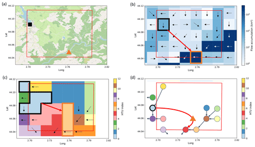
Figure 1 Illustration of the procedure to build the ORCHIDEE routing network using the Pouget hydropower plant in France as an example. (a) Geographic context of the Pouget power plant (orange triangle) and its feeding reservoir (black square indicating the location of the dam). The red grid indicates the atmospheric grid. (b) Flow directions and accumulation for the MERIT pixels overlapping the atmospheric grid. The MERIT pixels in which we located the power plant and the dam are, respectively, indicated in orange and black, while the red arrow represents the identified adduction network link. (c) Resulting HTU decomposition. The location of the infrastructures is reported in the corresponding HTUs. (d) Corresponding HTU graph. The HTU containing the dam is indicated with a bold black outline, while the power plant (orange triangle) is placed on the edge between the reservoir HTU and the HTU downstream from the one where it has been located.

This procedure results in an HTU network representing natural and human-made water flows. This network can be seen as a directional graph (Fig. 1d) where vertices correspond to HTUs and edges represent directional water flows, both natural and human-made flows for hydropower purposes. In this graph, hydropower plants are placed on the edges connecting the HTU of their withdrawal point and the HTU downstream where they are located. Figure 2 introduces the notation that will be used throughout the article to index HTUs and edges in such graphs. It shows that the water used to produce electricity can follow a different path from the natural flow out of the reservoir. This approach allows for the representation of this distinction independently of the atmospheric resolution.

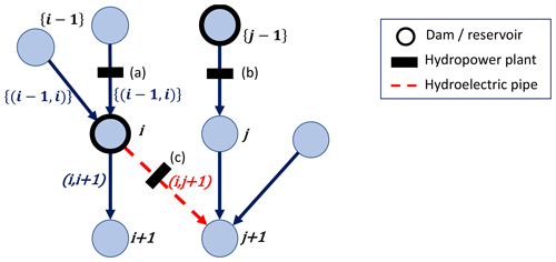
Figure 2 Graph representation of the river routing network built. Each vertex represents an HTU. HTUs containing a dam are represented by bold dark circles. Edges represent existing water flow directions (blue edges for natural water flows and dashed red ones for hydroelectric pipes). Power plants are placed on edges whose water flows they can use to produce power (a) Run-of-river plant and (b, c) reservoir or poundage plants. The indexing convention is also presented on the graph, with integers used for vertices and couples of integers for edges. i+1 is the HTU directly downstream of i (natural flow), while {i−1} denotes the ensemble of HTU flowing into HTU i. Similarly $(i,i+\mathrm{1})$ is the natural outflow edge from HTU i, while $\mathit{\left\{}\right(i-\mathrm{1},i\left)\mathit{\right\}}$ represents the ensemble of inflow edges into HTU i, including basin transfers.

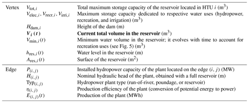
The attributes and variables describing the reservoir and hydropower characteristics of each HTU i and vertex (i,j) are presented in Table 1.

Table 1 Model attributes and variables describing reservoirs and hydropower. The prognostic variable is distinguished in bold.

During calibration (see Sect. 2.5), plants for which the identification of a single reservoir conducts a significant misrepresentation of the plant's hydropower potential are identified, and a correction is made by moving the withdrawal point so that it gathers enough water to ensure the observed production is possible.

2.2 Dam and reservoir parametrization

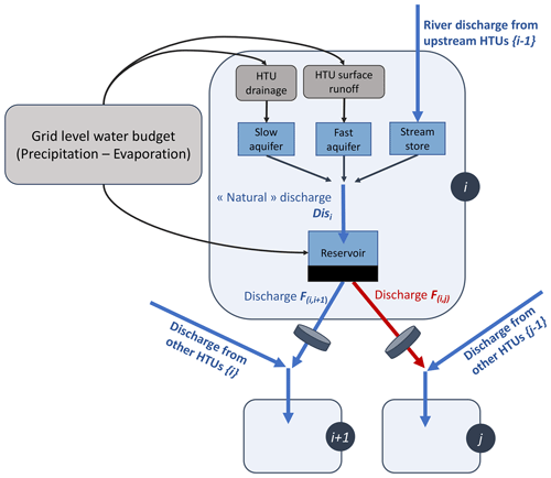
In the initial version of ORCHIDEE (Polcher et al., 2023), each HTU i contains three natural water stores, characterized by their time constants (slow aquifer, fast aquifer, and stream storage). To represent water management, we add a fourth store to the HTUs in which dams have been located to represent water storage in the reservoir (Fig. 3). This section presents the continuity equation for the water volume in this reservoir.

Figure 3 Schematic representation of water stores and flows in HTU i.

2.2.1 Prognostic equation for water in the reservoir

As represented in Fig. 3, the fast aquifer is filled by local runoff generated in the HTU, the slow aquifer by local drainage generated in the HTU, and the stream store by the discharge from upstream HTUs. The equations of these natural water stores are detailed in previous publications (Zhou et al., 2021; Polcher et al., 2023). They introduce the respective time constants of the natural stores, g_stream, g_fast, and g_slow (in unit h m⁻¹), and the topographic index calculated for each HTU τ_i (in unit m²).

The “natural discharge” Dis_i(t) in HTU i is generated by summing the outflows of the three natural water stores (Eq. 1). This natural discharge is stored in the reservoir if there is one in the HTU or routed towards the downstream HTU if there is not.

$$\begin{array}{}\text{(1)}& {\mathrm{Dis}}_i\left(t\right)={\displaystyle \frac{\mathrm{1}}{{\mathit{\tau }}_i}}\cdot \left({\displaystyle \frac{W_{\mathrm{stream},i}\left(t\right)}{g_{\mathrm{stream}}}}+{\displaystyle \frac{W_{\mathrm{fast},i}\left(t\right)}{g_{\mathrm{fast}}}}+{\displaystyle \frac{W_{\mathrm{slow},i}\left(t\right)}{g_{\mathrm{slow}}}}\right)\end{array}$$

The prognostic equation on reservoir volume is then given by

$$\begin{array}{}\text{(2)}& {\displaystyle \frac{\mathrm{d}{V}_i}{\mathrm{d}t}}\left(t\right)={\mathrm{Dis}}_i\left(t\right)+p_{\mathrm{res},i}\left(t\right)-{\mathrm{ev}}_{\mathrm{res},i}\left(t\right)-\sum _j{F}_{(i,j)}\left(t\right),\end{array}$$

where p_res,i(t) and ev_res,i(t) are, respectively, the direct precipitation and evaporation over the reservoir, and F_(i,j)(t) is the water released from HTU i to HTU j, which breaks down as

$$\begin{array}{}\text{(3)}& F_{(i,j)}\left(t\right)=max\left(F_{(i,j)}^{\mathrm{ecol}}\left(t\right),F_{(i,j)}^{\mathrm{irri}}\left(t\right),F_{(i,j)}^{\mathrm{elec}}\left(t\right)\right)+F_{(i,j)}^{\mathrm{spill}}\left(t\right).\end{array}$$

Reservoir releases aim at satisfying the different water demands addressed to the reservoir, which are described in Sect. 2.3. Ecological and irrigation releases are limited by the demands addressed to the reservoir and the water available in the reservoir:

$$\begin{array}{}\text{(4)}& {\displaystyle }{F}_{(i,j)}^{\mathrm{ecol}}\left(t\right)=min\left(D_{(j,i)}^{\mathrm{ecol}}\left(t\right),{\displaystyle \frac{V_i^{\star }\left(t\right)-V_{\min ,i}\left(t\right)}{{\mathit{\tau }}_{\mathrm{res}}}}\right)\text{(5)}& {\displaystyle }{F}_{(i,j)}^{\mathrm{irri}}\left(t\right)=min\left(D_{(j,i)}^{\mathrm{irri}}\left(t\right),{\displaystyle \frac{V_i^{\star }\left(t\right)-V_{\min ,i}\left(t\right)}{{\mathit{\tau }}_{\mathrm{res}}}}\right),\end{array}$$

where $V_i^{\star }\left(t\right)$ is the theoretical volume to be obtained without any release (Eq. 6) and τ_res is the time constant of the reservoir, which we assume to be of the order of magnitude of a few minutes.

$$\begin{array}{}\text{(6)}& {\displaystyle \frac{\mathrm{d}{V}_i^{\star }}{\mathrm{d}t}}\left(t\right)={\mathrm{Dis}}_i\left(t\right)+p_{\mathrm{res},i}\left(t\right)-{\mathrm{ev}}_{\mathrm{res},i}\left(t\right)\end{array}$$

The water released for electricity generation is determined by the production of the plant, computed based on the distribution of the prescribed national demand (see Sect. 2.3).

$$\begin{array}{}\text{(7)}& F_{(i,j)}^{\mathrm{elec}}\left(t\right)={\displaystyle \frac{E_{(i,j)}\left(t\right)}{\mathit{\rho }g{\mathit{\eta }}_{(i,j)}{h}_{(i,j)}\left(t\right)}},\end{array}$$

where ρ is the water density; g is the gravitational constant; η_(i,j) is the efficiency of the plant (set at 0.9 by default); and h_(i,j)(t) is the current hydraulic head, which varies with the water level of the reservoir (Eq. 8).

$$\begin{array}{}\text{(8)}& h_{(i,j)}\left(t\right)=H_{(i,j)}-\left(H_{\mathrm{dam},i}-H_{\mathrm{res},i}\left(t\right)\right)\end{array}$$

Finally, the spillage is defined as the water overflowing without being used for the different uses.

$$\begin{array}{}\text{(9)}& {\displaystyle }{F}_{(i,j)}^{\mathrm{spill}}\left(t\right){\displaystyle }=\left\{\begin{array}{l}max\left(\frac{V_i^{\star }\left(t\right)-V_{\mathrm{tot},i}}{{\mathit{\tau }}_{\mathrm{res}}}-\sum _{k}max\right.\\ \left.\left(F_{(i,k)}^{\mathrm{ecol}}\left(t\right),F_{(i,k)}^{\mathrm{irri}}\left(t\right),F_{(i,k)}^{\mathrm{elec}}\left(t\right)\right),\mathrm{0}\right)& ,\mathrm{if}j=i+\mathrm{1}\\ \mathrm{0}& ,\text{else}.\end{array}\right.\end{array}$$

Ecological and irrigation flows $F_{(i,j)}^{\mathrm{ecol}}\left(t\right)$ and $F_{(i,j)}^{\mathrm{irri}}\left(t\right)$ are computed before the other flows, consistently with water management policy in most of the countries.

2.2.2 Diagnostic variables

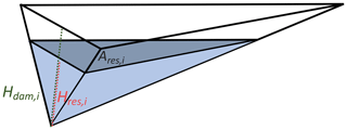
As in previous studies (Fekete et al., 2010; Zhou et al., 2018), we represent each reservoir i in the form of a tetrahedron of height H_dam,i and volume V_tot,i (Fig. 4).

Figure 4 Geometry of the reservoir.

Hence, the relations between the volume V_i(t), the water level H_res,i(t), and the area of the reservoir A_res,i(t) are given by

$$\begin{array}{}\text{(10)}& {\displaystyle }{H}_{\mathrm{res},i}\left(t\right)& {\displaystyle }=H_{\mathrm{dam},i}\cdot {\left({\displaystyle \frac{V_i\left(t\right)}{V_{\mathrm{tot},i}}}\right)}^{\frac{\mathrm{1}}{\mathrm{3}}}\text{(11)}& {\displaystyle }{A}_{\mathrm{res},i}\left(t\right)& {\displaystyle }={\displaystyle \frac{\mathrm{3}\cdot V_i\left(t\right)}{H_{\mathrm{res},i}\left(t\right)}}.\end{array}$$

Direct precipitation and evaporation (m³ s⁻¹) over the reservoir are then given by $p_{\mathrm{res},i}\left(t\right)=P_i\left(t\right)\cdot A_{\mathrm{res},i}\left(t\right)$ and ${\mathrm{ev}}_{\mathrm{res},i}\left(t\right)={\mathrm{Ev}}_i\left(t\right)\cdot A_{\mathrm{res},i}\left(t\right)$, where P_i(t) and Ev_i(t) are, respectively, the precipitation and evaporation over HTU i (in m s⁻¹).

2.3 Water demands

Reservoirs are designed to store water for a variety of purposes, including energy production, irrigation, tourism, and domestic and industrial uses. As this study focuses on hydroelectric reservoirs, we adopt a simplistic representation of the other water uses and only consider those that can constrain hydropower operations: ecological flows, irrigation, and tourism.

2.3.1 Non-energy demands

In many countries, environmental laws require a minimum flow $F_{\min ,(i,i+\mathrm{1})}$ in the watercourse downstream of a dam in i to guarantee the ecological quality of the river. These minimum flow requirements vary by region, and specific details for the French study case are presented in Sect. 3.3.1. Such an ecological demand $D_{(j,i)}^{\mathrm{ecol}}\left(t\right)$ applies to all reservoirs, regardless of their intended use, and is defined as follows:

$$\begin{array}{}\text{(12)}& D_{(j,i)}^{\mathrm{ecol}}\left(t\right)=\left\{\begin{array}{ll}{F}_{\min ,(i,i+\mathrm{1})},& \text{if}j=i+\mathrm{1}\\ \mathrm{0},& \text{else}.\end{array}\right.\end{array}$$

In addition to ecological requirements, some reservoirs are used for irrigation purposes. Water withdrawals for irrigation can be made either directly from the reservoir or from the downstream river. Withdrawals from the river require corresponding releases from upstream reservoirs to maintain low flows. In this study, the water requirements for irrigation are represented in a highly simplified manner by assuming a need proportional to $F_{\min ,(i,i+\mathrm{1})}$ during the summer period. $D_{(j,i)}^{\mathrm{irri}}\left(t\right)$ is then expressed as

$$\begin{array}{}\text{(13)}& D_{(j,i)}^{\mathrm{irri}}\left(t\right)=\left\{\begin{array}{ll}{\mathit{\alpha }}_{\mathrm{irri}}\cdot F_{\min ,(i,i+\mathrm{1})},& \text{if}j=i+\mathrm{1}\\ & and{V}_{\mathrm{irri},i}>\mathrm{0}\\ & andt\in \mathrm{summer}\\ \mathrm{0},& \text{else}.\end{array}\right.\end{array}$$

The proportional factor α_irri and the delimitation of the summer period may vary across regions. Details for the French case study are presented in Sect. 3.3.1.

Finally, during the summer months, some reservoirs also serve as tourist attractions, requiring the reservoir to be maintained at a high level to accommodate recreational activities. To ensure proper reservoir filling during the summer season, dam operators follow a filling guide curve. We define corresponding constraints on V_min,i(t) based on previous research and available data for French reservoirs (e.g. François (2013) on the Serre Ponçon reservoir), as illustrated in Fig. 5. By default, the minimum volume is set at 10 % of the total capacity of the reservoir and is increased to 90 % during the tourist season for the reservoirs concerned.

Figure 5 Minimum volume constraints throughout the year.

2.3.2 Hydroelectric demand

The production of hydropower plants is the result of the dispatch of the total power demand among the different power plants within the power grid (Stoft, 2002; Wood et al., 2013). To meet power demand at minimum cost, power generation units are called upon from the least to the most expensive. Run-of-river power plants, whose production is free and non-dispatchable, are called upon first, along with solar and wind power plants, to produce to their maximum potential (as long as it does not exceed total demand, otherwise there is a curtailment of their production). Conversely, the call upon reservoir power plants is the result of a much more complex trade-off, aiming to minimize the total power system cost. From the perspective of a social planner, in charge of dispatch decisions and aware of the potentials and costs of all the units available within the power grid, as well as the electricity demand, a demand for dispatchable hydropower generation D_res(t) can be defined at each time step. This demand (or production target) is defined for the whole grid and then needs to be allocated among the different plants to determine the energy generated at each location E_(i,j)(t), which will then drive reservoir release decisions. Indeed, knowing E_(i,j)(t), the model deduces the additional water release needed for the plant production (Eq. 7) and can finally compute the reservoir release based on Eq. (3).

To distribute national demand D_res(t) into individual plant production E_(i,j)(t), the model proceeds in two steps.

1. Fatal production. The model starts by going through all the hydropower plants and calculates the energy they can produce or store without additional release, thanks to other releases (ecological or irrigation) or the water expected to overflow. Associated production, $E_{\mathrm{fatal},(i,j)}\left(t\right)$ and $E_{\mathrm{spill},(i,j)}\left(t\right)$, is computed based on Eqs. (14) and (15).

   $$\begin{array}{}\text{(14)}& {\displaystyle }\begin{array}{rl}{E}_{\mathrm{fatal},(i,j)}\left(t\right)=& min(P_{(i,j)}{\displaystyle \frac{h_{(i,j)}\left(t\right)}{H_{(i,j)}}},\\ & max\left(F_{\mathrm{ecol},(i,j)}\right(t),F_{\mathrm{irri},(i,j)}(t\left)\right)\\ & \times \mathit{\rho }g{\mathit{\eta }}_{(i,j)}{h}_{(i,j)}\left(t\right))\end{array}\text{(15)}& {\displaystyle }\begin{array}{rl}{E}_{\mathrm{spill},(i,j)}\left(t\right)=& min(P_{(i,j)}{\displaystyle \frac{h_{(i,j)}\left(t\right)}{H_{(i,j)}}}-E_{\mathrm{fatal},(i,j)}(t),\\ & max({\displaystyle \frac{V_i^{\star }\left(t\right)-V_{\mathrm{tot},i}}{{\mathit{\tau }}_{\mathrm{res}}}}\\ & -max\left(F_{\mathrm{ecol},(i,i+\mathrm{1})}\right(t),\\ & F_{\mathrm{irri},(i,i+\mathrm{1})}\left(t\right)),\mathrm{0})\\ & \times \mathit{\rho }g{\mathit{\eta }}_{(i,j)}{h}_{(i,j)}\left(t\right))\end{array}\end{array}$$

   The remaining production demand to dispatch is then $D_{\mathrm{res}}\left(t\right)-{\sum }_{Typ(i,j)\in \mathit{\{}\mathrm{poundage},\mathrm{reservoir}\mathit{\}}}\left(E_{\mathrm{fatal},(i,j)}\right(t)+E_{\mathrm{spill},(i,j)}(t\left)\right)$.

2. Reservoir withdrawals. If there is any national production demand left to dispatch (D_res(t) > 0), it should be met by withdrawing water from the reservoirs. In this study, we consider that the reservoirs are used in the decreasing order of their relative filling levels to produce power while respecting production constraints (installed capacity of the plant and the remaining volume of water in the reservoir). The remaining production is dispatched following this rule, until either all remaining production demand is fulfilled, or no more plants can produce. This rule leads to the equalization of relative filling levels at the end of each time step. This is equivalent to implementing a uniform rule curve for all reservoirs, as has been done in Dang et al. (2020). Another advantage of this rule is that hydropower production is distributed across the entire territory. All plants are required to produce a little power each day, close to the so-called stable production modeled in other studies (Sterl et al., 2020).

2.4 Validation diagnostics

The performance of our model to estimate hydropower production will be assessed based on three main diagnostics: the annual hydropower potential (AHP) simulated at each individual plant, the hydraulic stock simulated at the national level, and the time series of simulated production by hydropower plant type.

We define AHP_(i,j)(y) as the maximum energy that could be produced by the plant (i,j) over the year y in our simulation. To compute it, we run a simulation in which the demand for dispatchable hydropower D_res(t) is fixed to infinite, leading all hydroelectric reservoirs to release water within the limits of water availability and the installed capacity of the plant. The simulated water flow F_i,j(t) at the plant location is then used to compute AHP_(i,j)(y) based on Eq. (16), considering the average head of each plant $\stackrel{\mathrm{‾}}{h_{(i,j)}}$, which is determined based on Eq. (8), taking the average reservoir water level.

$$\begin{array}{}\text{(16)}& \begin{array}{rl}& {\mathrm{AHP}}_{(i,j)}\left(y\right)=\\ & \underset{t\mathrm{in}y}{\int }min\left(\mathit{\rho }g{\mathit{\eta }}_{(i,j)}\stackrel{\mathrm{‾}}{h_{(i,j)}}{F}_{(i,j)}\right(t),P_{(i,j)})\mathrm{d}t\end{array}\end{array}$$

The hydraulic stock is the total energy that can be produced using energy stored in all the reservoirs of reservoir plants belonging to the power grid, it is defined by Eq. (17).

$$\begin{array}{}\text{(17)}& S\left(t\right)=\sum _{(i,j)\text{such as}{\mathrm{Typ}}_{(i,j)}=\mathrm{reservoir}}\underset{V_{\min ,i}\left(t\right)}{\overset{V_i\left(t\right)}{\int }}\mathit{\rho }g{\mathit{\eta }}_{(i,j)}{h}_{(i,j)}\left(V\right)\mathrm{d}V\end{array}$$

Finally, for a hydropower plant type k (run-of-river or reservoir), the simulated production E_k(t) is given by

$$\begin{array}{}\text{(18)}& E_k\left(t\right)=\sum _{(i,j)\text{such as}{\mathrm{Typ}}_{(i,j)}=k}{E}_{(i,j)}\left(t\right).\end{array}$$

2.5 Calibration

A calibration step is performed based on the comparison of simulated AHP and observed production at each individual plant, provided that such data are available. The objective of this step is to identify and correct errors from different sources, which are discussed in this section. The calibration procedure then varies according to the type of power plant.

2.5.1 Run-of-river plants

Discrepancies between the simulated AHP of a run-of-river plant AHP_(i,j)(y) and its historical production E_(i,j)(y) can arise from five factors:

1. Hydro-meteorological biases of the model may result in discrepancies in river discharges between the model and the actual river conditions.

2. An inexact location of the plant on the HTU graph may lead to inaccurate estimates of the available discharge at the plant's location.

3. The model assumes that the plant can harness the entire river volume. In reality, the river may split into several branches, with only one channeling water through the plant.

4. A uniform efficiency of 0.9 is assumed for all plants. However, actual efficiency varies depending on the type of hydroelectric turbine used (the choice is made based on the plant's rated head and flow) and flow conditions.

5. We assume that the plant produces at its maximum potential. In practice, it may be unavailable for maintenance, and some of the plant's potential can be reserved for ancillary services to the grid or curtailed if non-dispatchable renewable generation potential exceeds the power demand. This can reduce the actual production compared to the potential.

As in previous studies (Wagner et al., 2017; Zhou et al., 2018), the unknown efficiency of the power plant η_(i,j) is adjusted to calibrate the model against historical annual generation data, based on the previously estimated bias (Eq. 19). Such calibration corrects the total error without differentiating its source.

$$\begin{array}{}\text{(19)}& {\mathit{\eta }}_{(i,j)}={\displaystyle \frac{\mathrm{1}}{\mathrm{0.9}}}\cdot \stackrel{\mathrm{‾}}{{\displaystyle \frac{E_{(i,j)}\left(y\right)}{{\mathrm{AHP}}_{(i,j)}\left(y\right)}}}\end{array}$$

2.5.2 Poundage and reservoir power plants

Over a year, all the water entering the reservoir i of a plant (i,j) could either contribute to the annual production of the plant E_(i,j)(y), contribute to the annual change of the hydraulic stock in the reservoir ΔS_i(y), or spill without generating power.

As for run-of-river plants, differences in simulated AHP and observed production can have different sources. In addition to the five errors listed above, a sixth possible error, related to the adduction network, should also be considered. Indeed, we assume in our model that each plant is only fed by one reservoir, which can lead to an underestimation of the plant production if some other water inputs are non-negligible. To account for these different error sources, we calibrate the model in two successive steps:

• Step 1. Dams with a large negative bias (inferior to −50 %) are shifted downstream from their original location to take into account the computed deviation. This adjustment can be seen as adding water intakes for the power plant based on the topography, such that the power plant receives enough water. The most concerned areas are located in mountains, where the water intakes are quite close geographically (on the same atmospheric grid) and therefore subject to the same precipitation, which allows us to assume that the water available per unit of area is similar.

• Step 2. For the other plants, the efficiencies are adjusted to match the observed production, as with run-of-river plants (Eq. 19).

3 Data and methods for the test case over France

3.1 ORCHIDEE setup

In this study, ORCHIDEE is run in stand-alone mode, forced with the SAFRAN (Système d’Analyse Fournissant des Renseignements Atmosphériques à la Neige) meteorological dataset (Quintana-Segui et al., 2008). SAFRAN is a surface reanalysis resulting from the optimal interpolation between the vertical profiles of the atmosphere derived from ERA-40 atmospheric reanalysis and surface observations. It provides the required atmospheric variables – temperature, relative humidity at 2 m, wind speed, downward radiation (shortwave and longwave), and precipitation (solid and liquid) – at an hourly time step over an 8×8 km grid that covers France and upstream part of its catchments beyond its borders.

To estimate the sensitivity of ORCHIDEE's simulations to the uncertainties of precipitation, we built two alternative atmospheric forcings by replacing precipitation data in SAFRAN with other precipitation datasets: COMEPHORE (COmbinaison en vue de la Meilleure Estimation de la Précipitation HOraiRE; Tabary et al., 2012) and SPAZM (SPAtialisation des précipitations en Zone de Montagne; Gottardi et al., 2008). These datasets are presented in detail in Appendix C1, and their relative differences with SAFRAN are displayed in Fig. C1.

The COMEPHORE dataset provides observations of surface precipitation accumulation over metropolitan France at an hourly and kilometric resolution based on a synthesis of radar and rain gauge data. We build a meteorologic dataset SAF_COM by replacing precipitation data in SAFRAN with data from COMEPHORE. As COMEPHORE does not distinguish solid and liquid precipitation, we keep SAFRAN's hourly ratio of solid to liquid precipitation when possible and discriminate based on the air temperature otherwise. The differences in annual mean precipitation between SAFRAN and COMEPHORE are generally small, with an average deviation inferior to 1.0 % (Fig. C1). However, we find a small seasonal bias as this average deviation ranges from −2.0 % in winter to +1.9 % in summer. Moreover, discrepancies increase dramatically in mountainous regions, especially in the Alps and in the Pyrenees. For grid points with an average elevation above 1000 m, the annual mean precipitation in COMEPHORE is, on average, 10.4 % lower than in SAFRAN.

SPAZM is a daily reanalysis of precipitation at the kilometer scale, developed by EDF, France's main electricity producer. We interpolate the daily precipitation data from SPAZM to the hourly scale and merge them with SAFRAN data to create the alternative forcing dataset SAF_SPAZM. As for SAF_COM, we keep SAFRAN's hourly ratio of solid to liquid precipitation when possible. Compared to SAFRAN, SPAZM's precipitation is on average 2.7 % higher, with a bias of 7.0 % in summer and 2.1 % in winter. The bias is heterogeneously spread over France (Fig. C1), with larger differences in the highest reliefs, without a clear sign. For grid points above 1000 m, the average deviation is +3.9 %.

Appendix E provides an extensive assessment and discussion of hydro-meteorological biases in ORCHIDEE simulations over French rivers. In particular, we identified uncertainties in observed precipitation as a main contributor to the error in simulated discharge, especially in the mountains.

The vegetation distribution map used in ORCHIDEE is derived from the ESA CCI Land Cover dataset at 0.05° resolution for the year 2010. The soil background albedo map is derived from the MODIS albedo dataset aggregated at 0.5° resolution. Soil texture distribution maps are obtained from a Reynolds map (Reynolds et al., 2000) at 5 arcmin resolution with 12 USDA soil texture classes (at 30 cm depth). In this study, ORCHIDEE performs the energy and water budgets at a 15 min time step, and reservoir operations are performed at the same time step. Given that the time step is greater than the time constant of reservoirs, we consider that reservoir spillage always occurs within a single time step.

3.2 Hydroelectric infrastructure

The infrastructure datasets are presented in detail in Appendix B. We use reservoir data from GRanD (Lehner et al., 2011) and CFBR (CFBR, 2021) datasets. The data provided in these datasets allow us to validate the assumption about reservoir geometry (Fig. 4). For hydropower plants, we use data from European Commission and Joint Research Centre (2019) and national registers of electricity generation and storage facilities published annually by the French transmission system operator (TSO) (ODRÉ, 2016, 2018).

Following the procedure outlined in Fig. 1, we locate the infrastructures on the MERIT river network and construct the HTU routing graph based on the simplification of this MERIT network (resolution of 2km) on the SAFRAN atmospheric grid (resolution of 8 km). HTU areas can thus theoretically vary from 0 to 64 km², and the average area of HTUs in our graph is 4.73 km². The upstream area of an HTU is defined recursively as the sum of the HTU area and the upstream area of all its tributaries. For each hydroelectric infrastructure, we compare in Fig. 6 its reference upstream area (from the database or MERIT network) to the upstream area of the HTU in which it is located. For most of the structures, the positioning error is lower than 20 %. Some dams with a small upstream area are, however, located in HTUs with a higher upstream area, due to resolution constraints.

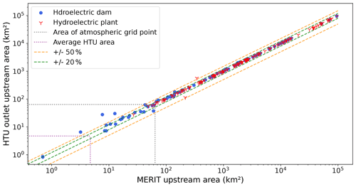
Figure 6 Comparison of the initial upstream area of the infrastructure (referenced in the database or upstream area of the MERIT pixel on which it is placed) with its final upstream area in the HTU graph. Blue dots represent hydroelectric reservoirs (reservoirs that have been associated with power plants during the adduction network building step), and red signs represent hydropower plants. Dashed green and orange lines delineate a respective error of ±20 % and ±50 %, while dotted gray and purple lines refer, respectively, to the area of an atmospheric grid point and the average area of an HTU.

3.3 Data for water demands and validation

3.3.1 Ecological and irrigation demands

In France, minimum flow requirements are defined relatively to the mean interannual flow downstream of the dam $\stackrel{\mathrm{‾}}{{\mathrm{Dis}}_i}$. They are summarized in Table 2. We ran a 20-year SAFRAN simulation without reservoir operations to calculate $\stackrel{\mathrm{‾}}{{\mathrm{Dis}}_i}$ at dam locations.

Table 2 French legal requirements for ecological flow, $\stackrel{\mathrm{‾}}{{\mathrm{Dis}}_i}$ is the mean interannual flow downstream of the dam.

To account for the irrigation purposes of some reservoirs, we increase the minimum flow requirement downstream of reservoirs intended for irrigation during the summer period (1 June to 30 September) by setting α_irri=8. This choice is based on information available from French reservoir concession contracts, which sometimes specify the volume of water reserved for irrigation. In the case of Serre-Ponçon, for example, the concession contract stipulates a reserve of 200×10⁶ m³, to be used for irrigation, between 1 July and 30 September. If we consider a constant withdrawal spanning 3 months, this corresponds to a 25 m³ s⁻¹ flow, which is 45 % of the 55 m³ s⁻¹ mean interannual flow at this location and thus 9 times larger than F_min, which is set to 5 %, as explained above.

3.3.2 Hydropower production demand

As this study aims to validate our proposed reservoir operations model, we take the historical time series of production as the hydropower demand prescribed to the model. We can thus assess whether the model, when driven by the historical atmospheric dataset, can meet the observed production levels. Data on observed production for hydropower plants in the French power grid are available from 2015 onwards, published by RTE, the French TSO, at a 30 min time step for two categories of plants (, ):

• river production D_river(t) that gathers the production of pure run-of-river power plants and poundage power plants (reservoir plants with a storage below 400 h)

• reservoir production D_res(t) that gathers the production of reservoir power plants with a greater storage capacity.

In our model, D_river(t) is then used to drive the production of run-of-river and poundage power plants, while D_res(t) is used for the reservoir power plants with greater storage capacity, both using the method described in Sect. 2.3.2. We use the classification established by RTE and illustrated in Fig. B2.

3.3.3 Validation data

In France, hydropower reservoirs are managed by companies that do not share detailed data on their production or their filling level. Similarly, discharge data from gauging stations near hydroelectric power plants are often not publicly accessible. This limits the data available for validating our model.

However, as a delegate of public services, RTE provides some data, often aggregated at the national level, which allows us to calibrate and validate our model as shown in the following two sections.

The available data are as follows:

• national time series of production by hydroelectric sector (river and reservoir) at 30 min time step from 2015 (, ) – which are the time series used for the hydropower production demand;

• annual production of each hydroelectric power plant for the years 2015, 2016, and 2018 (ODRÉ, 2015, 2016, 2018);

• weekly hydraulic stock (Eq. 17) at national level from 2014 to 2020 (, ).

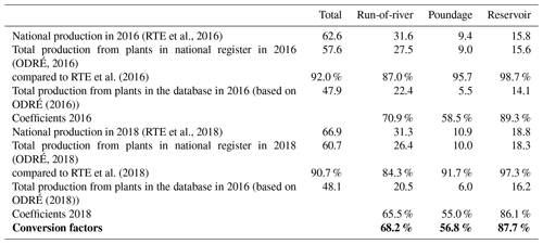
As mentioned in Appendix B, our hydropower plant dataset does not cover all the installed plants in France. However, using annual production data of each plant provided by ODRÉ (2015, 2016, 2018), we can estimate the share of the national production provided by the power plants in our database. This allows us to compute a factor for converting the production from national time series (, ) into representative production within our model, for both prescribing the production demand and comparing the results. The calculation of such conversion factors is presented in Table B2.

We also compute the maximum hydraulic stock of the reservoirs associated with the power plants in our database using Eq. (17) and data from our plants and reservoirs databases. We obtain S_max=3.66 TWh, which is quite close to the 3.59 TWh value reported by RTE (, ). Therefore, we can consider that our database covers all the available storage and that missing hydropower capacity is linked to negligible reservoirs.

4 Results

4.1 Calibration

Here we present the application of the calibration process to the French study case. First, we assess the discrepancies between the AHP simulated by the model (Eq. 16) and the observed annual production at each power plant for the years with available data. We then discuss the likely origin of these discrepancies. Finally, the calibration process is validated by comparing annual potentials simulated in ORCHIDEE to the observed annual production at the national level for an extended period, using data from 2000 to 2020. We choose to use SAFRAN forcing as a reference for the calibration step, as this dataset is widely used in regional studies of France.

4.1.1 Discrepancies between AHP and the historical production

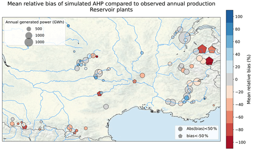
Figure 7 shows the average relative bias of simulated AHP compared to observed production for the 3 years with available data for the run-of-river plants in our database. For most plants, the bias in hydropower potential is comparable to the bias in river discharge computed at nearby stations, which is displayed in Fig. E1. This indicates that the bias mainly stems from hydro-meteorological errors (reason 1 of the list presented in Sect. 2.5). At the Caderousse and Gambsheim power plants, located in Fig. 7, a stronger positive bias is found. At these locations, only part of the river flows through the plant, which explains the computed bias (reason 3). The calibration leads to obtained efficiencies ranging from 0.43 to 1.31, with a median value of 0.88.

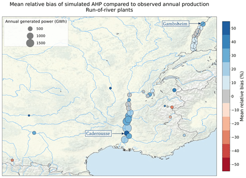
Figure 7 Average relative bias of simulated AHP compared to observed annual production for run-of-river power plants with available data. The point size corresponds to the average annual production. Source: authors, based on a layer by U.S. National Park Service.

Over a year, the water entering the reservoir of a reservoir or poundage power plant can either contribute to the annual production of the plant E_(i,j)(y), contribute to the annual change in the hydraulic stock within the reservoir ΔS_i(y), or spill without generating power. Observed production E_(i,j)(y) is available for the 3 years mentioned earlier. However, observations of changes in the hydraulic stock are only available at the national level, for the national stock $\mathrm{\Delta }{S}_{\mathrm{obs}}\left(y\right)={\sum }_{i\text{in res}}\mathrm{\Delta }{S}_i\left(y\right)$. To compare simulated AHPs with observations of production and stored energy, we make the two following assumptions: (i) spillages that do not produce power can be neglected, and (ii) the changes in the hydraulic stock are homogeneous across all reservoirs, $\forall i,\mathrm{\Delta }{S}_i\left(y\right)=\mathrm{\Delta }{S}_{obs}\left(y\right)\times \frac{S_{\max }}{S_{i,\max }}$. In Fig. 8, we plot the average bias of AHP_(i,j)(y) relative to observed net production $E_{(i,j)}\left(y\right)+\mathrm{\Delta }{S}_i\left(y\right)$ for the 3 years for which data are available. It enables us to distinguish two types of bias in the simulated AHP, suggesting that two main error sources can be distinguished:

• Plants with an absolute bias inferior to 50 % (represented by circles in Fig. 8). Their biases are generally similar to those of discharge for nearby stations, displayed in Fig. E1.

• Plants with a bias inferior to −50 % (represented by pentagons in Fig. 8). These plants are mainly located in mountainous areas and have a negative bias stronger than that of the discharges in the area. Moreover, their biases have a small interannual variance, indicating that the error is stable over time (not shown).

Figure 8 Average relative bias of simulated AHP compared to observed net annual production for reservoir and poundage power plants with available data. The point size corresponds to the average annual production. Source: authors, based on a layer by U.S. National Park Service.

4.1.2 Validation of the calibration

The performance of the calibrated model is assessed by comparing the potentials simulated by the calibrated model forced by SAFRAN with the historical annual production (, ) at the national scale over the whole period 2010–2020. For each plant category, the simulated annual potential is computed by summing the AHP of all plants within this category. For poundage and reservoir plants, we directly compare this aggregated potential to the historical production, as stock data (, ) are not available for the whole period. This relies on the assumption that the national stock returns to its initial value at the end of each year.

The calibration appears to be robust as very small biases (less than 3 %) are obtained when comparing the simulated potentials to the observed production (Fig. 9). The relative differences in annual production are on average lower than 10 %. This indicates that the model is able to capture the overall pattern of interannual variability of the observed production.

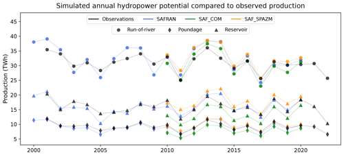
Figure 9 Comparison of estimated annual hydropower potential with observed annual production for the different categories of hydropower plants and for the different atmospheric forcings, after calibration based on SAFRAN.

We also explore the sensitivity of the model and calibration procedure to the uncertainties in precipitation forcings that are highlighted in Figs. C1 and E2. We compute AHPs under the two alternative forcings (Fig. 9) and compare the obtained inter-forcing variability with the inter-annual variability of observed production (Table 3). Run-of-river annual potentials exhibit little variation across the different forcings, as the simulated flows of major rivers hosting run-of-river power plants (primarily the Rhône and the Rhine) demonstrate a low sensitivity to precipitation uncertainty (see Fig. E3). Consequently, the inter-forcing variability of simulated potential is 3 times smaller than the interannual variability of run-of-river power production (see Table 3). It is also slightly smaller than the modeling error, indicating a low sensitivity of simulated run-of-river production to the precipitation uncertainty. Conversely, reservoir plant production shows a much higher sensitivity to precipitation disparities between forcings. Lower COMEPHORE precipitation in mountainous regions lead to an average decrease of 18.7 % in the total simulated potential, compared to the SAFRAN simulation. As a result, the variability among forcings is of the same order of magnitude as the interannual variability of production and is higher than the modeling error. Finally, poundage power plants fall in an intermediate category, displaying an inter-forcing variability that is 41 % lower than the interannual variability.

In conclusion, the uncertainties in precipitation forcing in mountainous regions prove to be critical in the estimation of realistic hydropower potentials for reservoir plants. The calibration carried out relative to SAFRAN is less effective for other forcings, SAF_COM for instance, as the differences in precipitation data appear as the main contributor to the differences in hydropower potentials.

Table 3 Estimation of the errors in annual potentials' prediction.

^a We define the interannual variability daily as the standard deviation of observed annual production. ^b We define the inter-forcing variability as the mean standard deviation of annual potential across the forcings. ^c We define the modeling error as the RMSE of SAFRAN-simulated potentials compared to observations.

4.2 Hydropower operations

In this section, we assess the model's ability to simulate reservoir management and hydropower production. Observed time series of river production (gathering run-of-river and poundage power plants) and reservoir production serve as demand inputs for the reservoir operations in the model. At each time step, the model aims to meet this target by operating the reservoirs according to the rules described in Sect. 2.3 and the simulated hydrological cycle. The objective is to verify if our model can simulate operations consistent with observed production. Here we present the results obtained from a simulation spanning the period from 2015 to 2020.

4.2.1 River production

At each time step, the model first computes the available potential from fatal production (from run-of-river plants and spilled or constrained releases from the reservoirs of poundage plants). If this potential falls short of fulfilling the production target, the model then operates the reservoirs connected with poundage plants to supplement the production.

Figure 10 details how the simulation compares to the prescribed production over the period when the model is forced by SAFRAN. The model successfully reproduces the overall seasonality of production, meeting the hourly production target 69.0 % of the time. The failures (in red in Fig. 10) account for 6.9 % of the total prescribed production across the 6 years. They mostly occur during summer and fall, indicating that the simulated hydrology is unable to produce what was actually produced during these periods. In winter and spring, conversely, there are instances when the potential of fatal production exceeds the target production (January and February 2018, for instance). This means that the model could have generated more power during these periods than was actually produced. These discrepancies are likely due to the seasonality bias in discharge within the Rhône and Rhine catchments, as highlighted in Fig. E4. Despite these discrepancies, the performance of the model remains satisfactory, as it captures the gross seasonality and magnitude of run-of-river production, in addition to the inter-annual variability (Fig. 9).

Figure 10 Daily production from run-of-river and poundage plants. The purple line indicates the production prescribed to the model, and the red coloring shows the failures of the model to meet this target production, when the model is forced by SAFRAN. The other colors refer to the nature of the flow that contributes to the simulated production. Light blue represents the gross potential of run-of-river plants; dark blue represents the potential from spill from poundage reservoir (water overflowing from the reservoir); green represents the potential from constrained releases from poundage reservoirs; and lastly orange represents the dispatchable production, generated by the water specifically released from the poundage reservoirs for power generation.

The run-of-river production simulated by the model when forced by the alternative forcings SAF_SPAZM and SAF_COM is presented in Figs. C2 and C4. Using SAF_SPAZM, the failures in meeting the prescribed production are reduced (4.3 % of production not satisfied compared to 6.9 %) due to slightly higher annual potentials of run-of-river and poundage power plants (Fig. 9). On the other hand, higher failures are obtained with SAF_COM (15.4 % of the total production), consistently with the lower potentials obtained in Fig. 9. However, the seasonality remains very similar in all three simulations, consistent with the similar seasonality of the simulated discharges for the Rhine and Rhône rivers (Fig. E2).

4.2.2 Reservoir production

Similarly, a 30 min time series of observed production by reservoir power plants is prescribed to the model. To fulfill this demand, the model first computes the non-dispatchable production, available from reservoir spillage and constrained releases, by operating reservoirs according to the rules defined in Sect. 2.3. Figure 11 details how the simulation compares to the prescribed production throughout the period when forced by SAFRAN. Simulated production under the other forcings is presented in Figs. C3 and C5. Figure 12 displays the co-evolution of the observed national hydraulic stock (, ) and the one simulated by the model (Eq. 17) with the three forcings under study.

Figure 11 Daily production from reservoir plants. The purple line indicates the production prescribed to the model. The other colors refer to the nature of the flow that contributes to the simulated production. Blue represents the gross potential from reservoir spillage (water overflowing from the reservoir); green represents the potential from constrained releases from the reservoirs; and lastly orange represents the dispatchable production, generated by the water specifically released for power generation.

Figure 12 Comparison of simulated and observed national hydraulic stock evolution.

Under SAFRAN, the model successfully meets the production target while simulating hydraulic stock variations consistent with observations throughout the 6-year period. Reservoirs are filled during the spring due to snowmelt and depleted during the winter to meet the high electricity demand. Nevertheless, a slight temporal shift is observed, as the simulated stock starts to fill some weeks earlier compared to the observations. This temporal shift aligns with the seasonal biases in river discharges identified at the Chamonix station (Fig. E4), indicating a consistent pattern.

Under SAF_SPAZM, the stock remains significantly higher than the observations. Indeed, the simulated annual potential of reservoir power plants exceeds their observed production (Fig. 9), resulting in reduced releases from the reservoirs to meet the prescribed demand. This leads to high levels of unused spillage, as shown in Fig. C3.

Under SAF_COM, however, the stock is completely depleted after the first 2 years of simulation, and a significant portion of the demand cannot be satisfied (Fig. C5). This is consistent with the huge difference in annual production estimates highlighted in Fig. 9. In addition to the substantial deficit in hydropower potential, a negative feedback loop comes into play. As the reservoir storage diminishes, the head of the power plants decreases, reducing the power generation for a given released volume. Consequently, more water is drawn to generate the same amount of energy, further exacerbating the decline in reservoir storage. The calibration carried out relative to SAFRAN is not effective in avoiding this outcome.

Figure 11 allows for the distinction of the different drivers of French hydropower production, depending on the season. In winter, hydropower production is substantial, driven primarily by high electricity demand. Most of the production stems from intentional reservoir operations, with a minimal portion attributed to fatal production. In spring, fatal production becomes more prominent, particularly due to snowmelt-induced spillage, resulting in a minimum hourly production, even during periods of low power demand, such as at night (only visible at the hourly resolution not displayed here). During summer, a significant portion of the hydropower potential comes from constrained ecological and agricultural water releases. When looking at the hourly production (not displayed here), we find a good agreement between the simulated minimum production and the observed troughs in RTE's production.

4.3 Effects of hydropower operations on river discharges

We explore in this section the extent to which the representation of hydropower operations can reduce the hydro-meteorological errors of the model discussed in Appendix E, using the example of two gauging stations located in the Alps. Figure 13 details the location of these stations compared to the hydropower network. The Aiguebelle station is located on the Arc River, just upstream of its confluence with the Isère River and downstream from a series of hydropower plants, including one that generates electricity through the releases from a dam on the Isère River. The Cheylas station is located on the Isère River, downstream of its confluence with the Arc.

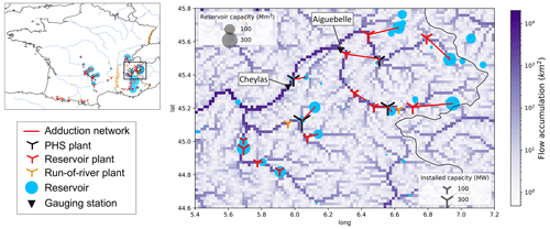
Figure 13 Location of Aiguebelle and Cheylas stations compared to hydropower infrastructures in the Arc catchment (French Alps). PSH plants are pumped storage hydropower plants not considered in this study.

Figure 14 compares the seasonality of the discharges simulated at these two locations by ORCHIDEE forced by SAFRAN with and without activating the hydropower operations module.

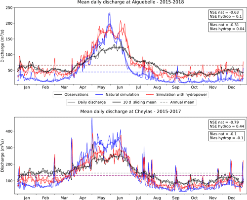
Figure 14 Comparison of daily (fine line) simulated river discharge with hydropower operations (red) and without (blue) and observed discharge (black) for two gauging stations in the French Alps. The thicker line is the 10 d average, while the dashed line is the annual mean.

At the Aiguebelle station, implementing hydropower operations significantly reduces the annual bias from −31 % to −4 % (Fig. 14). Indeed, when hydropower operations are activated, a portion of the Isère's water is diverted from its natural outlet to supply a power plant on the Arc. At Cheylas, no change is observed in the bias of the simulated river discharge. Furthermore, the seasonality of discharge is improved at both stations, with higher flows in fall and winter due to releases for power generation. This results in a significant improvement in the Nash–Sutcliffe efficiency (NSE) metric.

We found a similar effect for other French watersheds where flow observations near hydropower plants are available. However, as mentioned earlier, the confidentiality surrounding French hydroelectric production complicates a systematic and precise evaluation of this improvement in flow simulation.

5 Discussion and conclusion

5.1 A demand-based approach

This study demonstrated the effectiveness of a demand-based approach to simulate hydropower operations in land surface models. The conceptual framework of this approach was first described, emphasizing its three original features: (i) the reconstruction of the human-made hydropower network within the model grid to represent not only natural water flows but also those built for hydropower management; (ii) the implementation of reservoir operation rules that account for their multipurpose objectives; and (iii) the prescription of an exogenous “hydropower demand” defined at the power grid level to drive the release rules of hydroelectric reservoirs, allowing the coordinated management of all hydroelectric resources on the power grid in line with power system needs. Subsequently, we assessed the performance of this approach when implemented in the routing module of the ORCHIDEE model, for the case study of the French power grid. The ORCHIDEE model was run driven by an atmospheric reanalysis dataset, and national historic hydropower production time series were prescribed to the model as the hydropower demand to satisfy. The results indicate that when the model is forced to reproduce the historic generation, the implemented method simulates hydroelectric reservoir operations in line with the observations of reservoir storage at the national level.

Beyond this satisfactory result, our method presents several limitations and opportunities for improvement.

First, the time series used to drive the reservoir releases in this study is the actual production of dispatchable hydropower plants, which may differ from the real demand for dispatchable hydropower production. Indeed, the actual production is the result of a trade-off between the demand and the prevailing hydrological conditions, particularly the storage level in reservoirs. If this storage is low, the demand might not be fully satisfied to preserve water for future needs. In addition, we consider an exogenous dispatch of the hydropower production across the different types of hydropower plants (namely run-of-river and reservoir) at each time step. This approach facilitates the identification of model deficiencies for each type of power plant. For instance, we found a seasonal bias in run-of-river hydropower production, which would have been overlooked if a single production target had been used for all power plants. The reservoir plants would have served as buffers, reducing their production during periods of excess run-of-river output and increasing it during periods of deficits, thereby resulting in discrepancies in the stock evolution. However, in reality, the dispatch of power demand across the different types of hydropower plants is not exogenous but also depends on the hydrological conditions, as the potential for run-of-river production is fully exploited before turning to dispatchable units. To capture these intricate interactions between hydrology and hydropower production decisions, a solution is to couple our model with an economic power system dispatch model (Oikonomou et al., 2022). This coupling would ensure that the power demand dispatch used to drive reservoir operations in ORCHIDEE considers the hydrological conditions simulated within the model. This would result in a comprehensive modeling framework wherein simulated hydropower production simultaneously adheres to constraints related to water availability, non-power reservoir operations, and minimization of power system costs. In particular, hydropower demand would be endogenously adjusted to match the hydropower potentials of the simulated hydrology and could avoid entering the feedback loop where reservoirs are emptied, as in the SAF_COM simulation. This novel approach holds significant promises for enhancing the consistency and realism of hydropower production simulations, in particular to study the joint impacts of climate change and variable renewable energy integration.

Second, in this study, we opted for a simple rule to distribute national production among the power plants and demonstrated that such a rule could simulate credible hydroelectric operations at the national level. Since no time series of production data is available for individual plants in France, the realism of the simulated operations at the granular level cannot be assessed. However, the choice of the distribution rule could be further investigated, in particular by testing alternative rules, such as those proposed by Lund and Guzman (1999). Additionally, the operations we simulate assume that a social planner controls the entire grid's power plants and reservoirs, optimizing the collective production. In reality, power plants may belong to different stakeholders, each seeking to maximize their profit. Ambec and Doucet (2003) have shown that such decentralized management can lead to suboptimal resource management, which could not be reproduced by the proposed model. However, in the case of France, our assumption is justified as the historical production company, EDF, owns nearly 85 % of the hydroelectric production.

Third, as we focused primarily on hydroelectric usage, other water uses are simplified or even omitted in the current version of the model. Specifically, no water abstraction for domestic, industrial, or agricultural needs is included. Following Zhou et al. (2021), the irrigation demand could be explicitly calculated by the model based on the deficit between potential and actual evapotranspiration. In other studies, domestic and industrial water demands are estimated using socio-economic proxies such as population density or GDP (Neverre, 2015).

5.2 Sources of uncertainties

We have paid particular attention to identifying and discriminating among the various sources of uncertainty that may affect the estimation of hydroelectric production using such a method. Our findings indicate that while errors in simulated discharge are prevalent in most watersheds in our case study, the limited knowledge of the hydroelectric adduction network is the main source of uncertainty for hydropower infrastructures in mountainous basins. To our knowledge, no dataset comprehensively documents these complex “hydroelectric links”, which operate on a small scale. Therefore, an in-depth analysis of the gray literature released by the various stakeholders is necessary to reconstruct this network in detail. Furthermore, we proposed a calibration method to overcome this limitation and validated it against observations for the case study of France. This method can therefore be extended to countries with limited information available on the hydroelectric network.

Regarding hydro-meteorological errors, the use of three different precipitation datasets allows us to understand their more precise origin. In several watersheds crucial for hydroelectricity (such as Durance or Lot), and especially in the upstream parts, uncertainties in observed precipitation appear to be the primary contributor to the error in simulated discharge. On the Rhône or the Rhine rivers, conversely, errors in the simulated discharges seem to stem more from processes not represented in the model, such as water withdrawals for human uses. Though incomplete, this work contributes to the current effort to integrate human water management into hydrological models, in order to simulate a more realistic water cycle (Nazemi and Wheater, 2015a). We show that our method can improve river flow simulations in some mountain catchments where hydropower cannot be neglected.

Finally, our study shows that comparing hydropower estimates with observed production offers an indirect means of assessing the quality of meteorological data. In our study case, we demonstrated the lower quality of the COMEPHORE dataset in mountainous regions compared to SAFRAN or SPAZM, something already identified by Birman et al. (2017) and Magand et al. (2018).

5.3 Perspectives

In conclusion, the demand-based operations proposed in this study hold promising prospects for enhancing our understanding of the resilience of different power mix scenarios to changes in climate, water management, or land use. The next steps in this trajectory involve (i) integrating our climate-based hydropower model with a power system model to get a comprehensive framework that captures all relevant constraints on hydropower production, (ii) applying this integrated framework to climate change scenarios and power system scenarios to evaluate the adaptive capacity of the power grids, and (iii) refining the description of other water uses to more completely describe the competition for water resources.

Such a detailed model could also be instrumental in planning future hydropower expansion more sustainably. It would help assess the demand satisfied by new hydropower plants at the grid scale, considering both existing and planned hydropower plants. Besides, the model could evaluate the potential impacts of new projects on river discharges and ecosystems.

Appendix A: Building the routing network

A1 Locating hydroelectric infrastructures on the river network

Dams and hydropower plants are located on the MERIT grid based on georeferenced and upstream area information provided in the databases. The infrastructure datasets used for the France case study are presented in Appendix B. The location procedure is done following these steps:

1. The initial location is identified based on geographical coordinates.

2. A search area is defined around this initial location (typically with a 10 km in radius).

   • If the upstream area of the infrastructure is available in the databases, we identify all the pixels in the search area that have an upstream area close to the referenced one (typically ±20 %). Among these eligible pixels, the one closest to the initial location is selected. If no pixel meets the criteria, the infrastructure is not placed.

   • If no upstream area data are available in the databases, we look for the closest pixel to the initial location that is likely to be situated on a river. To do this, the maximum upstream area of the pixels in the search area is identified (U_max), and the closest pixel to the initial location satisfying the condition $U>\frac{U_{\max }}{\mathrm{10}}$ is selected, where U is the upstream area of the pixel.

Note that each vertex and edge can respectively contain only one dam and hydropower plant. If several dams are placed on the same HTU during pixel aggregation, their respective reservoir volumes for the different uses are summed. If two plants are placed on the same edge, their installed power capacity and head are only summed if both plants have the same input point. Otherwise, only the plant with the highest installed capacity is kept. As in other studies (Abeshu et al., 2023), all the reservoir attributes are associated with the HTU of the dam (even if its water surface can be larger than the HTU area and its geometry is different from the HTU geometry).

A2 Adduction network

Poundage and reservoir plants generate electricity from the water released from upper reservoirs. To explicitly represent this adduction network in our model, we need to identify such connections between a feeding reservoir and a power plant. Since datasets describing these connections are rarely available, we use an algorithm to identify them. For each poundage or reservoir plant, we select as the feeding reservoir the one that maximizes the potential function $\mathit{\varphi }=\frac{U\cdot V\cdot h}{d}$, where U is the upstream area of the dam, V is the storage capacity of the reservoir, h is the elevation difference between the plant and the dam, and d is the horizontal distance between them. The definition of this potential function is inspired by similar approaches aiming to connect an irrigated area to a water supply point (Neverre, 2015; Zhou et al., 2021).

This position algorithm relies on the assumption that each plant is fed by only one reservoir. This assumption is however debatable, especially for plants in mountainous regions, which may be connected to several reservoirs. In this case, the potential function ϕ privileges the reservoir with the largest upstream area, as it is likely to have the most significant influence on the plant's production potential. During calibration (see Sect. 2.5), plants for which the identification of a single reservoir conducts a significant misrepresentation of the plant's production potential are identified, and a correction is made by moving the withdrawal point so that it gathers enough water to ensure the observed production is possible.

Appendix B: Datasets

B1 Dams and reservoirs

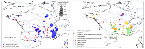
We use reservoir data from the GRanD (Global Reservoir and Dam Database) (Lehner et al., 2011), which compiles data on large reservoirs and dams worldwide (volume > 0.1 km³, totaling 7320 dams). The database includes 137 dams in France, 63 of which are used for hydroelectricity. However, some important dams for French hydroelectricity are not documented in this database. Therefore we completed the dataset with data from the CFBR (Comité Français des Barrages et des Réservoirs), responsible for the inventory of French dams higher than 15 m for the ICOLD (International Commission on Large Dams). We extracted data from its website (CFBR, 2021) to complete the GRanD database. Our final dataset comprises 492 French dams. Their location, original data sources, and intended purposes are shown in Fig. B1.

Figure B1 Location and main uses of the reservoirs in the final database.

B2 Hydropower plants

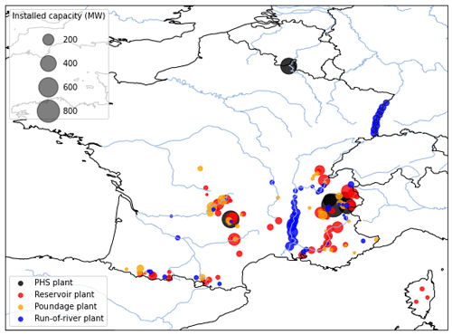
The data used in this study are obtained from the European Commission and Joint Research Centre (2019) database. This database includes geographical coordinates, installed power capacity, plant type (run-of-river, reservoir, or pumped storage hydropower (PSH)), and hydraulic head information for 4186 European plants, totaling an installed capacity of 161 GW. Of these, 153 plants are located in France, representing 20.6 GW of capacity. Other available datasets of French hydropower plants are the national registers of electricity generation and storage facilities published annually (ODRÉ, 2016, 2018). The 2016 register includes data on 414 hydropower plants, with a total installed capacity of 23.4 GW. However, as these registers do not provide the geographical coordinates of the plants, we chose to use the JRC database. Nevertheless, we use data from the 2016 national register to correct head information and categorize the plants according to the four categories used by the French operator: run-of-river, poundage, reservoir, and PSH. Figure B2 shows the locations of the plants included in our final database, while Table B1 summarizes the discrepancies between the databases in terms of installed capacities.

(ODRÉ, 2016)ODRÉ (2016)

Table B1 Comparison of the different databases in terms of installed hydroelectric capacities (GW) in metropolitan France (without Corsica and overseas territories).

Figure B2 Typology of the plants in the database.

B3 Conversion factors for hydropower generation

As presented in Table B1, our final dataset does not include all the hydropower plants installed in France. However, using annual production data of each plant provided by ODRÉ (2015, 2016, 2018), we can estimate the share of the national production accounted for by the plants included in our database. This allows us to compute a factor to convert the actual production of national time series (, ) into representative production in our model, for both prescribing the production demand and comparing the results. The computation of such conversion factors is presented in Table B2. It relies on the assumption that within each category of power plant, the geographical distribution of plants in our database is representative of all French power plants; therefore production ratios remain constant over time. This assumption is debatable as our database primarily includes the largest power plants in terms of installed capacity, which are often concentrated in certain regions, while smaller plants may be located in watersheds not represented in our database (e.g., run-of-river plants on the Seine River). However, as the missing plants have, by definition, a lower installed capacity than those in our database, their contribution to national production is lower and can reasonably be neglected.

(RTE et al., 2016)(ODRÉ, 2016)RTE et al. (2016)ODRÉ (2016)(RTE et al., 2018)(ODRÉ, 2018)RTE et al. (2018)ODRÉ (2018)

Table B2 Comparison of the different available databases in terms of annual production (TWh) and calculation of conversion factors. Bold font emphasizes the importance of the conversion factors.

Appendix C: Alternative precipitation datasets

C1 Dataset presentation

C1.1 COMEPHORE

The COMEPHORE (COmbinaison en vue de la Meilleure Estimation de la Précipitation HOraiRE) dataset provides observations of surface precipitation accumulation over metropolitan France at an hourly and kilometric resolution based on a synthesis of radar and rain gauge data. A specific processing chain has been implemented in order to address the various sources of error affecting radar data, in particular its low quality in high-altitude mountainous areas like the Alps or the Pyrenees (Fumière et al., 2020). The final database is nevertheless assumed to be the best representation of surface precipitation over metropolitan France (Fumière et al., 2020).

We build a meteorologic dataset SAF_COM by replacing precipitation data in SAFRAN with data from COMEPHORE. As COMEPHORE does not distinguish solid and liquid precipitation, we keep SAFRAN's hourly ratio of solid to liquid precipitation when possible and discriminate based on the air temperature otherwise.

The differences in annual mean precipitation between SAFRAN and COMEPHORE are generally small, with an average deviation inferior to 1.0 % (Fig. C1). However, we find a small seasonal bias as this average deviation ranges from −2.0 % in winter to +1.9 % in summer. Moreover, discrepancies increase dramatically in mountainous regions, especially in the Alps and the Pyrenees. For grid points with an average elevation above 1000 m, the annual mean precipitation in COMEPHORE is, on average, 10.4 % lower than in SAFRAN.

C1.2 SPAZM

SPAZM (SPAtialisation des précipitations en Zone de Montagne) is a daily reanalysis of precipitation at the kilometer scale, developed by EDF, France's main electricity producer. SPAZM specifically covers the southern half of the French territory, where a large majority of hydroelectric power plants are located (Gottardi et al., 2008). Climatological precipitation outlines are first constructed based on daily precipitation observations categorized by types of oceanic circulation (weather patterns). These outlines are then spatially interpolated onto the kilometer-scale grid and deformed daily according to available observations. In addition to Météo-France's observations, which are also used to construct SAFRAN, EDF's measurement network is utilized. We interpolate the daily precipitation data from SPAZM to the hourly scale and merge them with SAFRAN data to create the alternative forcing dataset SAF_SPAZM. As for SAF_COM, we keep SAFRAN's hourly ratio of solid to liquid precipitation when possible. Compared to SAFRAN, SPAZM's precipitation is on average 2.7 % higher, with a bias of +7.0 % in summer and +2.1 % in winter. The bias is heterogeneously spread over France (Fig. C1), with larger differences in the highest reliefs, without a clear sign. For grid points above 1000 m, the average deviation is +3.9 %.

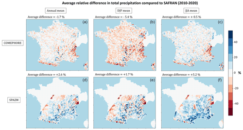
Figure C1 Relative differences in total precipitation across the datasets for the period 2010–2020. (a, d) Annual average difference, (b, e) average difference in winter (December–January–February), and (c, f) average difference in summer (June–July–August). (a–c) COMEPHORE dataset compared to SAFRAN and (d–f) SPAZM compared to SAFRAN.

C2 Simulation of hydropower production under SAF_SPAZM

Figure C2 Daily production from run-of-river and poundage plants simulated in the model when forced by SAF_SPAZM. The purple line indicates the production prescribed to the model, and the red coloring shows the failures of the model to meet this target production. The other colors refer to the nature of the flow that contributes to the simulated production. Light blue represents the gross potential of run-of-river plants; dark blue represents the potential from spillage from poundage reservoirs (water overflowing from the reservoir); green represents the potential from constrained releases of poundage reservoirs; and lastly orange represents the dispatchable production, generated by the water specifically released from the poundage reservoirs for power generation.

Figure C3 Daily production from reservoir plants simulated in the model when forced by SAF_SPAZM. The purple line indicates the production that has been prescribed to the model. The other colors refer to the nature of the flow that contributes to the simulated production. Blue represents the gross potential from reservoir spillage (water overflowing from the reservoir); green represents the potential from constrained releases from the reservoirs; and lastly orange represents the dispatchable production, generated by the water specifically released for power generation.

C3 Simulation of hydropower production under SAF_COM

Figure C4 Daily production from run-of-river and poundage plants simulated in the model when forced by SAF_COM. The purple line indicates the production prescribed to the model, and the red coloring shows the failures of the model to meet this target production. The other colors refer to the nature of the flow that contributes to the simulated production. Light blue represents the gross potential of run-of-river plants; dark blue represents the potential from spillage from poundage reservoirs (water overflowing from the reservoir); green represents the potential from constrained releases of poundage reservoirs; and lastly orange represents the dispatchable production, generated by the water specifically released from the poundage reservoirs for power generation.

Figure C5 Daily production from reservoir plants simulated in the model when forced by SAF_COM. The purple line indicates the production that has been prescribed to the model. The other colors refer to the nature of the flow that contributes to the simulated production. Blue represents the gross potential from reservoir spillage (water overflowing from the reservoir); green represents the potential from constrained releases from the reservoirs; and lastly orange represents the dispatchable production, generated by the water specifically released for power generation.

Appendix D: Hydropower network error

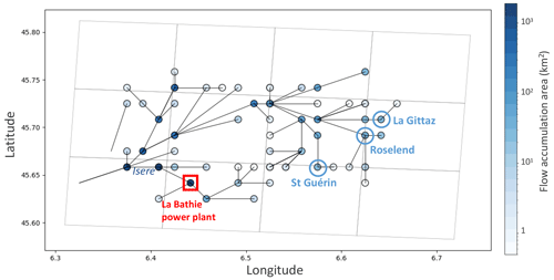
The La Bâthie power plant is the most important reservoir hydropower plant in France in terms of installed capacity. It is located in the Alps and is fed by numerous water intakes, as illustrated in Fig. D1. These include the reservoirs of Roselend, Saint Guérin, and La Gittaz, as well as other intakes directly connected to rivers or glaciers.

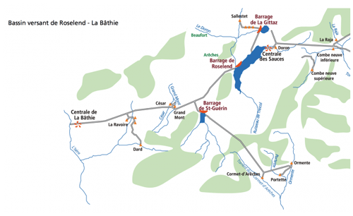
Figure D1 Schematic representation of the water adduction network to La Bâthie power plant (source: https://vpah-auvergne-rhone-alpes.fr/, last access: 11 November 2024)

Figure D2 describes the same area in HTUs' space and shows that the Roselend reservoir accounts for only a small part of the water being transferred to the hydropower plant.

Figure D2 HTUs' representation in the model for the same spatial area as Figure D1. The location of hydropower infrastructures is indicated.

Appendix E: Hydro-meteorological errors

To evaluate the performance of the ORCHIDEE model in simulating river discharges in France, independent of reservoir operations, we compare the daily river discharges simulated by the model with observations from Schapi (2022) database. It is important to note that the observed discharge data represent actual discharge values, including water withdrawals, while, at this stage, ORCHIDEE generates natural discharges without accounting for such withdrawals and dam operations.

E1 Bias in average discharge

Figure E1 displays the relative biases in the mean discharge simulated by ORCHIDEE forced by SAFRAN over the 2010–2020 period for a selection of gauging stations located on rivers with hydropower infrastructure (see Fig. B2 for the detailed locations of the power plants). We chose the bias metric because the annual mean discharge is the most relevant parameter for hydropower potential.

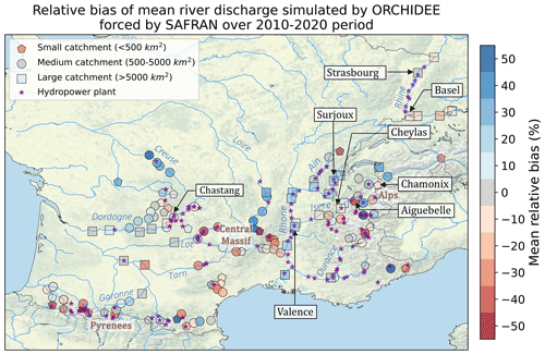
Figure E1 Relative bias in mean discharge for a selection of gauging stations located on French rivers equipped for hydropower, for the period 2010–2020. Each colored point represents a gauging station, with the shape indicating the size of its catchment, while the color indicates the discharge bias at this location. Purple stars indicate the locations of the hydropower plants located on the model grid. Source: authors, based on a layer by U.S. National Park Service.

The overall performance of the model indicates a slight overestimation of flows, with an average bias of +2.4 %. The discharge bias increases with the upstream area of stations. For small catchments (less than 500 km²), the average bias is −1.6 %. In medium-sized catchments (between 500 and 5000 km²), the bias is +1.1 %. In large catchments (more than 5000 km²), the bias becomes more pronounced, reaching +7.6 %. It is, however, important to note that the smaller the upstream area, the greater the uncertainty in the location of the station. In Fig. E1, only the stations located with an error in the upstream area lower than 20 % are displayed.

On the largest rivers (Rhine and Rhône), where most run-of-river power plants are located, the bias shows little spatial variability, remaining around +20 % for the Rhône and −10 % for the Rhine. In contrast, in the Alps, which has a significant share of the dispatchable hydroelectric capacity, the bias is highly variable, even within the same river. For instance, upstream of the Isère River, the bias varies from −19 % to +26 % between two stations located about 20 km apart. The upstream reaches of the Durance also show negative biases. In the other massifs equipped for hydroelectricity, such as the Pyrenees and Massif Central, there are negative biases at higher altitudes, which gradually diminish downstream.

Assuming negligible observational errors, discharge bias can originate from several error sources:

• errors in the atmospheric forcing applied to ORCHIDEE;

• modeling errors in the representation of energy, water, and carbon cycles;

• missing processes in ORCHIDEE, such as glacier melting, interactions with groundwater, and water withdrawals.

To explore the first hypothesis, Fig. E2 compares the discharges simulated by ORCHIDEE using the two alternative forcings (SAF_COM and SAF_SPAZM) with those from the reference SAFRAN simulation. The relative biases of these simulations compared to observations are presented in Fig. E3.

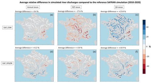
Figure E2 Relative difference in discharge simulated by ORCHIDEE under the alternative precipitation forcings. Results are expressed as average relative differences compared to the reference SAFRAN simulation for the period 2010–2020. (a, d) Annual average difference, (b, e) average difference in winter (December–January–February), and (c, f) average difference in summer (June–July–August). The discharges are shown for all grid points with an upstream area greater than 1000 km².

Under the SAF_COM forcing, simulated discharges show relatively small differences from those obtained with SAFRAN on an annual average, except in mountainous watersheds (Alps and Pyrenees). In these regions, the lower precipitation in SAF_COM results in streamflows that are 30 % to 40 % lower when compared to the SAFRAN simulation. Besides, a pronounced seasonal pattern is observed. The simulated streamflows are lower in winter under SAF_COM across France (averaging −16 % and up to −50 % for the Loire and Durance rivers), while they are higher in summer (averaging +25 % and up to +50 % for the Loire River). Regarding the comparison with observed flows (Fig. E3, the negative biases observed with SAFRAN in the Alps and Pyrenees are accentuated under SAF_COM, particularly along the Durance and Isère rivers, where many hydroelectric power plants are located. However, for some Alpine stations and the Massif Central, where the flow is overestimated with SAFRAN, the flow is more accurately simulated under SAF_COM.

Under the SAF_SPAZM forcing, mean river discharges generally increase in most watersheds compared to the SAFRAN simulation, consistent with the higher precipitation in this dataset. However, the upper Rhône watershed stands out with a decrease in simulated discharge, reaching up to −40 % during the summer season, allowing for a reduction in the bias in simulated discharge in this area.

This analysis shows that variability in forcing data significantly influences simulated discharges, even if we limit our analysis to the precipitation variable without considering other forcing variables.

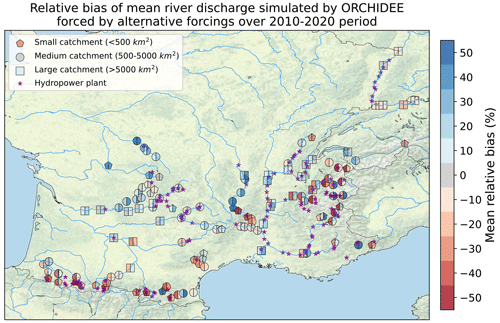
Figure E3 Relative bias in mean discharge simulated by ORCHIDEE under the alternative forcings for a selection of gauging stations located on French rivers equipped for hydropower, for the period 2010–2020. The left-hand coloring in the symbols indicates the discharge bias under SAF_COM, while the right-hand coloring indicates the discharge bias under SAF_SPAZM. Source: authors, based on a layer by U.S. National Park Service.

E2 Discharge seasonality

Beyond the bias in mean values, the performance of ORCHIDEE in reproducing the seasonality of the discharge is key for the modeling of run-of-river production as well as that of poundage power plants, which have very limited storage capacity. Observations and simulations of daily discharges under the SAFRAN forcing are presented in Fig. E4 for selected gauging stations in catchments equipped with run-of-river or poundage power plants.

As depicted in Fig. B2, run-of-river plants are mostly located along the Rhône and Rhine rivers. In the upper Rhône (Surjoux station), there is a substantial overestimation of high flows and an underestimation of low flows. The error reduces progressively downstream: the Nash–Sutcliffe efficiency (NSE) is better at the Valence station, despite a higher overall annual bias (likely due to the non-representation of water withdrawals). On the Rhine (Basel and Strasbourg stations), we see similar errors, with an underestimation of low flows during fall and an underestimation of the spring maximum. The discrepancy in the Rhône's seasonality can be attributed to the non-representation of Leman reservoir management in our model, which is known to play a crucial role in shaping discharge seasonality in the upper Rhône (Habets et al., 1999).

Poundage plants are distributed across various catchments. Some of them are concentrated in the upper Dordogne river, notably the Chastang plant, the most powerful poundage facility, which benefits from a gauging station at its location. We find a positive NSE for this station, indicating that the seasonality is well captured by the model.

Finally, some run-of-river and poundage plants are also concentrated in the Alps, where we focus on two gauging stations: Chamonix, situated in a small upper catchment, close to a run-of-river plant, and Cheylas, positioned on a large river (l'Isère), downstream from several power plants. At Chamonix, we find a seasonal bias as the model simulates an earlier discharge peak compared to observations (around 2 months ahead). At Cheylas, the model overestimates the seasonal variability of the discharge, with higher flows during spring and lower flows during winter, which can be attributed – at least in part – to the non-representation of reservoir management at this stage of our study (see Sect. 4.3).

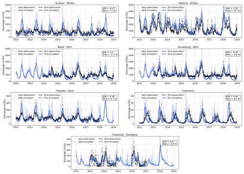
Figure E4 Comparison of simulated and observed river discharges for a selection of gauging stations. Locations of selected stations are indicated in Fig. E1. Fine lines and dots are daily time series, while thicker lines are 30 d sliding averages. NSE metrics are computed on a daily time series.