Seasonal variation in land cover estimates reveals sensitivities and opportunities for environmental models

Most readily available land use/land cover (LULC) data are developed using growing season remote sensing images often at annual time steps, but seasonal changes in remote sensing data can lead to inconsistencies in LULC classification, which could impact geospatial models based on LULC. We used the Dynamic World near-real-time global LULC dataset to compare how geospatial environmental models of water quality and hydrology respond to LULC estimated from growing vs. non-growing season data for temperate watersheds of the eastern United States. Non-growing season data resulted in LULC classifications that had more built area and less tree cover than growing season data due to seasonal impacts on classifications rather than actual LULC changes (e.g., quick construction or succession). In mixed-LULC watersheds, seasonal LULC classification inconsistencies could lead to differences in model outputs depending on the LULC season used, such as differences in watershed nitrogen yields simulated by the Soil and Water Assessment Tool. Within reason, using separate calibration for each season may compensate for these inconsistencies but lead to different model parameter optimizations. Our findings provide guidelines on the use of near-real-time and high-temporal-resolution LULC in geospatial models.

1 Introduction

Environmental models incorporating land use/land cover (LULC) data are common in many fields including hydrology, biogeochemistry, ecology, and climate science, often with decision-making implications (Hu et al., 2021; Baumgartner and Robinson, 2017; Naha et al., 2021; Li et al., 2021). Studies relating hydrology and water quality to LULC often use an LULC dataset developed primarily from growing season data, such as the United States National Land Cover Database (NLCD; Jin et al., 2019) or Cropland Data Layer (CDL; Boryan et al., 2011), and/or use an LULC dataset available at an annual time step (Sulla-Menashe and Friedl, 2018; Buchhorn et al., 2020; Gray et al., 2022). Characteristics of LULC (e.g., canopy density and precipitation interception) vary seasonally, particularly in temperate regions where vegetation leaf cover is reduced during the non-growing season compared to the growing season (van Beusekom et al., 2014). This has prompted popular hydrological models such as the Soil and Water Assessment Tool (SWAT; Arnold et al., 1998) to include seasonal cycles for factors like leaf area and crops (Nkwasa et al., 2020; Frans et al., 2013). However, there can also be temporal inconsistencies in LULC classifications due to variation in spectral signals that are often not accounted for, such as built LULC being classified as other types within the course of a year or other classes being classified as trees too quickly for natural succession (Cai et al., 2014; Gómez et al., 2016). Addressing temporal inconsistencies is important for accurately identifying LULC change (Sexton et al., 2013; Liu and Cai, 2012; Hermosilla et al., 2018), and various approaches have been developed that include incorporating time as a co-dependent in the classifier to remove illogical changes (Graesser et al., 2022) and probability-based statistics to separate noise from trends (Zhu et al., 2012; Zhu and Woodcock, 2014; Sulla-Menashe et al., 2019; Zhao et al., 2019). However, these approaches are typically not readily incorporated into watershed-scale hydrologic and water quality model frameworks, which take pre-classified LULC as model input (Li et al., 2019). These models are known to be sensitive to actual LULC changes over longer (e.g., >10-year) time spans, such as forests being converted to other LULC types (Li et al., 2019; Basu et al., 2022).

Present-day high-temporal-resolution LULC datasets, such as the global Dynamic World dataset (Brown et al., 2022), can facilitate the study of non-growing season and near-real-time impacts of LULC classifications on environmental models, including those of hydrology and water quality. Dynamic World, which has a 10 m spatial resolution at 5 d intervals from Sentinel-2 satellites (2A and 2B), has classification accuracy comparable to other LULC datasets including the NLCD, European Space Agency WorldCover, and Esri Land Cover data (Venter et al., 2022; Brown et al., 2022), and its 5 d temporal resolution is much more frequent than the annual-or-longer frequency of other common LULC datasets. This high spatiotemporal resolution creates unprecedented opportunities for modelers to study the impacts of phenomena such as emerging settlements, agricultural dynamics, and forest conversion on outputs such as ecosystem dynamics and biogeochemical budgets (Brown et al., 2022). For environmental research to take advantage of these high-temporal-resolution data, we need to understand the impacts of potential seasonal variation in LULC estimates on geospatial models, which use LULC data to support water resource management across the globe (Fu et al., 2019; Guo et al., 2020; Murphy, 2020). Evaluation of LULC products at high spatiotemporal resolution is an important research need with vast societal implications (Radeloff et al., 2024).

Worldwide, investigations of LULC impacts on hydrology and water quality often employ regression-based models (Fu et al., 2019; Dow and Zampella, 2000), SWAT models simulating LULC change (Ni et al., 2021; Tong et al., 2009), and/or SWAT model configurations compared objectively to evaluate model performance (Fuka et al., 2012; Li et al., 2019). We used the Dynamic World LULC dataset to demonstrate how estimates of LULC can change between the growing and non-growing seasons (note that estimates of LULC could change due to real transitions or due to illogical classification inconsistencies described above). We then used a long-term United States National Park Service (NPS) water quality dataset for temperate watersheds in the eastern United States, along with the above hydrologic and water quality models, to assess the use of seasonally based LULC classifications as an input for three modeling cases ranging from low to high complexity. We asked the following questions: how different are model outputs (effect sizes) when using growing vs. non-growing season LULC inputs, and are there differences in calibrated model performance if growing vs. non-growing season LULC input is used? We hypothesized that watersheds with mixed land cover types (e.g., a combination of built and trees) would have the greatest variability in land cover classification between growing and non-growing seasons due to heightened temporal inconsistencies, which could carry over into sensitivities for watershed-scale geospatial models.

2 Materials and methods

2.1 Study area and data

Our study area was 37 current (plus 18 historic) wadeable stream water quality sites monitored by the National Park Service National Capital Region Network (NCRN), with sites in Maryland; Virginia; West Virginia; and Washington, DC, USA (case no. 1; Fig. 1). All sites are in the Chesapeake Bay watershed and were chosen to help inform natural resource management (Norris et al., 2011). This includes the 167 km² Rock Creek watershed of Rock Creek Park (case no. 2) and the 150 km² Difficult Run watershed of George Washington Memorial Parkway (case no. 3), selected from the above watersheds for having continuous calibration and evaluation data.

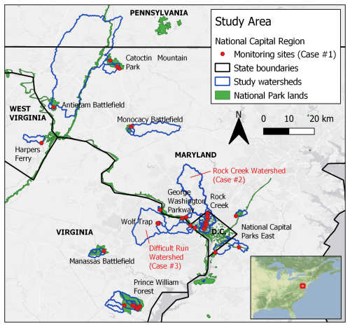
Figure 1 Study area map showing active monitoring sites and all (active + historic) watersheds. Sources: Esri, DeLorme, HERE, MapmyIndia.

Specific conductance (SC) can be used as an indicator of the overall amount of anthropogenic impact to stream water quality in a watershed (Dow and Zampella, 2000). SC data from 2005–2018 for our study sites (Norris et al., 2011) were downloaded from the Water Quality Portal (https://www.waterqualitydata.us/, last access: 9 October 2022). Discrete samples were taken every 1 to 3 months for each site following data quality controls and protocol (Norris et al., 2011), with an average of 179 ± 89 measurements per site. Median SC values over the entire time period were used as the indicator of anthropogenic impacts on each stream for comparison between monitoring sites (Dow and Zampella, 2000). Model calibration data are described in Sect. 2.5.

2.2 Seasonal land cover comparisons

We used Google Earth Engine (Gorelick et al., 2017) to generate a different Dynamic World LULC dataset for the growing season (spring equinox to autumn equinox 2016) and non-growing season (autumn equinox 2015 to spring equinox 2016) for the monitored watersheds by taking dominant LULC data for each pixel over these time periods, following the suggested approach (Brown et al., 2022). Thus, there was one composite image for each season (growing and non-growing) that represented the most common LULC class for each pixel over the time period of individual images, for input into the hydrologic and water quality models. Dynamic World's built class aggregates both hard structures (e.g., buildings and parking lots) and the surrounding vegetation, as is done in other common SWAT LULC inputs such as NLCD developed classes (Brown et al., 2022; Jin et al., 2019). We chose the years 2015–2016 because that period had the earliest available Dynamic World data and was nearest to the center of our 2005–2018 time period for water quality data but repeated the process for every year of available Dynamic World data (2016–2021) for the Rock Creek and Difficult Run watersheds to verify there was a seasonal cycle throughout years (see below). The timing of the data also aligned with the instance of NLCD data from 2016 for comparisons.

2.3 Experimental design

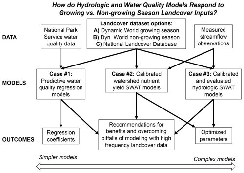
Different watersheds were tested in each case to demonstrate that the seasonal LULC estimate differences were not limited to a single watershed (Fig. 2). For our water quality regressions (case no. 1), we evaluated how well LULC classifications based on Dynamic World data from a single season could identify an LULC forcing, affecting water quality at the watershed scale, following the common regression approach used in water quality investigations worldwide (Fu et al., 2019). We developed quadratic least-squares regression models of median stream SC values over the entire 2005–2018 period for 37 currently monitored NCRN sites explained by seasonal Dynamic World 2016 built LULC. Performance measures R² and the root mean square error (RMSE; Willmott et al., 1985) were used to compare models from different seasons. For the LULC change simulation (case no. 2), we evaluated how a model calibrated to one LULC season could respond to LULC data from another season, such as when simulating impacts of a watershed LULC change, particularly with regards to sensitivity to potential illogical LULC transitions in the high-temporal-frequency data. Here, we developed and calibrated SWAT hydrologic and nitrogen (nitrate N + nitrite N) yield models for the Rock Creek watershed, then used them to simulate a change in LULC classification between growing and non-growing seasons. For the independently calibrated models (case no. 3), we assessed the performance of seasonally tuned models rather than the single model of the LULC change case to provide a fairer comparison of calibrated model performance since each model was optimized to its unique LULC situation. Here, we developed and calibrated SWAT hydrologic models with growing and non-growing season Dynamic World 2016 inputs independently of one another for the Difficult Run watershed. For each case we repeated the analysis with LULC from the commonly used NLCD 2016 for comparison.

Figure 2 Conceptual diagram of the study.

2.4 Soil and Water Assessment Tool

SWAT is the most common water quality model globally (Fu et al., 2019) and has been used in over 6000 peer-reviewed studies (https://www.card.iastate.edu/swat_articles/, last access: 7 January 2024). The SWAT models (rev. 681) used in this study simulated streamflow using a water balance approach (Arnold et al., 1998, 2013), surface runoff using the runoff curve number (NRCS, 1986), groundwater flow using a water balance for shallow aquifer storage (Arnold et al., 1998), snowmelt based on snowpack temperature (Fontaine et al., 2002), and evapotranspiration using the Penman–Monteith method (Monteith, 1965; Ritchie, 1972). Nitrogen yields were simulated based on estimates of runoff, crop use, lateral flow, percolation, and concentrations in soil and water (Arnold et al., 1998). SWAT divides a watershed into spatial subbasins, which may be further divided into unique combinations of soils, land use, and slopes called hydrologic response units (HRUs). HRUs are pertinent to this work as their delineations are in part determined by LULC. HRUs are thus a mechanism by which differences in LULC classification, including erroneous differences derived from seasonality in remote sensing data, can impact the model. Subbasins were delineated using the program QSWAT. In the development of the SWAT models, one spatial data layer for each of elevation, soils, and LULC (Table S1) was input to generate tables that represent base watershed conditions (Abbaspour et al., 2019; Leeper et al., 2015; Lehner et al., 2006; Lindsay, 2014; Sugarbaker et al., 2014; USGS, 2022; USDA, 2022; Ries et al., 2017). We created a new SWAT LULC lookup table for QSWAT to read Dynamic World data and recreate HRUs (Table S2). The Rock Creek models for LULC change simulation (case no. 2) had 13 subbasins, each assigned the dominant HRU, as has been done to more efficiently use computational resources (Myers et al., 2021b; Arabi et al., 2008). Gridded 4 km gridMET historic weather inputs were used as the Rock Creek watershed extends over 30 km from north to south (Abatzoglou, 2013). The Difficult Run SWAT models (case no. 3) had seven subbasins. Our Difficult Run watershed SWAT models were constructed so that the maximum number of HRUs was incorporated (i.e., no minimum HRU area threshold), as has been done to compare independently calibrated model performance (Fuka et al., 2012), with weather data from National Oceanic and Atmospheric Administration (NOAA) station USW00093738 (Table S1). Further descriptions of model HRU numbers and proportions of watershed HRU areas with different LULC inputs can be found in Figs. S4 and S5. We chose the SWAT model for this study because it can be used to support water resource decision-making in mixed-LULC watersheds (Koltsida et al., 2023).

2.5 Sensitivity analysis and calibration

The Rock Creek models (case no. 2) used parameters calibrated with a Latin hypercube approach (to generate a large number of parameter sets; Abbaspour et al., 2004) to the SWAT model with growing season Dynamic World 2016 inputs, using R-SWAT software (Nguyen et al., 2022). R-SWAT is an open-source, graphic-interface, parallelizable, and user-friendly tool to calibrate the SWAT model and analyze results (Nguyen et al., 2022). The parameters optimized during the Latin hypercube approach, which had 2500 iterations (based on Nguyen et al., 2022, and Abbaspour et al., 2004), are shown in Table S3. Calibration and evaluation data were complete monthly streamflow (n= 108 months) and nitrogen (n= 10 months) data from the USGS station 01648010 (concentrations converted to loads by multiplying by streamflow), split with the first half for calibration and the latter half for evaluation at a monthly time step. The years 2013–2021 were used in the simulations as these were the years the USGS station had been active for streamflow, and there was a 3-year model warm-up period (2010–2012) to reduce the influence of initial states. The calibrated parameter set was chosen as having the best performing Nash–Sutcliffe efficiency (NSE; Nash and Sutcliffe, 1970) values for streamflow and nitrogen yield out of the sample of parameter sets.

For case no. 3, sensitivities of Difficult Run watershed SWAT model performance to specific parameters were analyzed using the density-based PAWN method in the Sensitivity Analysis for Everybody (SAFE) toolbox (Pianosi and Wagener, 2015; Pianosi et al., 2015; Zadeh et al., 2017). A total of 8000 SWAT model runs with growing season Dynamic World 2016 data were used for the sensitivity analysis, based on Myers et al. (2021a). We analyzed the sensitivity of 35 parameters and then chose the top 10 parameters with sensitivities greater than the dummy parameter to use in the calibration (Table 1). We then calibrated the Difficult Run watershed SWAT models at a daily time step using the AMALGAM optimization algorithm (Vrugt and Robinson, 2007) with 3200 iterations (based on Myers et al., 2021a) and NSE as the objective function (the metric that the algorithm aims to maximize) and observed daily streamflow from USGS station 01646000 (with the first half for calibration and latter half for validation; Fig. S1). In addition to NSE, metrics for the Kling–Gupta efficiency (KGE; Gupta et al., 2009) and a refined index of agreement (d_r; Willmott et al., 2012) were calculated to confirm our interpretations, with higher values implying better model performance.

Table 1 Parameters used in SWAT model streamflow calibration for the Difficult Run watershed (case no. 3), for model input with growing and non-growing season Dynamic World 2016 data, as well as the model with NLCD 2016 input. Further descriptions of these parameters can be found in Table S4.

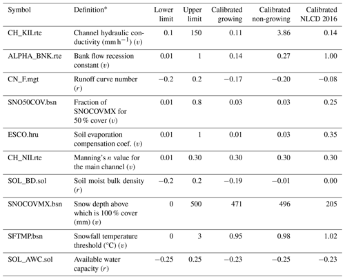
^* A “v” indicates that the original parameter from QSWAT was replaced by the calibrated value globally, in the same unit. An “r” indicates that the original parameter was modified relatively, multiplying it regionally by 1 + the calibrated value (e.g., a value of −0.2 reduces the original parameter by 20 %).

3 Results and discussion

3.1 Seasonal land cover comparisons

The Dynamic World 2016 data classified a greater area of the 55 watersheds as trees during the growing season than during the non-growing season, typically by 5 %–10 % of watershed area (Fig. 3a). During the non-growing season, some areas classified as trees during the growing season were instead given built or shrubland LULC classes. Differences in seasonal LULC classifications in Dynamic World data were strongest in mixed-LULC watersheds (i.e., watersheds with 15 % to 85 % of the area classified as built LULC) and weaker in very low built or very high built percentage watersheds (R²= 0.49, df = 52, F= 24.82, p<0.001; Fig. 3b). There was a relative mean absolute difference (RMAD) of 9.0 % of the watershed area between NLCD 2016 developed (including open space, low, medium, and high intensity) and Dynamic World 2016 growing season built data (5.9 % using non-growing season built data) for the 37 currently monitored watersheds (Fig. S2 and Table S5).

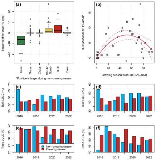
Figure 3 Dynamic World 2016 data. (a) Difference between growing and non-growing season LULC for 55 watersheds (classes of water, flooded vegetation, barren, and snow/ice were approximately 1 % of the watershed area, so they were omitted; boxplots show median, interquartile range (IQR), and outliers outside 1.5 ⋅ IQR). (b) Quadratic relationship between built area and the seasonal difference in built area for 55 watersheds, with 95 % confidence intervals as dashed lines. (c, d) Time series of built-area estimates for the Rock Creek and Difficult Run watersheds, respectively. (e, f) Same as above but for tree area.

The differences between seasons were not limited to a single year of data or watershed and could be more or less pronounced depending on the watershed and time period. For instance, our study watershed for the LULC change simulation (case no. 2, Rock Creek) showed a 9 % increase in built LULC and a 12 % decrease in tree area, in non-growing season relative to growing season Dynamic World data from 2016. Meanwhile, our study watershed for the independently calibrated models (case no. 3, Difficult Run) showed a 12 % decrease in tree cover and a 10 % increase in built areas in the non-growing season compared to the growing season in Dynamic World 2016. Over the entire time period of available Dynamic World estimates for these watersheds, growing season LULC estimates generally had more tree area, while the non-growing season had more built area, and 2016 had the most pronounced differences (Fig. 3c–f). For 2019, when the next instance of NLCD is available for comparisons, differences between non-growing and growing season estimates would be less pronounced for the Rock Creek watershed (+5 % built area and −8 % trees) but approximately the same as 2016 for the Difficult Run watershed (+10 % built area and −11 % trees). In some years such as 2017–2018 the relationship could be reversed. Potential causes for these differences include vegetation phenology (e.g., green up) affected by climate (Khodaee et al., 2022) or measurement artifacts such as atmospheric conditions (aerosol scattering, water vapor, and absorption of light) and reflectance (bidirectional reflectance and zenith angle), which can cause non-random errors in top-of-atmosphere readings used for classifying LULC (Zhang et al., 2018; Kaufman, 1984; Rumora et al., 2020). Dynamic World used a calibrated surface reflectance product to train the classifier (Sentinel-2 Level-2A; L2A) but a top-of-atmosphere product (Sentinel-2 Level 1C; L1C) to generate the dataset (Brown et al., 2022). Previous work in our study area has found strong inter-annual variations across spectral bands in remotely sensed imagery that were caused by uncorrected atmospheric conditions and could impact multi-year LULC classification (Sexton et al., 2013). These differences in atmospheric conditions and reflectance would not be corrected for in Dynamic World data and potentially contribute to differences in classification results over time.

Changes in LULC estimates between seasons were often concentrated along forested edges of mixed-LULC areas (Fig. S3). In these deciduous areas, such as the edges of mixed residential–forested zones, leaf cover decreases during the non-growing season, which could expose other types of LULC underneath or making forest more difficult to distinguish from surrounding built area for the classifications. Actual on-the-ground changes from built LULC to other types or from other LULC types to trees (e.g., succession) are not likely to occur within the short (seasonal) time interval between our LULC composites (Cai et al., 2014).

3.2 Case no. 1: water quality regressions

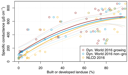
Median stream water specific conductance (SC) was positively correlated with Dynamic World 2016 built LULC during both seasons (Fig. 4; Table 2). This relationship is expected and confirms that urban development has a strong positive effect on surface water salinization (Utz et al., 2022; Kaushal et al., 2005). The model for growing season built LULC vs. median SC had an R² of 0.69, while the same model for non-growing season LULC had an R² of 0.70, and the RMSE's for both models were within three RMSE units (150.16 and 148.08, respectively), which suggests similar performance. For perspective, a model created with developed classes from NLCD 2016 had a fit similar to both seasonal models (R² of 0.66 and RMSE of 155.91; Table 2), supporting the fact that Dynamic World could be relevant for identifying LULC forcings affecting water quality particularly where regional products such as NLCD are not available.

Table 2 Regression models for specific conductance for the growing vs. non-growing seasons of Dynamic World 2016 built data and the model of NLCD 2016 developed classes (df = 34). CI: upper and lower 95 % confidence intervals. Quadratic equation: $a{x}^{\mathrm{2}}+bx+c$.

Figure 4 Modeled median specific conductance (SC) for 37 watersheds comparing Dynamic World 2016 growing and non-growing season built and NLCD 2016 developed LULC, with 95 % confidence intervals as dashed lines.

3.3 Case no. 2: hydrologic and nitrogen yield models

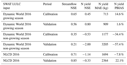
Our Rock Creek watershed SWAT model for streamflow and nitrogen yield, developed and calibrated using Dynamic World 2016 growing season data, performed with a streamflow calibration NSE of 0.56 (validation NSE of 0.65), nitrogen yield calibration NSE of 0.45 (validation NSE of 0.80), and nitrogen yield calibration percent bias (PBIAS; where < 0 implies overestimation bias; Gupta et al., 1999) of 14.6 % (validation PBIAS of 1.6 %) (Table 3). As these values are similar to those of previous SWAT evaluations in urban watersheds that occurred at monthly time steps (Basu et al., 2022; Halefom et al., 2017) and other work with multiple calibration variables (e.g., Myers et al., 2021b), we concluded that the model developed with Dynamic World 2016 growing season data reliably simulated real conditions at a monthly time step (Fig. 5a, b; red circles). When the calibrated parameter adjustments were transferred to the SWAT model developed with non-growing season LULC (as could be done when simulating an actual LULC change), streamflow performance decreased by approximately 0.30 NSE units and nitrogen yield PBIAS became −34.4 % to −57.4 %, implying overestimation of nitrogen (Table 3; Fig. 5a, b; blue circles). Note that both models were run over the same time period to compare performance. Also, the model simulated 50 % greater nitrogen yield over the entire 2013–2021 time period when non-growing season Dynamic World 2016 data were used as the LULC input, rather than growing season LULC (Fig. 5c). These discrepancies between model outputs are not negligible. In relative terms, this difference is greater than the current pollutant load reduction target for Chesapeake Bay of 17 % total nitrogen load (Maryland Department of Environment, 2019). Therefore, we advise taking the potential seasonal variability in LULC estimates into consideration if used to design water quality improvement efforts, particularly when decision-making is involved or an LULC change is being simulated. A model could be fit to one season of LULC but have bias if transferred to a different season of LULC estimates due to temporal inconsistencies. This aligns with previous work that found impacts of actual LULC changes on hydrologic model performance, albeit at longer (e.g., >10-year) time spans (Li et al., 2019). Although hydrologic and water quality models such as SWAT are often developed using LULC classified primarily in the growing season (e.g., Botero-Acosta et al., 2022; Avellaneda et al., 2020), the availability of analysis-ready seasonal LULC data such as Dynamic World makes evaluations of LULC estimate sensitivity at shorter (i.e., seasonal) time spans pertinent.

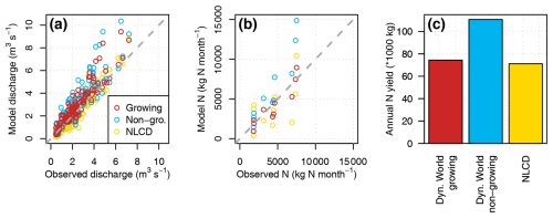
Figure 5 (a) Observed vs. simulated monthly discharge for the Rock Creek watershed comparing Dynamic World 2016 growing and non-growing season built and NLCD 2016 developed LULC. (b) Same for monthly nitrogen (N) yields for Rock Creek. (c) Modeled average annual nitrogen yields for Rock Creek.

Table 3 Model performance metrics for the calibrated Rock Creek hydrologic model (case no. 2) for streamflow and nitrogen yield, based on Nash–Sutcliffe efficiency (NSE), mean absolute error (MAE), and percent bias (PBIAS, where < 0 implies overestimation bias), at a monthly time step. In this case, model parameters were all calibrated to growing season Dynamic World 2016 data to investigate the impacts of simulating an LULC change using non-growing season data (e.g., the optimized parameter adjustments were kept the same).

The differences observed between models using Dynamic World LULC were due to the 9 % increase in built areas in non-growing season Dynamic World 2016 data, which have more impervious surfaces and a higher runoff curve number and generate proportionally more water and nutrient runoff than the forested areas which were classified during the growing season. This could be particularly problematic when using computationally more efficient SWAT models that assign subbasin conditions based on the dominant HRU, as a change in the dominant LULC type in a watershed could result in different subbasin conditions in the model greater than the proportional change in LULC. In this case, using non-growing season instead of growing season LULC input caused the model to switch two HRUs representing 21.9 % of watershed area from being populated with the Dynamic World tree LULC class to the built LULC class (Figs. S4 and S5). For perspective, the nutrient outputs for the SWAT model with Dynamic World 2016 growing season LULC were similar to those simulated by the SWAT model with NLCD 2016 LULC input using the same parameter adjustments (Fig. 5c).

3.4 Case no. 3: independently calibrated hydrologic models

The individually calibrated SWAT models using growing season vs. non-growing season Dynamic World 2016 LULC input for the Difficult Run watershed had comparable performance when simulating streamflow, despite the differences in LULC inputs (10 % increase in built areas and 12 % decrease in tree cover for the non-growing season LULC input). NSE performance metrics at a daily time step were between 0.52 and 0.54 for each model with Dynamic World LULC over the calibration and validation time periods, KGE was between 0.61 and 0.75, and d_r (which by not squaring errors provides a better measure of low-flow performance) only ranged between 0.68 and 0.70 (Table 4; scatterplots in log scale to show daily baseflows and time series are presented in Fig. 6a–d). These are in line with satisfactory performance from previous work, particularly considering a daily time step (Moriasi et al., 2007; Kalin et al., 2010; Basu et al., 2022). For perspective, the SWAT model calibrated with NLCD 2016 LULC had an NSE of 0.48 for the calibration period and 0.47 over the validation period (Table 4). Discrepancies such as underestimated low flows or peaks could reflect difficulties in simulating hydrology in urban areas with complex stormwater pathways, as the Difficult Run watershed was 58 % developed area in the NLCD 2016 data. Also, differences between independently calibrated streamflows could be smaller than differences with observed data, which could be due to uncertainties in other non-LULC model inputs shared among the calibrations (Basu et al., 2022). At the HRU level, using growing vs. non-growing season Dynamic World 2016 LULC in this case resulted in a 12.8 % change in model HRU tree proportions, which is proportionate to the change in input tree estimates, as would be expected with the maximum HRU designation approach (Figs. S4 and S5).

Table 4 Comparison of streamflow performance for calibrated SWAT models developed independently with Dynamic World 2016 growing season LULC input, Dynamic World 2016 non-growing season LULC input, and NLCD 2016, at a daily time step for the Difficult Run watershed (case no. 3). Performance indices are R², the Nash–Sutcliffe efficiency (NSE), the Kling–Gupta efficiency (KGE), and a refined index of agreement (d_r).

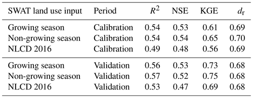
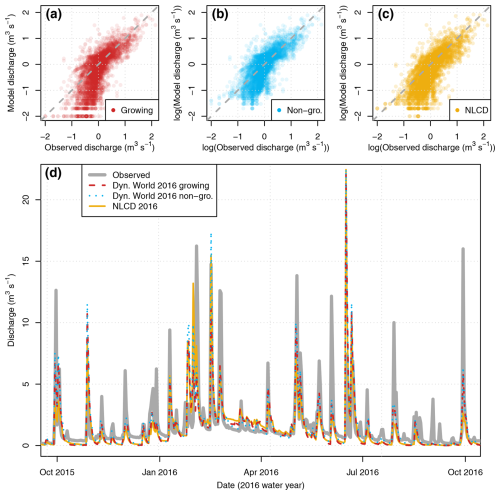
Figure 6 Daily discharge models for the Difficult Run watershed displaying a base-10 log so that daily baseflows and low flows are visible, comparing independently calibrated models with (a) Dynamic World 2016 growing season LULC, (b) Dynamic World 2016 non-growing season LULC, and (c) NLCD 2016. (d) Time series of Difficult Run modeled discharge.

The most sensitive parameters for the Difficult Run watershed case were the channel hydraulic conductivity (CH_KII), bank flow recession coefficient (ALPHA_BNK), and runoff curve number (CN_F) (Fig. 7). Among these and other sensitive parameters, there were differences in optimized values depending upon the SWAT LULC input (Table 1). For example, the CN_F adjustment was optimized to −0.17 for growing season Dynamic World 2016, −0.20 for non-growing season Dynamic World 2016, and −0.08 for NLCD 2016 inputs, suggesting that the optimization adjusted runoff processes to compensate for the different proportions of LULC. The difference in forests of 12 % of watershed area between growing and non-growing season Dynamic World 2016 data for Difficult Run (Table S5) is as large a difference as real changes in forests that have been found to cause these sensitivities in model parameters (Li et al., 2019) but was likely caused by classification variation rather than an actual cycle from trees to built area and back (Hermosilla et al., 2018). It is critical to consider that the differences in parameter values create the potential for the models to respond differently to future changes in LULC or climate change due to variations in unmeasured water balance outputs (Myers et al., 2021a). Also, although we did not investigate equifinality using model ensembles for this case, we aimed to limit it by employing a calibration approach with multiple optimization algorithms (AMALGAM; Vrugt and Robinson, 2007) and calibrating only the most sensitive parameters. Previous work has found this approach to be robust to equifinality relative to other factors affecting parameter optimizations such as calibration/validation time period selection (Myers et al., 2021a) and model structures (Myers et al., 2021b), and our findings are in line with previous investigations of LULC input changes impacting SWAT model parameter optimizations (such as forest conversion causing runoff curve number adjustment to relatively vary by 21 %; Li et al., 2019).

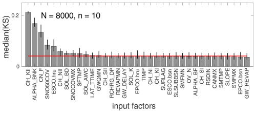
Figure 7 PAWN sensitivity analysis results ranking the SWAT parameters from most to least sensitive, using 8000 samples (N) and conditioning intervals (n) of 10. The red line is the “dummy” parameter, and bars are 95 % confidence intervals. KS: Kolmogorov–Smirnov statistic. Higher median KS indicates higher sensitivity of SWAT model streamflow output to the parameter. Readers are directed to Table S4 and Arnold et al. (2013) for further documentation of these input factors.

3.5 Future directions

Illogical LULC classifications related to seasonal differences in remote sensing data could be pertinent to models beyond our cases of regressions and SWAT in the eastern United States, such as models for which accurate parameterization of LULC processes is essential for simulating the impacts of climate change (Glotfelty et al., 2021). For instance, potential seasonal variation in LULC estimates should be considered during an LULC update in a modeling approach such as Hales et al. (2023), where the global hydrologic model GEOGloWS is bias-corrected for extreme event forecasting in underdeveloped regions using a single instance of Dynamic World data. Our findings show that there is the potential for discrepancies at least for temperate watersheds in the eastern United States if the season for the LULC update were not accounted for. These illogical LULC changes could also be pertinent for models that can use a mosaic approach to represent spatial variability in LULC within coarser grid cells (e.g., CLM5; Lawrence et al., 2019). The mosaic approach assumes that land surface properties (e.g., water fluxes) are homogeneously related to the LULC type (Li et al., 2013; Qin et al., 2023), in which case an illogical conversion of 12 % area from forest to other types (our case no. 3 example) could carry forward into the models and potentially impact water and energy flux estimates or parameterizations similar to an actual LULC change. For instance, deforestation has previously been shown to alter heat and carbon fluxes and ecosystem productivity in CLM5 (Marufah et al., 2021; Luo et al., 2023). Variability within input data subgrids has also been shown to influence model parameter optimization and performance simulating hydrology, making it an important aspect to account for (Samaniego et al., 2010). As models advance into higher spatiotemporal resolution following increasing computational resources and data availability (e.g., Hales et al., 2023), we encourage the modeling community to be cognizant of the potential impacts of illogical seasonal LULC change, such as we identified for mixed-LULC areas of the eastern United States. The strength of the effect of the illogical seasonal LULC change on the model outputs and optimized parameters would depend on many factors including model processes and spatiotemporal extent. A model intercomparison study in this regard would likely be a meaningful contribution to the advancement of the field regarding higher spatiotemporal capabilities.

When using seasonal LULC estimates in hydrologic and water quality models, we recommend differentiating HRUs as much as possible (like our approach of maximum HRU resolution for case no. 3) so that the potential for disproportionate impacts from the LULC season is minimized. Aggregating HRUs by dominant characteristics over an area may lead to high variability in responses depending on areas where estimated LULC changes are substantial enough to switch dominant HRU LULC characteristics, which in our second case was two HRUs in the northern part of the watershed. However, future work could investigate approaches to differentiate HRUs that further limit or remove the impacts of seasonal variation in LULC estimates, such as separating areas with stable LULC across seasons from those with substantial LULC variability to isolate the most affected parts of the watershed. Thus, HRUs that remain unaffected by seasonal changes in LULC estimates would be preserved, while HRUs with potential for change due to illogical seasonal LULC transitions could be identified and treated separately. In this proposed approach, aggregating HRUs may be possible to resist disproportionate impacts of LULC seasonality while alleviating computational burdens of large HRU numbers. Evaluation of such an approach could help advance the hydrologic and water quality modeling community regarding higher-spatiotemporal-resolution LULC capabilities.

The impacts of seasonal land cover inconsistencies on geospatial models could yield several additional future research directions that build upon our findings. As our study used watershed-scale water quality and quantity investigations, further work should investigate how seasonal LULC classification inconsistencies could affect assessments of habitat, biodiversity, land management, ecology, global hydrology, and future climate based on LULC change (Yang et al., 2022; Di Vittorio et al., 2018; Hales et al., 2023; Hood et al., 2021). It may be particularly useful to explore whether the high-resolution, high-frequency LULC data could be used in the LULC change models (e.g., Hood et al., 2021) to improve the temporal precision of interpolations between discrete LULC images. Future work could also investigate how seasonal LULC classification inconsistencies influence models outside our temperate study area (e.g., mountainous, arid, tropical, high-latitude, savannah, Mediterranean, continental) to gain a broader understanding of global geospatial model impacts. The use of high-frequency monitoring data (Zhang et al., 2023) could be explored to investigate the influence of high-temporal-resolution LULC on water quality patterns, as well as whether a modification to environmental models such as time-varying parameters (Li et al., 2019) could account for the seasonal differences in Dynamic World LULC classifications. Future research could also incorporate LULC pixel probabilities from the Dynamic World dataset (Brown et al., 2022; Small and Sousa, 2023) into geospatial models and investigate their utility for environmental fields. Post-processing approaches for high-temporal-resolution LULC products to address seasonal inconsistencies (Sexton et al., 2013; Liu and Cai, 2012; Hermosilla et al., 2018; Zhao et al., 2019) could aid in alleviating the impacts of seasonal inconsistencies that cause model sensitivities as well. Finally, future work could investigate which seasons of LULC data are most accurate for different purposes, such as vegetation or impervious surface classification, and how causes of year-to-year inconsistencies in seasonal LULC estimates could affect models.

4 Conclusions

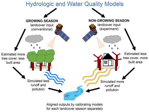
When seasonal changes in LULC data occur, due to classification difficulties such as vegetation cycles (e.g., deciduous leaf cover in mixed-LULC areas), hydrologic and water quality models developed using growing season LULC inputs could behave differently from those using non-growing season LULC (Fig. 8), with meaningful differences for environmental efforts such as pollutant load reduction targets. The cause in temperate watersheds is primarily a sensitivity to changes from built to forest LULC proportions that affects modeled runoff and nutrient yields, representing temporal classification inconsistencies rather than actual succession or restoration. Environmental and geospatial researchers should be aware of this sensitivity when developing models and assessing changes in LULC as they relate to water quantity and quality, especially when considering the use of different seasons of available LULC data in a model. The seasonal variation in Dynamic World LULC data we identified is pertinent for environmental models of future climates, biodiversity, habitat loss, land management, ecology, and biogeochemistry that are dependent on precise assessments of LULC change that could be affected by the seasonal classification variation. With a limited geographic scope (e.g., temperate watersheds) and small sample of models, our work does not intend to show definitively when, where, or in what model configurations these sensitivities would occur but that they are a possibility that modelers should be aware of. We discussed future research directions which could advance capabilities regarding the use of high-spatiotemporal-resolution global LULC information such as Dynamic World for geospatial models across disciplines.

Figure 8 Conceptual diagram of the conclusions of the study in temperate watersheds of the eastern United States.