On the challenges of global entity-aware deep learning models for groundwater level prediction

The application of machine learning (ML) including deep learning models in hydrogeology to model and predict groundwater level in monitoring wells has gained some traction in recent years. Currently, the dominant model class is the so-called single-well model, where one model is trained for each well separately. However, recent developments in neighbouring disciplines including hydrology (rainfall–runoff modelling) have shown that global models, being able to incorporate data of several wells, may have advantages. These models are often called “entity-aware models“, as they usually rely on static data to differentiate the entities, i.e. groundwater wells in hydrogeology or catchments in surface hydrology. We test two kinds of static information to characterize the groundwater wells in a global, entity-aware deep learning model set-up: first, environmental features that are continuously available and thus theoretically enable spatial generalization (regionalization), and second, time-series features that are derived from the past time series at the respective well. Moreover, we test random integer features as entity information for comparison. We use a published dataset of 108 groundwater wells in Germany, and evaluate the performance of the models in terms of Nash–Sutcliffe efficiency (NSE) in an in-sample and an out-of-sample setting, representing temporal and spatial generalization. Our results show that entity-aware models work well with a mean performance of NSE >0.8 in an in-sample setting, thus being comparable to, or even outperforming, single-well models. However, they do not generalize well spatially in an out-of-sample setting (mean NSE <0.7, i.e. lower than a global model without entity information). Strikingly, all model variants, regardless of the type of static features used, basically perform equally well both in- and out-of-sample. The conclusion is that the model in fact does not show entity awareness, but uses static features merely as unique identifiers, raising the research question of how to properly establish entity awareness in deep learning models. Potential future avenues lie in bigger datasets, as the relatively small number of wells in the dataset might not be enough to take full advantage of global models. Also, more research is needed to find meaningful static features for ML in hydrogeology.

1 Introduction

Groundwater is the primary drinking water resource in Germany (Hoelting and Coldewey, 2013) and a major resource worldwide (WWAP, 2015). As such, it is under growing pressure due to, e.g. climate change, increased drought frequencies, or irrigation (WWAP, 2015). All of these transient drivers of change highlight the utmost importance of functional groundwater management, for which groundwater level prediction models are a key tool (Wada et al., 2010; Famiglietti, 2014; Bierkens and Wada, 2019). For functional national groundwater management, groundwater models need to be available on large or national scales. While some conceptual modelling approaches do exist that meet this criterion (Ahamed et al., 2022), they generally lack sufficient local-scale accuracy (Gleeson et al., 2021). Currently, distributed numerical models are the dominant hydrogeologic model class in groundwater level modelling. However, while being an excellent tool to answer tangible questions in complex local to regional hydrogeologic settings, numerical models do not scale well. It is not trivial to parameterize larger-scale numerical models because it is an expensive process. The process needs some degree of subjective sophistication and depends on numbers of unstructured geological or spatial data.

The ability of machine learning algorithms, especially neural networks, to incorporate large numbers of data and to let them sort out the complexity themselves in order to make highly accurate predictions on the point scale makes them a useful tool for closing this gap. With large-scale applicability also comes the potential to realize prediction in ungauged aquifers (PUA), as put forward by Heudorfer et al. (2019) and Haaf et al. (2020, 2023), in a global, generalizable way. The idea of PUA is inspired by the widely known concept of prediction in ungauged basins (PUB) in rainfall–runoff hydrology (Sivapalan et al., 2003; Hrachowitz et al., 2013). As the name says, PUA refers to the aim of setting up models that are capable of predicting groundwater levels in areas where no groundwater data are sampled, i.e. ungauged areas. This can be large areas with no or sparse monitoring, but also areas in between groundwater monitoring wells in well-monitored regions. As groundwater dynamics can change within rather short distances due to heterogenous aquifer or infiltration conditions, such models could be used to create spatially continuous data out of point measurements at monitoring sites. Continuous groundwater level data are of great importance, because they serve as a basis for important decision-making tasks, such as deriving protection zones.

Even though the application of machine learning approaches in hydrogeology gained some traction in recent years, the field is still emerging. In a recent review, Tao et al. (2022) recapitulated that neural network architectures often prove to be superior to other machine learning model classes. Thereby, state-of-the-art groundwater level prediction with neural networks is mostly based on single-well models, where a single neural network model is trained for each groundwater well (Tao et al., 2022; Wunsch et al., 2021b, 2022a; Rajaee et al., 2019). While excellent fits can be achieved this way at the level of individual wells, the big drawback is that it is not possible to generalize or even regionalize with these models. A model that is capable of overcoming this drawback is called a “global model”, where “global” means encompassing the whole dataset available. This model class made a first appearance in hydrogeology's sister field, hydrology, through the works of Kratzert et al. (2018, 2019a, b) in the task of rainfall–runoff modelling. They showed (Kratzert et al., 2019b) that a neural network can use static features (such as time-series features or environmental features, see below) to distinguish individual dynamic input features (meteorological) and target features (there: runoff) relations in a meaningful way, thereby allowing the model to generalize to locations with similar combinations of static features. They called this set-up an “entity-aware model” (Kratzert et al., 2019b), a term which is also common among various disciplines that use entity characteristics to model personalized prediction of responses for individual entities caused by external drivers (Ghosh et al., 2023).

While there have been approaches of global models for groundwater level modelling (e.g. Clark et al., 2022) or groundwater abstraction modelling (e.g. Majumdar et al., 2020, 2022), to the best of the authors' knowledge, the concept of entity-aware global modelling has not been transferred to hydrogeology to date. The reason might be that providing the model with a set of static features that is able to capture the hydrogeologic dynamics of the system in a conceptual way is much more difficult than in other disciplines, due to the complex nature of underground flow. Even though hydrology and hydrogeology are strongly related disciplines (Barthel, 2014), the question is whether the global entity-aware approach will work similarly well in hydrogeological conditions, which exhibit substantially more heterogeneous and “local” groundwater dynamics (Heudorfer et al., 2019), which is why nearby wells do not necessarily have high time-series similarity (Wunsch et al., 2022b). It is not trivial to expressively link environmental static features taken from geospatial or geologic data products to groundwater dynamics (Haaf et al., 2020), also because of uncertainties in these products, which are often only regionalized data from point measurements, such as for hydraulic conductivity or depth to groundwater.

For this reason, we test two different versions of a hydrogeologic global entity-aware model: the time-series feature-driven model (TSfeat model) and the environmental feature-driven model (ENVfeat model). Both models have different potential applications. The ENVfeat model uses static environmental features that are available spatially and continuously (see Sect. 2.2 for more information). It represents the gold standard of a fully generalizable and regionalizable model that we seek to achieve, in order to reach the overarching goal of PUA. However, geospatial data of sufficient quality to be used in machine learning are not always available. Also, the aforementioned lack of representativity of geospatial proxy data with regard to groundwater dynamics (Haaf et al., 2020) hypothetically hampers predictability in a hydrogeologic ENVfeat model. Thus, the TSfeat model is the viable alternative that retains the property of generalizability. The TSfeat model differentiates groundwater time series in multi-well prediction based on static time-series features that are derived from the past groundwater time series itself (Heudorfer et al., 2019; Wunsch et al., 2022b, see Sect. 2.2). A TSfeat model can therefore hypothetically work on any existing monitoring network, being able to incorporate additional unseen groundwater data and thus generalize on groundwater data alone, despite lacking the ability to regionalize in the sense that it cannot predict groundwater head based on secondary data sources (i.e. geospatial data) like the ENVfeat model can. We argue that time-series features are best suited to describe the dynamics of an individual time series, and to best distinguish different groundwater dynamics from each other, thus hypothesizing that the TSfeat model outperforms the ENVfeat model.

In general, both “global” model types have the theoretical advantage of more data compared to single-well models, i.e. data of similar wells regarding dynamics can contribute to the training of, e.g. wells with few training data and thus enhance their performance. To further test our hypotheses, we compare additional model set-ups, one where the set of environmental or time-series static features are replaced by a set of completely random static features (RNDfeat models), and one with no static features at all, relying only on the dynamic inputs (DYNonly model).

Regarding architecture, long short-term memory neural networks (LSTMs) and convolutional neural networks (CNNs) are currently equally dominant model classes in machine learning (ML)-guided groundwater level modelling, as they consistently deliver high-class performance while maintaining some degree of model simplicity (Tao et al., 2022). LSTMs are an especially common architecture for sequence modelling in hydrological settings (Kratzert et al., 2018, 2019a, b), but also increasingly in groundwater (Tao et al., 2022; Rajaee et al., 2019). LSTMs are an improved version of simple recurrent neural networks (RNNs) and overcome the RNN drawback of limited memory of only few time steps (Bengio et al., 1994), which makes LSTMs suitable for time-series modelling. They do so by introducing a cell memory state as well as an input gate, forget gate, and output gate to control information storage and dissipation when flowing through the LSTM layer during training (Hochreiter and Schmidhuber, 1997). For a while, transformer architectures seemed promising candidates to generally supersede LSTMs in sequence modelling, but their suitability as a general-purpose method beyond their original domain (language modelling) is increasingly called into question because they can be outperformed by simpler linear neural models (Zeng et al., 2023), notably across the board (Das et al., 2023). In the neighbouring discipline of groundwater quality modelling, extreme gradient boosting (XGB) proved to be a powerful alternative (Bedi et al., 2020; Ransom et al., 2022; Haggerty et al., 2023). However, groundwater-quality modelling is a related but different field from groundwater-level modelling with a number of significant differences, making the methods not directly transferable. Thus, currently, LSTM and CNN methods remain the state of the art in groundwater level modelling. In the present study, we use an LSTM in the global model set-up to learn the input–output relationship of meteorological forcing data and groundwater level, and combine it with a multi-layer perceptron (MLP) for processing the static features. This is despite precursor studies by Wunsch et al. (2021b, 2022a) resorting to the CNN architecture for the single-well set-up, as in their study, better performance and stability were achieved with CNNs. However, in the (global) use case presented here, LSTM showed overall better performance in preliminary experiments (see Fig. A1 in the Appendix), and thus an LSTM architecture was chosen.

The aim of this study is to test whether the concept of entity-aware global deep learning modelling is transferable to groundwater level prediction, and, if so, which set of static features are best suited to do so. First, we introduce the dynamic (Sect. 2.1) and static (Sect. 2.2) feature data used in the study. We then give an overview of the model architecture and optimization strategy (Sect. 3.1) and an outline of the experimental design (Sect. 3.3), followed by a brief introduction of the state-of-the-art learning rate scheduling method to help learning (Sect. 3.2). We then compare the model performance of the ENVfeat, TSfeat, RNDfeat, and DYNonly model variants (Sect. 4.1) and discuss possible reasons for the differences in performance. We further analyse feature importance (Sect. 4.2) to get to the bottom of performance differences. The paper ends with concluding remarks and an outlook in Sect. 5.

2 Data

2.1 Dynamic feature data and study area

Regarding groundwater level data, the dataset of Wunsch et al. (2022a) is used in this study. This dataset consists of 118 weekly groundwater level time series from the uppermost unconfined aquifer layer, whose groundwater dynamics are mainly dominated by climate forcing. The wells are relatively evenly distributed across Germany, as can be seen in Fig. A2. The dataset was primarily chosen because it is pre-published and readily available from an open-source repository, enabling reproducibility and ease of publication. For additional information on the dataset and details on data pre-processing routines, please refer to Wunsch et al. (2022a). Based on this readily available dataset, the only additional pre-processing step was to exclude time series with start dates after 1 January 2000 and end dates before 31 December 2015. This was done to make sure that enough data are present for good model results. Also, four individual time series were excluded manually because of missing environmental static feature data (see Sect. 2.2). This resulted in a total number of 108 groundwater time series used in this study.

Dynamic input features used in this study are precipitation (P), temperature (T), and relative humidity (RH) from HYRAS 3.0 (Rauthe et al., 2013; Frick et al., 2014), which proved its suitability in several previous studies (Wunsch et al., 2021b, 2022a), as well as an annual sinusoidal curve fitted to temperature (T_sin), which was also shown to be a valuable driving variable (Wunsch et al., 2021b). HYRAS 3.0 is a 1×1 km gridded meteorological dataset covering German national territory, with data ranging from 1951 to 2015. The dataset is essentially the same as in Wunsch et al. (2022a); however, the HYRAS RH and the fitted sinusoidal curve were used here additionally.

2.2 Static feature data

It is well known that no single static feature is able to describe the totality of control on groundwater dynamics, but a combination of features can provide a good approximation (Heudorfer et al., 2019). Consequently, exhaustive yet compact sets of static input features were compiled. Thereby, two separate sets of static features were fed into two separate model set-ups: time-series features and environmental features. The first type (time-series features) are quantitative metrics calculated from the groundwater time series themselves and express certain aspects of dynamics in these time series. There is a long history of studies in hydrology and to a somewhat lesser extent in hydrogeology (see Introduction by Heudorfer et al., 2019, for a brief review) dedicated to finding, improving, and analysing which time-series features best depict certain aspects of time-series dynamics, or the totality of time-series dynamics in a reduced set of time-series features. Oftentimes redundancy analyses, correlation analyses, dimensionality reduction, or similar methods are conducted to determine a suitable set of features. As a conceptual decision, we use the set of time-series features devised by Wunsch et al. (2022b). This set constitutes a small and manageable, redundancy-reduced set of time-series features that was furthermore successfully applied in past studies to cluster time series in the larger dataset of wells (Wunsch and Liesch, 2020; Wunsch et al., 2022b) from which the sample of wells used in this study is taken (see Sect. 2.1). The full list of time-series features used in this study, along with descriptions, can be found in Table 1.

Wunsch et al. (2022b)Wunsch et al. (2022b)Wunsch et al. (2022b)Wunsch et al. (2022b)Wunsch et al. (2022b)Wunsch et al. (2022b)Wunsch et al. (2022b)Heudorfer et al. (2019)Richter et al. (1996)

Table 1 Static time-series features used in the TSfeat model variant. Features were derived from the groundwater level (see Sect. 2.1) from the beginning of the time series until 2011 (to exclude the test period from 2012 onwards). Table taken from Wunsch et al. (2022b).

BGR (2019)BGR (2003)BGR and SGD (2015)BGR and SGD (2019)BGR and SGD (2019)BGR (2018)Hengl et al. (2017)Hengl et al. (2017)Beven and Kirkby (1979)Noelscher et al. (2022)Noelscher et al. (2022)Noelscher et al. (2022)European Union et al. (2018)DWD Climate Data Center (CDC) (2023)

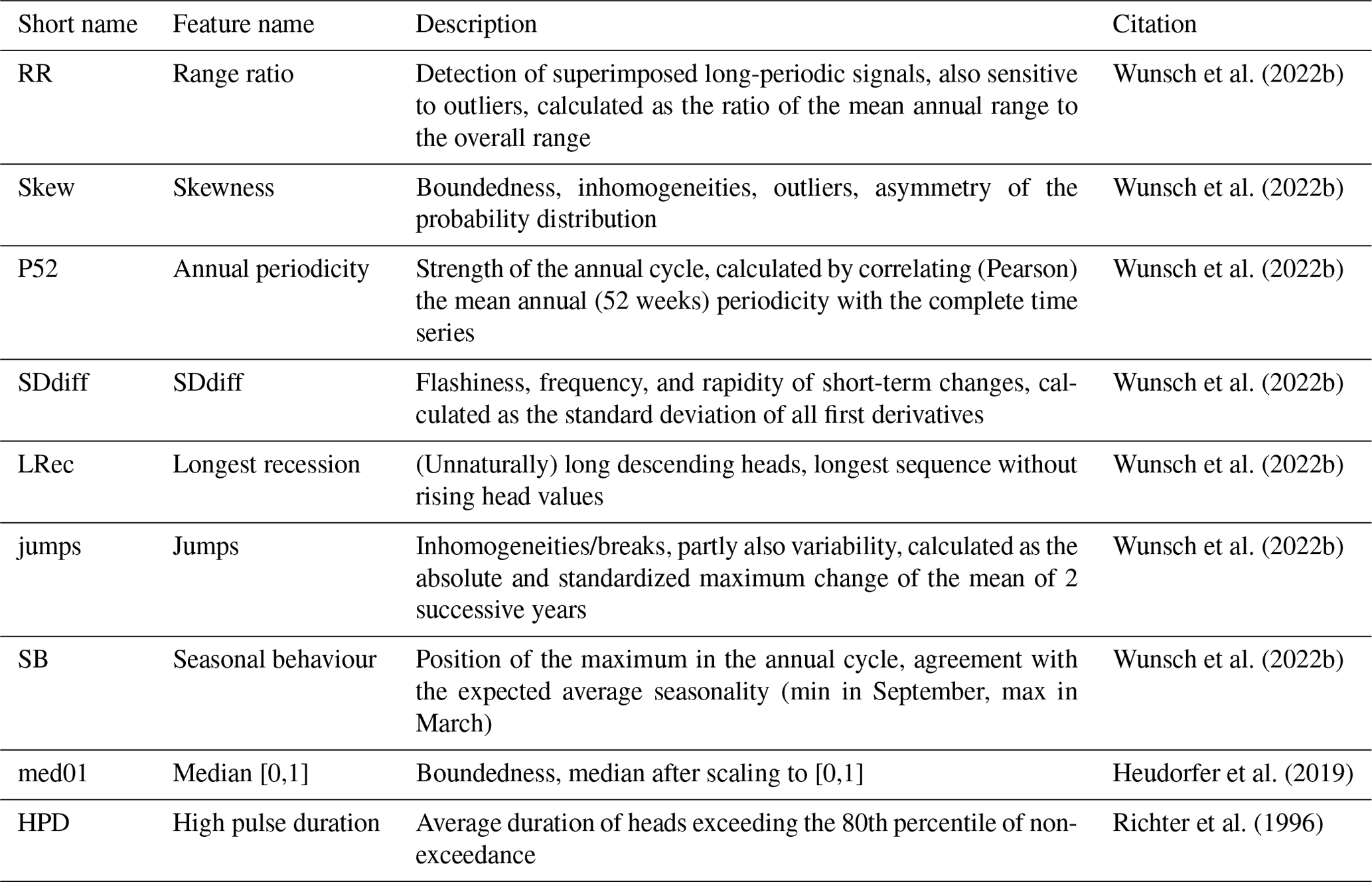
Table 2 Environmental static features used in the ENVfeat model variant. Hydrogeologic, soil, topographic, and land cover features as well as ETpot were derived from map products by sampling the map value at the location of the groundwater well. Climatic static features with exception of ETpot were derived from the meteorologic dynamic input features (see Sect. 2.1) in the period from 1991 (to match ETpot data availability) to 2011 (to exclude the test period from 2012 onwards).

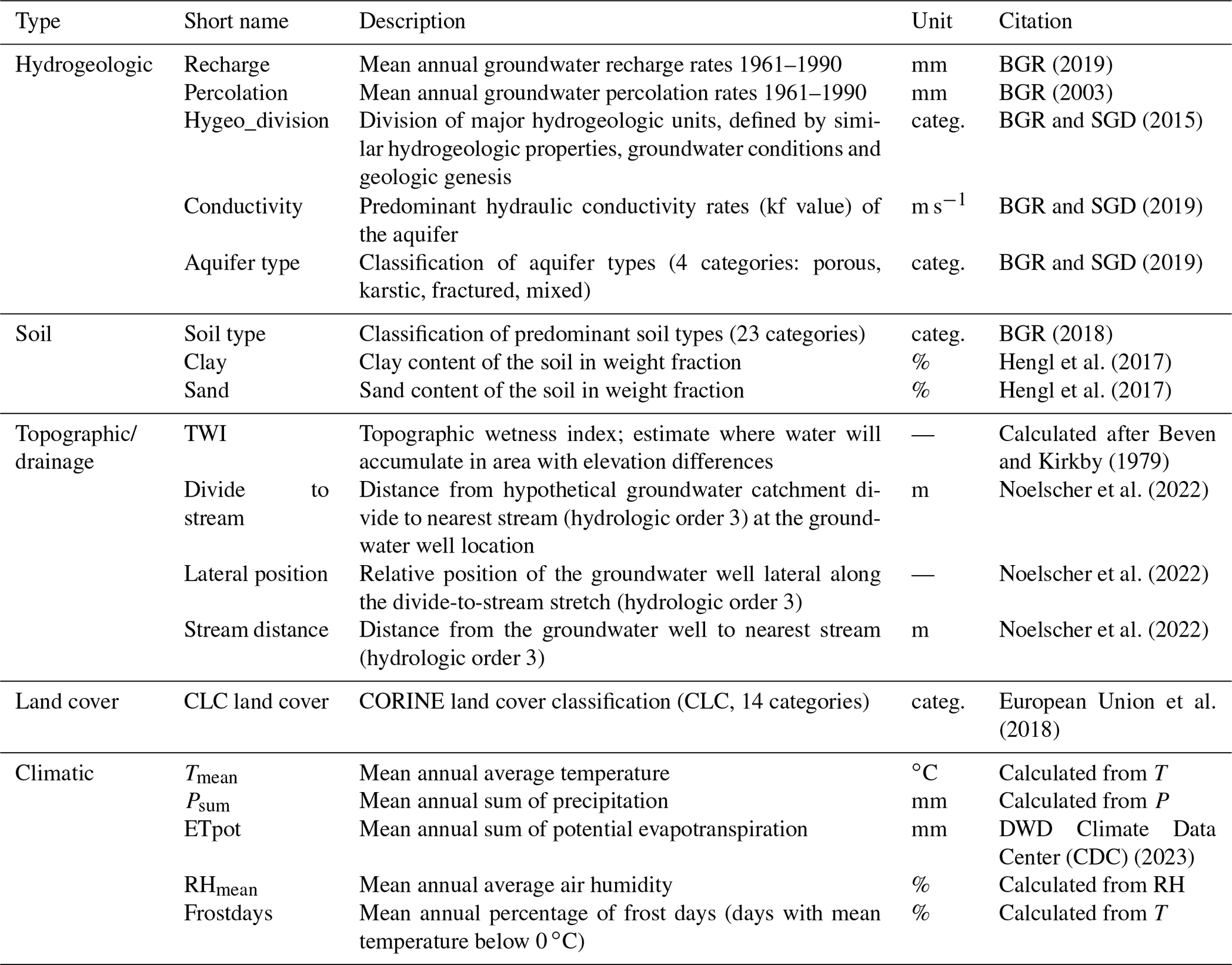
The second type of features, environmental features, are descriptors of the hydrogeological, physiographic, and climatic functioning of the underground and landscape. They are proxies for environmental factors controlling groundwater recharge and flow and thus the dynamics in groundwater time series (Haaf et al., 2020). To be able to reach the stated goal of PUA (see Sect. 1), it is important that environmental features used in the model are spatially continuously available across the study domain (Germany). Thus, only nationwide geospatial datasets are considered in the selection that are, for the sake of reproducibility, freely available. Moreover, we use datasets that are not too fine-grained (in the case of categorical data), in order to ensure that each category is represented by one or more monitoring wells. This means that when multiple-source datasets for the same type of environmental feature are available, the one with the better (usually higher) degree of aggregation was chosen. For example, for soil type, there is a product called “buek200” with more than 550 categories (BGR, 2018), and another product called “buek5000” (BGR, 2005) which is a generalized version of buek200 and has only 23 categories. In that case, Buek5000 was chosen because communality of soil type categories between groundwater locations would be impossible with buek200, given the limited size of our groundwater dataset.

In surface hydrology, the science of identifying major controlling factors for river flow systems is mature enough to yield large-scale or even global selection datasets of environmental features with which river flow can be predicted and explained in an exhaustive way (e.g. Addor et al., 2017; Linke et al., 2019; Kratzert et al., 2019b, 2023). In hydrogeology, this is not the case yet. No comparable selection of tried and tested sets of environmental features controlling groundwater dynamics is available that could be used in ML-based prediction of groundwater head. In light of this, we compiled a first selection that is summarized in Table 2. It was assembled primarily by conceptual decision from available geospatial datasets to cover the five major domains of control, namely hydrogeology, soil, topographic drainage, land cover, and climate. Specifically, climate can be of transient nature, which is why it was used as a long-term average over the whole study period. Also, land cover can technically be transient, e.g. in highly dynamic developing countries. However, land cover in Germany can be assumed to be static during the study period with a high degree of confidence. Some factors such as, e.g. depth to groundwater, which are important factors based on conceptional understanding, are omitted, due to the aforementioned reasons of data availability. Thus, this selection should be seen as a starting point to serve the proof of concept in this study.

To ground-truth the effect of the static environmental and time-series features, a third set of static features was used, by replacing the number of static features with random counterparts of equal size, i.e. sets of randomly generated integers in the range of 0–9. This was done in two variants, one set with nine random integers to equal the number of time-series features (RNDfeat9), and one set with 18 random integers to equal the number of environmental features (RNDfeat18). These numbers were chosen to make sure that all aspects but the values of the static features themselves match the model set-up of the TSfeat and the ENVfeat models so as to exclude other influences.

All numeric static features (time series, environmental, or random) were standard scaled before feeding them into the model. All categorical static features (only environmental) were one-hot encoded.

3 Methods

3.1 Model architecture and optimization strategy

We use LSTMs in a global entity-aware model set-up to learn the input–output relationship between dynamic (meteorological) input features and groundwater level as the target feature. LSTM was chosen over CNN because it proved to be superior to CNN in the global entity-aware model set-up in preliminary studies (see Fig. A1 for a comparison). To allow the global model to distinguish between different groundwater dynamics of individual wells, static input features that differentiate the wells must be fused to the dynamic (meteorological) input features. Different approaches exist to accomplish this data fusion. Most notably, Kratzert et al. (2019a, b) provide two separate variants to accomplish data fusion. The first is the basic variant where static features are simply concatenated to the meteorological inputs at each time step, together entering the model through the same input layer. The second is more sophisticated with a modified LSTM layer where static features control the input gate, and the dynamic features control the forget gate, output gate, and memory. Even though the modified LSTM layer variant provides desirable levels of interpretability, the basic data fusion variant notably outperformed it (Kratzert et al., 2019b). Thus, we disregard the modified LSTM layer variant in this study. But as discussed in Miebs et al. (2020), also the basic data fusion variant is not an optimal choice for RNN architectures, since such an approach leads to a significant increase in the number of RNN parameters due to the fact that duplicated static features are evaluated each time for every sequence, while not adding any meaningful additional information. As a consequence, training becomes more memory- and time-consuming at comparable outcome (Miebs et al., 2020). Thus, instead of the simplistic basic duplication variant, we use a model architecture where data fusion of dynamic and static input features is achieved by providing separate model threads that process the dynamic and static inputs individually and are later concatenated (Fig. 1), as also used and put forward by, e.g. Miebs et al. (2020), Liu et al. (2022).

In this model, for every time step being processed, a sequence of the previous 52 time steps (making up 1 full year) of the four dynamic input features P, T, T_sin, and RH is given to an LSTM layer of size 128 in the dynamic model thread. In the same time step, one set of static feature values, associated with the well whose groundwater head is currently being processed, is fed into a multi-layer perceptron (MLP) of one fully connected (Dense) layer of size 128 in the static model thread. Subsequently, outputs of both threads are concatenated and fed into another MLP with a Dense layer of size 256, which again feeds into an output Dense layer of size 1. In the whole architecture, all neural layers (despite the output) are followed by a dropout layer with a dropout rate of 0.1 for regularization.

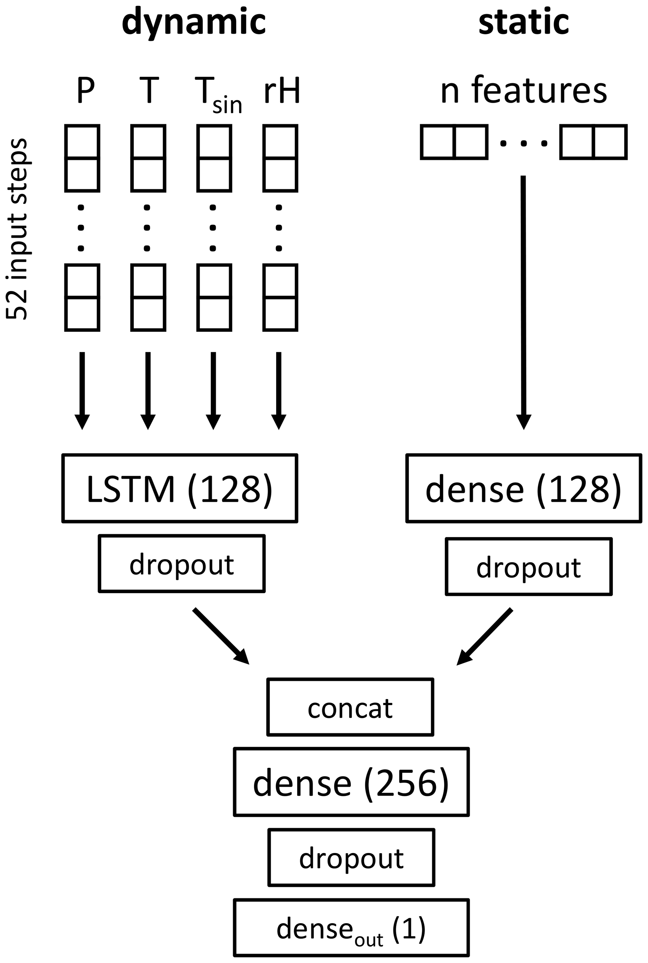
Figure 1 The double-threaded global entity-aware model architecture introduced in this paper. Hyperparameters not found in the figure are reported in the text or can be found in the associated code.

For every well separately, both groundwater and meteorological time series were split into three parts: training set, validation set, and test set. To ensure comparability of performance between wells in light of interannual (or even interdecadal) fluctuations in groundwater, we chose to set a fixed period for the validation and test sets. The validation period was scheduled 1 January 2008–31 December 2011, and the test period was scheduled 1 January 2012–31 December 2015, which is 4 years each. The training period was left open towards the past, meaning the model takes various time-series lengths during training, under the sole condition that training data are available at least from 2000 onwards, i.e. at least 8 years of training data (see Sect. 2.1).

The model was optimized with the Adam optimizer (Kingma and Ba, 2014) on the mean square error (MSE) loss function during training, and later evaluated based on Nash–Sutcliffe efficiency (NSE) calculated from model errors in the test set, while the coefficient of determination (R²) as well as the root mean square error (RMSE) are reported in this paper merely for comparison. This way of calculating the NSE metric is directly adapted from (Wunsch et al., 2022a) to ensure comparability with the NSE values reported therein for a single-station model set-up. However, for the global model set-up, specific considerations have to be taken into account. As Kratzert et al. (2019b) rightfully noted, MSE and NSE are both square error loss functions, with the difference being that the NSE is normalized by variance. This implies that MSE and NSE are linearly correlated and will yield the same model results in a single-well model set-up. However, in multi-well model set-ups this linear relationship is lost because of differing mean and variance of observed groundwater levels in different wells, heavily altering un-normalized MSE scores. As a remedy, Kratzert et al. (2019b) introduces a custom, basin-averaged NSE, where during training NSE loss is calculated per basis and averaged afterwards. We applied a simpler solution with the same effect, by standardizing each groundwater time series separately into z scores during preprocessing. This way, the linear relationship between MSE and NSE is restored in the multi-well model set-up when using MSE as a loss function during training and NSE as an evaluation metric, while at the same time avoiding the use of computationally expensive custom loss functions.

3.2 Learning rate scheduling

To avoid rapid overfitting and exploding gradients, a behaviour not uncommon in LSTM models (e.g. Goodfellow et al., 2016), we used a relatively large batch size of 512 (3 ‰ of the 160 415 samples in the training set) to make the learning process less stochastic and thus more stable. Moreover, we decreased the overall learning rate to 0.0003 (from the Keras default of 0.001). To further improve learning efficiency, we applied a learning rate schedule (LRS) combining a learning rate warm-up with subsequent learning rate decay. Warm-up is a limited phase in the beginning of training where the learning rate is gradually increased until it reaches a target learning rate (lr_target). This fights early overfitting by reducing the primacy effect of the first training examples learned by the model, since in unbiased datasets, the model can learn “superstitions” from the first learning examples otherwise uncommon in the dataset. We use a warm-up period of 1 epoch, starting from lr₀=0 to the aforementioned lr_target=0.0003. After the initially high lr_target is reached, it is slowly reduced again. This strategy – warm-up periods followed by initial high learning rates – was shown to improve the performance of neural networks (Smith and Topin, 2018; Li et al., 2019). In our case, it led to a strong stabilization of the loss curve (see Fig. 2) at an unchanged performance. We used a cosine-shaped learning rate decay after warm-up using the formula below, slightly differing from ready-to-use implementations, e.g. in TensorFlow:

$$\begin{array}{}\text{(1)}& {\text{lr}}_i=\mathrm{0.5}\cdot {\text{lr}}_{\mathrm{target}}\left(\mathrm{1}+\cos \left({\displaystyle \frac{\mathit{\pi }\cdot (i_i+i_{\mathrm{warmup}})}{i_{\mathrm{total}}{-}_{\mathrm{warmup}}}}\right)\right),\end{array}$$

where lr_i is the learning rate at the current batch step, lr_target is 0.0003, i_i is the integer of the current batch step, i_warmup is the number of batch steps during warm-up (number of total training samples divided by batch size), and i_total is the total number of batch steps during all training epochs. In our case, training spanned 30 epochs. The shape of the LRS is illustrated in Fig. A3.

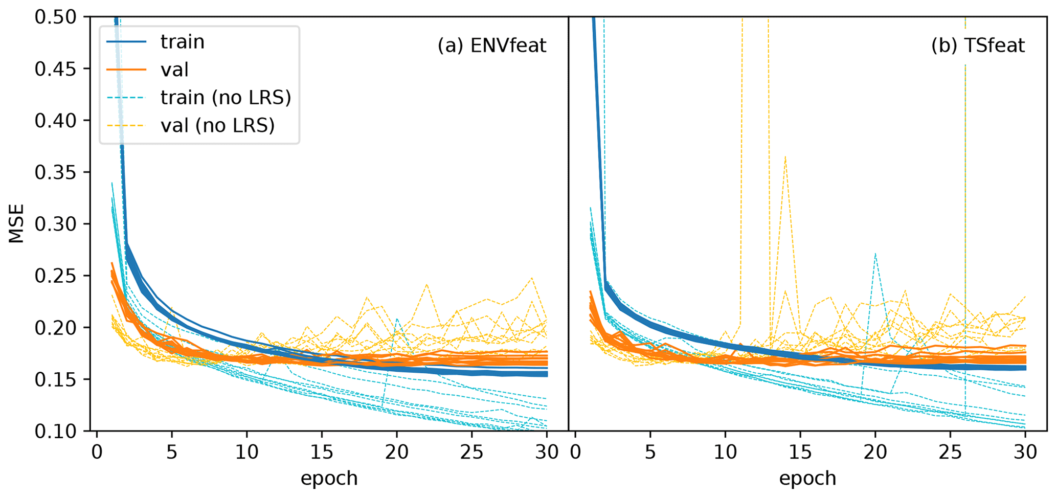
Figure 2 Loss curves of the training and validation period for the 10 different seed initialization runs for the (a) ENVfeat model and (b) TSfeat model, each with and without the learning rate scheduling described in Sect. 3.1. The figure shows a strong stabilization effect on loss curves.

Figure 2 shows the loss curves for 10 seeds with and without the LRS for the in-sample ENVfeat and TSfeat models (see Fig. A4 for loss curves of the other model variants). The TSfeat model does have a slight MSE improvement with a mean of 0.002 when using LRS, but the ENVfeat model actually performs slightly worse with a mean MSE decrease of 0.008 when using LRS. The same can be said when considering NSE in the test period, where mean performance decreases by 0.0005 with LRS. These changes in performance are negligibly small fluctuations around zero, and in essence, it can be said that model performance is basically the same with or without LRS. Thus, no greatly improved performance can be observed, as was achieved by, e.g. Smith and Topin (2018) and Li et al. (2019). However, introducing LRS comes with a strong stabilization effect on the loss curve (Fig. 2): While learning without LRS shows tendencies of rapid overfitting as well as of heavily exploding gradients, none of that is visible when using LRS. Loss curves with LRS are near-ideal, with train and validation loss curves approaching each other gently, and the validation loss curve never significantly increasing after reaching its minimum. The greatly increased stability of the loss curve implies much better generalization abilities of the model when applying LRS and shows the big advantage of this technique.

Figure 2 also shows some degree of bias in the validation dataset. This can be seen by the faster initial convergence of the validation loss curve. This is most likely due to the fact that validation data were not stratified, i.e. uniformly sampled over the whole period or frequency spectrum. Instead, we used the fixed period of 2008–2011 (and test period is 2012–2015, see Sect. 3.1). These periods constitute the most recent years, and were consciously chosen as fixed because the ultimate aim is forward prediction of groundwater levels, where the most recent groundwater levels are most representative for future predictions (as opposed of choosing rolling time periods for validation and testing).

3.3 Experimental design

After evaluating the effect of the LRS approach on training, we set up three different global model variants with static features. Using the model architecture described in Sect. 3.1, we either used static time-series features, static environmental features, or random static features in the static model thread to build the time-series feature model (TSfeat model), the environmental feature model (ENVfeat model), and the random feature model (RNDfeat model), respectively. The RNDmodel was run with two different numbers of features, i.e. 9 to be consistent with the number of features in the TSfeat model, and 18 as used in the ENVmodel. Additionally, we ran a ground-truthed model variant without any static features, i.e. only the dynamic strand (DYNonly model) as described in Sect. 3.1.

To test the performance of the models, we first run all models in an in-sample (IS) setting where all wells are used for training and performance is evaluated for each well separately based on the NSE score in the test period. We then compare their test score (NSE) with the results of the single-station models of Wunsch et al. (2022a), i.e. models trained and hyperparameter-optimized on every well separately. Importantly, we took their published results for this and did not rerun any of the single-station models. Also, it should be noted that comparing with the single-station scores of Wunsch et al. (2022a) is not benchmarking in a narrow sense, since some differences beyond the model architecture exist, e.g. Wunsch et al. (2022a) did not use RH as an input (which is used here) and optimized the input sequence length (which is fixed to 52 here).

To further test desired capabilities of spatial generalization, all global models were additionally run in an out-of-sample (OOS) setting, where the models are tested on unseen data, i.e. wells not used for training. Specifically, for every well the models are trained leaving the entire data of the wells out of training, and then predicting the score of the wells using only the their test data. Practically, this would equate to applying a leave-one-out (LOO) cross-validation, but due to computational constraints, we used 10-fold cross-validation instead to test the described OOS performance. To ensure robustness of the results, all models were run with 10 different seeds for random weight initialization on both settings (IS and OOS).

Finally, to understand the inner workings of the model, and how its performance relates to its input data, permutation feature importance (PFI, Fisher et al., 2019) was applied. PFI was chosen over alternative methods like SHAP (Lundberg and Lee, 2017) due to their high computational cost. With PFI, we measure the importance of features by successively taking every individual input feature (dynamic or static) of the trained model, permuting it by shuffling it randomly, and then calculating the model error (here: MSE) in the test data. A strong increase in the model error equates to a high importance of the feature being shuffled. This was repeated for each of the 10 randomized initialization seeds.

An additional side experiment was to compare the LSTM-based model with a modified version where the LSTM layer is replaced by a CNN layer, as suggested by the results of Wunsch et al. (2021b). However, the results of the CNN variants showed consistently lower performance in the model set-up used (see Fig. A1), and thus the results shown in the following focus on those of the LSTM models.

4 Results and discussion

4.1 Performance comparison of model variants

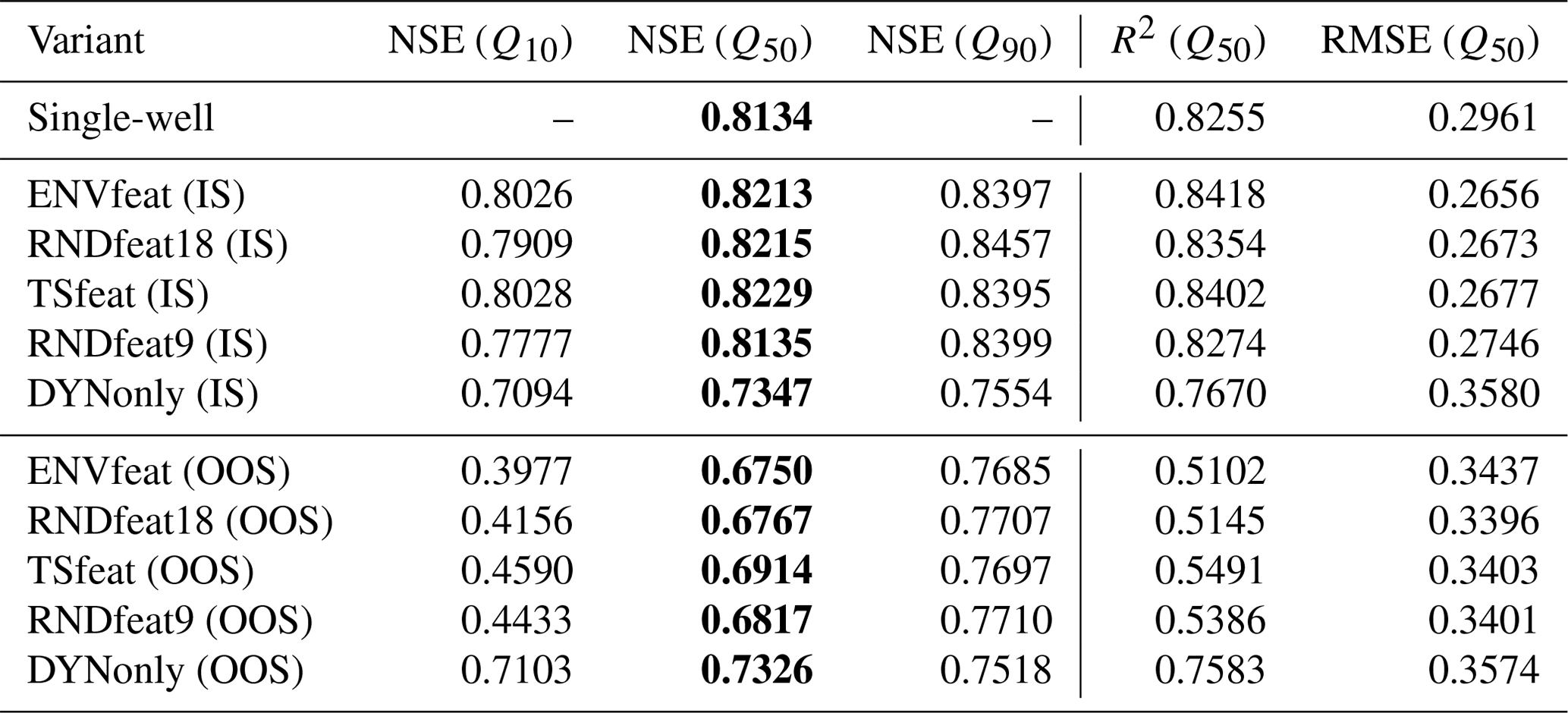
A side-by-side comparison of all global model scores and the single-well model scores of Wunsch et al. (2022a) can be seen in Fig. 3. The mean, lower (10 %), and upper (90 %) percentile NSE of the 10 ensemble members for all model variants are shown in Table 3.

In the IS validation, all global models with the exception of the DYNonly model perform almost identically with only minor differences, at the level of statistical noise. Only the RNDfeat9 model seems to show a slightly lower performance. Two things are somewhat unexpected in this result: first, that the TSmodel does not outperform the ENVmodel, and second and even more striking, that the RNDfeat models can keep up with the performance of the models with “meaningful” static features. This result corresponds to the findings of Li et al. (2022), who replaced their static environmental features with random counterparts and found similar or even improved performance for rainfall–runoff modelling in CAMELS basins. We speculate that the models use the static features solely as a kind of “unique identifier” for the wells; thus, it does not seem to matter if the static values represent some meaningful information (in terms of generalization) or not. This shows that our model is not able to learn from wells with similar static features, probably due to the number and choice of wells in the dataset considered. The reason for the inferior IS performance of the DYNonly model, however, seems obvious: since no static features are provided, the model is not able to distinguish between the different wells and instead fits to some average behaviour of all wells.

All global models with static features also slightly beat the scores of the single-well models. This result confirms observations by Kratzert et al. (2019a, b), who also observe better scores of global models over single-station models in rainfall–runoff prediction. These seemingly contradictory results – after all, single-well models are specifically optimized for the one specific location and should know this location best – is often attributed to the fact that, contrary to traditional hydrogeologic or hydrologic models, ML models benefit from additional data. However, with the RNDfeat models being as good as the TSfeat and ENVfeat models, we can widely exclude this as a reason in our case (maybe with the exception of the TSfeat model, which seems to perform slightly better than its RNDfeat9 counterpart). Benefiting from additional data or additional wells, respectively, would presuppose that the model is able to identify wells that react similar to meteorological inputs based on the static features provided. With the random number features being different for all wells and no meaningful similarity depicted in them, this cannot be the case.

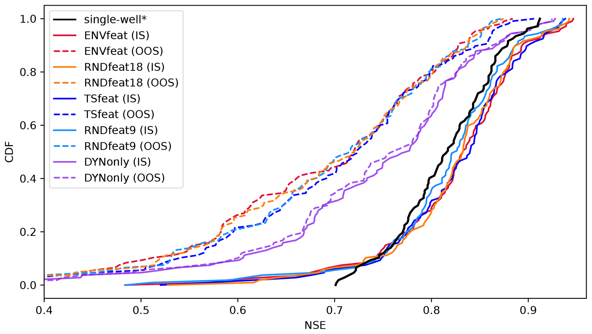
Figure 3 Cumulative distributions of NSE for the model variants ENVfeat, TSfeat, RNDfeat9, RNDfeat18, and DYNonly in in-sample mode (IS) and out-of-sample mode (OOS) against the performance of the single-well models by Wunsch et al. (2022a) (*). Lines represent sorted median NSE scores of 10 ensemble members. A version that includes the ensemble ranges as envelopes is shown in Fig. A5.

Table 3 Mean(bold font), lower (10 %) and upper (90 %) percentile NSE of the 10 ensemble members for all model variants as well as the mean NSE for single-well models (also in bold font) as published in Wunsch et al. (2022a). R² and RMSE show similar patterns to NSE and are reported for comparison, but not discussed in the text.

The differences to the single-well models might just as well be attributed to the different meteorological input parameters (RH and T_sin used additionally) and different optimization strategy. Moreover, despite being better on average, we observe a significant tailing in all global model set-ups, which the single-well models do not experience to the same degree (Fig. 3). The tail is the only part of the dataset where single-well models outperform both global models in 18 wells.

Figure 3 also shows the out-of-sample (OOS) performance of the global models, represented by 10-fold cross-validation runs. As expected, there is a sharp decrease in model performance when test data of a times series are predicted by a model that never saw the time-series training data. However, with a mean NSE of 0.675 (down from 0.8213, see Table 3) for the ENVfeat model, and a mean NSE of 0.6914 (down from 0.8229) for the TSfeat model, on average the OOS models perform surprisingly well, especially since some of the performance loss might be attributed to the compromise of 10-fold CV (instead of LOO CV), where about 10 % of possible training data are lost compared to the IS setting. These indications of model robustness are counteracted by the large seeding spread associated with both OOS models (Fig. 4 or A5), and an amplification of the tailing effect. Also, as in the IS case, the RNDfeat models perform nearly identically to the ENVfeat and the TSfeat models (Fig. 3), indicating that the model is not able to truly generalize well based on the static features provided, neither on the environmental nor on the time-series features. The TSfeat model performs at least slightly better than its RNDfeat9 counterpart, which could at least partly support our initial hypothesis that the TSfeat model would outperform the ENVfeat model since static time-series features are deemed to be informationally more complete and static environmental features suffer from high uncertainty. But the differences are minor and might be indistinguishable from noise due to the relatively low number of 10 ensemble members, showing a large range (Fig. 4 or A5). In the median, the ranges of NSE values at individual wells for different model seed realizations for the ENVfeat and TSfeat model are around 0.5 in the OOS setting, with minimum values of around 0.08 and maximum values of more than 1. Even though the spread is 1 magnitude smaller in the IS setting for all models (medians hovering around 0.05, see Fig. 4), this is a significant spread and shows that even if different model runs have the same NSE on the global level, they will have significantly different outcomes on the level of the individual well.

Most strikingly, the DYNonly model, having no static features at all, clearly outperforms all models with static features in the OOS setting (Fig. 3, Table 3). This indicates that the static features even seem to hamper the global entity-aware models from learning a meaningful relationship that is generalizable from the static features in the OOS setting. Furthermore, the OOS performance of the DYNonly model is as equally good as its IS performance (down to the third decimal, see Table 3), even though it relies on 10 % less training data. This implies information saturation, meaning that all information needed to reach the IS performance of the DYNonly model can be found in a significantly smaller subset of the dataset.

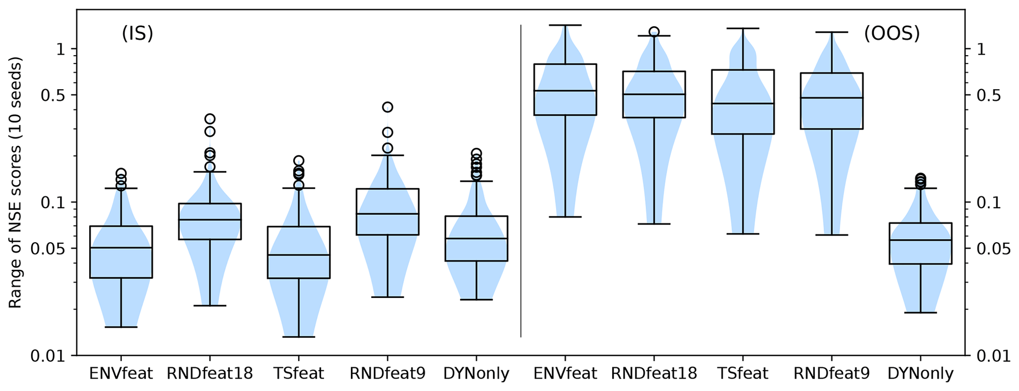
Figure 4 Range of NSE scores of the 10 ensemble members of all model variants in in-sample mode (IS) and out-of-sample mode (OOS).

More interesting insights can be drawn on the level of individual well predictions (Fig. 5, see the Supplement for all other wells). Basically, there are two groups of wells, where all wells show more or less the behaviour of one of the two groups, with smooth transitions in between. In the first group, exemplarily shown by well BB_30400591 (Fig. 5, top), the predictions in the IS setting of the ENVfeat, TSfeat, and RNDfeat models match rather well the observations with NSE for all models above 0.8, while the DYNonly model clearly fails (NSE = 0.169). Moreover, the predictions of the ENVfeat, TSfeat, and RNDfeat models are quite similar, confirming their overall similar performance. Thus, the models seem to obtain important information from the static features, that make it possible to better train the model to the individual behaviour of the well, while (as already postulated earlier) the kind of static information – environmental, time series, or random – does not seem to matter. On the other hand, the DYNonly model obviously lacks information about the special behaviour of the well, and probably predicts some average reactions to the inputs, which do not work well for the well considered. In the OOS setting, the predictions of all models are quite similar, or in other words, the predictions of the ENVfeat, TSfeat, and RNDfeat approach that of the DYNonly model, which is nearly the same as in the IS setting. The ENVfeat, TSfeat, and RNDfeat have obviously lost their ability to predict the individual behaviour of the considered well, as the well was not included in the training, and the model was obviously not able to generalize the relevant information from static data from other wells. Thus, there is a drastic drop in model performance between the IS and OOS setting. Other good representatives for this group are, e.g. well BW_107-666-2 and well SH_10L53126001 (see Supplement).

In the second group, represented by well SH_10L62060004 (Fig. 5, bottom), all model predictions in the IS and OOS setting, including the DYNonly model, are quite similar. All models perform well with NSE >0.8 and there is no obvious performance drop between IS and OOS. Our interpretation is that these wells show a more “average” behaviour in terms of their reaction to the meteorological inputs, i.e. the “average” reaction to the meteorological inputs that is learned by the DYNonly model. Therefore, the additional information provided by the static parameters does not improve model performance in the IS setting. Conversely, it also does not negatively influence model performance when this information is missing OOS, explaining the absent or minor drop in performance. Other good representatives for this group are, e.g. well BW_124-068-9 and well NI_200001722.

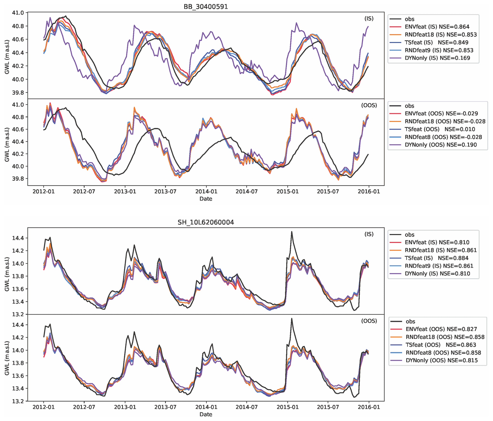
Figure 5 Examples of predictions of groundwater levels in the test period (2012–2015) for two wells, representing groups of similar behaviour (see text for details).

4.2 Permutation feature importance

By looking at the input feature importance of the models, further insights can be gained. We applied permutation feature importance to detect the relative importance of individual input features in the trained models. Figure 6 shows the feature importance of the ENVfeat, TSfeat, and RNDfeat models, separately for static and dynamic features (dynamic feature importance includes all model variants).

The first thing to note is that every individual dynamic feature is much more important than any of the static features, as the permuted MSE increase is higher by orders of magnitude for dynamic features. Thereby, as expected, precipitation and temperature are the most important features, followed by the sinus curve fitted to temperature. RH is least important. Even though there is some instability involved in these results, especially with T_sin and RH, but also P and T experiencing heavy outliers up to 2 magnitudes above the median, generally this confirms the findings of previous studies (Wunsch et al., 2021b). Admittedly, a more stable feature ranking could be obtained with alternative methods like SHAP (Lundberg and Lee, 2017), which was, however, not applied due to limited computational resources available to the authors.

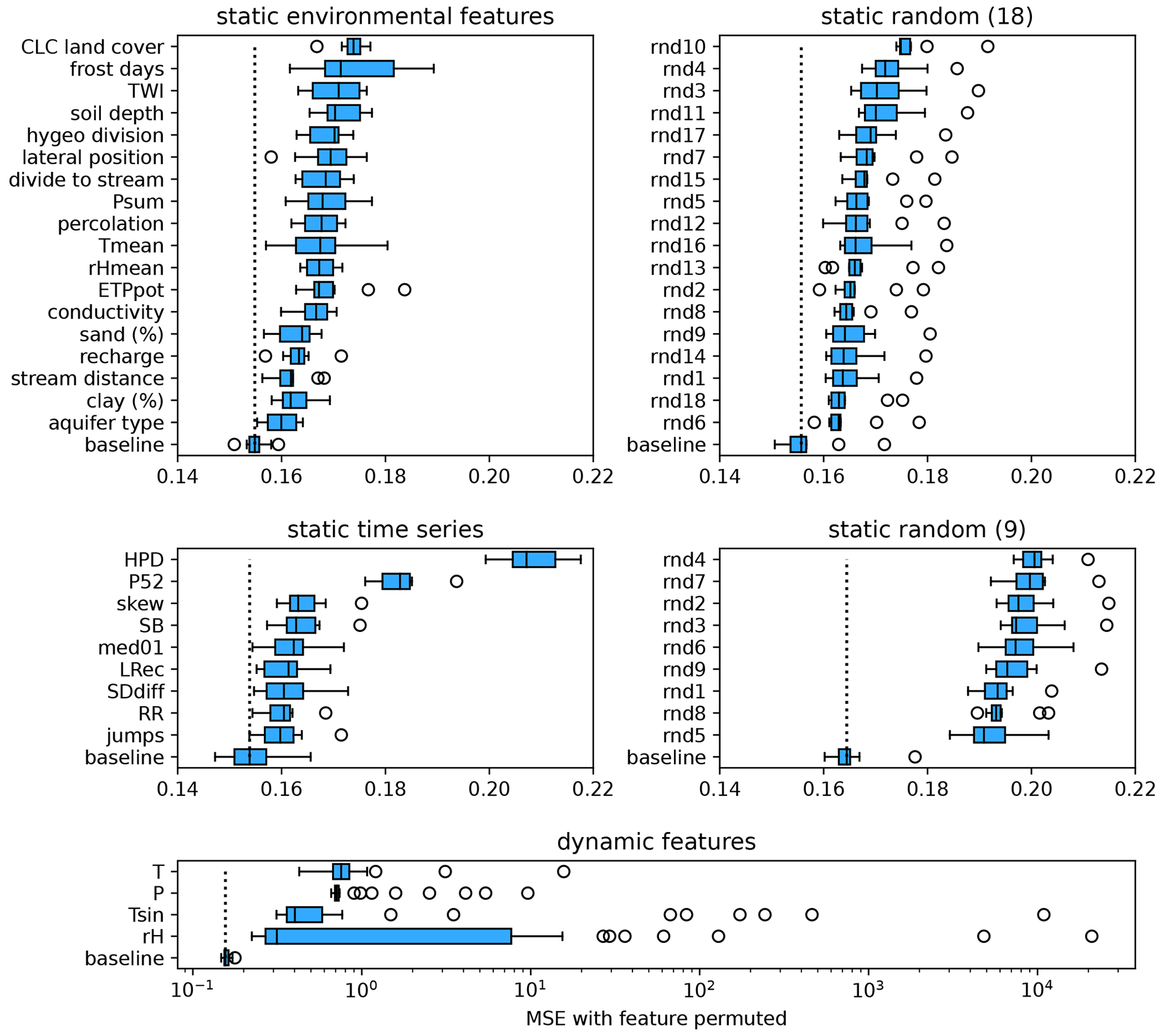
Figure 6 Permutation feature importance of the ENVfeat, TSfeat, and RNDfeat models, separately for static and dynamic features (dynamic feature importance includes all model variants). The dotted lines indicate the MSE of the baseline model, which includes all features. Larger deviations from this baseline indicate higher feature importance.

Among static features, we find much less difference between individual features (Fig. 6). Among static environmental features, CLC land cover comes out on top. This seems plausible because of its conceptual importance, and because it is the only feature representing land cover (although comprising 11 categories), unifying all information of land cover forcings, i.e. being informationally dense for the model. However, all environmental features show about the same feature importance as their random counterparts, confirming conclusions drawn in Sect. 4.1 that they do not contribute any meaningful and thus generalizable information to the model.

Static time-series features are somewhat more sensitive, with high pulse duration (HPD) and annual periodicity (P52) outpacing all other time-series features by some margin. But feature importance remains on a very low level for all other time-series features, which are even surpassed by the average (relative) importance of the nine random features, the exception being HPD. This allows the conclusion to be drawn that this is the only static feature that might provide some meaningful/generalizable information to the model. It also could be the reason that the TSfeat model at least slightly outperforms the RNDfeat9 model (compare Fig. 3).

In general, however, the most important finding to take from this result is the fact that all static features are orders of magnitude less important than the dynamic features, which implies that the model draws the majority of information used for prediction from the shared dynamic features. This can be used as an explanation for the finding that ENVfeat, TSfeat, and RNDfeat models perform almost identically (see Fig. 3), while DYNonly is able to outperform them in the OOS set-up.

5 Conclusions

The results of our work offer two main conclusions. First, in the IS setting, entity-aware global models work well and their performance can keep up with those of single-well models. All proposed model variants reached slightly better scores than the state-of-the-art single-station model. However, contrary to our initial hypothesis, the TSfeat model does not outperform the ENVfeat model. Moreover, the RNDfeat models – having random integers instead of “meaningful” static features – performed equally well as the TSfeat and ENVfeat variants. Against the backdrop of the IS DYNonly model (trained without static features, only on meteorologic input), which had severely reduced performance, it is evident that this is because all tested sets of static features appear to only act as unique identifiers, enabling the model to differentiate between time series and memorizing their unique behaviour, but not to establish meaningful system-characterizing relationships based on the static features. Thus, we conclude that the models do not learn adequately from wells with similar information as provided by the static features. It may not be worth the effort to gather supposedly meaningful data, since random numbers might work just as well (as long as a sufficient number of random features is provided). This finding is in accordance with studies that have been carried out in rainfall–runoff modelling (Li et al., 2022). Also, observed performance improvement over single-well models might just as well be due to architectural differences and the incorporation of additional dynamic input features (namely RH and T_sin) that were not considered in the published single-well model results used as comparison. In other words, the models introduced here perform better, but not necessarily for the reason of being global or entity-aware, according to the commonly made claim that global models profit from additional similar data.

Second, the OOS performance of all model variants with static features expectedly decreases significantly. In general this is still a respectable performance, making a case for good generalizability in principle. However, the DYNonly model significantly outperforms TSfeat, ENVfeat, and RNDfeat variants in this setting. This makes it evident that static features, acting as unique IS identifiers, obscure learning of the only true meaningful or causal connection, namely of dynamic (meteorologic) input features to OOS groundwater levels (i.e. when not included in training). In other words, the models are not able to learn that wells with a similar static feature combination should react similar to meteorological dynamic feature inputs in terms of groundwater level output. Instead, model skill is almost entirely based on learning from the dynamic input features. This might not come as a surprise for the environmental features, which were deemed to be afflicted with high uncertainties, but for the time-series features, since these proved in previous works to be well-suited to describe groundwater dynamics as a result of its reaction to meteorological inputs. Thus, our results suggest only a temporal generalizability potential – although valuable in itself – of entity-aware models, but lack evidence of true spatial generalizability potential – which remains the overarching aim of the field. However, this stands on the presented database, which, as already stated, might be too small, not diverse enough, and/or biased.

The tasks set by these conclusions are clear. First, since the dataset might simply not contain enough data to take full advantage of global models, we plan to investigate this with a larger dataset that covers groups of wells with several similarities as well as dissimilarities in a future study. The hypothesis is that when more wells with similar meaningful static information are included in the dataset, the entity-aware model might then be able to better learn and generalize from the provided features. Second, our study revealed the glaring research gap of finding and compiling meaningful environmental descriptors of groundwater dynamics with true predictive power. The hydrogeologic discipline lacks large-scale datasets of the kind. This severely restricts the development of hydrogeology as an ML research field, and the establishment of neural network models with physiographically meaningful internal structures, as was pursued in this study.

Appendix A

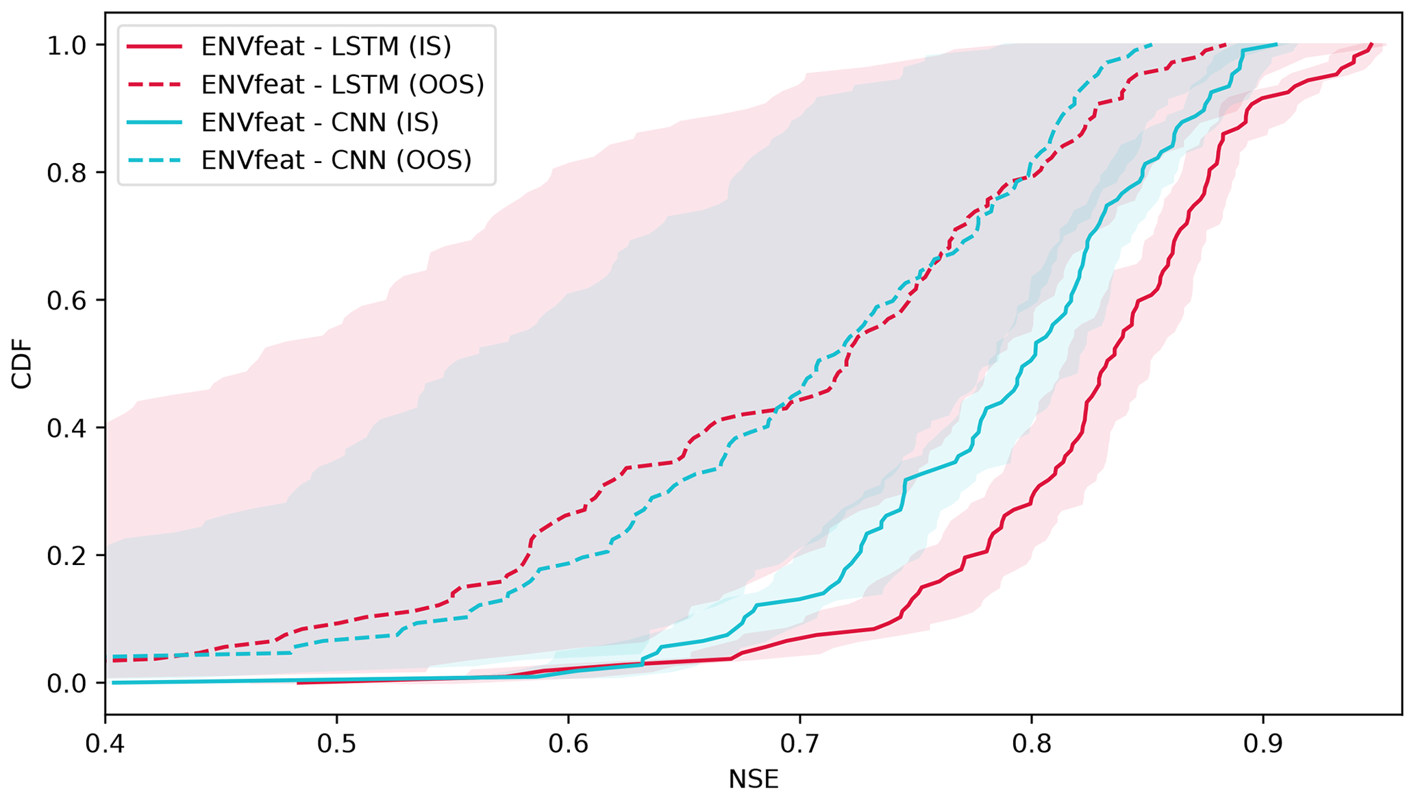
Figure A1 Comparing the performance of LSTM with CNN on the basis of the ENVfeat model variant. For the CNN model, the LSTM layer in the dynamic model thread is replaced with a CNN layer (followed by batchnorm and maxpool1D). The figure shows the performance of the models in an in-sample (IS) and out-of-sample (OOS) set-up. While CNNs and LSTMs perform almost the same in the OOS mode, CNNs are clearly inferior to LSTMs in the IS mode. Thus, LSTMs were used in this study.

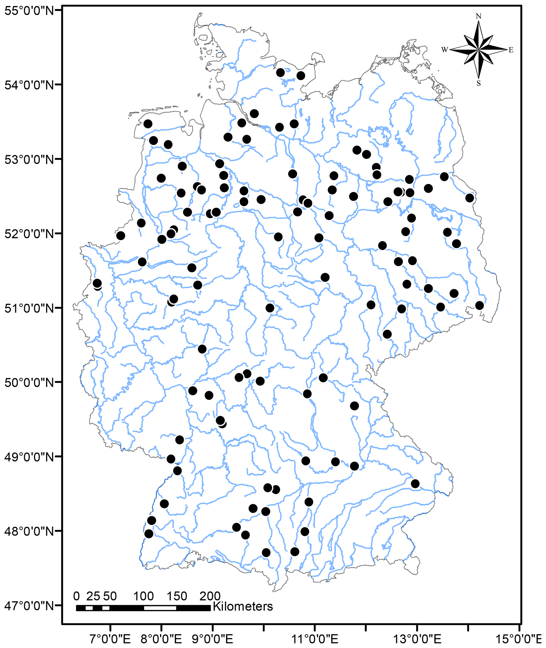
Figure A2 Location of the groundwater gauges in Germany.

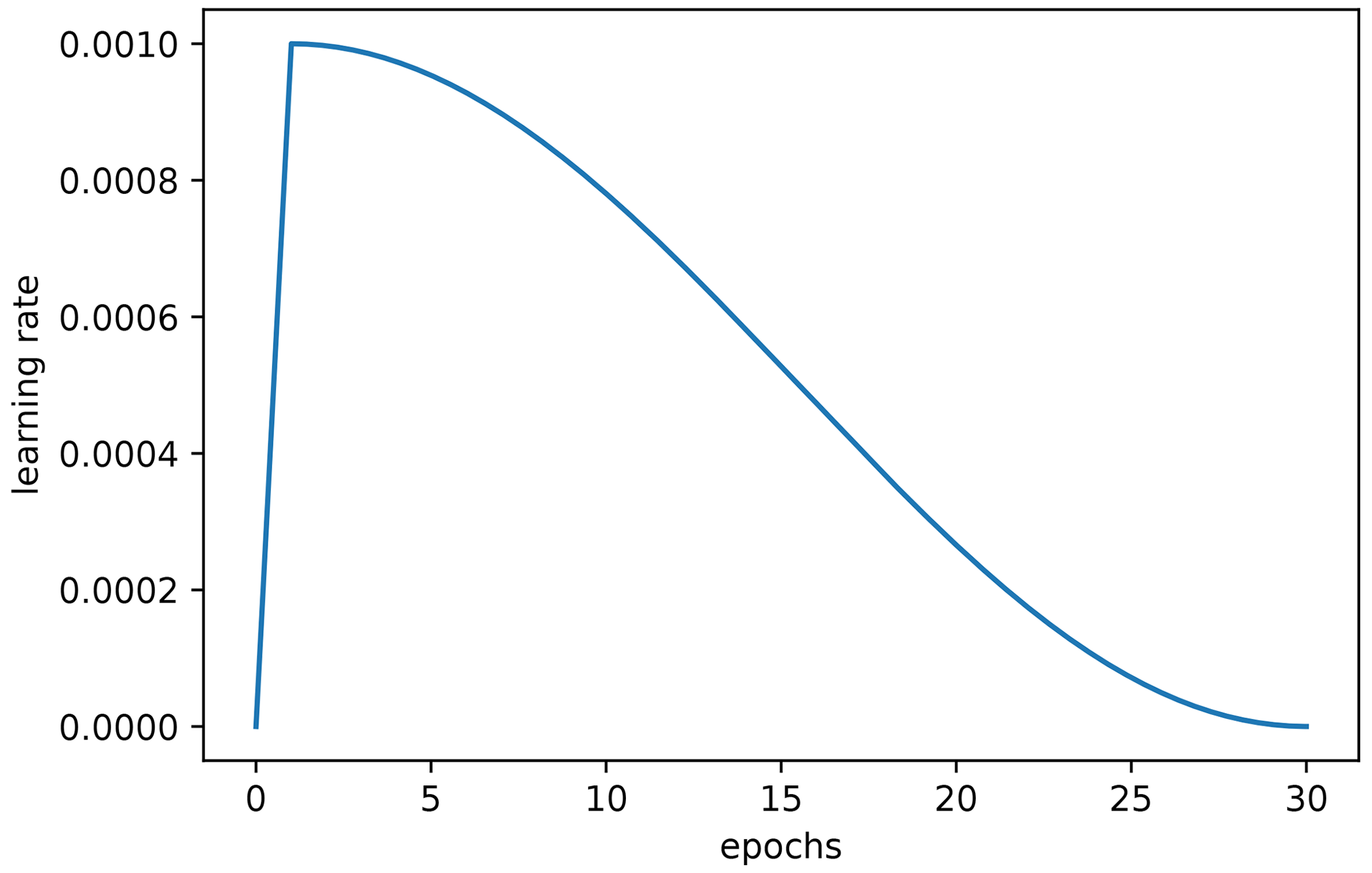
Figure A3 Visualization of the learning rate schedule used in this study. It consists of one warm-up epoch where the learning rate linearly increases from 0 to 0.001, followed by 29 epochs of cosine-shaped learning rate decline.

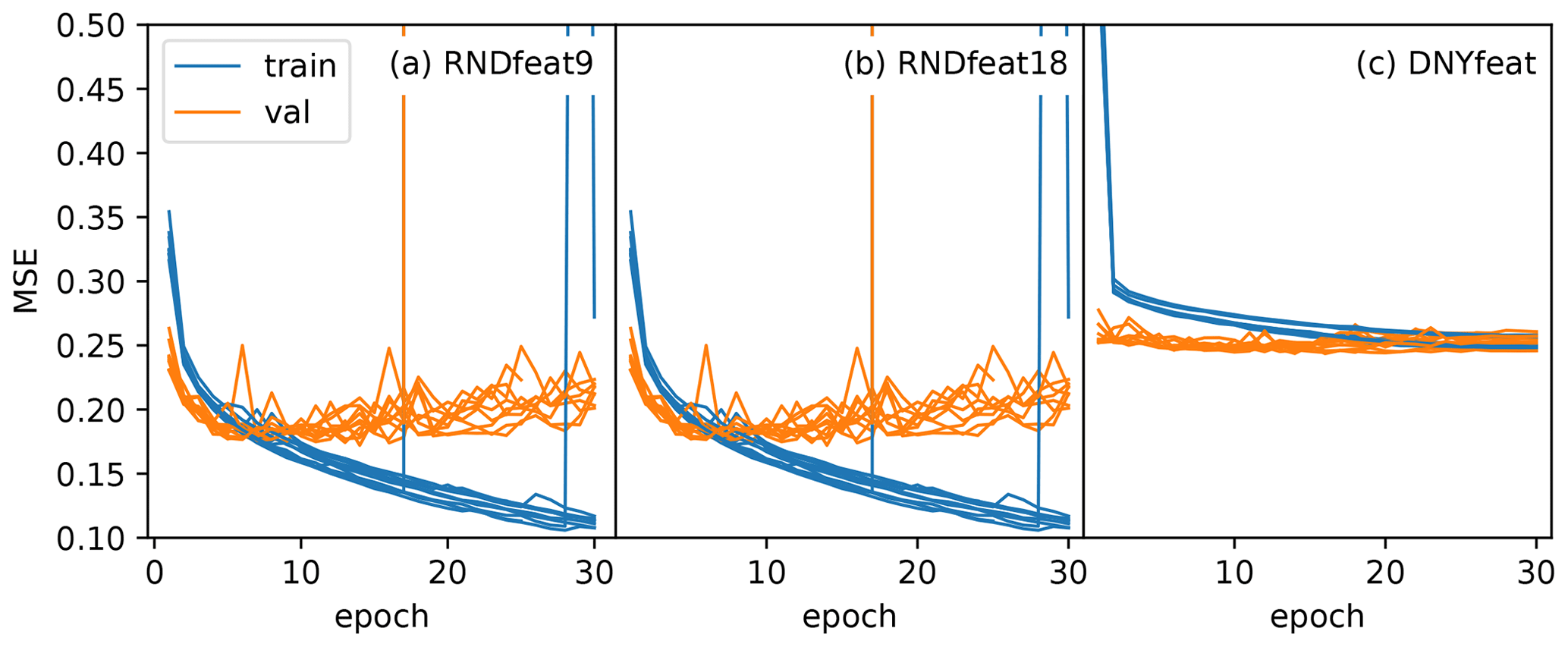
Figure A4 Loss curves of the training and validation period for the 10 different seed initialization runs for the (a) RNDfeat9 model, (b) RNDfeat18 model, and (c) DYNonly model.

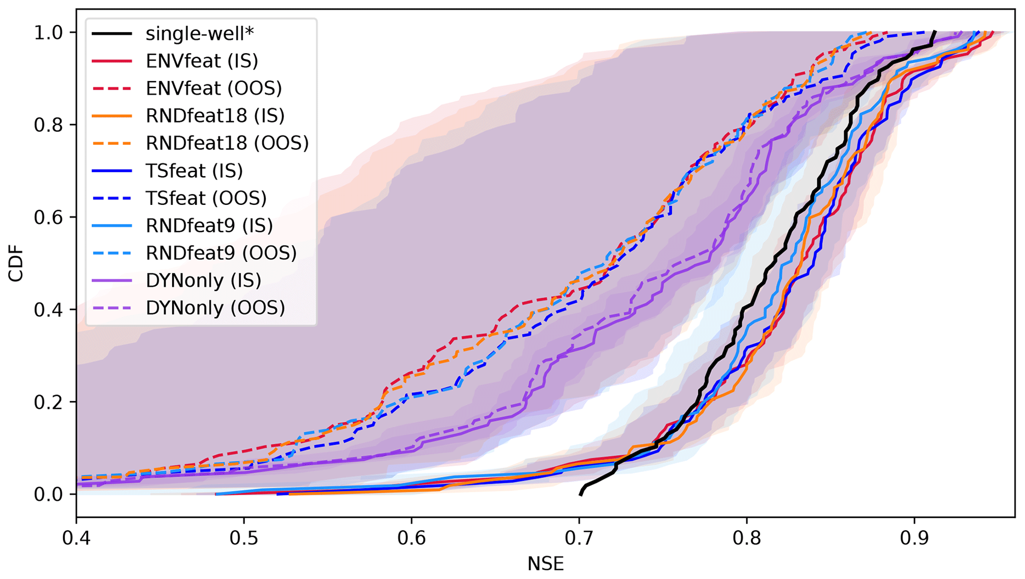
Figure A5 Cumulative distribution function of NSE of the model variants ENVfeat, TSfeat, RNDfeat, and DYNonly in in-sample mode (IS) and out-of-sample mode (OOS) against the performance of the single-well models by Wunsch et al. (2022a) (*). Lines represent sorted median NSE scores of 10 ensemble members, envelopes represent ranges of the ensemble forecasts excluding the worst and best member.