the Creative Commons Attribution 4.0 License.
the Creative Commons Attribution 4.0 License.
 | 07 Feb 2024
Incorporating interpretation uncertainties from deterministic 3D hydrostratigraphic models in groundwater models
Rasmus Bødker Madsen
Torben O. Sonnenborg
Lærke Therese Andersen
Peter B. E. Sandersen
Jacob Kidmose
Ingelise Møller
Thomas Mejer Hansen
Karsten Høgh Jensen
Anne-Sophie Høyer
Many 3D hydrostratigraphic models of the subsurface are interpreted as deterministic models, where an experienced modeler combines relevant geophysical and geological information with background geological knowledge. Depending on the quality of the information from the input data, the interpretation phase will typically be accompanied by an estimated qualitative interpretation uncertainty. Given the qualitative nature of uncertainty, it is difficult to propagate the uncertainty to groundwater models. In this study, a stochastic-simulation-based methodology to characterize interpretation uncertainty within a manual-interpretation-based layer model is applied in a groundwater modeling setting. Three scenarios with different levels of interpretation uncertainty are generated, and three locations representing different geological structures are analyzed in the models. The impact of interpretation uncertainty on predictions of capture zone area and median travel time is compared to the impact of parameter uncertainty in the groundwater model. The main result is that in areas with thick and large aquifers and low geological uncertainty, the impact of interpretation uncertainty is negligible compared to the hydrogeological parameterization, while it may introduce a significant contribution in areas with thinner and smaller aquifers with high geologic uncertainty. The influence of the interpretation uncertainties is thus dependent on the geological setting as well as the confidence of the interpreter. In areas with thick aquifers, this study confirms existing evidence that if the conceptual model is well defined, interpretation uncertainties within the conceptual model have limited impact on groundwater model predictions.
- Article
(5376 KB) - Full-text XML
-
Supplement
(659 KB) - BibTeX
- EndNote


Hydrostratigraphic models are the backbone of a groundwater model. They define the physical structure and the parameter zonation according to which the movement of water, storage and solute transport take place in the groundwater model. A hydrostratigraphic model is subject to uncertainty, and it is well known that it is a large source of uncertainty in groundwater model predictions (e.g., Huysmans and Dassargues, 2009; Moore and Doherty, 2005; Troldborg et al., 2007; Poeter and Anderson, 2005). Characterizing these uncertainties is important as it can provide decision-makers with information about the accuracy of model predictions, and this has been the subject of numerous studies (e.g., Barfod et al., 2018; Feyen and Caers, 2006; Li et al., 2016; Zhang et al., 2021).
Generally, hydrostratigraphic modeling can be divided into two main groups in which uncertainties are characterized differently: interpretation-based approaches and geostatistical approaches. In the interpretation-based approaches, a single deterministic geological or hydrostratigraphic model is constructed manually through the modeler's co-interpretation of all available data (e.g., Høyer et al., 2015; Jørgensen et al., 2013; Royse, 2010). The resulting model is viewed as the “best possible” representation of the subsurface given the available data and information. The main advantage of such a model is that it is directly based on expert knowledge, thereby ensuring geological realism. This has traditionally been the favored method for producing geological models. However, a common criticism is that both the final hydrostratigraphic model and the interpretation uncertainties are inherently subjective and biased in nature (Wellmann and Caumon, 2018). In contrast, it has also been argued that if a proper description of the subjective information is provided, the subjective element becomes a strength rather than a weakness (Curtis, 2012).
In geostatistical simulation approaches, multiple realizations are generated in order to represent a span of “equally possible” models of the subsurface (e.g., Høyer et al., 2017; Madsen et al., 2021; Mariethoz and Caers, 2015; Stafleu et al., 2011) and thus account for the inherent uncertainty of the geological model. Based on a set of assumptions, the equally possible models are generated automatically to represent the unstructured uncertainty within the conceptual model. Geostatistical simulations have been used in a number of studies to analyze the effects of combined geological and parameter uncertainty in relation to groundwater modeling (e.g., He et al., 2013; Refsgaard et al., 2012), just like other studies have focused on how the groundwater modeling can be optimized when simulating both hydrostratigraphic units and hydraulic conductivity uncertainty (e.g., Benoit et al., 2021). As the uncertainty modeling is already well established and a more natural consequence of geostatistical modeling, this paper aims at addressing the issue that the interpretation models lack a clear way to characterize uncertainties quantitatively.
In the interpretation-based geological models, a qualitative measure of uncertainty may be assigned to each interpretation point by the modeler. These uncertainties are based on several factors related both to the geological interpretation and the data (data type, resolution, density, and quality) (Høyer et al., 2023; Sandersen et al., 2018). Due to the qualitative and subjective nature of the uncertainty measure, which is related to the perceived uncertainty of the geologist when producing the deterministic interpretation model, this information has previously been lost and, hence, not incorporated in subsequent modeling, such as groundwater modeling. Thus, the uncertainties have only been discussed qualitatively when the purpose of the model requires it; for instance, in relation to landfill leachate risk assessment (Høyer et al., 2019) or groundwater vulnerability mapping (Hansen et al., 2016; Sandersen, 2008).
One attempt to consider the uncertainties of the manual interpretation models focus on the uncertainties related to the difference in conceptual geological understanding between different modelers. To consider this, some studies have engaged multiple teams of geological modelers to interpret the same data with an unknown conceptual model to come up with what they believe is the most likely model (e.g., Harrar et al., 2003; Hills and Wierenga, 1994; Refsgaard et al., 2006; Seifert et al., 2012). This approach is not widely applied as it is labor intensive and it is difficult to analyze the resulting uncertainty captured through the multiple models.
However, recently, approaches have been developed that transform the qualitative uncertainties of an interpretation-based hydrostratigraphic model into an ensemble of different realizations of the subsurface configuration through geostatistical simulation. In Troldborg et al. (2021), borehole interpretations were perturbed by assuming a normal distribution with a standard deviation reflecting a predefined groupwise uncertainty. Different sequential Gaussian simulation (SGS) realizations were generated by conditioning them on different perturbed borehole interpretations. The realizations were applied in an impact assessment of sheet piles on the water table. Further, Madsen et al. (2022) presented the geology-driven modeling approach, where a deterministic-interpretation-based hydrostratigraphic model can be transformed into a set of hydrostratigraphic realizations through SGS and interpretation uncertainties defined by the interpreter. The underlying probability distributions used in the SGS are inferred using a likelihood function, as opposed to the variogram-based modeling of Troldborg et al. (2021), which enables correlated effects of the interpretation uncertainty to be considered.
In this study, the method of Madsen et al. (2022) is implemented in a groundwater modeling context for an area in central Denmark. The interpretation-based hydrostratigraphic model is based on information from boreholes, airborne electromagnetic data and geoelectrical data (Enemark et al., 2022; Madsen et al., 2022). To our knowledge, the interpretation uncertainty for all layer boundaries in a manual-interpretation-based model has never been analyzed systematically in a groundwater model. Specifically, the influence of interpretation uncertainty on groundwater model predictions is evaluated in terms of the extent of the capture zones and the median travel times of water. The investigation is performed for three well fields in the study area that represent different geological structures and different levels of uncertainty. Three scenarios with diverse levels of uncertainty are investigated, ranging from an overconfident interpreter to a cautious one. Overconfident interpreters will generally assign low uncertainties to their interpretations, while the opposite is the case for cautious interpreters. Because the resulting groundwater models are affected by uncertainties in both the hydrostratigraphic and hydrological domains, the overall effect and significance of propagating the interpretation uncertainties are compared to uncertainties in the parameters of the groundwater model, such as hydraulic conductivity.
2.1 Hydrological and geological setting
The study area covers 127 km2 and is located just north of Horsens Fjord in Jutland, Denmark (Fig. 1). The catchment is delineated by a topography that ranges from 170 m above sea level (m a.s.l.) in the north to 0 m a.s.l. at the fjord. Approximately 2.7 M m3 yr−1 of groundwater are abstracted for drinking water from 20 different well fields within the study area. The groundwater system is restricted to the geological succession above the Paleogene clay, which is assumed to be impermeable and has a large thickness apart from areas where deep-buried valleys are eroded into the Paleogene clay. In parts of the model area, erosional remnants of Miocene sand, silt and clay exist on the plateaus, although the Paleogene clay is directly overlaid by Quaternary deposits in most of the area. The Quaternary succession is influenced by glacial erosion, and both glaciotectonics and multiple cross-cutting buried valleys have previously been mapped (Fig. 1; Jørgensen et al., 2010; Sandersen and Jørgensen, 2016). The Quaternary deposits consist of glacial and interglacial deposits of till, meltwater clay and sand, freshwater clay, sand and gyttja.
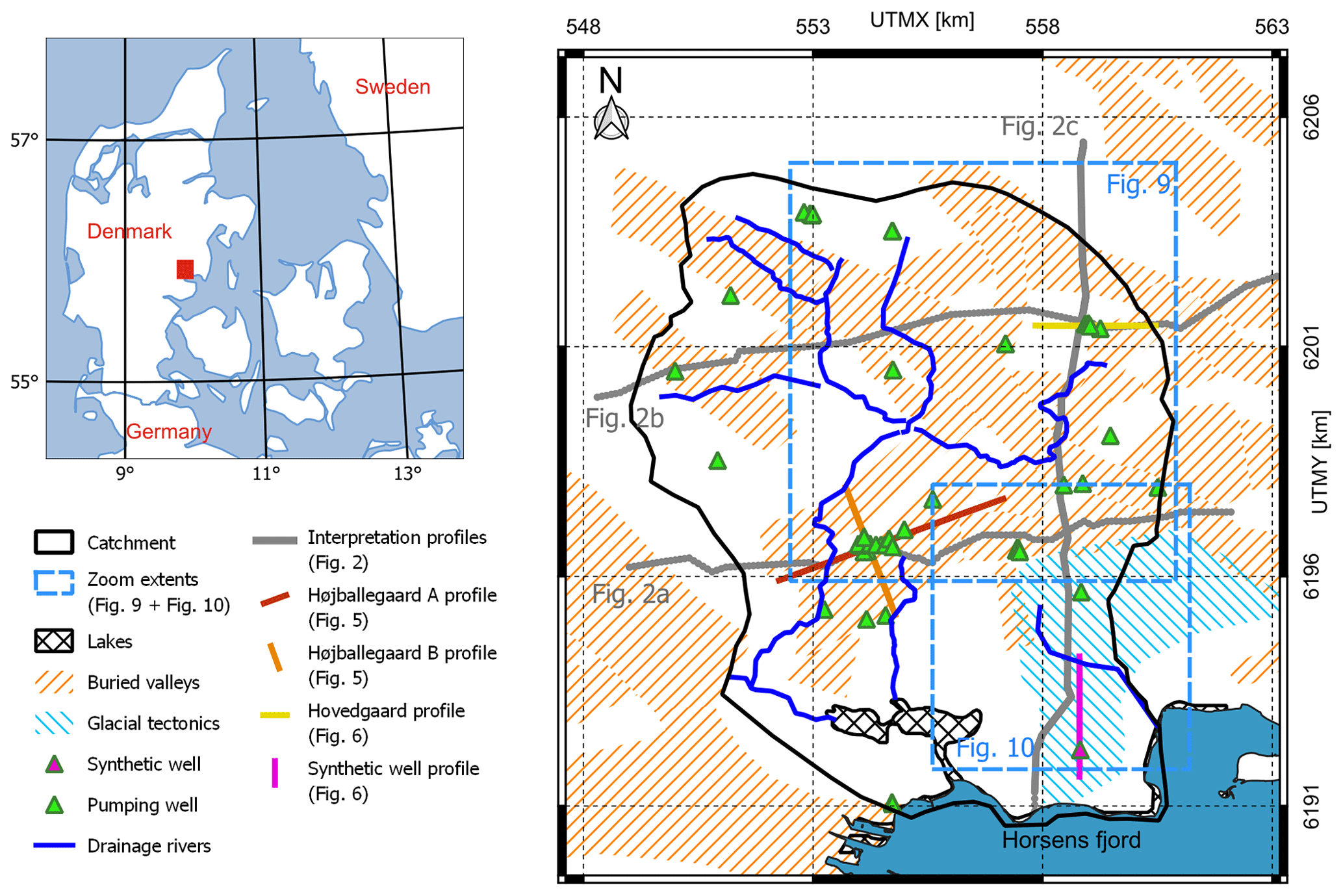
Figure 1Locations of the catchment, water abstraction wells, main rivers, glacial tectonics, buried valleys, profiles shown in Figs. 2, 5 and 6, and areas and zoom extents used in Figs. 9 and 10.
A deterministic and manually interpreted hydrostratigraphic model has been constructed for the area (Andersen and Sandersen, 2020), following the national guidelines described in Sandersen et al. (2018). The manual modeling is performed in the geological modeling software Geoscene3D (GeoScene3D, 2023) along a grid of fixed interpretation profiles placed such that they cross important geological structures and data. Three of these interpretation profiles are shown in Fig. 2. The figure shows the interpretation points together with the gridded layer surfaces and borehole data within a buffer of 50 m of the profile. Each of the layers in the manual model is constituted by a top and a bottom 2D surface.
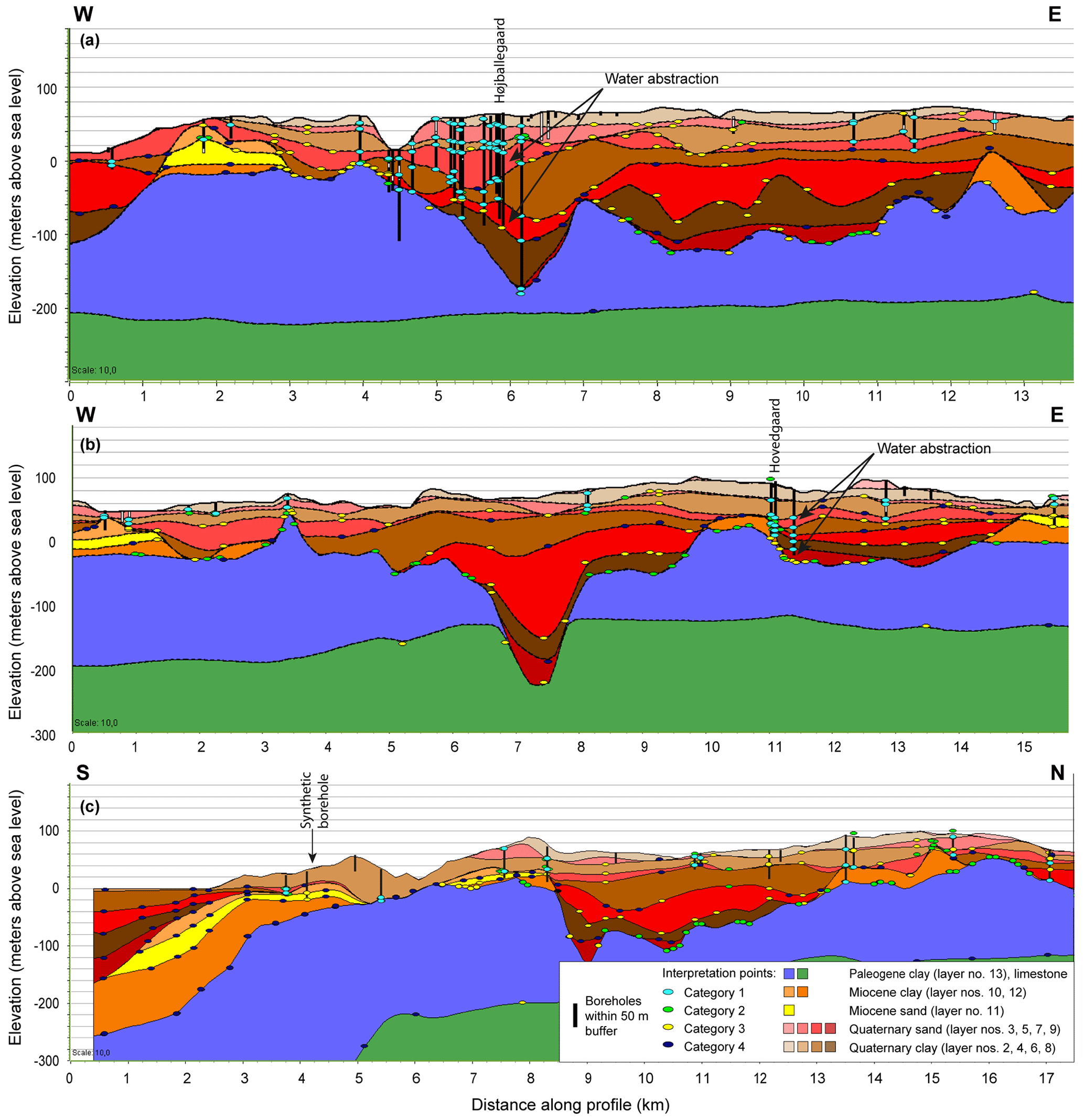
Figure 2Interpretation profiles through the catchment showing the manual interpretation model with interpretation points and their uncertainty categories. Interpretation points and boreholes within a buffer of 50 m from the profile are shown. (a) Interpretation profile crossing Højballegård well field. (b) Interpretation profile crossing Hovedgård well field. (c) Interpretation profile closest to the synthetic borehole (placed 900 m from the profile). The interpolated position of the borehole is marked at the profile. The locations of the profiles are shown in Fig. 1. The vertical exaggeration is 10×.
Interpretation points were manually placed along the interpretation profiles. The aim was an even spacing of a few hundred meters between points but a closer spacing in areas with marked variations. Subsequently, the layers were interpolated using kriging with adjusted semivariograms dedicated to each surface. To ensure that surfaces do not cross, they were adjusted using a dedicated tool in the modeling software after the gridding. The modeler set up rules of succession based on the erosional and depositional setting. Each interpretation point was attributed a qualitative uncertainty measure during the interpretation process, as shown with color-coded horizontal ovals in Fig. 2. The categories were defined as follows:
-
Category 1: points with the most certain interpretation; these are typically related to high-quality borehole information
-
Category 2: points for which the interpretation is certain; these are based on good-quality geophysical data and/or data obtained close to a borehole
-
Category 3: points with intermediate uncertainty; these are based on geophysical or borehole data of less good quality or ambiguous information
-
Category 4: uncertain information; this is based on the interpretation of data of poor quality, extrapolated data, or no data at all.
In the rest of this paper, the deterministic, manually generated, interpretation-based layered hydrostratigraphic model (Andersen and Sandersen, 2020) will be referred to as the manual interpretation model.
The manual interpretation model covers five pre-Quaternary layers and nine Quaternary layers. The pre-Quaternary layers consist of limestone, Paleogene clay, lower Miocene clay, Miocene sand, and upper Miocene clay. The Quaternary layers are divided into alternating clay and sand layers. The lowermost Quaternary layers are exclusively interpreted as valley infill deposits, whereas the upper Quaternary layers exist throughout the modeled area. The hydrostratigraphic model was constructed to focus on the hydrological properties of the deposits and does not distinguish between lithologies deposited in different geological environments, such as meltwater clay and clay till deposits.
2.2 Selected investigation sites
The study concentrates on two well fields in the area, Højballegård and Hovedgård, and a synthetic well field (see Fig. 1). The two real well fields (Højballegård and Hovedgård) were chosen because they represent different geological structures from which water is abstracted. The synthetic well field does not exist in the real world but was introduced into the analysis to represent an area with low data availability and thus a higher level of geological uncertainty. In the following, the geology and hydrostratigraphy of the three areas are summarized based on details described in previous studies (Andersen and Sandersen, 2020; Enemark et al., 2022; Madsen et al., 2022).
2.2.1 Højballegård well field
Højballegård well field, with 17 abstraction wells, is situated in the central part of the catchment (Fig. 1) and is the largest well field in the area, responsible for 87 % of the groundwater abstraction. The water is abstracted from a deep SW–NE-oriented buried valley structure that shows widths of up to 2 km and depths of up to 220 m. According to the borehole information, the valley infill deposits are relatively complex, with varying deposits of glacial origin, including meltwater sand, meltwater clay and clay till as well as thick occurrences of interglacial clay, sand and gyttja. In the manual interpretation model (Fig. 2a), the valley infill is divided into Quaternary sand and clay. The groundwater at Højballegård is abstracted from two different Quaternary sand layers (see the arrows in Fig. 2) separated by a clayey aquitard. In the model, the upper abstraction layer groups the meltwater sand deposited as valley infill and the Quaternary sand on the plateaus and can therefore serve as a hydraulic connection between the plateaus and the valley. The layer is laterally extensive (Fig. 2a, profile distance 2–8.5 km) and has a varying but usually substantial thickness (around 30 m at the well field). The lower abstraction layer is dedicated valley infill sand and is thus solely present in the buried valleys, with a thickness of about 40 m around the well field.
2.2.2 Hovedgård well field
Hovedgård well field is situated in the northeastern part of the catchment (Fig. 1) and is a small well field with four wells responsible for 3 % of the water abstraction in the area. The well field is located on the western flank of a SSW–NNE-oriented buried valley (Fig. 2b). The valley is up to 3 km wide but only 120 m deep. The valley infill at Hovedgård is less well described compared to Højballegård well field, with many lithological descriptions only indicating the lithology (sand or clay) rather than the depositional environment. According to the manual interpretation model (Fig. 2b), the valley infill is characterized by thin alternating layers of sand and clay. Water at Hovedgård well field is abstracted from deep sand layers (see the arrows in Fig. 2) modeled as valley infill. The abstraction layers are therefore restricted to the area of the buried valley and only locally present in the northern and southern parts of the valley.
2.2.3 Synthetic well field
To simulate the response of the models in an area with larger uncertainty, a synthetic well field was included in the southeastern part of the model area, with an appropriate distance to the boundaries of the groundwater model (Fig. 1). Here, the data are relatively sparse, and the interpretation points are generally assigned high uncertainties. In the groundwater model water is abstracted from the Miocene sand layer and is set to the same rate as for Hovedgård well field. At this location, the Miocene sand is interpreted to be relatively thin (10 m) (Fig. 2c). The Miocene layers are interpreted to dip towards the south due to the deep-seated fault structure in the southernmost part of the area.
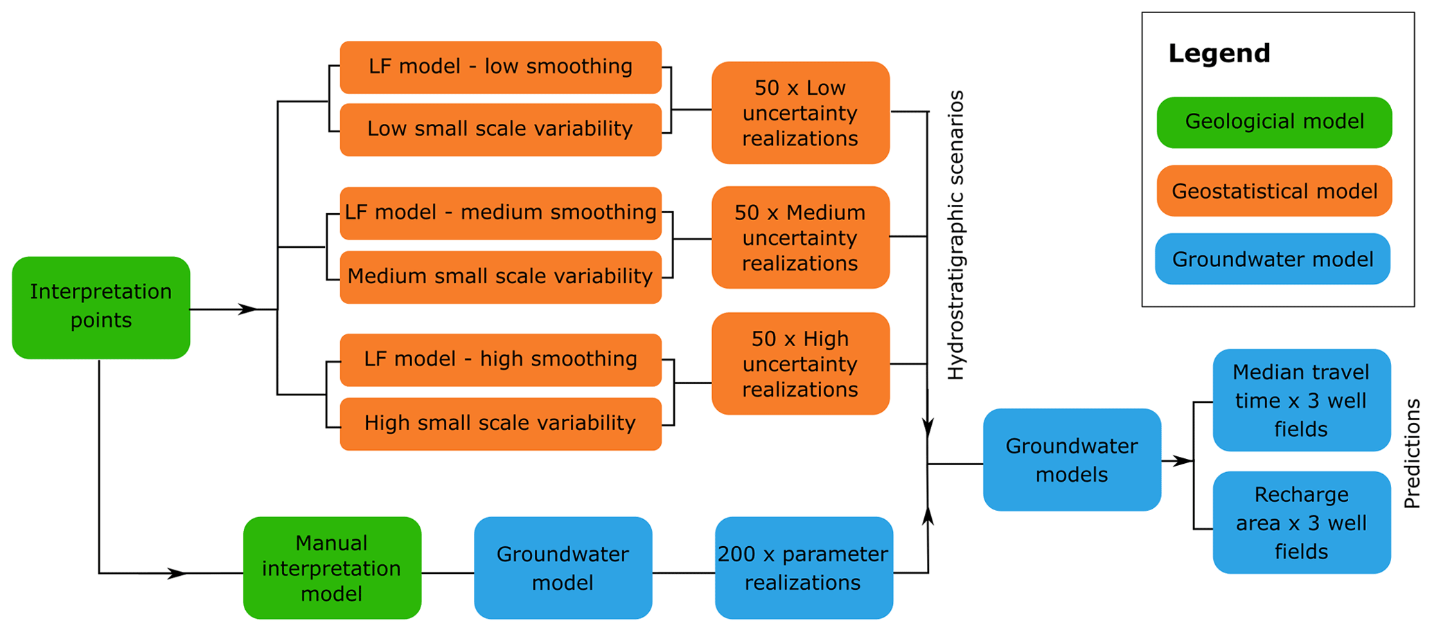
The workflow of the paper is summarized in Fig. 3. To evaluate the interpretation uncertainty of an initial interpreted hydrostratigraphic model, the hydrostratigraphic model is perturbed in three different uncertainty scenarios to produce 50 realizations in each scenario. In a groundwater model that uses the original interpreted hydrostratigraphic model, 200 parameter realizations are selected in a generalized likelihood uncertainty estimation (GLUE) approach. The 200 behavioral parameter sets are applied using the hydrostratigraphic realizations. In the following, a detailed description of the methodology is provided.
3.1 Hydrostratigraphic modeling
The geostatistical modeling described in Madsen et al. (2022, 2021) is based on the qualitative uncertainties evaluated at each interpretation point during manually interpreted hydrostratigraphic modeling (Andersen and Sandersen, 2020) (Sect. 2.1). To apply the methodology, the interpreter must provide (1) a quantitative estimate of the interpretation point uncertainty based on the qualitatively evaluated uncertainties and (2) a factor to balance the small-scale variability and large-scale structures (see Sect. 3.1.2). These preparational steps are described in the two following sections.
3.1.1 Point uncertainty estimates
In the applied methodology, each of the qualitative uncertainty categories is quantified using a Gaussian distribution, with the elevations of the interpretation points characterized by a mean and a standard deviation specified by the interpreter. The standard deviation for each uncertainty category is set to increase proportionally with depth and the resolution of the geoelectrical and electromagnetic inversion results. In layers with special properties where depth cannot be used as a direct proxy for uncertainty, an interpreted value is provided manually based on other information. For instance, the deep-lying Paleogene clay is well resolved with electromagnetic methods due to its low electrical resistivity, so it has low interpretation uncertainty in the manual interpretation model (see, e.g., Danielsen et al., 2003). However, it is essential to note that, even with this comparatively low interpretation uncertainty at the well-resolved boundary, the chosen uncertainty level should still reflect the uncertainties related to the processing and inversion of the geophysical data, especially as resolution decreases with depth (Madsen et al., 2022; Viezzoli et al., 2013). Specifically for geoelectrical models, the depth of investigation (DOI) can be introduced to help assess the validity of the geophysical model at depth (Christiansen and Auken, 2012). Below the DOI, it is appropriate to assign a high level of uncertainty, even for an apparently well-resolved layer such as the deep-lying Paleogene clay. Above the DOI, the quantification of standard deviations should factor in the resolution decrease of the inversion model with depth due to the increasing volume of subsurface that is being averaged over and the chosen regularization (Vignoli et al., 2015). Ideally, the standard deviation should also account for the possibility of inversion equivalences related to different parameterizations of the inversion scheme (Høyer et al., 2014).
3.1.2 Balancing small-scale variability and large-scale structures
The spatial variability between interpretation points is quantified by extracting (1) the large-scale structures of the interpretation points in a low-frequency (LF) model and (2) capturing the small-scale variability of the residuals with a Gaussian distribution. As Gaussian simulation rarely leads to a realistic geology (Journel and Zhang, 2006), this separation of the point information is introduced in order to improve the geological realism of the stochastic hydrostratigraphy by keeping the main geological features intact. In the current setup, the LF model is obtained by performing linear interpolation between interpretation points and then applying a smoothing kernel via a sliding window approach on the interpolated grid. To provide a balance between the small-scale variability and large-scale structures, the interpreter must provide a factor ε determining the width of a smoothing kernel used to construct the LF model. Figure 4 illustrates the structural input provided in the LF model. In one extreme, the interpretation model is used directly without applying any smoothing (Fig. 4a), giving all structural weight to the interpretation model. In the other extreme, the interpretation model is smoothed such that the LF content merely becomes the average depths of the layers providing the maximal weight to the small-scale variability (Fig. 4c).
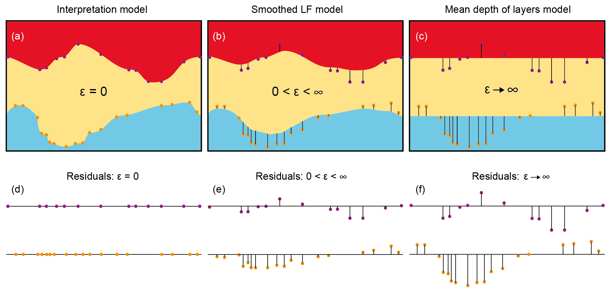
Figure 4Schematic overview of the effect of applying smoothing to a three-layer interpretation model based on interpretation points to obtain the overall structures in an LF model. (a) The interpretation model has no smoothing (ε = 0). (b) The interpretation model is smoothed (). (c) The interpretation model is smoothed to a degree that only represents the expected average depth of each layer (ε→∞). The resulting residuals for each scenario are shown underneath in (d–f).
As the significance of geological features varies across the modeling domain, the kernel width ε, and hence the level of smoothing, also varies at different locations. The modeler only provides the base level ε and the kernel width is then scaled according to the principle of locally assessing the changes in surface elevations. In a layer-based model, significant geological characteristics can correspond to sudden shifts in interpretation point elevations. These shifts will not arise through interpolation unless specific interpretation points are strategically positioned to guide the surface behavior accordingly. Thus, sudden shifts in interpretation point elevations are a good proxy for geological features that are worth extracting in the LF model. The variance amongst the interpretation points within the sliding window is calculated for the entire surface. If the variance is high, then the modeler has tried to convey large changes in the elevation and the smoothing becomes low to allow the LF model to follow these structures. In the other case, a low variance of elevation amongst the points within the sliding window leads to more smoothing of the LF model. In many places with a low variance in elevation, high uncertainty is attributed to the interpretation points by the modeler. We attribute this apparent correlation to the fact that a modeler would likely be unwilling to make bold structural interpretations in areas where there are no data to support such claims. Thus, the LF model will indirectly carry less information in areas with high uncertainty, which is desirable, although the LF model is based on the spatial structure of the interpretation points and not the uncertainty attributed to them.
Once an LF model is established, a statistical model for the small-scale variability is inferred from the residuals such that a set of realizations of each boundary can be simulated using the quantified spatial variability instead of being interpolated (as in traditional modeling). Ultimately, it is up to the modeler to choose a suitable smoothing that keeps important structural input in the LF model but allows for the desired spatial variability to be mapped in the residuals (Fig. 4b and e).
3.1.3 Uncertainty scenarios
In this study, three uncertainty scenarios are developed with different point uncertainty quantifications, each consisting of 50 realizations of the subsurface. Furthermore, the manual interpretation model does not serve as the ground truth; it can be thought of as one possible representation of the subsurface. Thus, the trust in the large-scale structures of the interpretation model is also varied between the three scenarios by varying the applied smoothing factor ε.
First, the uncertainty configuration of Madsen et al. (2022) is adopted as the medium uncertainty scenario, where ε= 700 m. Second, a low uncertainty scenario representing an overconfident interpreter is introduced. To emulate this, all interpretation uncertainties at point scale are reduced by a factor of 3 compared to the medium scenario, and the smoothing factor ε is subsequently decreased by 500 m to ε= 200 m, thus making the LF model very similar to the interpretation model. Finally, an insecure interpreter that estimates a high degree of uncertainty in his or her interpretations is introduced. The standard deviations at point scale of the high scenario are scaled up by a factor of 3, while the smoothing factor ε is increased by 500 m to ε= 1200 m to make sure that layers can deviate substantially from the manual interpretation model. The standard variations assigned to the different uncertainty scenarios are illustrated in Sect. S3 in the Supplement.
3.2 Groundwater modeling
Applying the same setup as in Enemark et al. (2022), steady-state MODFLOW-NWT (Niswonger et al., 2011) models are developed using the Flopy platform (Bakker et al., 2016). Two outputs of the groundwater model are evaluated: the extent of the capture zones and the median travel times of water particles from the water table to the well screen. These predictions are chosen, as they are not part of the calibration but will be affected by the calibrated parameter zonation. The discretization, boundary conditions and parameterization of the groundwater are described in the following.
3.2.1 Discretization
The horizontal discretization is specified as 100 m by 100 m, while the vertical discretization is based on the vertical extent of the hydrostratigraphic units from 165 to −250 m a.s.l.; i.e., each hydrostratigraphic realization has a distinct model grid. By grouping together three plateau sand units, two plateau clay units, two sand units in the buried valleys and two clay units in the buried valleys, we get eight hydrostratigraphic units in the groundwater model. The grouped units have the same or similar lithological descriptions as in the manual interpretation model but differ in their position in the geological sequence. The hydrostratigraphic units are parameterized by horizontal hydraulic conductivity, vertical anisotropy and porosity.
3.2.2 Boundary conditions
Using MODFLOW's Recharge (RCH) package, the recharge to the water table is represented as a diffusive source – a specified flux distributed over the top of the model. The well abstraction in the model is represented by the Well (WEL) specified flux package. In all models, regardless of the geometry of the model grid, the wells are set in the same layer to ensure model predictions can be compared; i.e., the depths of the 210 abstraction wells may vary between realizations, but the layer and therefore the lithology will be the same in all models. The lakes and fjord in the southern part of the model area are represented by the General Head Boundary (GHB) head-dependent flux boundary package. To simulate inflows to streams as well as subsurface tile drains and smaller ditches, the Drain (DRN) head-dependent flux boundary package is applied. The flux to the river cells is used as a calibration target.
3.2.3 Parameterization
Realizations of the parameterization to be used for the individual hydrostratigraphic realizations are generated by Latin hypercube sampling of parameter values within specified ranges. Five parameters and their prior parameter ranges, which are sampled, are presented in Table 1. A differentiation between buried valley sand and clay and plateau sand and clay is introduced, as the buried valley and plateau sediments may have different hydrogeological properties. Uniform distributions described by a minimum and a maximum value are applied, representing prior information on the parameter values. As the sampled parameters range over several orders of magnitude, the sampling was performed from log-uniform distributions. The remaining parameters are not subject to sampling and thus have fixed values, as they were shown to be insensitive in initial runs of the manual interpretation model.
Table 1Parameter value ranges and distributions used in the manual interpretation groundwater models. “Kh” refers to the horizontal hydraulic conductivity, while “cond” refers to conductance.
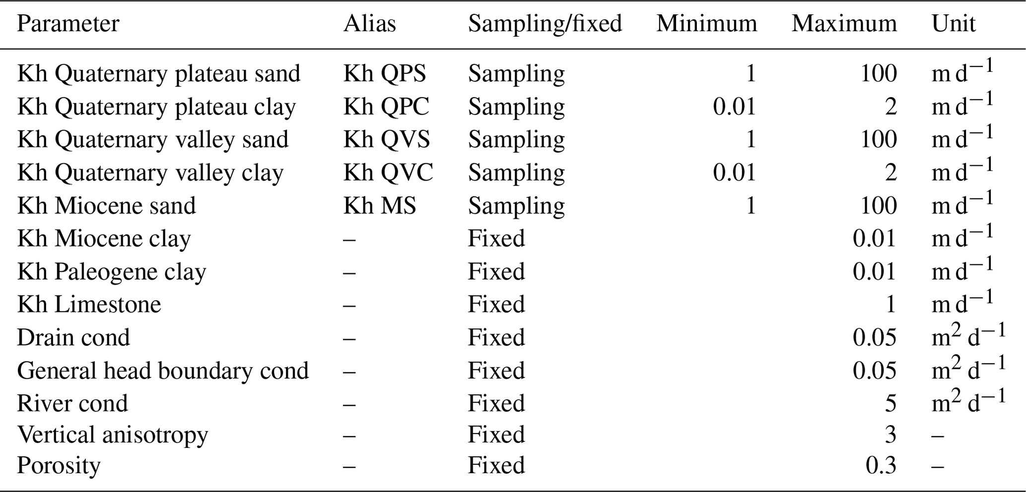
To obtain a range of posterior parameter sets, a generalized likelihood uncertainty estimation (GLUE) approach (Beven and Binley, 1992) is applied. Applying this approach, a subset of parameter sets that satisfy a set of predefined constraints simultaneously is obtained. Using the manual interpretation model, 10 000 realizations are run based on the prior parameter ranges presented in Table 1. Of these simulations, 200 parameter sets are retained according to the criteria below. Initial model runs in the manual interpretation model showed that the predictions of interest – the capture zone area and travel time – do not change significantly after 200 model runs (Sect. S1 in the Supplement). Thresholds for selected performance metrics based on values in the Danish groundwater modeling guideline (Henriksen et al., 2017) are applied. The following thresholds are applied: 0.9 m for the mean error of hydraulic heads, 5 % for the river observation error, and 9 m for the root mean square error of hydraulic heads. Initial model runs showed that the same parameter values in different uncertainty scenarios attained similar performance. Therefore, these parameter sets were then applied to the other uncertainty scenarios. The posterior parameter distributions are presented Sect. S2 in the Supplement.
3.2.4 Particle tracking
Particle tracking simulations are performed using MODPATH 6 (Pollock, 2012). In each topmost active cell, 10 particles are tracked forward to discharge points, and the particles that are discharged into the well fields of interest (Sect. 2.2) are extracted. Initial simulations in Enemark et al. (2022) showed that the capture zone area stabilizes when around 10 particles are inserted into the upper cells of the layer model in a layer grid. Only particles with a travel time of less than 200 years are retained, as 200 years is the typical value for determining capture zone areas in Denmark (Iversen et al., 2009).
4.1 Hydrostratigraphic model
The quantified boundary uncertainties in four cross sections around the three well fields are illustrated in Figs. 5 and 6. The topmost profiles (Figs. 5a, e and 6a, e) show the cross sections through the manual interpretation model. The three profiles below illustrate the boundary uncertainties in the low, medium and high uncertainty scenarios in terms of mode and entropy. The mode represents the most probable value, while the entropy is a measure of the uncertainty associated with the mode. In Figs. 5 and 6, the mode is represented by the boundaries where the color changes, and the entropy is superimposed such that the colors become increasingly transparent when the entropy is high (i.e., the uncertainty is high) and, conversely, the true color is present when the entropy is zero. Overall, the large differences in interpretation uncertainty between the three uncertainty scenarios manifest as increasingly thick zones of uncertainty around the boundaries upon going from the low to the medium to the high uncertainty scenario (e.g., the black ellipses in Fig. 6b–d). The overall conceptual model consists of a thick base of impermeable Paleogene clay and alternating layers of Quaternary clay and sand situated on top and is preserved in all scenarios. If either of these mode models were to be presented as the sole model to be used for groundwater modeling, it would be hard to dismiss it as being any less true or useful than the manual interpretation model. Thus, the important overall structures carried over from the LF model are considered a fair representation of the overall geology, while the interpretation uncertainty at the boundaries is showcased by the entropy.
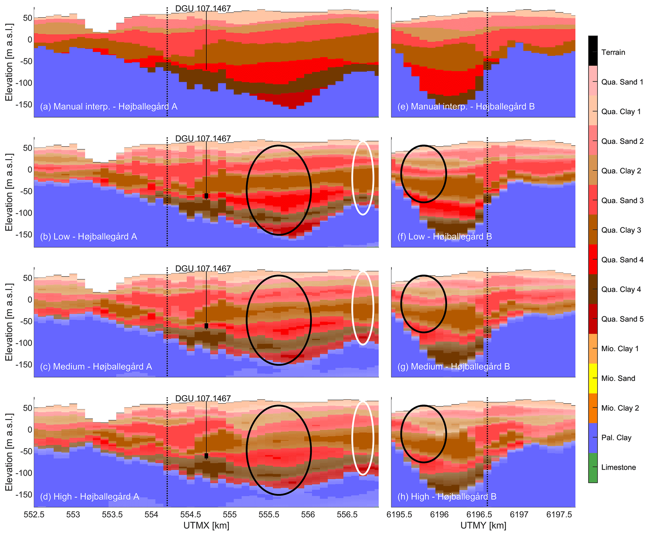
Figure 5Two intersecting cross sections of summary statistics for the hydrostratigraphic model realizations: Højballegård A (a–d) and Højballegård B (e–h). The locations of the cross sections can be seen in Fig. 1. The intersection between the cross sections is marked with dotted lines. Abstraction boreholes from the well field are marked with a solid black line, and the inlet filters are marked with a black rectangle. The colors become increasingly transparent when the entropy is high. (b, f) Summary statistics from the low uncertainty scenario, (c, g) summary statistics from the medium uncertainty scenario, and (d, h) summary statistics from the high uncertainty scenario. The black ellipses are examples allowing a comparison of the boundary uncertainties in the three scenarios, and the white ellipse shows an example of how borehole information lowers the uncertainty at the boundaries.

Figure 6Two cross sections of summary statistics for the hydrostratigraphic model realizations at Hovedgård (a–d) and the synthetic well field (e–h). The locations of the profiles can be seen in Fig. 1. Abstraction boreholes from the well fields are marked with a black line, and the inlet filters are marked with black rectangles. Note that the filter is missing from the cross sections at the synthetic borehole as it is not fixed in space but placed in the Miocene sand during groundwater modeling. The colors become increasingly transparent when the entropy is high. (b, f) Summary statistics from the low uncertainty scenario, (c, g) summary statistics from the medium uncertainty scenario, and (d, h) summary statistics from the high uncertainty scenario. The black ellipses are examples allowing a comparison of the boundary uncertainties in the three scenarios.
In the real well fields (Højballegård and Hovedgård; Figs. 5 and 6a–d), where the abundance of data and interpretation points is high, the difference in entropy is larger between the low and medium scenarios than between the medium and high scenarios. This can be attributed to the lack of spatial freedom of the layer boundaries, which are naturally constrained by the sheer number of interpretation points. In contrast, when the number of interpretation points is small, as is the case around the synthetic well field (Fig. 6d–f), increasing or decreasing the uncertainty level has a significant impact on the resulting hydrostratigraphic realizations.
A slight change in mode can be observed between the three uncertainty scenarios (Figs. 5 and 6), which is a result of changing the smoothing in the LF model, reflecting a lower information level. This difference is apparent in regions with a low density of interpretation points, where the model may deviate significantly from the manual interpretation model. For example, in Fig. 6h, the average depiction of Quaternary sand deposits (red colors) is higher compared to Fig. 6f–g. However, in areas with high interpretation point density, as seen around the well in Fig. 5b–h, each uncertainty scenario has a similar mode model.
In general, borehole information (for which the uncertainty is rather low in all three scenarios) is easily identified for all three scenarios as vertical parts of the probabilistic model that are associated with low uncertainties near the layer boundaries of the model (e.g., the white ellipse in Fig. 5b–d). Despite the lowered uncertainty in these vertical sections, the trend of a varying uncertainty between the scenarios can also be spotted at these locations. All the above-mentioned observations are in accordance with expectations regarding the behavior of the model for the three uncertainty scenarios.
4.2 Groundwater model
In each of the three hydrostratigraphic uncertainty scenarios, the 50 hydrostratigraphic realizations are run with the same 200 groundwater parameter realizations in the groundwater model. In the following, the results of the groundwater models are presented. In the low, medium and high uncertainty scenarios, respectively, 7 %, 4 % and 3 % of the realizations did not converge and are therefore not included in the analysis. In Sect. 4.1 it was observed that the realizations of the low uncertainty scenario are not necessarily more like that of the original manual interpretation model than the realizations of the high uncertainty scenario, which may explain the difference in the convergence rates. The convergence rate is likely influenced by the model grid (which is unique for each realization), as it follows the layer elevations. The model grid is thereby influenced by the smoothing of the hydrostratigraphic model (Fig. 3). The low smoothing of the low uncertainty scenario allows larger changes in layer elevations than the high smoothing in the high uncertainty scenario does. In areas where the layers are thin, this may result in a lack of lateral continuity between adjacent cells, which causes an inability to simulate flow between cells in the same layer. Further, at the synthetic well field, the water table falls below the screen top in 46 %, 6 % and 1 % of the realizations, respectively, in the low, medium and high uncertainty scenarios, which we will elaborate on in Sect. 4.2.5. These realizations are excluded from further analyses.
4.2.1 Ensemble performance
The performance of the model realizations in the three uncertainty scenarios is shown in Fig. 7. The evaluated performance metrics consist of the root mean square error (RMS) and mean error (ME) of the hydraulic head and the river flow error. The gray area illustrates ranges for the performance metrics that are beyond the threshold values. In the manual interpretation model, thresholds have been applied directly to the performance metrics. In the other uncertainty scenarios, the same parameters retained from the manual interpretation model have been applied. For each performance metric, the range covered by the manual interpretation model is therefore the lowest, while it increases with the level of uncertainty introduced into the uncertainty scenario. It is shown that almost 90 % of the realizations (between the 5th and 95th percentiles) are within the threshold values for the low and medium scenarios, while this percentage is a bit less for the high uncertainty scenario. Therefore, the uncertainty associated with assuming that the same parameter sets are applicable for the other hydrostratigraphic realizations is illustrated. The simulations from the high uncertainty scenario have larger ranges of variation for all performance criteria, while the simulations from the low uncertainty scenario have smaller variations.
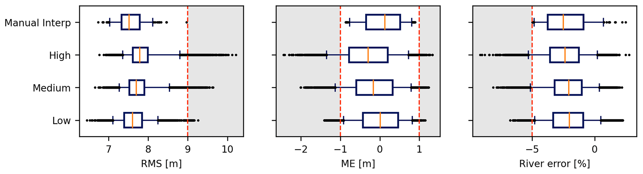
Figure 7Performance in terms of root mean square error (RMS) and mean error (ME) of the hydraulic head and the river error at the discharge station of the realizations within the three uncertainty scenarios (low, medium and high) and the manual interpretation (“Manual Interp”) model. The boxes show the interquartile range between the 25th and 75th percentiles, while the whiskers mark the 5th and 95th percentiles. The median is indicated by the solid orange line. The manual interpretation scenario consists of 200 parameter realizations, while the remaining scenarios each consist of the same 200 parameter realizations combined with 50 hydrostratigraphic realizations.
4.2.2 Predictions
A summary of the uncertainties of the groundwater model predictions is presented in Fig. 8. The mean normalized standard deviation of the median travel time and the mean normalized standard deviation of the capture zone area are shown on the x and y axes, respectively. The mean standard deviation is a measure of the uncertainty within the predictions; it is normalized to the predictions to enable a comparison between them. To obtain the normalized standard deviation, the standard deviation of a parameter or a hydrostratigraphic realization (comprising 50 different hydrostratigraphic realizations or 200 different parameter realizations, respectively) is divided by the ensemble mean prediction. The mean of the normalized standard deviation of the parameter or hydrostratigraphic ensembles is then calculated. Marginal predictions are shown for the hydrostratigraphic realizations (orange) and parameter realizations (blue). Also, the three well fields are shown with different marker types and the three uncertainty scenarios are shown with different marker sizes in Fig. 8.
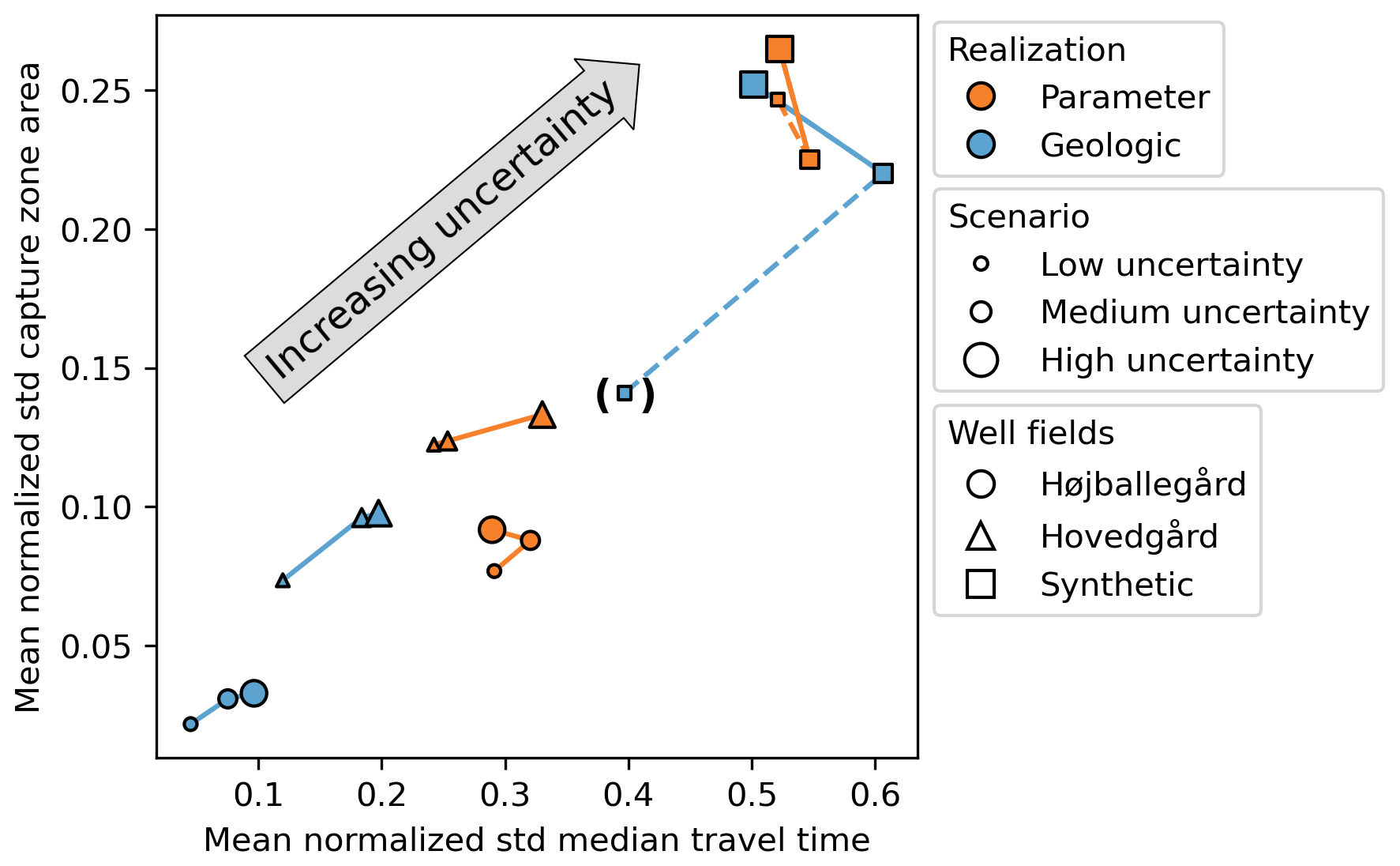
Figure 8Mean normalized standard deviations of the capture zone area and median travel time for all uncertainty scenarios (low, medium and high) and all well fields (Højballegård, Hovedgård and the synthetic well field). The predictions have been marginalized on either parameter realizations (orange) or hydrostratigraphic realizations (blue). For the synthetic well field in the low uncertainty scenario, half of the hydrostratigraphic realizations had to be discarded, and the predictions are therefore placed in parentheses.
At least three effects can be observed in Fig. 8. First, upon comparing the parameter and hydrostratigraphic realizations (different marker colors), the parameter uncertainty is seen to introduce a higher mean normalized standard deviation than the hydrostratigraphic interpretation uncertainty. This is except for the synthetic well field, where the uncertainties introduced into the predictions from the parameters and from the hydrostratigraphy become comparable. Second, when comparing the results across well fields (different marker types), we see that the mean normalized standard deviation of Højballegård well field is lower than that of Hovedgård well field, which is again lower than that of the synthetic well field. Also, upon comparing the results within the different uncertainty scenarios, we see that the scenarios with higher uncertainty generally introduce a higher mean normalized standard deviation for the predictions. Third, when comparing the results for the synthetic well field (square markers) to those for the other two well fields (circle and triangle markers), the difference in the results of the hydrostratigraphic realizations between the uncertainty scenarios is larger in the synthetic well field. Further, the travel time variance does not increase from the medium to the high uncertainty scenario, which is the case for the other two well fields. In the following, these three observations will be elaborated.
4.2.3 Hydrostratigraphic vs. parameter realizations
To illustrate the influence of the hydrostratigraphic realizations on the capture zones, the capture zones in the Højballegård and synthetic well fields for randomly selected realizations are presented in Figs. 9 and 10, respectively. The capture zone areas are shown as probability maps where a value of 100 % signifies that particles placed in that cell are captured by the extraction well for all selected realizations. For each parameter realization (Figs. 9b–e and 10b–e), the results are based on 50 hydrostratigraphic realizations. For each hydrostratigraphic realization (Figs. 9g–j and 10g–j), the results are based on 200 parameter realizations. The capture zone areas for the manual interpretation model (Figs. 9f and 10f) and for all realizations (Figs. 9a and 10a) are also shown for reference.
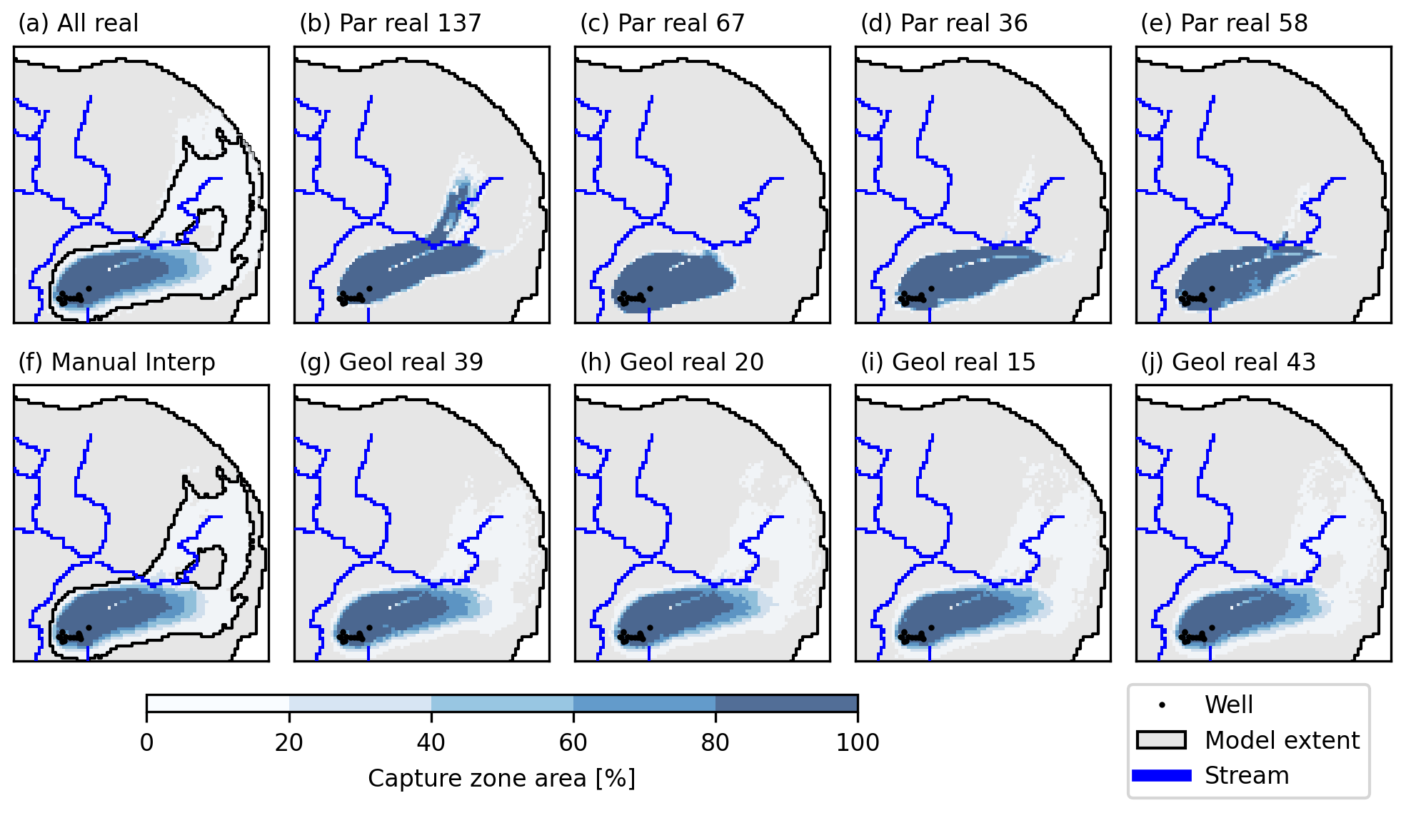
Figure 9The capture zone area of the Højballegård well field in the low uncertainty scenario, as shown on maps of the percentage of realizations. The location of the plot is seen in Fig. 1. Four parameter realizations (“Par real”, b–e) and hydrostratigraphic realizations (“Geol real”, g–j) were randomly selected. In the hydrostratigraphic realizations as well as the manual interpretation model (f), the ensemble consists of 200 parameter realizations, while the ensemble consists of 50 hydrostratigraphic realizations in the parameter realizations. In the “all real” scenario, the ensemble consists of 50 hydrostratigraphic realizations and 200 parameter realizations.
The results for Højballegård shown in Fig. 9 represent the low uncertainty scenario. The simulated capture zone areas for the parameter realizations are dominated by high probability values, implying that the responses from the hydrostratigraphic realizations are similar. Correspondingly, the capture zone areas of the four hydrostratigraphic realizations are similar in extent and shape. On the other hand, the extents covered by the four parameter realizations are more diverse, illustrating a higher degree of disagreement between the parameter realizations. This is also seen for the four hydrostratigraphic realizations, where large parts of the capture zone area are dominated by low probabilities. The capture zone area of the synthetic well field in the high uncertainty scenario (Fig. 10) is at the other end of the spectrum – large parts of the capture zone area have low probabilities in both the hydrostratigraphic and parameter realizations. Correspondingly, the extent of the selected realizations covers different areas for hydrostratigraphic and parameter realizations, indicating that both have a noticeable impact on the extent of the capture zone area.
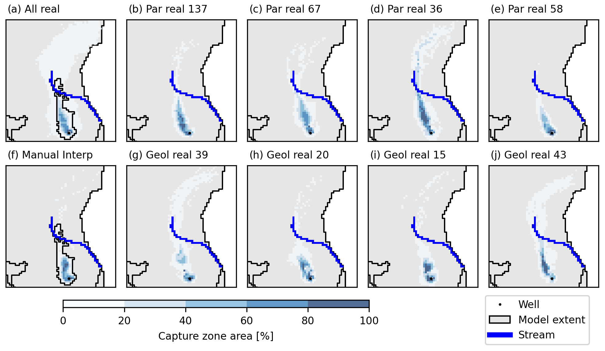
Figure 10The capture zone area of the synthetic well field in the high uncertainty scenario, as shown on maps of the percentage of realizations. The location of the plot is seen in Fig. 1. Four parameter realizations (“Par real”, b–e) and hydrostratigraphic realizations (“Geol real”, g–j) were randomly selected. In the hydrostratigraphic realizations as well as the manual interpretation model (f), the ensemble consists of 200 parameter realizations, while the ensemble consists of 50 hydrostratigraphic realizations in the parameter realizations. In the “all real” scenario, the ensemble consists of 50 hydrostratigraphic realizations and 200 parameter realizations.
4.2.4 Well fields
All capture zone areas in the high uncertainty scenario are illustrated in Fig. 11. The results for the individual parameter realizations are shown in the columns of the matrices while the hydrostratigraphic realizations are shown in the rows. In the legend, two endmembers of the expected variation when the parameter uncertainty dominates and when the hydrostratigraphic uncertainty dominates are shown. Red realization numbers correspond to the randomly selected realizations in Fig. 10. The selected realization of Fig. 9 is not marked here, as it was selected in the low uncertainty scenario. For the Højballegård well field, the matrix has dominant vertical structure, suggesting that the uncertainty is dominated by parameter uncertainty. In contrast, for the synthetic well field, the hydrostratigraphic realizations exert a stronger influence on the capture zone area, with no visually dominant row or column directions. The results for Hovedgård well field are in between those for the other two well fields.
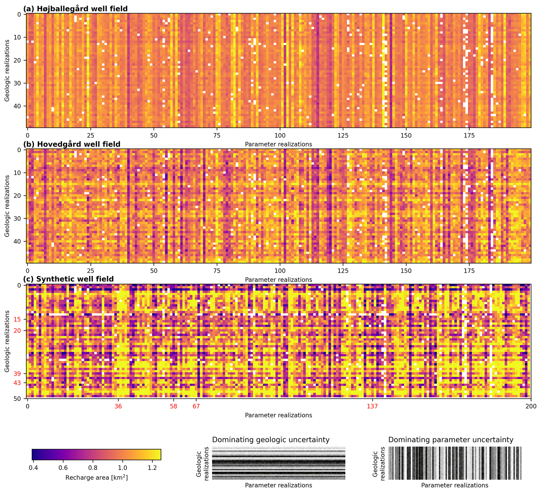
Figure 11Simulated capture zone areas in Højballegård well field, Hovedgård well field and the synthetic well field, as shown in plots of the parameter realizations (columns) versus the hydrostratigraphic realizations (rows) in the high uncertainty scenario.
Figure 2 illustrates the density of each interpretation point category in each well field. At Højballegård, there is a high density of high-certainty (category 1) interpretation points around the well field. The density of interpretation points is lower in Hovedgård and lower still in the synthetic well field. However, as is also evident in Fig. 2, the hydrostratigraphies of the three well fields are different; i.e., Højballegård well field is characterized by large aquifers, while Hovedgård and the synthetic well field have thinner aquifers. Therefore, we cannot isolate the effect that contributes to the highest impact of interpretation uncertainty for the synthetic well field and the lowest impact for Højballegård. We can only conclude that both the hydrostratigraphic structure and the certainty with which it has been described impacts the interpretation uncertainty.
4.2.5 Synthetic well field
Figure 6d–f illustrates the impacts of the uncertainty scenarios on the hydrostratigraphic models, with the yellow layer marking the Miocene sand from where the synthetic well is pumping. In the low uncertainty scenario (Fig. 6d), the Miocene layer has a relatively high elevation compared to the manual interpretation model (Fig. 6e) and other uncertainty scenarios. This is explained by a lack of interpretation points in the area to constrain the hydrostratigraphic model realizations. In half of the realizations, the elevation of the Miocene layer is above the water table (not shown), which means that predictions based on particle tracking cannot be calculated. The impact of the hydrostratigraphic realizations on the predictions in the low uncertainty scenario is therefore underestimated. This explains the large difference in results between the uncertainty scenarios in the synthetic well field (Fig. 8).
Also, in Fig. 6 it can be observed that a red Quaternary sand layer appears in the medium uncertainty scenario and becomes even more prominent in the high uncertainty scenario. Because of the relatively few interpretation points in this area (Fig. 2), the stratigraphy changes between the uncertainty scenarios as the smoothing factor is changed. This may explain why the mean normalized standard deviation does not react the same way in response to the uncertainty scenarios in the synthetic well field as it does in the two real well fields (Fig. 8).
This study demonstrates a methodology to quickly and systematically characterize the interpretation uncertainty of a manual interpretation model and to propagate the characterized interpretation uncertainty to a groundwater model. In the following, the results of the hydrostratigraphic and groundwater modeling will be discussed and will be translated into practical lessons.
5.1 Assessment of the hydrostratigraphic model
Expectations of the relative impact of the interpretation uncertainty were met by the results; i.e., the interpretation uncertainty in areas of high certainty in the hydrostratigraphic model (Højballegård well field) was shown to have a relatively small impact on predictions, while the impact was more pronounced in areas with less geological certainty (synthetic well field). The results showed that scenarios with higher geological uncertainty generate higher variation of predictions. The results support the expected applicability of the method for incorporating geological interpretation uncertainty in groundwater models.
Nevertheless, the results from the synthetic well field were not as expected. The synthetic well field was shown to give rise to the largest predictive variance. As opposed to the real well fields, borehole information from the well does not inform the geology in this well field. The modeled uncertainty in this area is therefore higher than what would be expected in most real-case well fields. It was shown that the layer sequence in the synthetic well field area is different from that in the original manual interpretation model in the hydrostratigraphic realizations (Fig. 6), while the layer sequence does not differ in the other well fields. Thus, the characterized uncertainty within the hydrostratigraphic realizations in the synthetic well field had a different character from that in the other well fields. To limit the risk of changes to the stratigraphy in areas with a low density of interpretation points, the applied methodology could be extended as follows: (1) an expert knowledge filter could be applied to the resulting hydrostratigraphic realizations to ensure that the realizations comply with a set of stratigraphic rules in specific areas or (2) nonstationarity could be introduced such that the expected small-scale variability in the model can vary across the study area. This would likely add more uncertainty in areas of high interpretation uncertainty, thus making synthetic wells behave more predictably.
5.2 Assessment of the groundwater model
The predictions from the groundwater models were calculated with a suite of parameters, which allowed the original interpretation model to replicate the measured system behavior. To obtain the suite of parameters, the GLUE approach was applied, which is an informal Bayesian approach. According to Vrugt et al. (2009), the parameter uncertainty from a GLUE approach is larger than that from a formal Bayesian approach. The parameter uncertainty may therefore be inflated compared to what it would have been if a formal Bayesian approach had been applied. However, only a few parameters were involved in the analysis of the parameter uncertainty. The inclusion of more parameters in the uncertainty analysis would likely lead to an increase in estimated parameter uncertainty.
When applying the parameters from the original manual interpretation model, the replication of system behavior was shown to deteriorate slightly as more interpretation uncertainty was introduced into the uncertainty scenarios (Fig. 7). This in turn gave rise to an increase in predictive variance between geological uncertainty scenarios (Fig. 8). Thus, some inaccuracies must be anticipated if we assume that the posterior parameter range from the interpretation model is applicable to other hydrostratigraphic realizations. However, this assumption was deemed necessary to make the problem computationally tractable, as the alternative is to perform a calibration of all hydrostratigraphic realizations. Another alternative is simulation-based learning to obtain the posterior distribution for the different scenarios (Hermans et al., 2023; Thibaut et al., 2021).
As only one out of many possible parameter uncertainty estimation methods were applied, and considering the uniqueness of the study area in terms of geology and data density, no general conclusions will be drawn here about the relative importance of geological interpretation uncertainty and parameter uncertainty. However, in this study, a limited influence of the interpretation uncertainty compared to the parameter uncertainty for predictions of capture zone area and median travel time was found in a geologically well-defined area with thick aquifers. In a geologically poorly defined area with thin aquifers, the influence of interpretation uncertainty and the influence of parameter uncertainty became comparable. Other studies testing the uncertainty of the hydrostratigraphic model have concluded that the model structure is dominant compared to the parameter uncertainty (e.g., Højberg and Refsgaard, 2005). The difference is that, in this study, only the interpretation uncertainty within a given conceptual model was characterized, not the conceptual uncertainty itself. Given that the presented level of uncertainty is a fair representation, our results thereby confirm existing evidence (e.g., Neuman and Wierenga, 2003; Rojas et al., 2010) that the choice of the conceptual model has a far greater impact on the groundwater model predictions than the interpretation uncertainty within the manually interpreted model.
5.3 Lessons of a practical nature
This study's generalizability is restricted by the specific characteristics of the study area. Egebjerg is geologically very complex, with several generations of buried valleys crossing each other, glaciotectonic disturbed layers, and a deep fault zone disturbing the layers. So, even though the area is relatively data dense and a well-defined conceptual model has been developed, the hydrostratigraphic connections between the layers are uncertain due to the geological complexity of the area. It has therefore been questioned whether the area can be accurately represented by a simple layer model (Enemark et al., 2022). This geological complexity of the area also results in relatively poor performance of the groundwater model, with the best root mean square error being around 7 m, indicating potential flaws in the conceptual understanding.
For practical purposes, at least in Denmark, a buffer zone is often added to the capture zone area simulated by a groundwater model based on a single hydrostratigraphic model to take account of unspecified uncertainty (Iversen et al., 2009). Two problems relate to the application of the buffer-zone approach: (1) the necessary width of the buffer zone is determined based on a subjective assessment of the uncertainty in the area, and (2) a simple buffer zone cannot capture spatial trends in the capture zone area that do not expand radially. From a management point of view, this is not ideal, as areas that are not part of the real capture zone may be included, while other relevant areas may be excluded. However, in the case where the impact of the interpretation uncertainty is low (Fig. 9a), the buffer approach with, e.g., a 200 m buffer around the manual interpretation model from Fig. 9f appears to be sufficient to capture the uncertainty in the capture zone area. The approach presented in this study offers an alternative to the buffer-zone approach at the expense of an increase in computational time but with the benefit of higher certainty that a more realistic capture zone area has been obtained.
From an interpretation point of view, our results indicate limited differences between the low, medium and high uncertainty scenario. This suggests that the geological interpreter can feel more at ease during interpretation as to whether the exact location of the layer boundary has been identified correctly. The impact of interpretation uncertainty within a conceptual model is highly dependent on the geological structures and complexity, implying that precise interpretations are needed more in areas with thin aquifers (such as the area around the synthetic well field) than in areas with thick and laterally extensive aquifers (such as around Højballegård well field). The scale of the influence is also dependent on the data density and quality for the area. As the Egebjerg study area is a data-dense area, future work should include areas with data availabilities that are closer to the average or even low, where the influence of interpretation uncertainty will likely be higher.
While the interpretation uncertainty of a deterministic hydrostratigraphic model is a known accessory, it has until recently been difficult to propagate these uncertainties from the hydrostratigraphic model to a groundwater model. This study has shown an approach to systematically characterize the impact of hydrostratigraphic model interpretation uncertainties in groundwater modeling. The applied groundwater model was a full 3D model in which the vertical discretization follows the hydrostratigraphic units. Results showed that it is possible to represent the interpretation uncertainty in areas with low geological uncertainty containing thick, large aquifers with a buffer zone; however, in areas of high geological uncertainty with thinner, smaller aquifers, the interpretation uncertainty could be just as significant as the parameter uncertainty. This study confirms that if the uncertainty of the conceptual model is small, the small-scale variability within the conceptual model is of less importance. This suggests that, in a geological modeling exercise, it is more worthwhile to invest time in developing a clearly defined conceptual model or even better multiple conceptual models. The actual interpretation of data using the conceptual model(s) is of less importance for the groundwater model predictions.
The hydrostratigraphical realization generation code is currently not publicly accessible in a repository, as it has been developed within research projects that lack funding for code documentation. If you wish to obtain the code, please reach out to Rasmus Bødker Madsen at rbm@geus.dk, and it will be provided upon request.
The data/models for generating the hydrostratigraphical realizations are available at https://doi.org/10.22008/FK2/EA0OET (Madsen, 2023).
The supplement related to this article is available online at: https://doi.org/10.5194/hess-28-505-2024-supplement.
RBM oversaw the modeling of different scenarios of geological uncertainty. TE performed groundwater modeling and the subsequent analysis. ASH initiated the original idea. PBES, LTA, IM and ASH provided valuable insights into geological uncertainties and interpretations, while TS, KHJ and JK assisted in the analysis of the groundwater data. All authors contributed to the interpretation, analysis and discussion of the results. RBM, ASH and TE prepared the first draft of the manuscript with contributions from all co-authors.
The contact author has declared that none of the authors has any competing interests.
Publisher’s note: Copernicus Publications remains neutral with regard to jurisdictional claims made in the text, published maps, institutional affiliations, or any other geographical representation in this paper. While Copernicus Publications makes every effort to include appropriate place names, the final responsibility lies with the authors.
The quality of this manuscript was improved by the reviews by Thomas Hermans, Mark Bierkens and one anonymous reviewer.
This research has been supported by GeoCenter Danmark under the GeoConcept project and by the Innovation Fund Denmark (grant no. 7017-00160B).
This paper was edited by Harrie-Jan Hendricks Franssen and reviewed by Marc Bierkens, Thomas Hermans, and one anonymous referee.
Andersen, L. T. and Sandersen, P. B. E.: GeoConcept – 3D hydrostratigrafisk lagmodel for Egebjerg (GEUS report 2020/59), 64 pp., https://doi.org/10.22008/gpub/34556, 2020.
Bakker, M., Post, V., Langevin, C. D., Hughes, J. D., White, J. T., Starn, J. J., and Fienen, M. N.: Scripting MODFLOW Model Development Using Python and FloPy, Groundwater, 54, 733–739, https://doi.org/10.1111/gwat.12413, 2016.
Barfod, A. A. S., Vilhelmsen, T. N., Jørgensen, F., Christiansen, A. V., Høyer, A.-S., Straubhaar, J., and Møller, I.: Contributions to uncertainty related to hydrostratigraphic modeling using multiple-point statistics, Hydrol. Earth Syst. Sci., 22, 5485–5508, https://doi.org/10.5194/hess-22-5485-2018, 2018.
Benoit, N., Marcotte, D., and Molson, J.: Stochastic correlated hydraulic conductivity tensor calibration using gradual deformation, J. Hydrol., 594, 125880, https://doi.org/10.1016/j.jhydrol.2020.125880, 2021.
Beven, K. J. and Binley, A.: The future of distributed models: Model calibration and uncertainty prediction, Hydrol. Process., 6, 279–298, https://doi.org/10.1002/hyp.3360060305, 1992.
Christiansen, A. V. and Auken, E.: A global measure for depth of investigation, Geophysics, 77, 4, https://doi.org/10.1190/geo2011-0393.1, 2012.
Curtis, A.: The science of subjectivity, Geology, 40, 95–96, https://doi.org/10.1130/focus012012.1, 2012.
Danielsen, J. E., Auken, E., Jørgensen, F., Søndergaard, V. H., and Sørensen, K. I.: The application of the transient electromagnetic method in hydrogeophysical surveys, J. Appl. Geophys., 53, 181–198, 2003.
Enemark, T., Andersen, L. T., Høyer, A.-S., Jensen, K. H., Kidmose, J., Sandersen, P. B. E., and Sonnenborg, T. O.: The influence of layer and voxel geological modelling strategy on groundwater modelling results, Hydrogeol. J., 30, 617–635, https://doi.org/10.1007/s10040-021-02442-9, 2022.
Feyen, L. and Caers, J.: Quantifying geological uncertainty for flow and transport modeling in multi-modal heterogeneous formations, Adv. Water Resour., 29, 912–929, https://doi.org/10.1016/j.advwatres.2005.08.002, 2006.
GeoScene3D: http://www.geoscene3d.com, last access: 16 March 2023.
Hansen, B., Sonnenborg, T. O., Møller, I., Bernth, J. D., Høyer, A. S., Rasmussen, P., Sandersen, P. B. E., and Jørgensen, F.: Nitrate vulnerability assessment of aquifers, Environ. Earth Sci., 75, 999, https://doi.org/10.1007/s12665-016-5767-2, 2016.
Harrar, W. G., Sonnenborg, T. O., and Henriksen, H. J.: Capture zone, travel time, and solute-transport predictions using inverse modeling and different geological models, Hydrogeol. J., 11, 536–548, https://doi.org/10.1007/s10040-003-0276-2, 2003.
He, X., Sonnenborg, T. O., Jørgensen, F., Høyer, A.-S., Møller, R. R., and Jensen, K. H.: Analyzing the effects of geological and parameter uncertainty on prediction of groundwater head and travel time, Hydrol. Earth Syst. Sci., 17, 3245–3260, https://doi.org/10.5194/hess-17-3245-2013, 2013.
Henriksen, H. J., Troldborg, L., Sonnenborg, T., Højberg, A. L., Stisen, S., Kidmose, J. B., and Refsgaard, J. C.: Hydrologisk geovejledning: God praksis i hydrologisk modellering, GEUS, 130 pp., https://doi.org/10.22008/gpub/38284, 2017 (in Danish).
Hermans, T., Goderniaux, P., Jougnot, D., Fleckenstein, J. H., Brunner, P., Nguyen, F., Linde, N., Huisman, J. A., Bour, O., Lopez Alvis, J., Hoffmann, R., Palacios, A., Cooke, A.-K., Pardo-Álvarez, Á., Blazevic, L., Pouladi, B., Haruzi, P., Fernandez Visentini, A., Nogueira, G. E. H., Tirado-Conde, J., Looms, M. C., Kenshilikova, M., Davy, P., and Le Borgne, T.: Advancing measurements and representations of subsurface heterogeneity and dynamic processes: towards 4D hydrogeology, Hydrol. Earth Syst. Sci., 27, 255–287, https://doi.org/10.5194/hess-27-255-2023, 2023.
Hills, R. G. and Wierenga, P. J.: INTRAVAL Phase II Model Testing at the Las Cruces Trench Site, NUREG/CR-6063, https://www.oecd-nea.org/upload/docs/application/pdf/2019-12/intraval2wg1.pdf (last access: 22 January 2024), 1994.
Højberg, A. L. and Refsgaard, J. C.: Model uncertainty – parameter uncertainty versus conceptual models, Water Sci. Technol., 52, 177–186, 2005.
Høyer, A.-S., Jørgensen, F., Lykke-Andersen, H., and Christiansen, A. V.: Iterative modelling of AEM data based on a priori information from seismic and borehole data, Near Surf. Geophys., 12, 635–650, 2014.
Høyer, A.-S., Jørgensen, F., Sandersen, P. B. E., Viezzoli, A., and Møller, I.: 3D geological modelling of a complex buried-valley network delineated from borehole and AEM data, J. Appl. Geophys., 122, 94–102, https://doi.org/10.1016/j.jappgeo.2015.09.004, 2015.
Høyer, A.-S., Vignoli, G., Hansen, T. M., Vu, L. T., Keefer, D. A., and Jørgensen, F.: Multiple-point statistical simulation for hydrogeological models: 3-D training image development and conditioning strategies, Hydrol. Earth Syst. Sci., 21, 6069–6089, https://doi.org/10.5194/hess-21-6069-2017, 2017.
Høyer, A.-S., Klint, K. E. S., Fiandaca, G., Maurya, P. K., Christiansen, A. V., Balbarini, N., Bjerg, P. L., Hansen, T. B., and Møller, I.: Development of a high-resolution 3D geological model for landfill leachate risk assessment, Eng. Geol., 249, 45–59, https://doi.org/10.1016/j.enggeo.2018.12.015, 2019.
Høyer, A.-S., Sandersen, P. B. E., Andersen, L. T., Madsen, R. B., Mortensen, M. H., and Møller, I.: Uncertainty Assessments in 3D Geological Modelling of Complex Unconsolidated Sediments – with Emphasis on Handling Subjectivity in the Entire Workflow, https://doi.org/10.2139/ssrn.4444386, 2023.
Huysmans, M. and Dassargues, A.: Application of multiple-point geostatistics on modelling groundwater flow and transport in a cross-bedded aquifer (Belgium), Hydrogeol. J., 17, 1901–1911, https://doi.org/10.1007/s10040-009-0495-2, 2009.
Iversen, C. H., Lauritsen, L. U., Nyholm, T., and Kürstein, J.: Geo-Vejledning 2: Udpegning af indvindings- og grundvandsdannende oplande (Del 1) – Vejledning i oplandsberegninger i forbindelse med den nationale grundvandskortlægning, GEUS Special Publication, Copenhagen, Denmark, 1–105 pp., https://doi.org/10.22008/gpub/43084, 2009 (in Danish).
Jørgensen, F., Møller, R. R., Sandersen, P. B. E., and Nebel, L.: 3-D Geological Modelling of the Egebjerg Area, Denmark, Based on Hydrogeophysical Data, Geol. Surv. Den. Greenl., 20, 27–30, https://doi.org/10.34194/geusb.v20.4892, 2010.
Jørgensen, F., Møller, R. R., Nebel, L., Jensen, N. P., Christiansen, A. V., and Sandersen, P. B. E.: A method for cognitive 3D geological voxel modelling of AEM data, B. Eng. Geol. Environ., 72, 421–432, https://doi.org/10.1007/s10064-013-0487-2, 2013.
Journel, A. and Zhang, T.: The necessity of a multiple-point prior model, Math. Geol., 38, 591–610, https://doi.org/10.1007/s11004-006-9031-2, 2006.
Li, Z., Wang, X., Wang, H., and Liang, R. Y.: Quantifying stratigraphic uncertainties by stochastic simulation techniques based on Markov random field, Eng. Geol., 201, 106–122, 2016.
Madsen, R. B., Kim, H., Kallesøe, A. J., Sandersen, P. B. E., Vilhelmsen, T. N., Hansen, T. M., Christiansen, A. V., Møller, I., and Hansen, B.: 3D multiple-point geostatistical simulation of joint subsurface redox and geological architectures, Hydrol. Earth Syst. Sci., 25, 2759–2787, https://doi.org/10.5194/hess-25-2759-2021, 2021.
Madsen, R. B., Høyer, A. S., Andersen, L. T., Møller, I., and Hansen, T. M.: Geology-driven modeling: A new probabilistic approach for incorporating uncertain geological interpretations in 3D geological modeling, Eng. Geol., 309, 106833, https://doi.org/10.1016/j.enggeo.2022.106833, 2022.
Madsen, R. B.: Replication Data for: “Incorporating interpretation uncertainties from deterministic 3D hydrostratigraphic models in groundwater models” – (https://doi.org/10.5194/hess-2023-74)), Dataverse [data set] https://doi.org/10.22008/FK2/EA0OET, 2023.
Mariethoz, G. and Caers, J.: Multiple-point geostatistics: Stochastic modeling with training images, 1st edn., John Wiley & Sons, 360 pp., https://doi.org/10.1002/9781118662953, 2015.
Moore, C. and Doherty, J.: Role of the calibration process in reducing model predictive error, Water Resour. Res., 41, 1–14, https://doi.org/10.1029/2004WR003501, 2005.
Neuman, S. P. and Wierenga, P. J.: A Comprehensive Strategy of Hydrogeologic Modeling and Uncertainty Analysis for Nuclear Facilities and Sites, NUREG/CR-6805, 311 pp., https://www.nrc.gov/docs/ML0324/ML032470827.pdf (last access: 22 January 2024), 2003.
Niswonger, R. G., Panday, S., and Motomu, I.: MODFLOW-NWT, A Newton Formulation for MODFLOW-2005, U.S. Geological Survey Techniques and Methods 6-A37, MODFLOW-NWT, 44 pp. https://doi.org/10.3133/tm6A37, 2011.
Poeter, E. and Anderson, D.: Multimodel ranking and inference in ground water modeling, Ground Water, 43, 597–605, https://doi.org/10.1111/j.1745-6584.2005.0061.x, 2005.
Pollock, D. W.: User Guide for MODPATH Version 6 – A Particle-Tracking Model for MODFLOW: U.S. Geological Survey Techniques and Methods 6-A41, 58 pp., https://doi.org/10.3133/tm6A41, 2012.
Refsgaard, J. C., van der Sluijs, J. P., Brown, J., and van der Keur, P.: A framework for dealing with uncertainty due to model structure error, Adv. Water Resour., 29, 1586–1597, https://doi.org/10.1016/j.advwatres.2005.11.013, 2006.
Refsgaard, J. C., Christensen, S., Sonnenborg, T. O., Seifert, D., Højberg, A. L., and Troldborg, L.: Review of strategies for handling geological uncertainty in groundwater flow and transport modeling, Adv. Water Resour., 36, 36–50, https://doi.org/10.1016/j.advwatres.2011.04.006, 2012.
Rojas, R., Batelaan, O., Feyen, L., and Dassargues, A.: Assessment of conceptual model uncertainty for the regional aquifer Pampa del Tamarugal – North Chile, Hydrol. Earth Syst. Sci., 14, 171–192, https://doi.org/10.5194/hess-14-171-2010, 2010.
Royse, K. R.: Combining numerical and cognitive 3D modelling approaches in order to determine the structure of the Chalk in the London Basin, Comput. Geosci., 36, 500–511, https://doi.org/10.1016/j.cageo.2009.10.001, 2010.
Sandersen, P. B. E.: Uncertainty assessment of geological models – A qualitative approach, IAHS-AISH Publ., 345–349, 2008.
Sandersen, P. B. E. and Jørgensen, F.: Kortlægning af begravede dale i Danmark (Mapping of Buried Valleys in Denmark), Opdatering 2015 (Update 2015), Vol. 1 and 2, GEUS Special Publication, Copenhagen, Denmark, ISBN 978-87-7871-451-0, 2016 (in Danish).
Sandersen, P. B. E., Jørgensen, F., Kallesøe, A. J., and Møller, I.: Geo-vejledning 2018/1 – Opstilling af geologiske modeller til grundvandsmodellering, GEUS Special Publication, Copenhagen, Denmark, 1–224 pp., https://doi.org/10.22008/gpub/38283, 2018 (in Danish).
Seifert, D., Sonnenborg, T. O., Refsgaard, J. C., Højberg, A. L., and Troldborg, L.: Assessment of hydrological model predictive ability given multiple conceptual geological models, Water Resour. Res., 48, 1–16, https://doi.org/10.1029/2011WR011149, 2012.
Stafleu, J., Maljers, D., Gunnink, J. L., Menkovic, A., and Busschers, F. S.: 3D modelling of the shallow subsurface of Zeeland, the Netherlands, Geol. en Mijnbouw/Netherlands J. Geosci., 90, 293–310, https://doi.org/10.1017/S0016774600000597, 2011.
Thibaut, R., Laloy, E., and Hermans, T.: A new framework for experimental design using Bayesian Evidential Learning: The case of wellhead protection area, J. Hydrol., 603, 126903, https://doi.org/10.1016/j.jhydrol.2021.126903, 2021.
Troldborg, L., Refsgaard, J. C., Jensen, K. H., and Engesgaard, P.: The importance of alternative conceptual models for simulation of concentrations in a multi-aquifer system, Hydrogeol. J., 15, 843–860, https://doi.org/10.1007/s10040-007-0192-y, 2007.
Troldborg, L., Ondracek, M., Koch, J., Kidmose, J., and Refsgaard, J. C.: Quantifying stratigraphic uncertainty in groundwater modelling for infrastructure design, Hydrogeol. J., 29, 1075–1089, https://doi.org/10.1007/s10040-021-02303-5, 2021.
Viezzoli, A., Jørgensen, F., and Sørensen, C.: Flawed Processing of Airborne EM Data Affecting Hydrogeological Interpretation, Groundwater, 51, 191–202, https://doi.org/10.1111/j.1745-6584.2012.00958.x, 2013.
Vignoli, G., Fiandaca, G., Christiansen, A. V., Kirkegaard, C., and Auken, E.: Sharp spatially constrained inversion with applications to transient electromagnetic data, Geophys. Prospect., 63, 243–255, 2015.
Vrugt, J. A., ter Braak, C. J. F., Gupta, H. V., and Robinson, B. A.: Equifinality of formal (DREAM) and informal (GLUE) Bayesian approaches in hydrologic modeling?, Stoch. Environ. Res. Risk Assess., 23, 1011–1026, https://doi.org/10.1007/s00477-008-0274-y, 2009.
Wellmann, F. and Caumon, G.: 3-D Structural Geological Models: Concepts, Methods, and Uncertainties, Adv. Geophys., 59, 1–121, https://doi.org/10.1016/bs.agph.2018.09.001, 2018.
Zhang, J. Z., Huang, H. W., Zhang, D. M., Phoon, K. K., Liu, Z. Q., and Tang, C.: Quantitative evaluation of geological uncertainty and its influence on tunnel structural performance using improved coupled Markov chain, Acta Geotech., 16, 3709–3724, 2021.