Assessing rainfall radar errors with an inverse stochastic modelling framework

Weather radar is a crucial tool for rainfall observation and forecasting, providing high-resolution estimates in both space and time. Despite this, radar rainfall estimates are subject to many error sources – including attenuation, ground clutter, beam blockage and drop-size distribution – with the true rainfall field unknown. A flexible stochastic model for simulating errors relating to the radar rainfall estimation process is implemented, inverting standard weather radar processing methods and imposing path-integrated attenuation effects, a stochastic drop-size-distribution field, and sampling and random errors. This can provide realistic weather radar images, of which we know the true rainfall field and the corrected “best-guess” rainfall field which would be obtained if they were observed in a real-world case. The structure of these errors is then investigated, with a focus on the frequency and behaviour of “rainfall shadows”. Half of the simulated weather radar images have at least 3 % of their significant rainfall rates shadowed, and 25 % have at least 45 km² containing rainfall shadows, resulting in underestimation of the potential impacts of flooding. A model framework for investigating the behaviour of errors relating to the radar rainfall estimation process is demonstrated, with the flexible and efficient tool performing well in generating realistic weather radar images visually for a large range of event types.

1 Introduction

Precipitation is challenging to measure accurately, due to its intermittent nature, spatio-temporal variability and sensitivity to environmental conditions (Savina et al., 2012). For urban hydrology, weather radar plays an increasingly important role in quantitative precipitation estimation, due to the high spatio-temporal resolution of the information needed (Thorndahl et al., 2017). The small sizes of urban catchments and the intended hydrological applications – particularly for real time or near real time – require information about precipitation fields at small temporal and spatial scales, from 1–10 min and 1–5 km, respectively (Berne et al., 2004; Ochoa-Rodriguez et al., 2015; De Vos et al., 2017; Thorndahl et al., 2017; Shehu and Haberlandt, 2021).

Despite the suitability of weather radar for obtaining high-resolution rainfall estimates, there are many sources of error in the estimation process, with different sources of uncertainty reviewed in numerous studies (Michelson et al., 2005; Meischner, 2005; Villarini and Krajewski, 2010; Ośróka et al., 2014; Ciach and Gebremichael, 2020). Errors include radar calibration and stability problems, contamination by clutter and anomalous propagation, occultation, a beam-broadening effect with non-uniform beam filling, attenuation and assumptions made about the drop-size distribution (DSD) (Marshall and Palmer, 1948; Harrison et al., 2000). Some error sources can be corrected for, such as bias and systematic errors, ground clutter (Gabella and Notarpietro, 2002; Ventura and Tabary, 2013; Li et al., 2013) and attenuation (Nicol and Austin, 2003; Krämer, 2008; Jacobi and Heistermann, 2016), resulting in significantly improved reliability. Correction procedures are often limited due to the cumulative nature of errors from a superposition of different sources, with complex approaches showing only modest improvements to estimates. Information on the rainfall field is lost, irretrievable, and we do not even know how often this happens.

There is therefore an ongoing need to account for errors in the radar rainfall estimation process (Villarini and Krajewski, 2010; Seo et al., 2018), and uncertainties should be acknowledged and modelled (Ciach et al., 2007; Gires et al., 2012; Villarini et al., 2014; Rico-Ramirez et al., 2015). The poor quantification of uncertainties was highlighted as a fundamental issue in AghaKouchak et al. (2010a) and expanded in AghaKouchak et al. (2010b). An error model described in Hasan et al. (2014) found that uncertainties were easily identifiable for unbiased reflectivity–rainfall (Z–R) relationships, incorporating radar reflectivity uncertainties in Hasan et al. (2016). Variograms were used to represent radar rainfall uncertainties (Cecinati et al., 2017), eliminating the need for a covariance matrix for faster and more flexible calculation of the spatial correlation of errors. Uijlenhoet and Berne (2008) created a stochastic model of range profiles for the DSD, using a Monte Carlo framework (Berne and Uijlenhoet, 2006) to estimate uncertainties using two attenuation correction schemes. Yan et al. (2021) imposed random and non-linear radar errors on simulated rainfall fields, with Z–R relationship errors appearing to have little influence overall.

Error quantification is challenging, and errors propagate into future estimates for any model which requires rainfall as an input. The fundamental limitation in radar correction is that the “true” rainfall field is not available for comparisons. In this study, the aim is to work backwards to obtain an estimate of the uncertainty in the radar rainfall estimation process. Using a new model for simulating realistic space–time rainfall event fields with high resolution (matching that of a UK standard C-band weather radar) (Green et al., 2024), a clustered parameterization based on radar rainfall events from High Moorsley weather radar operated by the UK Met Office was extracted. These simulation outputs are treated as the true rainfall field. Errors relating to each step of the radar rainfall estimation process are then imposed on the simulated rainfall field to obtain an ensemble of spatio-temporal error fields for each event in a stochastic manner, forming a superposition of different error sources. This is done by inverting standard radar processing methods, allowing identification of the frequency of the occurrence and extent of the loss of important information.

In this study, the data and study area are first discussed in Sect. 2, together with the simulation methods applied to obtain realistic space–time rainfall fields. The methodology for the radar error model is then outlined in detail in Sect. 3, with detailed explanations for each step of the model. Example event results are discussed in Sect. 4.2–4.5, with more general results based on event images given in Sect. 4.6–4.9. A discussion and conclusions are given in Sect. 5, with model limitations, potential for generalization and future work also discussed.

2 Data

An ensemble of realistic rainfall events is used, generated using the clustered rainfall model outlined in Green et al. (2024). This model uses fast Fourier transform (FFT) methods to efficiently generate three-dimensional rainfall event fields with a high resolution matching that of radar data (1 km, 5 min) for a 200×200 km domain. Events have prescribed properties, including the correlation structure, spatial anisotropy, spatio-temporal anisotropy, marginal distribution, non-zero rainfall proportions and advection. The model is used with multi-dimensional scaling and hierarchical clustering to parameterize rainfall event simulations for 100 rainfall events.

A year of processed dual-polarization C-band weather radar data is used to parameterize simulations of realistic space–time rainfall fields. This is obtained from weather radar from High Moorsley (Met Office, 2003), which is located near Durham, England (54°48^′20^′′ N, 001°28^′32^′′ W), with a wavelength and frequency of 5.3 cm and 5.6 GHz, respectively. This operates between five elevation angles from 0.5 to 2° with 1° beam width, taking a scan at each elevation approximately every 5 min.

3 Radar error model

This section outlines a novel model for imposing errors in the radar rainfall estimation process on a rainfall field, focusing on four main error sources: random noise effects, attenuation effects, DSD error and sampling through estimation variance. Section 3.1–3.3 describe the error model in more detail, outlined in Fig. 1 and written in Python. While the model is by no means comprehensive, random error is included. This is designed to provide a framework for investigating the impact of these errors, improving understanding of the estimation process.

Figure 1 Schematic for imposing the radar error model on simulated rainfall fields, outlined in more detail in Sect. 3.1–3.5.

3.1 Re-projecting to polar coordinates

The simulated rainfall fields are given on a regular three-dimensional Cartesian grid. To apply radar processing methods in reverse, the data must be re-projected into a polar coordinate system. Using nearest-neighbour interpolation methods, the Cartesian grid is converted into polar data

$$\begin{array}{}\text{(1)}& Z(t,x,y)\to Z(t,\mathit{\theta },r)\end{array}$$

for ray angles $\mathit{\theta }=\mathrm{1},\mathrm{2},\mathrm{\dots }\mathrm{360}$ with ray bins $r=\mathrm{1},\mathrm{2},\mathrm{\dots }\mathrm{167}$ of width 600 m and average elevation angle 1°. This mirrors the radar configuration of the High Moorsley weather radar used for parameterization. The different elevation angles and the differences in the sampling sizes of the pixels are incorporated through the use of estimation variance in Sect. 3.5.

3.2 Attenuation effects

A constrained gate-by-gate approach is applied to estimate the path-integrated attenuation (PIA) for each radar ray by inverting standard forward-attenuation models (Krämer and Verworn, 2008; Jacobi and Heistermann, 2016). Inverting the process gives an estimated attenuated reflectivity Z_i rate for the ith bin of width Δr as

$$\begin{array}{}\text{(2)}& \begin{array}{rl}& \widehat{Z_i}=Z_{i,\mathrm{corr}}-\sum _{j=\mathrm{0}}^{i-\mathrm{1}}\widehat{k_j}\text{ and}\\ & \widehat{k_i}=c{\left[Z_{\mathrm{corr},i}+(\mathrm{2}\mathrm{\Delta }r-\mathrm{1})\sum _{j=\mathrm{0}}^{i-\mathrm{1}}\widehat{k_j}\right]}^d\end{array}\end{array}$$

for constants c and d. This results in a realistic radar image of attenuated reflectivity in a polar coordinate system at each time step of the event, denoted by $Z_{\mathrm{corr}}(t,\mathit{\theta },r)$. Using the scheme described above, for rainfall intensity R(t) at time t, we get a PIA estimate PIA(t) of

$$\begin{array}{}\text{(3)}& \stackrel{\mathrm{̃}}{R}\left(t\right)=\left\{\begin{array}{ll}R\left(t\right)-{\mathrm{PIA}}_{\mathrm{R}\left(t\right)}\left(t\right)& \mathrm{if}R\left(t\right)\ge {\mathrm{PIA}}_{\mathrm{R}\left(t\right)}\left(t\right),\\ \mathrm{0}& \mathrm{otherwise},\end{array}\right.\end{array}$$

where PIA(t)=f{R(t)} is a function based on the estimation algorithm outlined in Jacobi and Heistermann (2016).

3.3 Random noise effects

When considering empirical variograms for weather radar images, Pegram and Clothier (2001) found that 10 % of the variability in images corresponded to nugget effects, highlighting the need for random noise effects in radar pixel simulations. This noise is also evident in the marginal distributions of radar images, with the full year and an example “dry” day image for the High Moorsley weather radar given in Fig. 2, showing a large number of values in the range −32 to 0 dBZ. Although rainfall rates of less than 0.01 mm h⁻¹ are hardly noticeable in terms of rainfall accumulations, this high density of low-reflectivity rates in radar images may have a significant effect on attenuation estimates along the radar rays. This noise may be attributed to the measuring apparatus, non-meteorological echoes or most likely a combination of various different sources. Errors are treated as random noise, representing a combination of errors from unknown sources clearly evident in real radar images.

Figure 2 Histograms of an example dry radar image (blue) and all radar pixels above −32 dBZ (orange) for the High Moorsley weather radar for the year 2019, where u_nz is the reflectivity rate corresponding to the non-zero rainfall threshold of 0.1 mm h⁻¹.

The random noise field is added to rainfall values to prevent numerical instabilities, with the marginal distribution from Fig. 2 converted to rainfall rates in Fig. 3. When considering the logarithm of weather radar noise (i.e. dry day images and values (dBZ) corresponding to rainfall rates less than 0.1 mm h⁻¹), these are sufficiently Gaussian to satisfy the assumption of a log-normal marginal distribution for random noise effects. A log-normal marginal distribution allows for a simple and easy transformation when simulating the field using Gaussian random field theory. Empirical variograms of these values were estimated to identify an appropriate correlation structure, which has a very short correlation range of around 5 km. The optimal spatial transformation for minimizing least squares between the marginal variogram values of the two spatial dimensions is used to estimate field anisotropy from empirical variogram fields, with estimates suggesting that isotropy of random noise fields is a valid assumption in this case. The three-dimensional noise field denoted by $\mathit{\epsilon }(t,x,y)$ is assumed to be log-normal, with a marginal distribution of

$$\begin{array}{}\text{(4)}& \mathit{\epsilon }\sim \mathrm{LN}\left({\mathit{\mu }}_{\mathit{\epsilon }},{\mathrm{\Sigma }}_{\mathit{\epsilon }}^{\mathrm{2}}\right),\end{array}$$

where ${\mathit{\mu }}_{\mathit{\epsilon }}=-\mathrm{5.3}$ and σ_ε=1.7. A Gaussian random field is simulated with an exponential correlation structure of ${\mathit{\rho }}_{\mathit{\epsilon }}\left(h\right)=\exp \mathit{\{}-h/r_{\mathit{\epsilon }}\mathit{\}}$ for a short range with r_ε=5 and a nugget effect of n_ε=0.35. This is transformed using an inverse Gaussian score transformation and then exponentiated, resulting in a random noise field with the desired marginal distribution and correlation structure. An example field is included in Fig. 3, from which we can see that the variability is slightly higher than in existing images. This is however selected to preserve the proportion of −32 dBZ reflectivity rates in images, with any values less than −32 dBZ treated as −32 dBZ.

Figure 3 Histograms of low rainfall rates (and logarithms) corresponding to empirical random noise (i.e. in the range $-\mathrm{32}<Z\le \mathrm{10}$) obtained from High Moorsley weather radar for the year 2019 (blue), together with an example simulated noise field (orange).

3.4 Drop-size-distribution errors

Attenuated rainfall rates $\stackrel{\mathrm{̃}}{R}\left(t\right)$ can then be added to the three-dimensional noise field $\mathit{\epsilon }(t,x,y)$, which can then be converted into a reflectivity field. A Z–R relationship is typically used, of the form Z=10log ₁₀(aR^b) for reflectivity Z (dBZ), rainfall R (mm h⁻¹) and constants a and b, which typically take the values a=200 and b=1.6 (Harrison et al., 2000). Constant values for a and b are based on the assumption that the DSD varies spatially and temporally in a way characteristic of a particular rainfall or weather type. Despite this, a fixed Z–R relationship results in a severe underestimation of peak rainfall intensities due to the failure to account for natural variations in the DSD with intensity (Schleiss et al., 2020). Lee et al. (2007) indicated that the overall DSD variability cannot be adequately explained by a single parameter. In Libertino et al. (2015), a varying Z–R relationship in space and time improved rainfall accumulations at the event scale when compared to a fixed relationship.

A large amount of scatter around the average power-law relationship is related to the various microphysical processes that are responsible for the DSD variability. To account for this variability, in an attempt to generate more realistic reflectivity images, we assume that $a=A(x,y)$ is a two-dimensional field varying in space. As the simulated rainfall events all have a fairly short duration (6 h or less), a constant DSD in time is initially used. This assumes that A is fairly constant over the time period considered, although the model is flexible and the dimensions of A can easily be extended to include time.

Parameters in the Z–R relationship typically take values in the ranges $a\in (\mathrm{30},\mathrm{1000})$ and $b\in (\mathrm{0.8},\mathrm{2})$ (Battan and Theiss, 1973; Smith and Krajewski, 1993), and so parameter b is still treated as constant but is sampled from a Gaussian distribution with a low variance centred around a value of μ_b=1.6. This gives attenuated reflectivity estimates of

$$\begin{array}{}\text{(5)}& \stackrel{\mathrm{̃}}{Z}\left(t\right)=\mathrm{10}{\log }_{\mathrm{10}}\left\{A{\left[\stackrel{\mathrm{̃}}{R}\left(t\right)+\mathit{\epsilon }\left(t\right)\right]}^b\right\}\end{array}$$

for

$$\begin{array}{}\text{(6)}& A(x,y)\sim N_{\mathrm{2}}\left({\mathit{\mu }}_a,\mathit{\{}\mathrm{1}+g(x,y\left)\mathit{\right\}}{\mathrm{\Sigma }}_a\right)b\sim N\left({\mathit{\mu }}_b,{\mathit{\sigma }}_b^{\mathrm{2}}\right)\end{array}$$

for correlation structure ${\mathit{\rho }}_a={\mathit{\sigma }}_a\exp \mathit{\{}-h/r_a\mathit{\}}$, where μ_a=220, σ_a=2, r_a=30, μ_b=1.6 and σ_b=0.02. The function $g(x,y)={\mathrm{\Sigma }}_E(x,y)$ is the estimation variance based on the pixel location (x, y) and on the proportion of the rainfall volume that the radar can see for a given distance, which is discussed further in Sect. 3.5. Attenuated reflectivity fields are rounded to one decimal place and are limited by a minimum value of −32 dBZ, as is the case for actual reflectivity data.

3.5 Radar sampling

Due to the nature of weather radar sampling, polar observations close to the receiver sample from a much smaller volume than those further away, as can be seen for an example pixel in Fig. 4. Earth curvature effects, cloud height and bright band effects also impact the sampling volume, and furthermore radar observations above the freezing level are unavailable due to the high reflectivity of melting precipitation (Hooper and Kippax, 1950; Kitchen et al., 1994; Hall et al., 2015).

Figure 4 Schematic of a radar ray sampling volume for an example pixel, denoted as a vertical column.

To address this, sampling errors are included as part of the DSD model designed to increase uncertainty in the DSD where the volume of rainfall sampled by the radar beam is lower. Areas where it is unrealistic for the radar beam to be sampling rainfall (e.g. above the bright band level or outside the base and top of the cloud) are removed with flexible model parameters which can be adjusted. In this case, the configuration of High Moorsley weather radar is used (see Sect. 2).

The radar sampling error is defined using estimation variance principles by representing the change in uncertainty between the actual and sampled volumes. Assuming a pixel is a vertical column denoted by V dependent on the radar configuration and the distance of the pixel from the weather radar, parts of this vertical column will be sampled by the radar, denoted by ν (see Fig. 6). The estimation variance σ_E can be defined as

$$\begin{array}{}\text{(7)}& {\mathit{\sigma }}_{\mathrm{E}}=\mathrm{2}\stackrel{\mathrm{‾}}{\mathit{\gamma }}(V,\mathit{\nu })-\stackrel{\mathrm{‾}}{\mathit{\gamma }}(\mathit{\nu },\mathit{\nu })-\stackrel{\mathrm{‾}}{\mathit{\gamma }}(V,V),\end{array}$$

where $\stackrel{\mathrm{‾}}{\mathit{\gamma }}$ is the mean variogram and V and ν are the total and sampled volumes, respectively. By discretizing the vertical pixel into small blocks, we can estimate the empirical variograms in Eq. (7), with an example of discretized blocks contributing to each term in Fig. 5 based on a variogram model for the vertical distribution of the DSD.

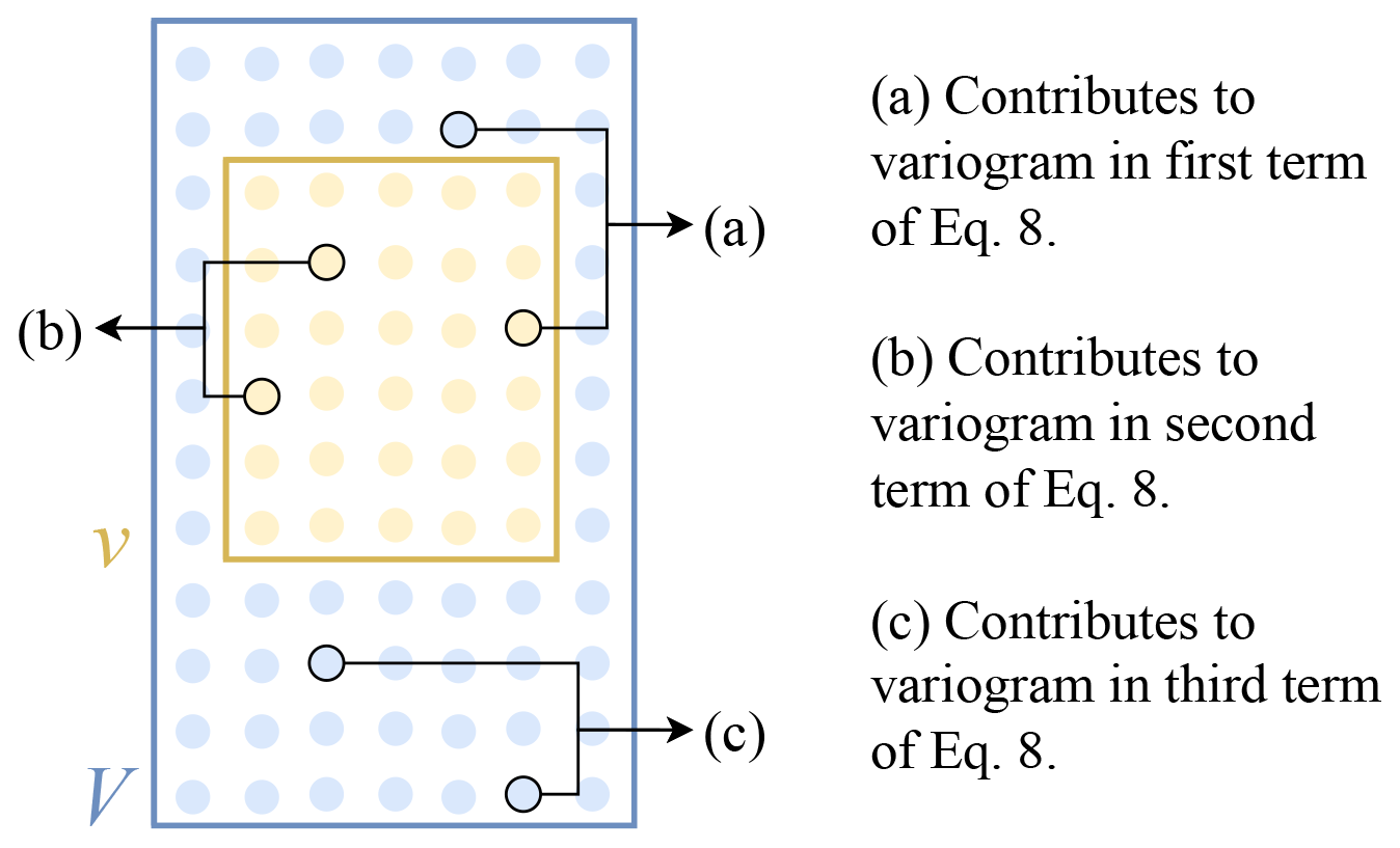
Figure 5 Example of variogram contributions for a discretized volume V. A given volume ν is sampled, highlighting an example of discretized blocks contributing to empirical variogram estimation for each of the terms in Eq. (7).

We consider a vertical column of rainfall, assuming that the cloud base, bright band and cloud top are 1, 4 and 10 km and assuming an exponential variogram model for below the bright band level. Discretizing the vertical column of rainfall into blocks of height 10 m (see Fig. 6), the empirical distances for each discretized block are calculated using the variogram model. Parameterization is based on analyses of vertical weather radar data (Berne et al., 2005), considering the vertical raindrop volume distribution for a range of rainfall rates and heights. The variance of sampling volumes in different ranges supported the concept, with simulations compared to vertical radar images for validation.

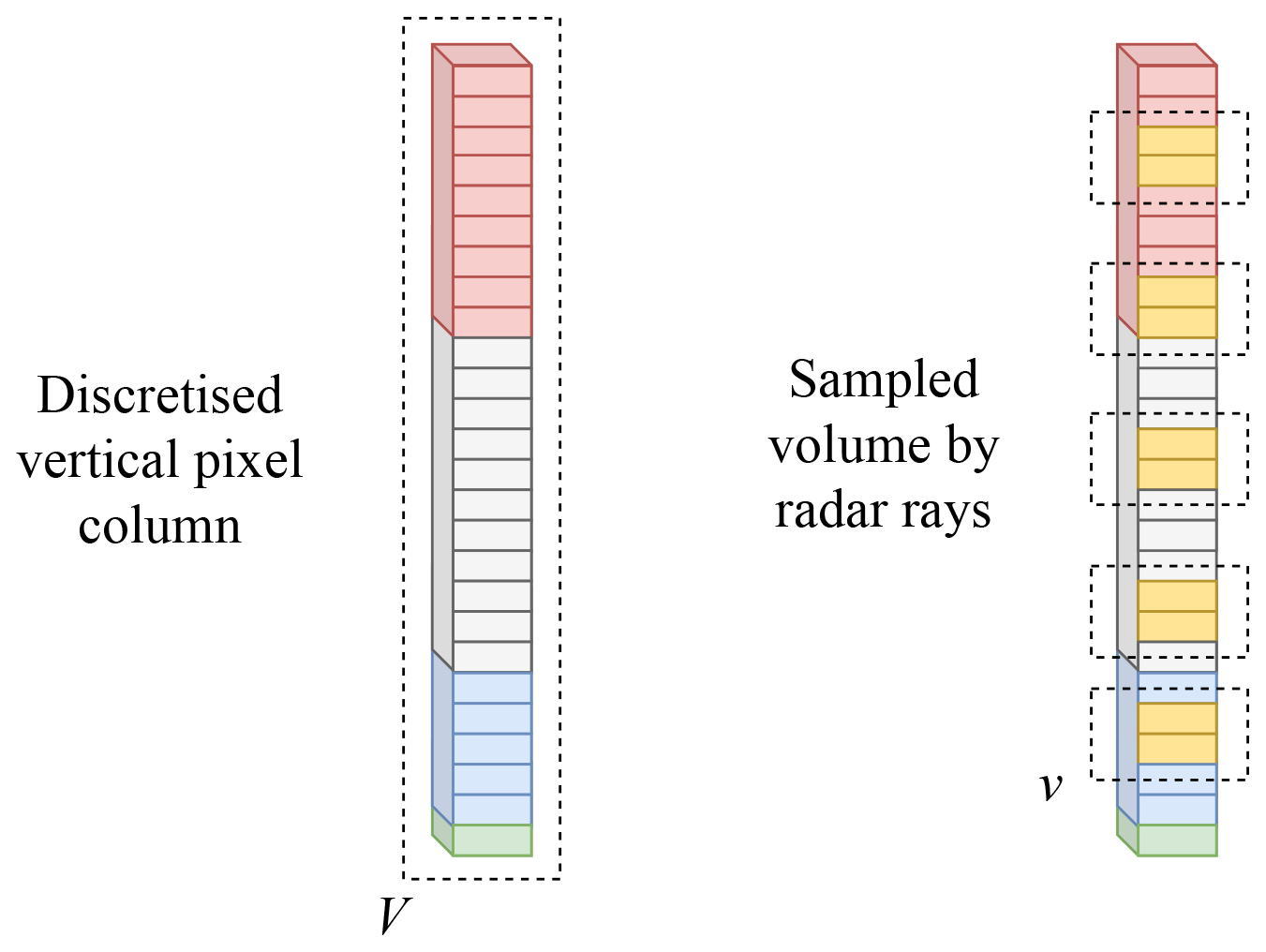
Figure 6 Example of the vertical structure of a rainfall pixel, with discretized blocks representing the volume V and the volume sampled by the radar beam ν highlighted in yellow.

4 Results

In this section, the performance of the model is considered by looking at example fields for each step of the simulation process. We consider 100 rainfall events simulated using the methods outlined in Green et al. (2024) and parameterized by radar rainfall events from High Moorsley weather radar (see Sect. 2). For each event, the model was run n=100 times to obtain an ensemble of weather radar images. To enable direct comparisons, each radar image is corrected using a standard radar rainfall estimation process resulting in corrected rainfall for each ensemble member, similar to what would be obtained from a radar rainfall image. This includes an attenuation correction (Jacobi and Heistermann, 2016), a Z–R relationship (Harrison et al., 2017) and re-projection onto a Cartesian grid to allow for direct comparisons with the original simulated rainfall field R.

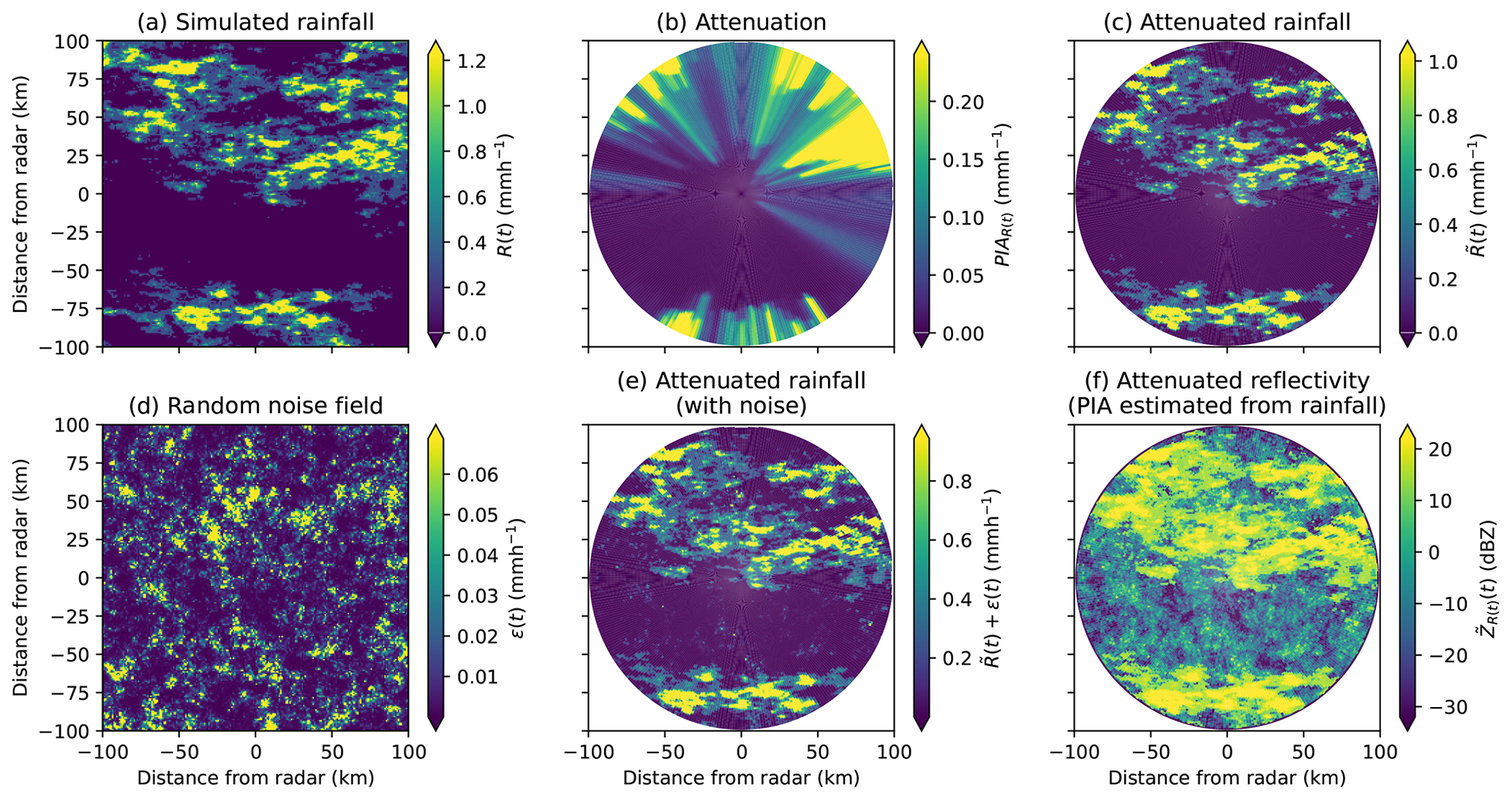
Figure 7 Step-by-step error model fields, including the (a) simulated rainfall field R(t), (b) attenuation PIA, (c) attenuated rainfall $\stackrel{\mathrm{̃}}{R}\left(t\right)$, (d) random noise field ε(t), (e) attenuated rainfall with random noise $\stackrel{\mathrm{̃}}{R}\left(t\right)+\mathit{\epsilon }\left(t\right)$ and (f) attenuated reflectivity $\stackrel{\mathrm{̃}}{Z}\left(t\right)$ for a single time step of an example simulated event.

Defining the difference between the simulated true rainfall field (R) and the corrected rainfall field (R_corr,i) after applying the radar error model as the error, we consider specific events R, individual event time steps R(t) throughout the ensemble (i.e. image-based) and the behaviour of all events. To investigate the capacity of the radar error model to capture uncertainty, we consider the error metrics outlined below.

1. The mean bias between corrected ensemble members and original simulated rainfall

   $$\begin{array}{}\text{(8)}& \mathrm{BIAS}\left(R\right)={\displaystyle \frac{\mathrm{1}}{n}}\sum _{i=\mathrm{1}}^n\left(R-R_{\mathrm{corr},i}\right)\end{array}$$

   for ensemble members i=1, …, 100

2. The root-mean-square error (RMSE) across the ensemble

   $$\begin{array}{}\text{(9)}& \mathrm{RMSE}\left(R\right)=\sqrt{{\displaystyle \frac{\mathrm{1}}{n}}\sum _{i=\mathrm{1}}^n{\left(R-R_{\mathrm{corr},i}\right)}^{\mathrm{2}}}\end{array}$$

3. The pixel variability throughout the ensemble, using the standard deviation

   $$\begin{array}{}\text{(10)}& \mathrm{SD}\left(R_{\mathrm{corr}}\right)=\sqrt{{\displaystyle \frac{\sum _{i=\mathrm{1}}^n{\left(R_{\mathrm{corr},i}-{\stackrel{\mathrm{‾}}{R}}_{\mathrm{corr},i}\right)}^{\mathrm{2}}}{n}}}\end{array}$$

4. The minimum and maximum RMSE values across the ensemble

   $$\begin{array}{}\text{(11)}& \begin{array}{rl}& {\mathrm{RMSE}}_{\min }\left(R\right)={\min }_{i=\mathrm{1},\mathrm{\dots },n}\left\{\sqrt{{\left(R-R_{\mathrm{corr},i}\right)}^{\mathrm{2}}}\right\}\text{and}\\ & {\mathrm{RMSE}}_{\max }\left(R\right)={\max }_{i=\mathrm{1},\mathrm{\dots },n}\left\{\sqrt{{\left(R-R_{\mathrm{corr},i}\right)}^{\mathrm{2}}}\right\}\end{array}\end{array}$$

5. The average error across the ensemble, as a percentage of the original simulated rainfall field for all non-zero simulated rainfall pixels

   $$\begin{array}{}\text{(12)}& p_{\mathrm{R}}={\displaystyle \frac{\mathrm{1}}{n}}\sum _{i=\mathrm{1}}^n\left(\mathrm{1}-{\displaystyle \frac{R_{\mathrm{corr},i}}{R}}\right)\times \mathrm{100}\mathit{\%}\end{array}$$

   where R>0.

Additional metrics are defined to identify cases where significant amounts of rainfall are missing in corrected rainfall fields. Crane (1979) referred to distortions in storm structures, as a result of attenuation, as shadows. In this study we define rainfall shadows as areas where information about the rainfall field is lost from a simulated weather radar image after correction methods have been applied. A formal definition of a rainfall shadow in this case is taken to be a pixel where the simulated rainfall is significant (i.e. R>1 mm h⁻¹) but the corrected rainfall is much lower (less than 10 %) than the original simulated rate (i.e. $R_{\mathrm{corr}}/R\le \mathrm{0.1}|R>\mathrm{1}$).

We first consider example fields for each stage of the error model in Sect. 4.1 and then three events which show high bias and low and high variability in Sect. 4.2–4.4, quantified based on the above metrics at an event level. The behaviour of individual radar images is considered by looking at the average, minimum and maximum behaviours over the ensemble, including the variability. Attempts are made to find metrics and properties of rainfall images with the aim of identifying instances where there is a very high level of uncertainty or error arising from the rainfall estimation process. The impact of the rainfall location with respect to the radar is considered, together with identifying how often significant information on the rainfall field is lost. For individual image-based errors, we introduce three image metrics below relating to rainfall shadows:

1. ARS is the actual area (km²) of the radar image that contains rainfall shadows.

2. LARS is the largest single area (km²) of rainfall shadows in a radar image.

3. PRS is the proportion of significant rainfall (i.e. R>1 mm h⁻¹) that is shadowed.

Figure 8 (a) Simulated rainfall field, (b) example reflectivity and (c) corrected rainfall field for simulated event A (video link at https://zenodo.org/record/8029394/files/true_sim_rainfall_133.mp4?download=1, last access: 16 October 2024).

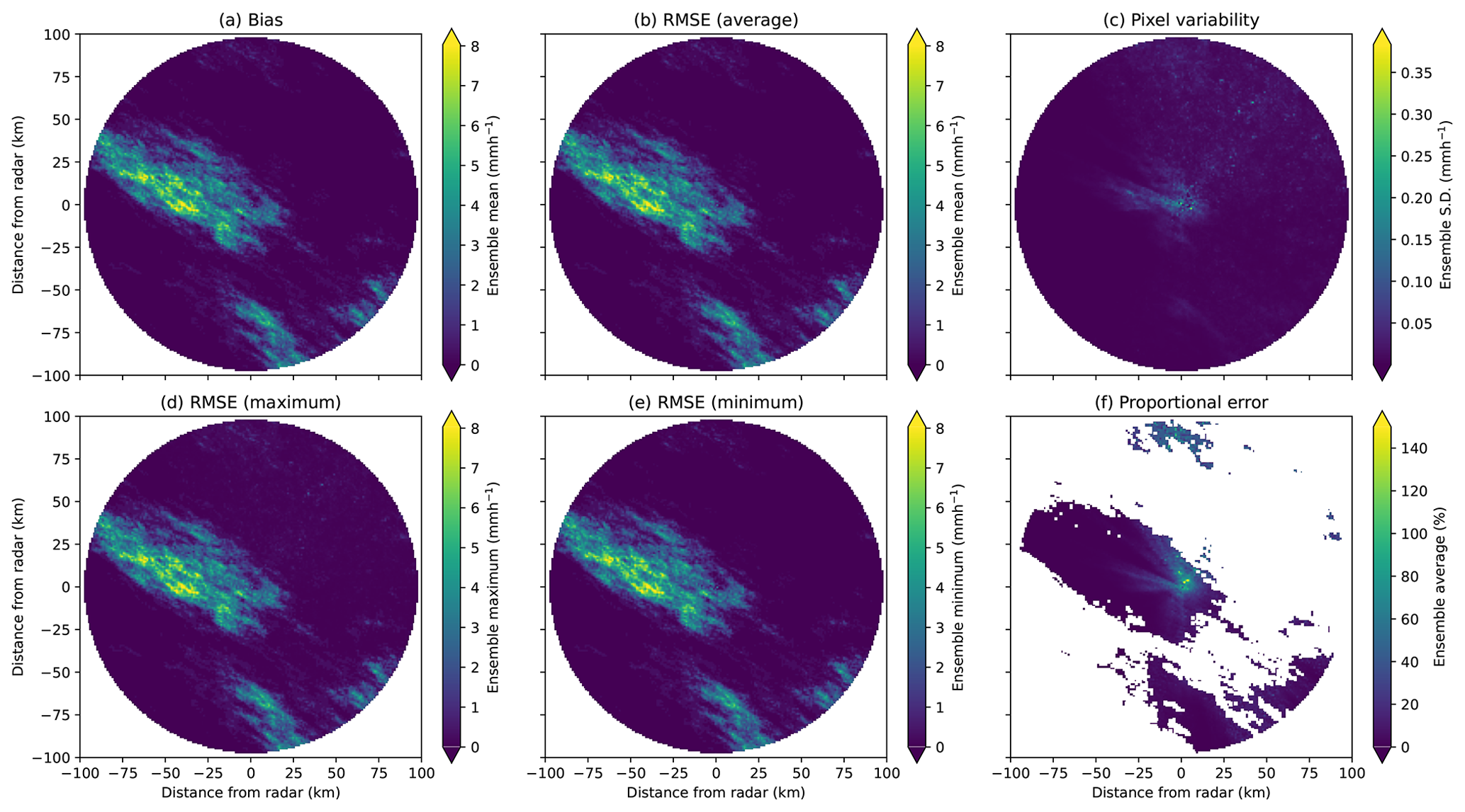
Figure 9 (a) Average bias, (b) average RMSE, (c) pixel variability (SD), (d) maximum RMSE, (e) minimum RMSE and (f) average proportional error for simulated event A (video link at https://zenodo.org/record/8029394/files/errors_and_var133.mp4?download=1, last access: 16 October 2024).

4.1 Example fields

For an example time step of a simulated event, each stage of the radar error model process is given in Fig. 7. The final radar image (Fig. 7f) appears realistic, with clear areas of rainfall similar to raw radar images obtained from the High Moorsley weather radar. A significant proportion of the signal is attenuated towards the edge of the domain, particularly in the top right of the image.

4.2 Event A: high bias

The event shown in Fig. 8a has an area of moderate-intensity rainfall in the centre of the image with a large extent, resulting in high bias. The simulated radar image for an ensemble member associated with the event looks realistic, with the reflectivity and corrected rainfall rates (see Fig. 8b and c) showing significant rainfall amounts missing throughout. The average bias, RMSE and pixel variability corresponding to the event in Fig. 8 are given in Fig. 9. The average bias and RMSE are very high (see Fig. 9a and b), taking values over 5 mm h⁻¹.

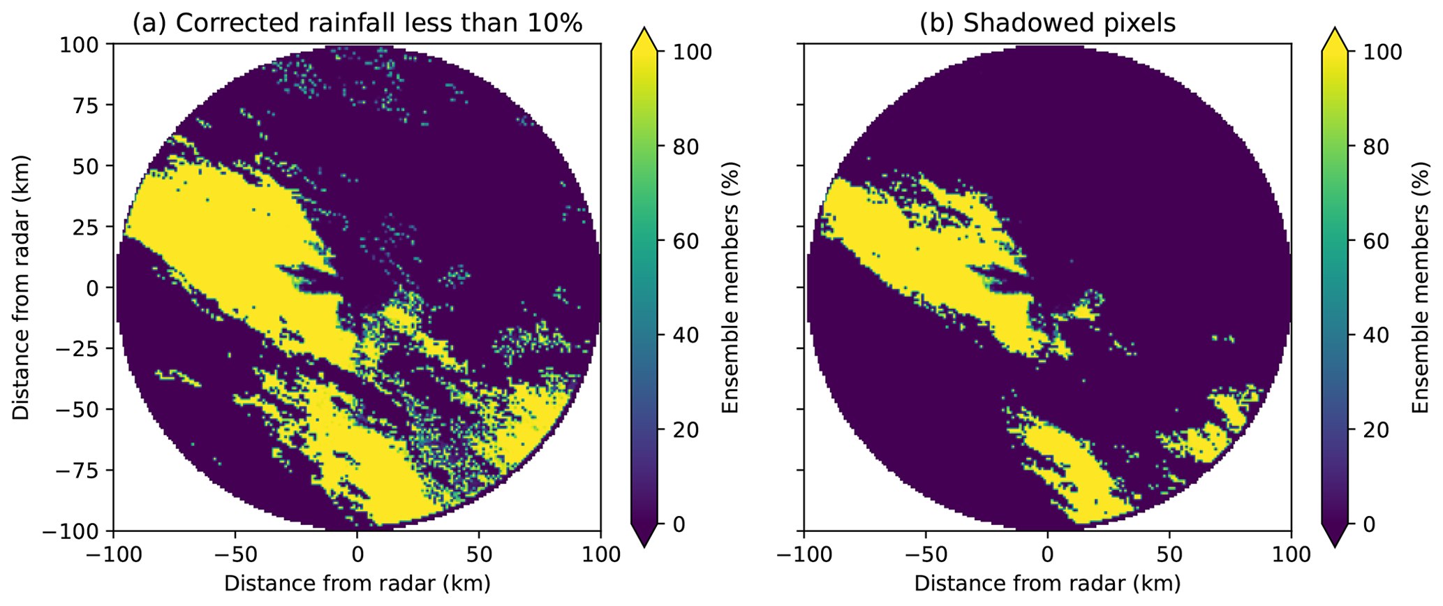
Figure 10 (a) Percentage of corrected rainfall that is less than 10 % of the original simulated field and (b) frequency of shadowed pixels over the ensemble for simulated event A (video link at https://zenodo.org/record/8029394/files/shadowed_133.mp4?download=1, last access: 16 October 2024).

Figure 11 (a) Simulated rainfall field, (b) example reflectivity and (c) corrected rainfall field for simulated event B (video link at , last access: 16 October 2024).

Figure 9c shows very low pixel variability for most of the image, which is reflected in the range of RMSE values throughout the ensemble given in Fig. 9d and e, with a large area in the centre of the image showing a bias and RMSE greater than 5 mm h⁻¹, suggesting that the rainfall is consistently underestimated throughout the ensemble. A large area of moderate-intensity rainfall on top of the radar is overcorrected, mimicking effects resulting from full attenuation of the radar signal by intervening rainfall. In this case, the correction techniques will not improve the image significantly, and so information on a large portion of the rainfall field is lost, particularly when forward-attenuation correction algorithms are implemented.

This result is reiterated when looking at the rainfall shadows in Fig. 10b, where around one-fourth of the image is shadowed for 100 % of the ensemble members. This event has a very high average bias, with pixel variability varying drastically throughout the image. Large areas of rainfall are missing, and the differing variability throughout and spatial distribution of the error structure suggest that a mean field bias or multiplicative correction would not improve the estimates significantly. The information on the rainfall structure and rates would be lost in this case.

4.3 Event B: low variability

Figure 11a shows a rainfall event with a small extent of light rainfall and mostly dry conditions throughout the image, resulting in low variability throughout the simulated ensemble. There is a small amount of light rainfall in the centre left of the radar domain, with the corrected rainfall image in Fig. 11c exhibiting lower rainfall rates here than the original simulated rainfall. The radar image in Fig. 11 appears realistic, with a small amount of signal damping towards the left of the image in a range beyond the rainfall seen in Fig. 11a.

Figure 12 (a) Average bias, (b) average RMSE, (c) pixel variability (SD), (d) maximum RMSE, (e) minimum RMSE and (f) average proportional error for simulated event B (video link at https://zenodo.org/record/8029394/files/errors_and_var49.mp4?download=1, last access: 16 October 2024).

Figure 13 (a) Percentage of corrected rainfall that is less than 10 % of the original simulated field and (b) frequency of shadowed pixels over the ensemble for simulated event B (video link at https://zenodo.org/record/8029394/files/shadowed_49.mp4?download=1, last access: 16 October 2024).

The corresponding bias and RMSE for this event are given in Fig. 12, together with the pixel variability and maximum and minimum RMSEs over the ensemble and the average proportional error. Over the ensemble, the average bias (see Fig. 12a) is close to zero, except for the low-intensity rainfall areas (with at most 0.5 mm h⁻¹), with low average, minimum and maximum RMSEs in Fig. 12b, d and e. The pixel variability is slightly higher in the rainfall area (see Fig. 12c), with pixels at a larger distance from the transmitter in this area showing lower pixel variability (less than 0.02 mm h⁻¹) and the remaining variability appearing uniform. In Fig. 13b, the rainfall is shadowed in 100 % of the rainfall ensemble (i.e. all the ensemble members) in the area of low-intensity rainfall identified in Fig. 11. The frequency of shadows over the ensemble mostly has values of either zero or one. This event has very low variability between the ensemble members, likely due to (mostly) non-zero rainfall amounts in the images.

Figure 14 (a) Simulated rainfall field, (b) example reflectivity and (c) corrected rainfall field for simulated event C, with high-intensity rainfall (average throughout the event over 10 mm h⁻¹) highlighted in red (video link at https://zenodo.org/record/8029394/files/true_sim_rainfall_64.mp4?download=1, last access: 16 October 2024).

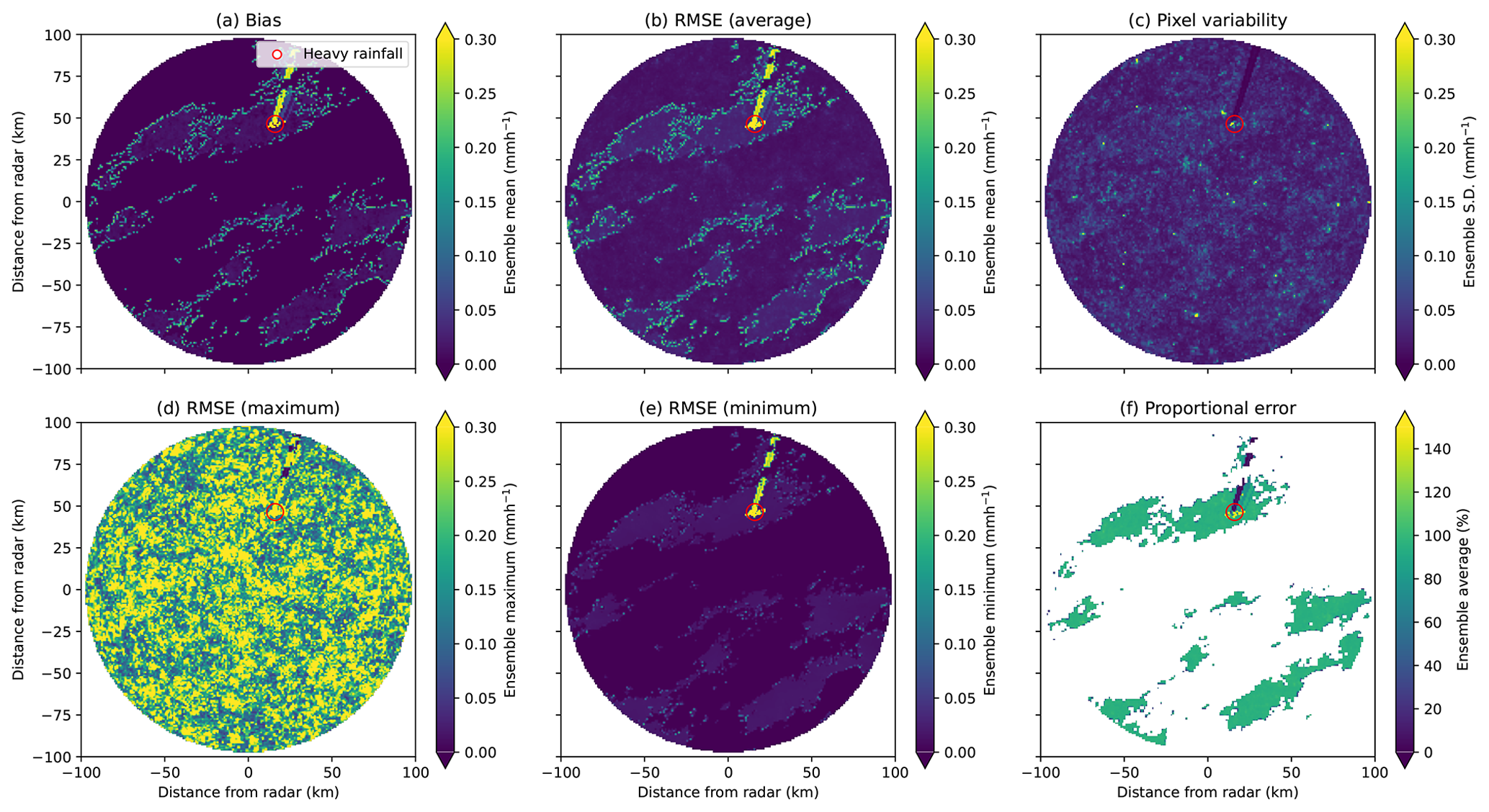
Figure 15 (a) Average bias, (b) average RMSE, (c) pixel variability (SD), (d) maximum RMSE, (e) minimum RMSE and (f) average proportional error for simulated event C, with high-intensity rainfall (average throughout the event over 10 mm h⁻¹) highlighted in red (video link at https://zenodo.org/record/8029394/files/errors_and_var64.mp4?download=1, last access: 16 October 2024).

4.4 Event C: high variability

Figure 14 shows an event with a small area of heavy rainfall rates, which results in high variability in event errors. Most of the radar domain shows zero rainfall rates, except for a very small area of high-intensity rainfall (greater than 100 mm h⁻¹) towards the top of the domain. The example radar image (see Fig. 14b) is again realistic, showing mostly noise. Radial lines in the top right past a small amount of high-intensity rainfall suggest that attenuation effects have not been sufficiently corrected. In Fig. 14c the corrected rainfall image has areas of high-intensity rainfall which are overestimated due to cumulative errors introduced as part of forward-attenuation correction procedures. Although there is no large area of high-intensity rainfall, the rainfall field's spatial distribution has still been significantly impacted by the errors caused by attenuation.

From Fig. 15a and b, these radial lines show a positive average. However, none of these exceeds 0.2 mm h⁻¹. Errors are not noticeable from the maximum RMSE field but have a much higher minimum RMSE than the rest of the image (see Fig. 15d and e). In this case, it appears that the attenuated high-intensity rainfall has been overcorrected, showing an average proportional error greater than one. Pixels within the affected rays at distances further from the radar transmitter are underestimated. Although these are mostly light rainfall rates, the rays have been significantly impacted, showing a clear gap when comparing the simulated and corrected rainfall fields.

Figure 16 (a) Percentage of corrected rainfall less than 10 % of the original simulated field and (b) frequency of shadowed pixels over the ensemble for simulated event C, with high-intensity rainfall (average throughout the event over 10 mm h⁻¹) highlighted in red (video link at https://zenodo.org/record/8029394/files/shadowed_64.mp4?download=1, last access: 16 October 2024).

The shadowed pixels in Fig. 16 show radial lines in areas where the corrected rainfall is less than 10 % of the simulated rainfall. Most of these pixels do not have significant rainfall rates and so are not classed as shadowed, with only a handful of pixels showing shadows and none for 100 % of the ensemble, resulting in high variability within the ensemble.

From the videos of event errors, this high-intensity rainfall moves across the image, affecting different rays, with some pixels showing rainfall shadows past the high-intensity rainfall. This is not consistent throughout the ensemble, with most pixels showing shadows in less than 100 % of the ensemble members. This small area of high-intensity rainfall has resulted in high variability across the ensemble, which is impacted significantly by the overestimation of high-intensity rainfall rates, with the DSD error also contributing to the variability for such a high rainfall rate.

4.5 Specific events: summary

In cases where the absolute bias is low, rainfall shadows may still exist, suggesting that average bias is a poor metric to use when identifying event errors. Even with a low absolute bias, the rainfall could be overestimated for pixels closer to the radar and underestimated past these pixels (which is very common along radar rays where attenuation has been overestimated). In these cases, the spatial distribution of rainfall is often incorrect, which could have detrimental effects when using the rainfall fields for any quantitative modelling. Typically, events with high bias correspond to events with large rainfall shadows, with shadow frequencies close to either zero or one, suggesting that, in cases where there is high bias, the model uncertainty is low. Simulated rainfall events which exhibited high ensemble variability resulted from potential interactions between small areas of high-intensity rainfall and DSD errors, which corresponded to higher variability in shadows throughout the ensemble. Videos of all the simulated events (and the corresponding errors) are available in Green (2023).

4.6 Individual image-based errors: average ensemble behaviour

The relationship between the average rainfall rate and the proportion of rainfall in an image with the image RMSE is shown in Fig. 17a, showing that events with high average rainfall rates and large, heavy rainfall proportions have the highest RMSE. Images showing fairly low proportions (i.e. 5 %–10 %) of heavy rainfall still exhibit a fairly high RMSE. Figure 17b shows the relationship between the mean and standard deviation of non-zero rainfall rates with the image RMSE, showing a higher RMSE for events with a high average and standard deviation in non-zero rainfall rates. This may be due to the large errors resulting in large gradients between pixels, where a large rainfall rate along a ray damps the signal so that subsequent observations are much lower, increasing the pixel variability in images.

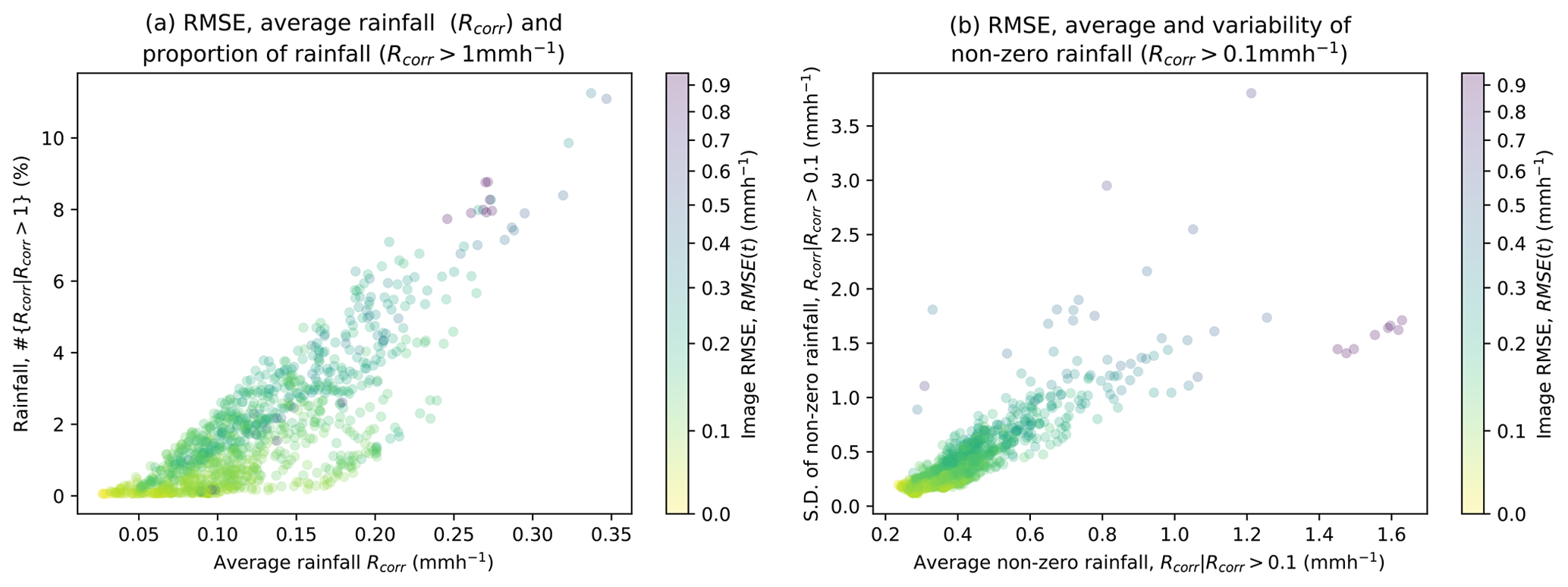
Figure 17 (a) Average rainfall rate and proportion of significant rainfall and (b) average and standard deviation of non-zero rainfall, coloured according to the image RMSE for event images.

Figure 18 shows the average rainfall rate (see Fig. 18a–e) and the proportion of non-zero rainfall (see Fig. 18f–j) in event images for the average bias, RMSE, ARS, PRS and LARS. For higher rainfall rates and proportions of rainfall, the bias increases, with low proportions of low rainfall rates exhibiting a negative average bias. This is also the case for the average non-zero rainfall rates. However, the relationship between the proportion of non-zero rainfall and the RMSE is less distinct, highlighting the significant impact of very small areas of intense rainfall rates on the image's RMSE. Figure 18 also shows that there are some low average rainfall rates and proportions of non-zero rainfall which correspond to high areas of the shadowed rainfall. This may be attributed to noise. However, this does suggest again that events do not need to include intense large-scale rainfall areas to result in significant rainfall shadows. The proportion of shadowed rainfall also appears to increase exponentially as the average non-zero rainfall rate increases, which is not the case with the proportion of rainfall in the images.

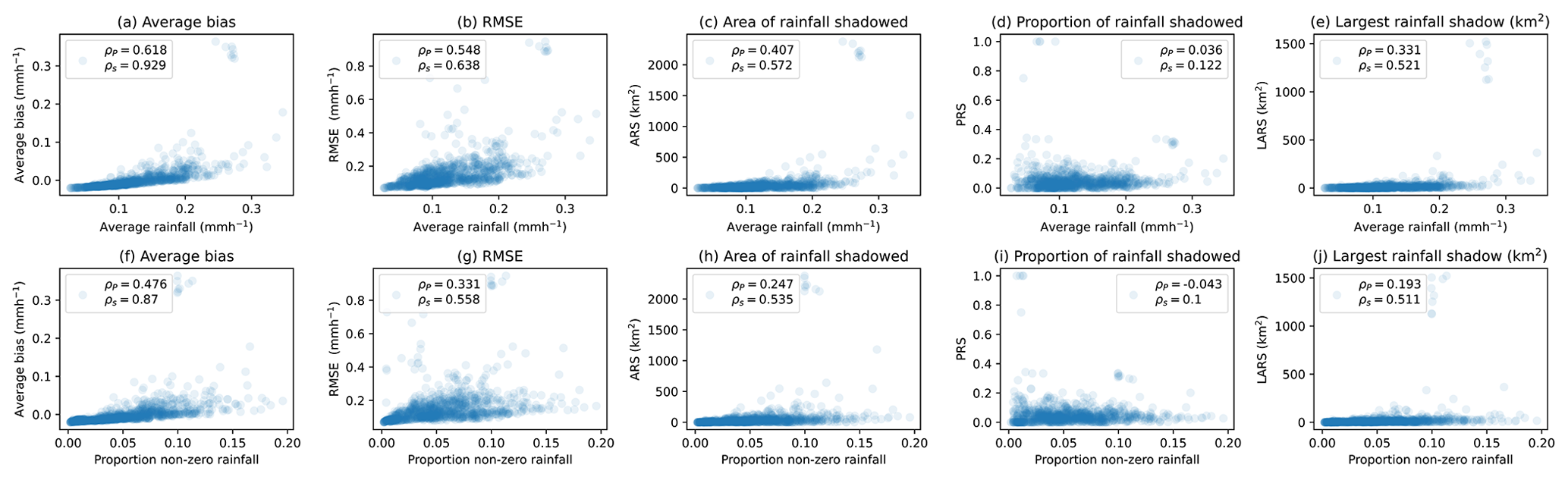
Figure 18 Average rainfall rate (a–e) and proportion of non-zero rainfall (f–j) for metrics including average bias, RMSE, area of rainfall shadowed (ARS), proportion of rainfall shadowed (PRS) and largest rainfall shadow area (LARS) for ensemble images of all events.

The relationships in Fig. 18 are heavily skewed by a high density of images with low average rainfall rates and proportions. For a clearer image of the behaviour for event images, see the average rainfall rates of 0.1, 0.5 and 1 mm h⁻¹ in Fig. 19. This shows a much clearer relationship between the corrected rainfall field and the rainfall shadows, with strong correlations between the average bias and the average rainfall rate (see Fig. 19a, f and k). The relationship becomes less clear for higher rainfall thresholds for conditional averages, with the strongest correlation between the non-zero rainfall average and the RMSE (see Fig. 19b).

Figure 19 Average thresholded rainfall rate for R(t)>0.1 mm h⁻¹ (a–e), R(t)>0.5 mm h⁻¹ (f–j) and R(t)>1 mm h⁻¹ (k–o) for metrics including average bias, RMSE, ARS, PRS and LARS for ensemble images of all events.

Figure 20 Standard deviation of the ensemble bias (a) and RMSE (b) for average non-zero rainfall rates of ensemble images for all events.

From Fig. 19c, h and d, the ARS in the images may increase exponentially with increasing average rainfall rates. However, this may be skewed by the small number of images with very high ARS values (larger than 1000 km²). For the thresholded rainfall rates, most correspond to a low ARS value but appear to increase exponentially, particularly in Fig. 19c. There are some images with low ARS values which have high-threshold rainfall rates, which may be a result of small areas of high-intensity rainfall, where there are no resulting shadows as there are no other areas of significant rainfall rates (R(t)). The relationship between the proportion of rainfall is more complex (see Fig. 19d, i and n), with two distinct types of image behaviour. While a correlation is evident between the conditional average rainfall rates and the PRS values, there is clearly a large number of images with low average rainfall rates and large PRS values. These high PRS values with low average rainfall rates most likely correspond to images with a very low proportion of rainfall rates large enough to be classed as shadows. If just 1 rainfall pixel is shadowed, there would be a large increase in the PRS value in this case, highlighting the impact that shadows have on images with low rainfall extents, with fairly low average rainfall rates.

From Fig. 19e, j and o the LARS values appear to have a similar relationship with the ARS values. However, these are again skewed by very high ARS values, and so the relationship is less clear. Considering that the overall average behaviour of the ensemble does not take full advantage of the model framework and different ensemble member properties, important variation information is lost, which may have increased understanding of the uncertainty associated with the radar rainfall estimation process.

4.7 Individual image-based errors: ensemble variability

The variability between the ensemble members for each event image is considered using the ensemble standard deviation to identify areas where the event errors have a high level of uncertainty in image properties. Figure 20a shows the relationship between the average non-zero rainfall rate and the standard deviation of the image bias, showing rainfall images with an average non-zero rainfall rate of less than 0.5 mm h⁻¹. There is no clear relationship between the average rainfall and variability in the bias of estimates. For images with an average non-zero rainfall rate above 0.5 mm h⁻¹, there appears to be a strong positive correlation between the two, suggesting that, past this image threshold, the uncertainty in the image bias is directly proportional to the average non-zero rainfall rate.

The relationship between the average non-zero rainfall rate and the image's RMSE variability in Fig. 20b is very different, appearing to be inversely proportional to the variability in the image's RMSE. This may be attributed to the fact that, for higher rainfall rates, there are more rainfall shadows. In areas where there are rainfall shadows, the variability between the ensemble members decreases significantly due to the effects of the radar ray signal being fully damped. There is a moderate relationship between the variability PRS and the average non-zero rainfall. However, this is less distinct.

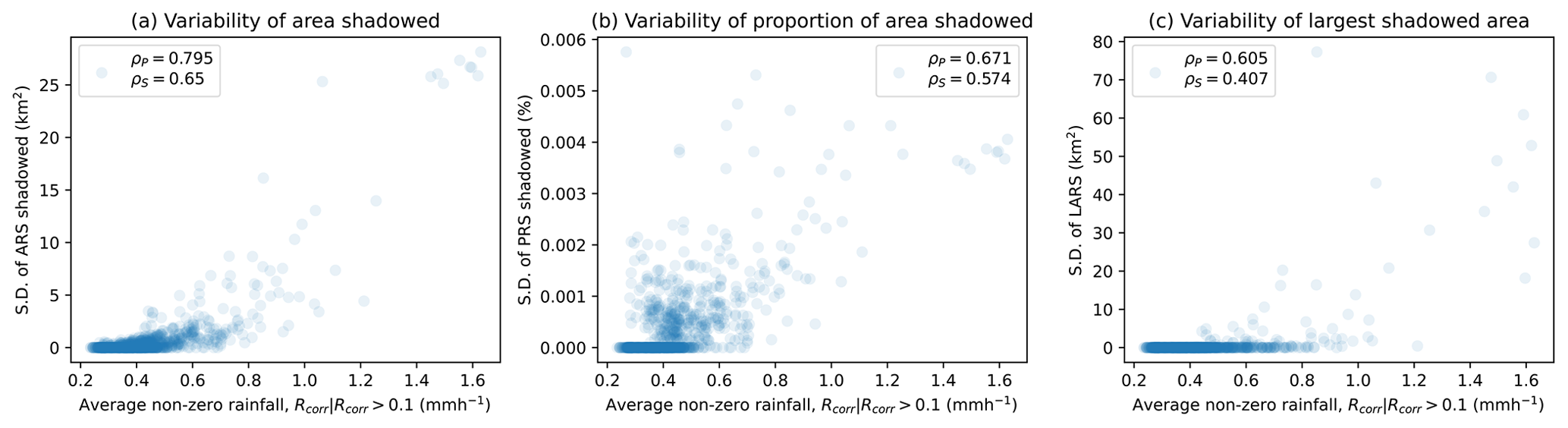
Figure 21 Standard deviation of the ARS (a), PRS (b) and LARS (c) for average non-zero rainfall rates of ensemble images for all events.

The standard deviations of the ARS, PRS and LARS are given in Fig. 21. From Fig. 21a we can see that the uncertainty in the ARS increases with an increasing average rainfall rate, with similar behaviour for the LARS in the images (see Fig. 21c). However, there are a lot of images with no ARS skewing the relationship. Again, the relationship between the average non-zero rainfall rate and the variability of the PRS is not clear (see Fig. 21b).

4.8 Rainfall location: second moment of area

The location of rainfall with respect to the radar location will also impact the error structure, which is reflected in the variability in the PRS for different average rainfall rates. Atlas and Banks (1951) stated that distortion due to range attenuation includes displacement towards the radar of maximum intensity, packing contours on the near side of the storm and suggesting that the location of high-intensity rainfall will also have an impact on errors. The amount of rainfall lost to attenuation effects is likely to be higher for images with high-intensity rainfall in a more central location, due to the cumulative nature of attenuation effects along a radar ray. As illustrated in Fig. 22, the occurrence of rainfall close to the radar transmitter affects more rays, and its attenuation affects more “downstream” pixels. There is evidence of this in Fig. 9, where high-intensity rainfall occurred in the centre of the image, resulting in very high errors.

Figure 22 Schematic of the different effects high-intensity rainfall has on radar rays based on its location within the domain.

To formally investigate this, we introduce the second moment of area of a rainfall (or reflectivity) image, estimated by considering the centroid of each image using the second areal moment. For the rainfall field R(t) on a Cartesian grid with dimensions (N_x, N_y), the second moment of area can be estimated as

$$\begin{array}{}\text{(13)}& \begin{array}{rl}{M}_{\mathrm{R}}\left(t\right)& =\sum _{x=\mathrm{1}}^{N_x}\sum _{y=\mathrm{1}}^{N_y}R(x,y,t)d(x,y{)}^{\mathrm{2}}\\ & =\sum _{x=\mathrm{1}}^{N_x}\sum _{y=\mathrm{1}}^{N_y}R(x,y,t)\left\{{\left(x-r_x\right)}^{\mathrm{2}}+{\left(y-r_y\right)}^{\mathrm{2}}\right\},\end{array}\end{array}$$

where $d(x,y)=\sqrt{(x-r_x{)}^{\mathrm{2}}+(y-r_y{)}^{\mathrm{2}}}$ is the distance of a pixel from the radar location (r_x, r_y). Both the actual and normalized rainfall fields are used to see the different impacts between the shapes of the field, with and without considering the actual magnitudes of the estimates. The normalized image moments ${\stackrel{\mathrm{̃}}{M}}_R\left(t\right)$ are defined as

$$\begin{array}{}\text{(14)}& {\stackrel{\mathrm{̃}}{M}}_{\mathrm{R}}\left(t\right)=\sum _{x=\mathrm{1}}^{N_x}\sum _{y=\mathrm{1}}^{N_y}{\displaystyle \frac{R(x,y,t)}{R_{\mathrm{tot}}\left(t\right)}}\left\{{\left(x-r_x\right)}^{\mathrm{2}}+{\left(y-r_y\right)}^{\mathrm{2}}\right\},\end{array}$$

where $R_{\mathrm{tot}}\left(t\right)=\sum _x\sum _{y}R(x,y,t)$ is the total rainfall (R(t)).

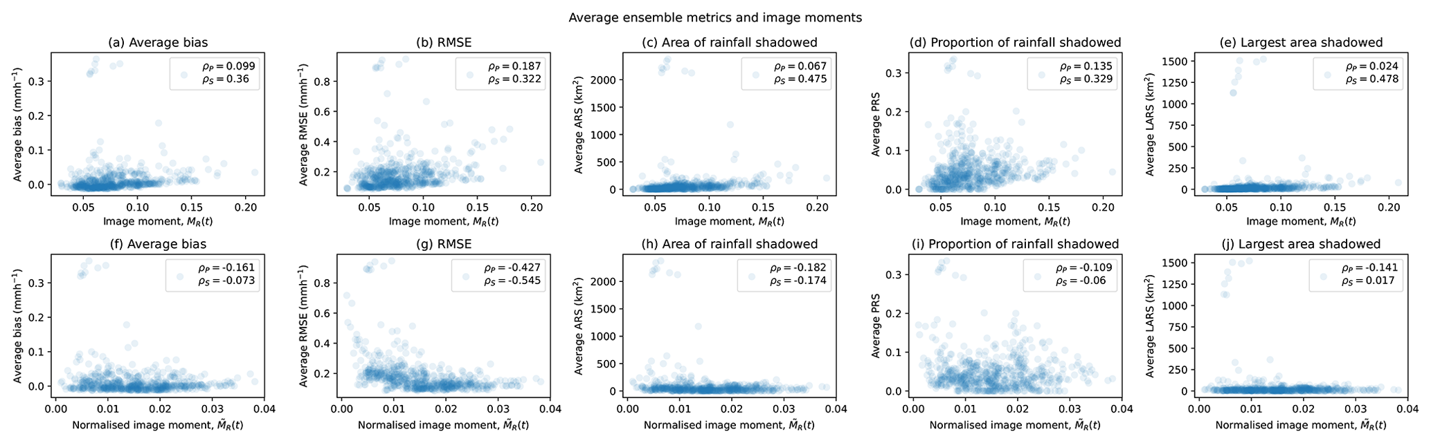
Figure 23 Second moment of area (a–e) and normalized second moment of area (f–j) for metrics including average bias, RMSE, ARS, PRS and LARS for ensemble images of all events.

Figure 23 shows the relationship between the second moment of area M_R(t) and the normalized second moment of area ${\stackrel{\mathrm{̃}}{M}}_{\mathrm{R}}\left(t\right)$ for event images and corresponding ensemble metrics including the average bias, RMSE, ARS, LARS and PRS. There are significant differences between the moments and normalized moments, with positive correlations for image moments and an inverse relationship for normalized image moments, which is particularly prominent when considering the RMSE. There is a significant positive correlation between image moment and RMSE, ARS and PRS, with the relationship for LARS being less clear.

Figure 24 Second moment of area (a–e) and normalized second moment of area (f–j) for ensemble metric variability (standard deviation), including average bias, RMSE, ARS, PRS and LARS for ensemble images.

This suggests that, for the second moment of area calculated on rainfall rates, the strong non-linear dependence on absolute rainfall amount overrides all other information on the field, such as rainfall location. For the normalized second moment of area, this dependence has been removed, and so the relationship is solely based on the impact of the rainfall location. In this case, a smaller second moment of area (corresponding to a more central rainfall location) suggests larger rainfall shadows.

Figure 24 shows the relationship between the second moment of area and the normalized second moment of area for events, together with the ensemble uncertainty for the image metrics given in Fig. 23. This shows that images with a larger image moment have a lower RMSE standard deviation. The normalized image moments appear to be positively correlated with the standard deviation of the bias and RMSE and negatively correlated with the ARS, PRS and LARS. The variability in rainfall shadows, for both the ARS and PRS, appears to decrease with increasing normalized image moments.

Image moments could be a key piece of information when attempting to identify radar images with high uncertainty in estimates, particularly when using moments calculated from normalized rainfall rates across an image. In conclusion, this analysis suggests that a second moment of area has the potential to identify high uncertainty and missing information.

4.9 Rainfall shadow frequency

The aim of this section is to identify how often rainfall shadows occur. Due to ensemble variability, to ensure that frequencies are not overestimated, we consider the “best-case scenario” over the ensemble. In terms of the ensemble, for each image the ensemble member with the lowest errors is selected. This prevents overestimation, and as rainfall fields are parameterized with existing corrected radar rainfall images that may themselves be subject to rainfall shadows, the simulations may inherently underestimate the frequencies, so considering the minimum likelihood of occurrence makes intuitive sense. Percentiles are given for the minimum LARS, PRS and ARS in Table 1.

Table 1 Percentiles for the empirical cumulative distribution functions (ECDFs) for the minimum ensemble rainfall shadow proportions, largest shadowed areas and actual rainfall shadowed for all events.

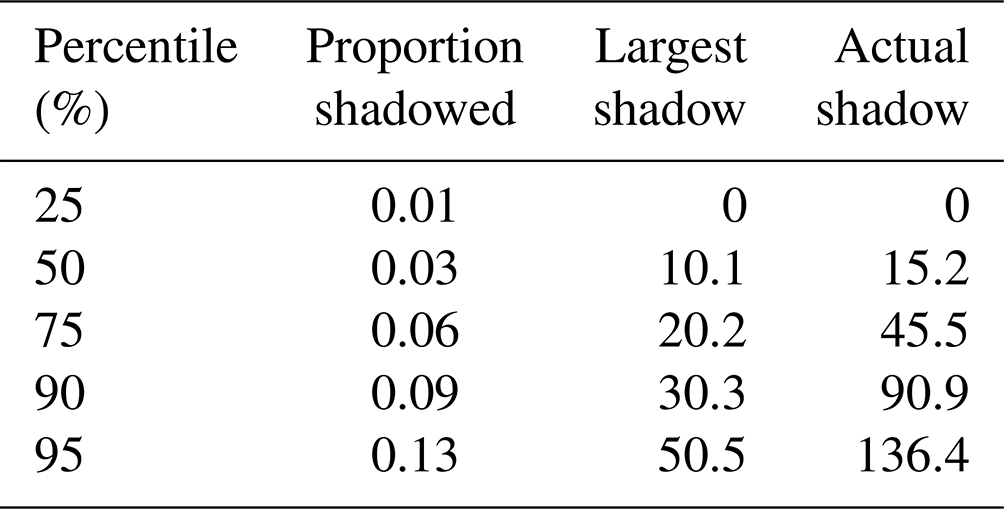
The empirical cumulative distribution functions for the minimum LARS, PRS and ARS are estimated for simulated events, with attenuation estimated from rainfall and reflectivity and given in Fig. 25. From the median of the proportion of the rainfall images simulated, half of the images have at least 3 % of their significant rainfall rates shadowed. When considering the ARS in the images, we see that 25 % of the images have an ARS of 45 km² and that 5 % have a LARS of over 50 km². A missing area of significant rainfall of this size, particularly for small or urban catchments, constitutes a major underestimation of flood risk, resulting in incorrect information provided in flood warnings. This highlights the importance of gaining an improved understanding of rainfall shadows and provides a motivation for this project and future research in this area. Gaps caused by the rainfall shadows identified would result in underprediction of flooding, impacting both flood warnings and flood defence designs.

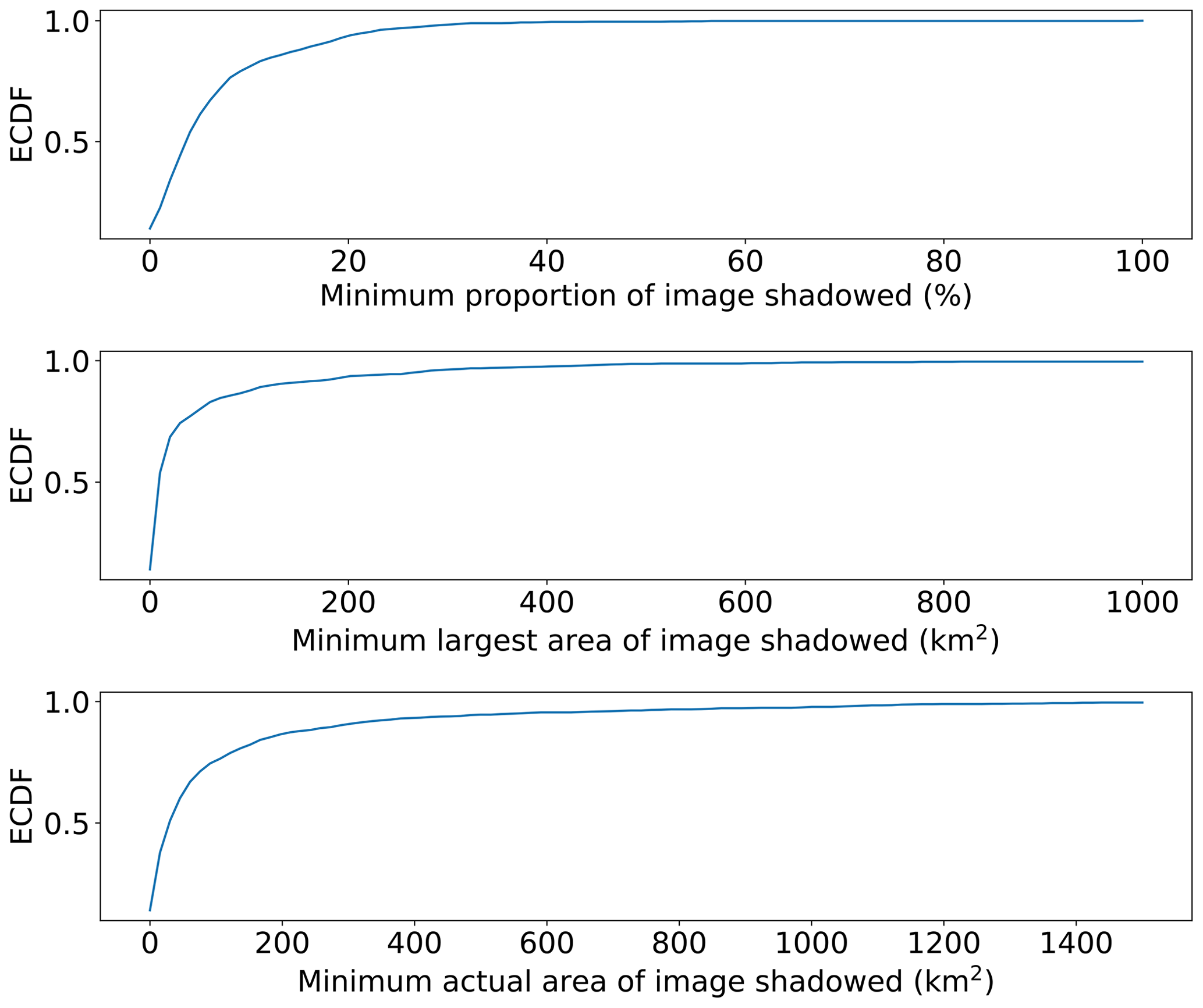
Figure 25 Empirical cumulative distribution functions (ECDFs) for the minimum ensemble proportion, together with the largest and actual areas of image-containing rainfall shadows for all events.

5 Discussion and conclusions

Errors relating to several different aspects of the radar rainfall estimation process are considered, using a radar error model outlined in detail. This model is applied to realistic simulated rainfall events in a stochastic manner, generating an ensemble of radar images corresponding to each time step of a rainfall event. A log-normal random noise field was imposed on rainfall estimates to account for underlying non-specific noise. The DSD uncertainty is included by replacing the multiplicative parameter a in the Z–R relationship with a two-dimensional spectral random field, with field variability determined by radar sampling volumes. Attenuation effects are imposed by inverting standard gate-by-gate correction algorithms (Jacobi and Heistermann, 2016). To enable direct comparison between the simulated rainfall before and after imposing the radar error model, each radar image is corrected using a standard radar rainfall estimation process. This results in a corrected rainfall field for each ensemble member, similar to what would be obtained from real radar rainfall images, allowing us to identify when and where significant and/or systematic errors may occur.

This concept provides a methodology for developing a better understanding of errors related to the radar rainfall estimation process. By generating a true rainfall field and subsequently imposing errors to allow for comparison with correct best-guess stochastic radar rainfall estimates, we can address the fundamental limitation of weather radar correction schemes – that the real rainfall field is not known for comparison. An investigation of the spatio-temporal behaviour of the error structure is then possible, which provides key information on the radar rainfall estimation process.

A relationship between rainfall shadows, high bias and uncertainty related to the amount of rainfall (i.e. proportions and rates) in images was found. The impact of the rainfall location with respect to the weather radar is considered by introducing the second moment of area, showing that more central rainfall in the radar domain results in higher errors and variability. The minimum likelihood of rainfall shadows showed that 50 % of the simulated images have at least 3 % of their significant rainfall shadowed. In addition, 25 % of the images had an ARS of over 45 km², with the minimum LARS of 5 % of the images exceeding an area of 50 km². This gap would result in underestimation of potential impacts of flooding. This highlights the importance of gaining an improved understanding of rainfall shadows and provides the motivation for this project and future research in this area. Weather radar alone cannot be used for rainfall estimation, as information is regularly missed.

5.1 Impact and transferability

Improved high-resolution rainfall estimates are needed for flood forecasting by stakeholders and water managers, particularly in (near) real time, for nowcasting and probable ensemble forecasting. The radar error model outlined in this study produces visually realistic radar images, capturing key properties of radar images, with many potential uses for the model framework, some of which are outlined below:

1. Identification of radar rainfall properties which correspond to high errors and uncertainties could be extended and used in a probabilistic manner to better condition merged rainfall fields. Identify areas where the spatial distribution of the rainfall cannot be trusted (i.e. occasions where rainfall shadows are likely, such as areas past high-intensity rainfall). This includes information on the frequency and location of rainfall shadows as a merging criterion (i.e. putting more weight on rainfall information from other sources when rainfall shadows are likely to occur at a given location).

2. Apply the model to gridded rain gauge fields or forecasts, for comparison with the corresponding weather radar images, to better identify and understand radar rainfall errors.

3. The importance of complex and efficient radar gauge merging methods is emphasized in this study. These methods do not trust the spatial distribution of rainfall provided by weather radars alone. Additional information from other sensors is needed, such as opportunistic sensors, citizen science data, rain gauges and microwave links. This study has provided a framework for methods assessing the performance of these merging techniques.

4. Determine the optimal locations for weather radars or rain gauges, such as establishing rain gauge networks in areas where rainfall shadows are more likely and not in densely populated areas (e.g. cities), where it may be too late for warnings on missing information.

5. Assess how radar rainfall errors propagate into hydrological and hydrodynamic modelling, considering the impact that the incorrect distribution of rainfall has on discharge and flood depths.

5.2 Limitations and future work

A powerful framework for investigating radar rainfall errors has been developed and demonstrated, with model design allowing for a high degree of flexibility and several natural extensions. The influence of different correction methods for the radar rainfall estimation process and the impact this has on the error structure should be investigated using the methodology in this study.

Some error sources in radar rainfall estimation are not included in the radar error model, as they were beyond the scope of this study. To improve the model, additional sources of error could easily be included (e.g. radar calibration errors using an additive error (dBZ) and bright-band effects using a vertical representation of different weather types and seasons of events). Mountainous regions are typically subject to more errors due to beam blockage from topography. However, this could quite easily be included in the model through an additive error based on existing clutter maps from the weather radar of interest. It would be interesting to repeat the study with different DSD structures, changing the correlation structure and marginal distribution of this (previously Gaussian) field. A dependence between DSD parameters could be imposed, as a varying Z–R relationship in space and time improved rainfall accumulations at the event scale (Libertino et al., 2015).

Close to the radar, measurement volumes are small, systematically increasing in size with distance from the radar. Although as part of the radar error model the spatial sampling aspect is considered through the estimation variance, radar measurements are taken to be instantaneous (as opposed to rain gauge measurements, which are temporal aggregations by definition). The implications of these space–time sampling properties mean that temporally we only have a snapshot of the pixel behaviour at a given time. Correlation structure variability in space and time was incorporated through a spatio-temporal anisotropy factor, without explicitly accounting for the different data sampling between the two dimensions. The simulation environment could be modified to account for the temporal sampling issue by simulating temporally at a higher resolution than existing radar images and sampling these to reproduce the snapshot effect. Methods could also be developed within an inverse modelling framework (Grundmann et al., 2019) to obtain field uncertainty in (near) real time.

5.3 Concluding remarks

The overarching aim of this study is to contribute towards improvements in the radar rainfall estimation process by gaining an improved understanding of the frequency and location of the error structure relating to the process. With this in mind, we explore and exploit space–time properties of rainfall and reflectivity to gain an improved understanding of the error structure between the two, investigating the extent of uncertainties in the radar rainfall estimation process. This study has presented an innovative model for investigating uncertainties in the radar rainfall estimation process, providing a flexible tool that has many potential future applications. The radar error model, outlined in detail, generates a stochastic ensemble of radar images corresponding to an existing rainfall field by inverting the radar rainfall estimation process. This model incorporates many different error sources, including the drop-size distribution, attenuation effects, random noise and radar sampling. This provides a method for identifying when and where radar errors are likely to occur and how often information about the rainfall field is lost, significantly impacting the spatial rainfall field. The insights from this study provide an improved understanding of the error structure between rainfall and reflectivity, together with the extent of uncertainties in the radar estimation process. A framework has been provided to investigate the impact of errors relating to the radar rainfall estimation process, with many potential hydrological applications.