Characterizing nonlinear, nonstationary, and heterogeneous hydrologic behavior using ensemble rainfall–runoff analysis (ERRA): proof of concept

A classical approach to understanding hydrological behavior is the unit hydrograph and its many variants, but these often assume linearity (runoff response is proportional to effective precipitation), stationarity (runoff response to a given unit of rainfall is identical, regardless of when it falls), and spatial homogeneity (runoff response depends only on spatially averaged precipitation). In the real world, by contrast, runoff response is typically nonlinear, nonstationary, and spatially heterogeneous. Quantifying this nonlinearity, nonstationarity, and spatial heterogeneity is essential to unraveling the mechanisms and subsurface properties controlling hydrological behavior.

Here, I present proof-of-concept demonstrations illustrating how nonlinear, nonstationary, and spatially heterogeneous rainfall–runoff behavior can be quantified, directly from data, using ensemble rainfall–runoff analysis (ERRA), a data-driven, model-independent method for quantifying rainfall–runoff relationships across a spectrum of time lags. I show how ERRA uses nonlinear deconvolution to quantify how catchments' runoff responses vary with precipitation intensity and to estimate their precipitation-weighted runoff response distributions. I further illustrate how ERRA combines nonlinear deconvolution with de-mixing techniques to reveal how runoff response depends jointly on precipitation intensity and nonstationary ambient conditions, including antecedent wetness and vapor pressure deficit. I demonstrate how ERRA's de-mixing techniques can be used to quantify spatially heterogeneous runoff responses in different parts of a catchment, even if those subcatchments are not separately gauged. I also illustrate how ERRA's broken-stick deconvolution capabilities can be used to quantify multiscale runoff responses that combine hydrograph peaks lasting for hours and recessions lasting for weeks, well beyond the average spacing between storms.

ERRA can unscramble these multiple effects on runoff response even if they are overprinted on each other through time and even if they are corrupted by autoregressive moving average (ARMA) noise. Results from this approach may be informative for catchment characterization, process understanding, and model–data comparisons; they may also lead to a better understanding of storage dynamics and landscape-scale connectivity. An R script is provided to perform the necessary calculations, including uncertainty analysis.

1 Introduction

1.1 Response time versus transit time

When a substantial rainstorm hits a catchment, streamflow will often rise, peak, and recede within a matter of hours or days. However, much of the rainwater from that storm will remain within the catchment for months or even years, affecting the composition of streamflow long after the storm's effects on discharge rates have faded away. Therefore, streamflow often primarily consists of precipitation that fell long ago but is primarily mobilized by rain that fell much more recently. Thus, timescales of hydrologic response are often much shorter than timescales of transport. This decoupling of timescales has been recognized since at least the 1960s (e.g., Brown, 1961; Martinec, 1975; Rodhe, 1981), but it has been widely overlooked in hydrology textbooks and rainfall–runoff models, and understanding its underlying mechanisms remains a central challenge in catchment hydrology (Kirchner, 2003; Beven, 2012; McDonnell and Beven, 2014).

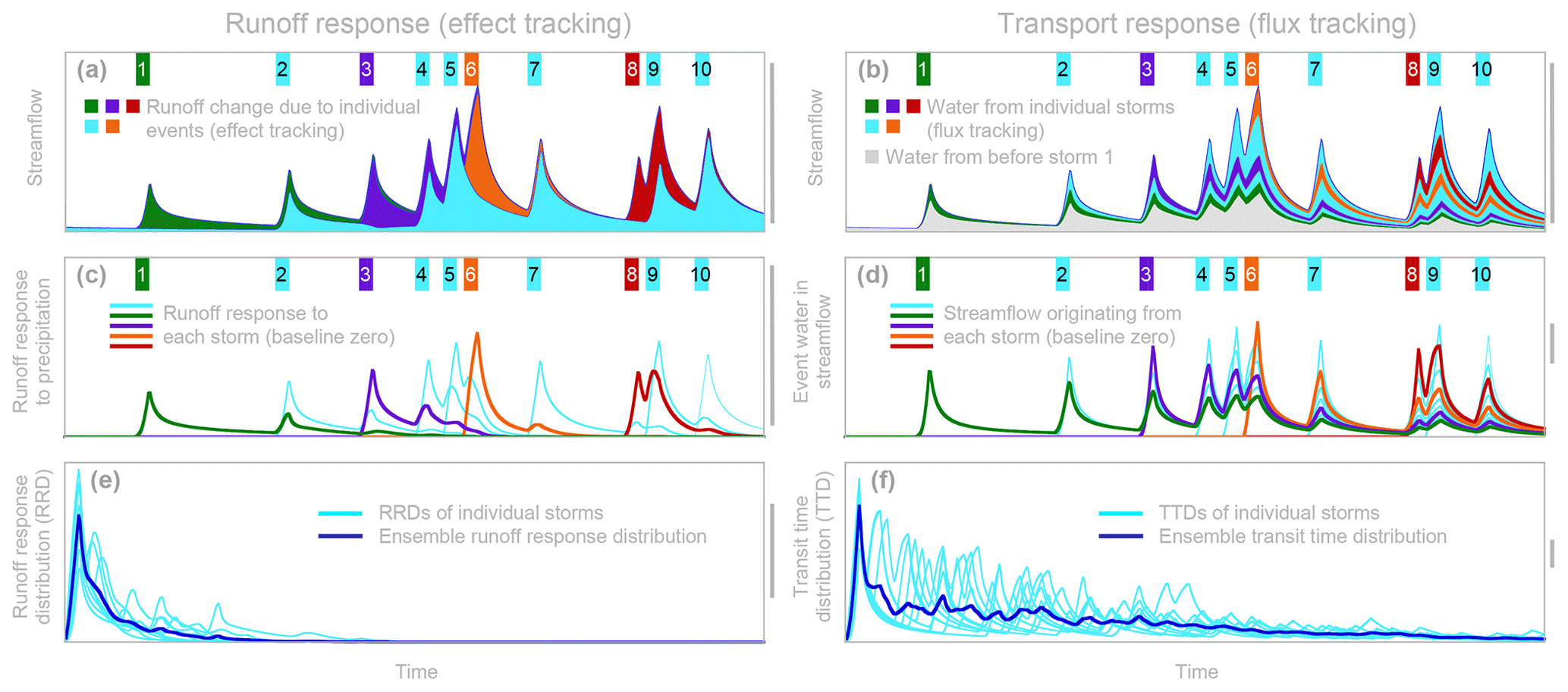
Figure 1 Effects of 10 rainstorms on future runoff (a, c, and e) compared to future streamflow composition (b, d, and f), illustrated using the nonlinear two-box benchmark model of Kirchner (2019). In (a), the colored bands show the runoff response to the corresponding storms, as determined by effect tracking. Effect tracking quantifies the runoff response according to how much the discharge time series changes when individual storms are included in or excluded from the precipitation time series. Thus (for example) the orange domain shows how much more runoff occurred when storm no. 6 was included in the precipitation time series versus when it was excluded (shown by the teal-colored hydrograph). In (b), the colored bands show the streamflow fluxes that originated as precipitation during each storm, as determined by flux tracking (streamflow from precipitation that fell before event no. 1 is shown in gray). Panels (c) and (d) show the runoff and transport responses, respectively, for all 10 storms, plotted against a baseline of zero so that they can be more clearly compared. Panels (e) and (f) show the same curves, expressed as the time since the start of their respective storms. Dark-blue curves show the ensemble-averaged runoff response distribution (RRD, panel e) and transit time distribution (TTD, panel f). Each horizontal axis shows the same time interval. The vertical scales are identical in panels (a–c) but differ among the remaining panels to more clearly show the behavior. The gray bars along the right edge of each panel show what the relative sizes of the vertical axes would be if the scales were consistent. Model parameters are S_u,ref = S_l,ref = 400 mm, b_u = b_l = 10, and η = 0.5. Each of the 10 modeled storms are of equal intensity (20 mm h⁻¹) and duration (10 h). The model ignores evapotranspiration so each 200 mm storm causes 200 mm of additional streamflow in the future (a) and adds 200 mm of water that will eventually leave the catchment (b). Thus, the total volumes of the colored bands in (a) and (b) are equivalent, but the hydrological response to precipitation (a, c, and e) decays away much faster than the event water is flushed out of the catchment (b, d, and f). Modified, with permission, from Kirchner et al. (2023). Permission for the re-use and/or modification of this figure can be found at the following link: https://www.annualreviews.org/page/authors/author-instructions/distributing/permissions (last access: 7 August 2024).

The contrast between hydrologic response and transport, and between their respective timescales, can be simply illustrated through the behavior of a simple conceptual catchment model. Figure 1 shows how a simple nonlinear two-box model responds to a hypothetical sequence of 10 identical rainstorms (Kirchner et al., 2023). The left-hand side of Fig. 1 shows how each rainstorm affects future discharge rates, whereas the right-hand side shows how much water from each rainstorm is present in future streamflow. Four individual storms are highlighted in contrasting colors.

The effects of each event on future runoff volumes are quantified by effect tracking – that is, by running the model with and without each event and then comparing the resulting hydrographs. The differences between the hydrographs with and without the four highlighted rainstorms, which quantify the stream's runoff response, are shown by the matching colored bands in Fig. 1a. The runoff responses to all 10 storms are shown in Fig. 1c, each expressed relative to a baseline of zero so that their magnitudes can be more easily compared.

One can see that, owing to the nonlinearities in the underlying model, the runoff responses that are initially larger decay away faster. One can also see that the initial runoff responses are larger for storms that fall when the model catchment is already wet, and, thus, discharge is already high; because the model is nonlinear, runoff response to a given storm depends on how large and how recent previous storms were. The model's nonlinearity further implies that runoff response also depends on future precipitation, as one can see from Fig. 1c. In one particularly clear example, the largest runoff response to storm no. 8, shown in red, does not come at the end of storm no. 8 but instead comes during storm no. 9, illustrating how storm no. 9 amplifies storm no. 8's effects. When these runoff response curves are synchronized according to the times that the precipitation fell and are normalized by the precipitation rate (Fig. 1e), they can be considered to be runoff response distributions (RRDs), which quantify how the runoff response to a unit of precipitation is distributed over future time. In nonlinear systems, these runoff response distributions will be time-varying because they depend on the size and timing of both preceding and subsequent precipitation inputs, as shown in Fig. 1e. Nonetheless, one may summarize the time-varying RRDs for a given ensemble of events by averaging them together, resulting in the ensemble runoff response distribution shown in dark blue in Fig. 1e. Estimating this ensemble-averaged response directly from data is the central task of this paper.

In contrast to the short-lived runoff response shown on the left-hand side of Fig. 1, the right-hand side shows that the same storms have much more persistent effects on the composition of streamflow itself (compare Fig. 1a and b). Figure 1d shows the contributions of all 10 storms to future streamflow, relative to a baseline of zero so that they can be more easily compared (analogously to Fig. 1c). Storms that fall when the catchment is wetter generate sharper peaks in Fig. 1d and also mobilize more water from prior storms compared to storms that fall during drier conditions. Therefore, each storm's distribution of transit times (between when water enters the catchment and subsequently leaves it) depends on the size and timing of both previous and subsequent storms. Thus, these transit time distributions (TTDs; light-blue curves in Fig. 1f) are time-varying, but they can, nonetheless, be summarized by averaging them over an ensemble of events, resulting in the ensemble transit time distribution shown in dark blue in Fig. 1f.

The behaviors shown in Fig. 1 are not data; instead, they are hypothetical results derived from a particular simulation model for purposes of illustration. Are these results, nonetheless, at least qualitatively relevant to the real world? In the early days of scientific hydrology, the observed rapid response of runoff to rainfall led to an intuitive assumption that storm hydrographs should be mostly composed of “new” water from recent rainfall traveling quickly to the stream, often via overland flow (Horton, 1933). This conceptual model formed the foundation of decades of unit hydrograph studies (beginning with the work of Sherman, 1932), as well as attempts to relate the unit hydrograph to drainage basin geomorphology (e.g., Ross, 1921; Rodriguez-Iturbe et al., 1982; Gupta et al., 1980), as reviewed by Rigon et al. (2015) and Beven (2020). The assumption that recent rainfall dominates storm hydrographs was subsequently challenged by tracer data showing that streamflow, even during storm peaks, is often composed mostly of “old” water from precipitation that fell much earlier (e.g., Brown, 1961; Hubert et al., 1969; Martinec, 1975; Pinder and Jones, 1969; Sklash and Farvolden, 1979; Rodhe, 1981; Sklash, 1990; Neal and Rosier, 1990). This discovery has spurred decades of studies using isotopes and conservative chemical tracers to estimate transit times in many different catchments (e.g., Kirchner et al., 2000; McGuire and McDonnell, 2006; Godsey et al., 2010; Botter et al., 2010; van der Velde et al., 2012; Heidbüchel et al., 2012; Benettin et al., 2015a, b, 2022; Harman, 2015; Berghuijs and Kirchner, 2017; Kirchner, 2019; Knapp et al., 2019).

Amid the intense focus in recent decades on catchment travel times and on flux tracking in models (e.g., the right-hand side of Fig. 1), questions of catchment response times, and of effect tracking in models (e.g., the left-hand side of Fig. 1) have received much less attention. As a step toward addressing this imbalance, this paper presents ensemble rainfall–runoff analysis (ERRA), a model-independent, data-driven method for quantifying runoff response distributions from precipitation and streamflow time series. This approach is made possible by recent mathematical developments in the estimation of impulse response functions for nonlinear, nonstationary, and heterogeneous systems (Kirchner, 2022, hereafter denoted as K2022). ERRA characterizes hydrologic behavior using runoff response distributions (as shown on the left-hand side of Fig. 1) as a counterpart to ensemble hydrograph separation (Kirchner, 2019; Kirchner and Knapp, 2020), which characterizes transport behavior using transit time distributions (as shown on the right-hand side of Fig. 1).

1.2 ERRA versus unit hydrographs

At its core, ensemble rainfall–runoff analysis is based on least-squares deconvolution of a stream discharge time series by one or more precipitation time series. ERRA's heritage thus reaches back to unit hydrograph methods, which have a long history in hydrology (e.g., Sherman, 1932; Snyder, 1955; Dooge, 1973; Bruen and Dooge, 1992). It differs from conventional unit hydrograph approaches in several important ways, however. First, classical unit hydrograph methods invoke what Hewlett and Hibbert (1967) termed “completely arbitrary” assumptions in order to separate the hydrograph into storm runoff and baseflow, and they invoke further assumptions to separate the rainfall time series into effective precipitation and evaporative losses. To avoid making such assumptions, which substantially influence the resulting unit hydrographs (Beven, 2012), ERRA analyzes time series of total precipitation (instead of effective precipitation alone) and total discharge (instead of storm runoff alone). Second, the area under conventional unit hydrographs is constrained to be equal to 1, thus enforcing the assumption that whatever is defined as storm runoff must equal, on average, whatever is defined as effective precipitation (and making the analysis vulnerable to biases in either of these quantities). ERRA makes no such assumption and instead allows the area under the runoff response distribution to reflect mass imbalances due to evapotranspiration losses or infiltration to deep groundwater (or due to potential biases in discharge and precipitation measurements). Third, in contrast to many unit hydrograph methods, ERRA does not require the definition and isolation of individual events but instead assimilates information from the entire time series of precipitation and streamflow. That is, it analyzes how streamflows at every point in time (not just during pre-defined “events”) are correlated with precipitation – or lack thereof – over previous time steps. In this way, it can exploit the information contained in the differences in streamflows that follow different precipitation patterns, including those that follow no precipitation at all. Indeed, a key objective of ERRA is to quantitatively understand how differences in precipitation patterns and ambient conditions shape the relationship between precipitation and subsequent streamflows. Fourth, whereas unit hydrograph methods primarily seek to predict storm hydrographs, ERRA does not focus on hydrograph prediction per se but rather focuses on characterizing the magnitude and timing of rainfall–runoff relationships and on quantifying how they depend on precipitation intensity, ambient conditions, and catchment characteristics. That is, its goal is primarily data-based characterization of hydrologic response rather than prediction of the hydrograph per se.

Fifth, and perhaps most importantly, whereas conventional unit hydrograph methods assume that the effects of rainfall on runoff are linear, stationary, and homogeneous, ERRA is specifically designed to characterize and quantify the nonlinearity, nonstationarity, and heterogeneity of runoff response. For example, typical unit hydrograph methods are driven by a single whole-catchment precipitation time series and thus implicitly assume either that the same precipitation falls everywhere or that its effects on runoff are spatially homogeneous (but there are exceptions, e.g., Kothyari and Singh, 1999). By contrast, through a combination of deconvolution and de-mixing methods, ERRA can distinguish and quantify how runoff responds to precipitation falling on different parts of the landscape, even when those individual hydrologic responses are overprinted on one another at the catchment outlet (see Sect. 2.3 below and Sect. 3 of K2022). Unit hydrograph methods are also based on the premise of linear superposition of precipitation inputs, such that the response to x units of rain falling at time t is assumed to be x times the response to a single unit of rainfall at time t. By contrast, ERRA recognizes that streamflow may respond nonlinearly to variations in rainfall intensity and uses nonlinear deconvolution methods to quantify that response (see Sect. 3 below and Sect. 5 of K2022). Furthermore, conventional unit hydrograph methods assume that runoff response is stationary such that a given unit of rain always has the same effects on runoff, regardless of when it falls. By contrast, ERRA combines deconvolution and de-mixing methods to explicitly quantify how runoff responses vary over time or vary with ambient conditions, even if those runoff responses are overprinted on one another (see Sect. 5 below and Sect. 4 of K2022).

Here, I briefly introduce ERRA and outline some of its potential applications. The mathematical foundations underlying ERRA have previously been documented and benchmark-tested in K2022, and those results will only be briefly summarized here. Instead, the purpose of the present contribution is to outline several applications through proof-of-concept demonstrations, thus illustrating the potential of the technique. Software is provided to perform the necessary calculations, including uncertainty analysis, in the open-source programming environment R.

2 Characterizing spatially heterogeneous hydrological responses via deconvolution and de-mixing

2.1 Runoff response distributions (RRDs) as measures of hydrological response

In their simplest forms, runoff response distributions like the dark-blue curve in Fig. 1e can be interpreted as convolution kernels that, when convolved with precipitation, yield streamflow. In continuous time, this convolution can be expressed as

$$\begin{array}{}\text{(1)}& Q\left(t\right)=\underset{\mathit{\tau }=\mathrm{0}}{\overset{\mathrm{\infty }}{\int }}\text{RRD}\left(\mathit{\tau }\right)P(t-\mathit{\tau })\mathrm{d}\mathit{\tau },\end{array}$$

where Q and P are the rates of streamflow and precipitation, respectively, and the runoff response distribution RRD quantifies their coupling at lag time τ. The process of estimating RRD(τ) from time series of Q and P is termed deconvolution. For typical hydrological time series measured in discrete time steps of length Δt, Eq. (1) becomes

$$\begin{array}{}\text{(2)}& Q_j=\sum _{k=\mathrm{0}}^m{\text{RRD}}_k{P}_{j-k}\mathrm{\Delta }t,\end{array}$$

where Q_j is streamflow at time step j, P_j−k is precipitation occurring k time steps earlier, RRD_k is the impulse response of streamflow to precipitation at lag k, and m is the maximum lag being considered. It is important to keep in mind that, in ERRA, Eq. (2) is applied over large ensembles of time steps j. As explained in Sect. 1.2 above, no attempt is made to isolate individual events for analysis. To estimate the runoff response distribution, it would appear to be straightforward to re-cast Eq. (2) as the multiple linear regression equation shown below:

$$\begin{array}{}\text{(3)}& Q_j=\sum _{k=\mathrm{0}}^m{\mathit{\beta }}_k{P}_{j-k}+\mathit{\alpha }+{\mathit{\epsilon }}_j,\end{array}$$

(see also Eq. 4 of K2022) where RRD_k is estimated by ${\mathit{\beta }}_k/\mathrm{\Delta }t$, the constant term α accounts for persistent biases or mass imbalances, and the residuals ε_j capture any time-varying errors. However, conventional least-squares regression techniques assume that the residuals ε_j are temporally uncorrelated white noise, whereas, in practice, streamflow estimation errors typically have both autoregressive and moving-average characteristics. These autoregressive moving-average (ARMA) errors can arise from several sources. Measurement errors in discharge may be serially correlated. There will also be measurement errors in precipitation, and even if they are not themselves serially correlated, they will be smoothed and lagged by the same convolution process that smooths and lags the (unknown) true precipitation, leading to correlations in the residuals. Misspecification of the underlying model, such as its assumption of linearity and stationarity (these assumptions are relaxed later), will also be reflected in serial correlations in the residuals ε_j. Deconvolution in the presence of such ARMA residuals is a non-trivial problem because the fitted streamflow values will contain serially correlated signals both from the errors ε_j and from the real-world process that convolves precipitation to generate streamflow, and these signals need to be distinguished from one another. It is even more challenging to perform such deconvolutions efficiently in large problems, which may involve hundreds of thousands of time steps and hundreds or even thousands of lag times. Readers are referred to Sect. 2 of K2022 for technical details of how this is done and for benchmark tests demonstrating that ERRA handles this challenge effectively and efficiently (i.e., over 3 orders of magnitude faster than the closest built-in R function). ERRA implements this correction for ARMA noise by default, with no intervention required by users in most circumstances (for an earlier implementation of an analogous approach, see Duband et al., 1993). Because this approach is based on solving large linear regression problems and then deconvolving the resulting coefficients, the standard errors of the RRD coefficients can be straightforwardly calculated from the normal equations of regression, combined with first-order, second-moment error propagation for any transformations of the coefficients themselves (see Sects. 2.3 and 5.1 of K2022 for details). ERRA reports the resulting standard errors with all of its outputs.

One technical detail that is particular to hydrology, and thus not covered in K2022, is that the effective lag time between precipitation and streamflow, along with the value of RRD_k at lag k=0, will depend on whether Q_j is the instantaneous streamflow at the end of time step j or the average streamflow over time step j. If Q_j is measured instantaneously at the end of each time step, the average lag between rainfall and its effect on streamflow is (k+0.5)Δt and ${\text{RRD}}_k={\mathit{\beta }}_k/\mathrm{\Delta }t$ for all k. However, if Q_j is averaged over each time step, during lag step zero (k=0), streamflow will only reflect the effects of rain that falls beforehand and not later during the same time step. Thus, streamflow at the end of the time step will reflect all of the rain that fell during that time step, while streamflow at the beginning of the time step will reflect none, and streamflow in the middle of the time step will reflect half (on average since rainfall is stochastic). Integrating over stochastic rainfall fluctuations in many such time steps will yield the result that, when lag k=0, β_k=0 is reduced by half; thus, the RRD must be estimated as ${\text{RRD}}_{k=\mathrm{0}}=\mathrm{2}{\mathit{\beta }}_{k=\mathrm{0}}/\mathrm{\Delta }t$, and the average lag time linking the effects of precipitation to streamflow is $\mathrm{\Delta }t/\mathrm{3}$. For lags k>0, ${\text{RRD}}_k={\mathit{\beta }}_k/\mathrm{\Delta }t$, and the effective lag time is kΔt.

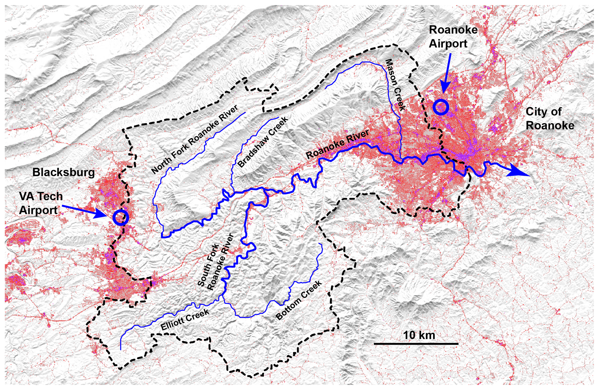
Figure 2 Map of the 995 km² Roanoke River catchment (Virginia, USA; perimeter shown by dashed black line), with major stream channels (blue lines) and location of airport rain gauges (blue circles). Hillshade is from the USGS National Map Viewer (https://apps.nationalmap.gov/viewer/, last access: 7 August 2024), with red and purple colors indicating impermeable surfaces in the National Land Cover Database (Dewitz, 2021).

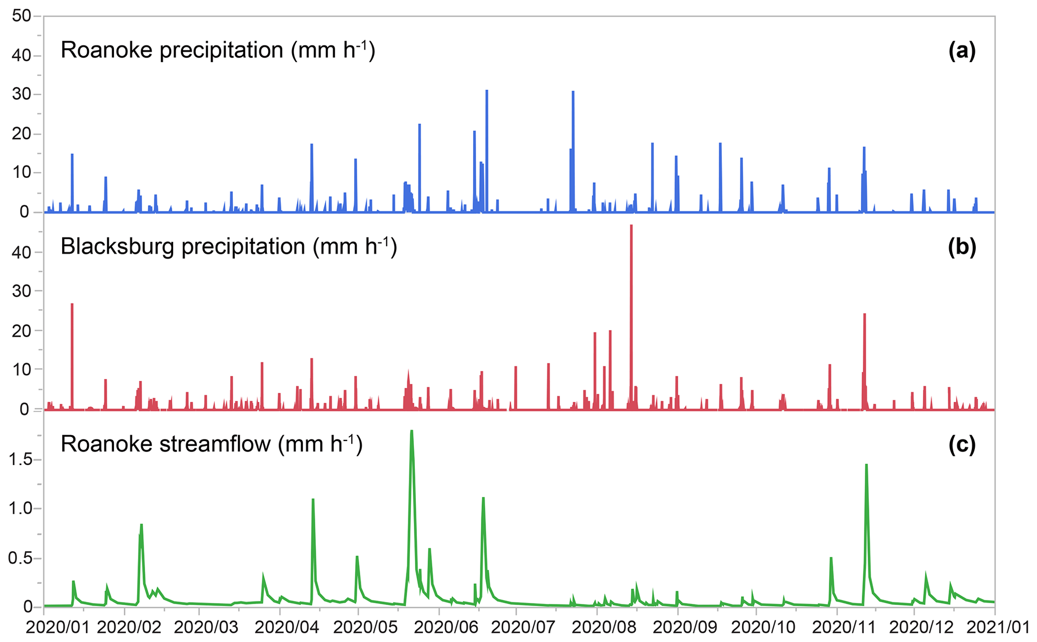
Figure 3 Hourly precipitation at the Roanoke and Blacksburg airports and hourly streamflow at the Roanoke gauge over 1 year. Note that the streamflow axis is expanded 25× relative to the precipitation axes.

2.2 Whole-catchment runoff response at Roanoke River

Here, I illustrate the estimation of runoff response distributions using the Roanoke River catchment, a 995 km² drainage basin with mixed land use lying between Blacksburg and Roanoke, Virginia, USA (Fig. 2). I extracted hourly precipitation time series for 2006–2022 from the aviation weather records at two airports located ∼ 40 km apart, just beyond the eastern and western catchment boundaries (Roanoke Regional Airport in Roanoke and Virginia Tech Montgomery Executive Airport in Blacksburg, respectively), and aggregated hourly streamflows for the same period from 15 min discharge data from USGS gauge 02055000 in downtown Roanoke (Fig. 2). Figure 3 shows 1 year of these hourly measurements. The Roanoke and Blacksburg precipitation time series are imperfectly correlated, with a Pearson correlation of 0.3 on an hourly timescale and of 0.7 on a daily timescale. Some precipitation events occur nearly simultaneously at both stations, but the Blacksburg time series contains some precipitation events that were not observed at Roanoke and vice versa, and events occurring at both locations often differ in magnitude or timing. From Fig. 3, one can also see that streamflow responds most strongly to precipitation that is recorded simultaneously, or nearly so, at both weather stations. This makes sense because such events are likely to have entailed widespread precipitation over most of the catchment.

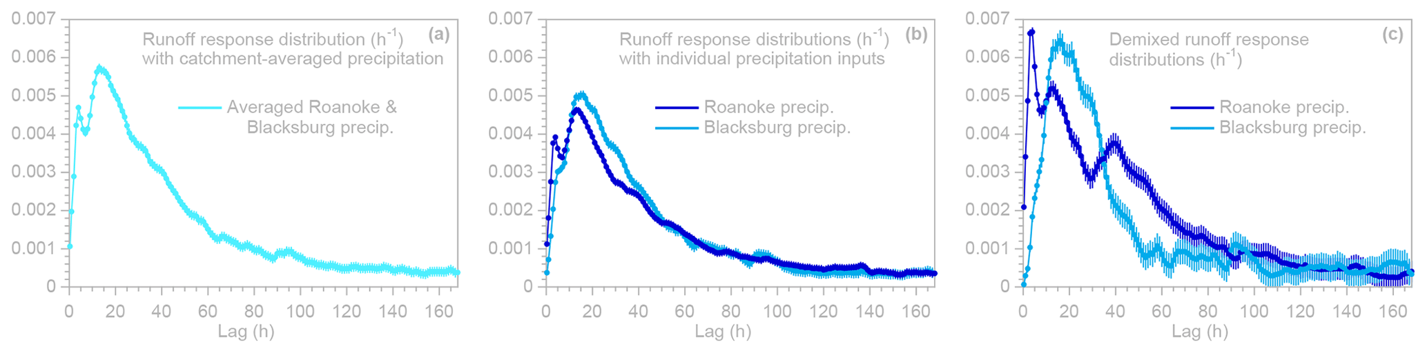
Figure 4 ERRA runoff response distributions calculated by deconvolving Roanoke River streamflow by different precipitation inputs. In (a), streamflow is deconvolved by the average of precipitation measured at Roanoke and Blacksburg using the approach outlined in Sect. 2.1. The same approach is used in (b) to deconvolve streamflow by either Roanoke precipitation alone (dark blue) or Blacksburg precipitation alone (light blue). In (c), by contrast, deconvolution and de-mixing are used to jointly determine the effects of Roanoke and Blacksburg precipitation on streamflow using the approach outlined in Sect. 2.3. This combined deconvolution and de-mixing analysis reveals that the effects of Roanoke and Blacksburg precipitation are markedly different. Error bars show 1 standard error.

In a typical catchment-scale analysis with multiple weather stations, the precipitation time series are usually averaged together to yield a single catchment-averaged input. Figure 4a shows the runoff response distribution (RRD) generated by using ERRA (Eq. 3, with ARMA noise correction as described in Sect. 2 of K2022) to deconvolve hourly Roanoke River streamflow by the average of Roanoke and Blacksburg hourly precipitation.

As the name implies, the RRD quantifies how the catchment's streamflow response is distributed over time per unit of precipitation. Because precipitation and streamflow are measured in the same units (mm h⁻¹), the RRD has dimensions of time⁻¹. If the catchment's response were linear and stationary (time-invariant), the RRD would be a complete description of its behavior; that is, convolving the precipitation time series with the RRD would yield the streamflow time series. In the more realistic case of a catchment that is approximately linear but nonstationary, the RRD approximates the ensemble average streamflow response to precipitation. If the catchment's runoff response scales nonlinearly with precipitation intensity, its average is best approximated by a precipitation-weighted average RRD, as described in Sect. 3.4 below.

The RRD shown in Fig. 4a shows that the peak streamflow response occurs approximately 15.4 ± 0.9 h after precipitation falls, but the streamflow response curve is broad, with a width at half-maximum of 39.2 ± 1.6 h. The integral under the curve yields an effective runoff coefficient of 0.286 ± 0.001 for all streamflow responses shorter than the maximum lag (here, 168 h = 1 week). When compared to the long-term ratio of 0.345 ± 0.005 between average streamflow (0.042 mm h⁻¹) and average precipitation (0.122 mm h⁻¹), this runoff coefficient implies that over 80 % of streamflow leaves the catchment within 1 week of the precipitation that triggered it, with longer-term baseflow comprising the remainder. Note that this should not be interpreted as “over 80 % of streamflow leaving the catchment within 1 week following the precipitation it originated from”, nor should the runoff coefficient of 0.289 be interpreted as “29 % of precipitation leaving the catchment as streamflow within 1 week”. Hydrometric data reflect the coupling between precipitation and streamflow but do not trace the movement of water itself. As noted in Sect. 1.1 above, decades of tracer data from many different catchments show that storm flow is often dominated by precipitation that fell weeks, months, or even years before and that has been stored within the catchment ever since.

A notable feature of Fig. 4a is the sharp spike in the runoff response distribution at a lag of roughly 4 h. Such a rapid and brief runoff response could potentially be generated by rain falling on the Roanoke metropolitan area and being routed rapidly over impermeable surfaces (denoted in red and purple in Fig. 2). One might attempt to gain some insight into this possibility by deconvolving streamflow by Roanoke precipitation alone and by comparing the resulting runoff response distribution (dark-blue curve in Fig. 4b) with one derived by deconvolving streamflow by Blacksburg precipitation alone (light-blue curve in Fig. 4b). This comparison appears to imply that Roanoke precipitation triggers a small additional short-term runoff response but that, otherwise, the runoff responses to Roanoke and Blacksburg precipitation are similar.

Such an interpretation would be naïve, however, because deconvolving streamflow by Roanoke precipitation does not measure the effects of precipitation falling on Roanoke alone. Instead, it measures the effects of any precipitation, falling anywhere in the catchment, that is correlated with the precipitation measured at Roanoke. In principle, of course, the ideal solution would be to obtain precipitation and streamflow measurements in subcatchments that isolate particular landscapes of interest, such as the Roanoke metropolitan area. But such subcatchment gauging data are unavailable in many situations like this one. How can we separate the effects of Roanoke and Blacksburg precipitation on streamflow if we only have streamflow measurements that integrate over the entire catchment?

2.3 Deconvolution and de-mixing of multiple precipitation inputs

The Roanoke and Blacksburg precipitation time series are correlated with one another, and their effects are not only convolved forward through time but are also mixed together at the catchment outlet. This is a common problem in rainfall–runoff analysis at the catchment scale: precipitation falling in different parts of the landscape with different hydrological properties may generate different streamflow responses, which may then be lagged and dispersed differently on their way to the basin outlet. Estimating the streamflow response to individual inputs therefore combines a deconvolution problem (one must un-scramble each input's temporally overlapping effects) and a de-mixing problem (one must separate the different inputs' effects from one another). As outlined in Sect. 3 of K2022, this combined deconvolution and de-mixing problem can be approached by analyzing the effects of the two precipitation inputs jointly as follows:

$$\begin{array}{}\text{(4)}& \begin{array}{rl}{Q}_j=& f_{\mathrm{A}}\sum _{k=\mathrm{0}}^m{\text{RRD}}_{\mathrm{A},k}{P}_{\mathrm{A},j-k}\mathrm{\Delta }t\\ & +f_{\mathrm{B}}\sum _{k=\mathrm{0}}^m{\text{RRD}}_{\mathrm{B},k}{P}_{\mathrm{B},j-k}\mathrm{\Delta }t,\end{array}\end{array}$$

where RRD_A and RRD_B are the runoff response distributions for precipitation inputs P_A and P_B, which are assumed to fall on fractions f_A and f_B of the catchment. Equation (4) can be re-cast as the multiple regression equation

$$\begin{array}{}\text{(5)}& Q_j=\sum _{k=\mathrm{0}}^m{\mathit{\beta }}_{\mathrm{A},k}{f}_{\mathrm{A}}{P}_{\mathrm{A},j-k}+{\mathit{\beta }}_{\mathrm{B},k}{f}_{\mathrm{B}}{P}_{\mathrm{B},j-k}+\mathit{\alpha }+{\mathit{\epsilon }}_j,\end{array}$$

which is identical to Eq. (3) and is solved identically, except for the fact that there are more coefficients to estimate (this approach could, of course, be generalized to any number of inputs as long as their time series are sufficiently distinct). Equation (5) is analogous to the “multiple-input single-output variable gain factor model” of Liang et al. (1994), although that approach was applied to flood routing, using the flows of tributaries rather than precipitation as inputs. The approach outlined in Eqs. (4) and (5) has been benchmark-tested using synthetic data in Sect. 3 of K2023; here, I show a simple application, for purposes of demonstration, using the Roanoke River basin. Readers should note that values of the runoff response distributions RRD_A and RRD_B will inevitably be inversely proportional to the mixing fractions f_A and f_B; there is no way to determine them independently without making additional assumptions. This is because a given precipitation input can generate (for example) twice the effect on runoff either by falling on twice as much of the catchment or by falling on a part of the catchment that is twice as responsive to precipitation. Therefore, although the shapes of the RRDs will be determined by the data, their absolute magnitudes will depend on the assumed values of f_A and f_B. Here, I assume that $f_{\mathrm{A}}=f_{\mathrm{B}}=\mathrm{0.5}$, which yields the RRDs shown in Fig. 4c.

As Fig. 4c shows, solving jointly for the effects of precipitation at Roanoke and Blacksburg reveals that they are markedly different, in sharp contrast to the results obtained in Fig. 4b by applying each precipitation record separately. Figure 4c reveals a sharp spike in the runoff response to Roanoke precipitation at a lag of just 3.9 ± 0.2 h (see the dark-blue curve in Fig. 4c), presumably reflecting the prevalence of impermeable surfaces in the metropolitan Roanoke area, as well as the relatively short network flow paths to the gauging station in downtown Roanoke. By contrast, there is almost no short-term runoff response at Roanoke that is attributable to Blacksburg precipitation (see the light-blue curve in Fig. 4c), presumably reflecting the lack of any short flow paths connecting precipitation falling near Blacksburg with the Roanoke gauging station. The peak runoff response to Blacksburg precipitation is delayed (17.5 ± 0.8 h) and relatively broad, presumably also reflecting the relative scarcity of impermeable surfaces within the catchment near Blacksburg (Fig. 2). The runoff response to Roanoke precipitation also shows a broad decline over lags ranging from about 15 to 60 h, presumably reflecting longer, slower flow paths to the gauging station, including via tributaries that flow westward before joining the main stream and flowing back eastward to Roanoke (see Fig. 2). A 50 / 50 mixture of the two response distributions shown in Fig. 4c almost exactly reproduces the response distribution to catchment-averaged precipitation shown in Fig. 4a. Thus, Fig. 4c implies that the short-term peak in the runoff response shown in Fig. 4a is generated by precipitation falling near Roanoke, and the broader, later peak is generated by precipitation falling near both Roanoke and Blacksburg.

These results have the practical implication that storms delivering the same catchment-averaged precipitation can yield very different hydrographs, depending on how much of that precipitation falls near Roanoke versus Blacksburg. Runoff responses to storms can also differ markedly, depending on whether they move from southwest to northeast (such that the runoff peaks from Blacksburg and Roanoke precipitation tend to coincide) or from northeast to southwest (increasing the separation between the arrival times of the runoff peaks at the outlet). More generally, the analysis presented here demonstrates that, whenever one has precipitation records for different parts of a catchment, one can quantify their individual effects on runoff even if the individual subcatchments are not separately gauged (as long as the subcatchments are not too numerous and their precipitation records are not too similar, which would be reflected in very large standard errors in the reported RRDs). In this way, one can explore how network routing and local variations in catchment characteristics affect runoff dynamics directly from data without positing a physical model and without subcatchment gauging data.

3 Quantifying nonlinearities and thresholds in runoff response via nonlinear deconvolution

3.1 Introduction: nonlinear deconvolution

It has long been recognized that storm runoff often responds more than proportionally to changes in precipitation intensity. For example, Fig. 5 shows unit hydrographs estimated for five brief (10–15 min) bursts of rainfall in an agricultural catchment in Illinois (data of Minshall, 1960). From Fig. 5, one can see that unit hydrograph peaks are both higher and earlier for higher-intensity storms in this small (11 ha) catchment. Conventional deconvolutions, and unit hydrographs in particular, are inconsistent with the behavior shown in Fig. 5 because they assume that outputs scale proportionally to inputs, leading Minshall (1960) to conclude that a single unit hydrograph cannot adequately characterize the runoff response to different precipitation intensities, at least in small catchments like those that he studied.

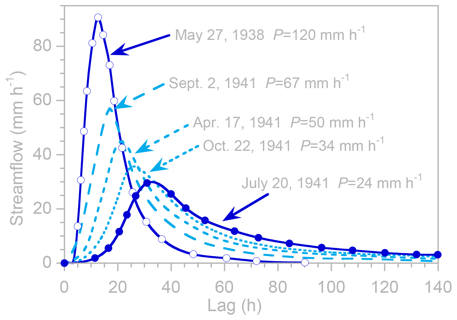
Figure 5 Unit hydrographs estimated by Minshall (1960) for 10–15 min periods of different rainfall intensities in an 11 ha catchment.

Here, I outline an approach to characterizing this type of nonlinear runoff response based on the nonlinear deconvolution method presented in Sect. 5 of K2022. The core of the problem is that one cannot directly observe a catchment's response to (for example) a single hour of precipitation at a given intensity because these responses are convolved forward through time, overlapping with the responses to other hours of precipitation at other intensities. To handle this problem, I adapt the methods outlined in Sect. 2 above by replacing each coefficient of the runoff response distribution with a function of the precipitation rate. If the RRD at each lag is a function of precipitation intensity, Eq. (2) becomes

$$\begin{array}{}\text{(6)}& Q_j=\sum _{k=\mathrm{0}}^m{P}_{j-k}{\text{RRD}}_k\left(P_{j-k}\right)\mathrm{\Delta }t,\end{array}$$

(see also Ding, 2011) where the parentheses indicate functional dependence rather than multiplication. Because rainfall is stochastic and its distribution is highly skewed, the precipitation intensity P_j−k will be inherently dependent on the duration Δt over which it is measured. The runoff response distribution RRD_k may, likewise, vary with the time step Δt. It may also be highly uncertain when precipitation intensity and the resulting runoff response are close to zero. For these reasons, and to more clearly visualize the functional relationship between precipitation intensity and streamflow response, it is useful to define a nonlinear response function NRF_k as the product between the precipitation-intensity-dependent RRD_k and the precipitation rate P:

$$\begin{array}{}\text{(7)}& {\text{NRF}}_k\left(P_{j-k}\right)=P_{j-k}{\text{RRD}}_k\left(P_{j-k}\right),\end{array}$$

where the parentheses indicate functional dependence rather than multiplication. Combining Eq. (7) and Eq. (6) yields

$$\begin{array}{}\text{(8)}& Q_j=\sum _{k=\mathrm{0}}^m{\text{NRF}}_k\left(P_{j-k}\right)\mathrm{\Delta }t,\end{array}$$

where Q_j is streamflow at time step j, P_j−k is precipitation occurring k time steps earlier, NRF_k is the nonlinear response of streamflow to precipitation that falls at a rate of P_j−k and lasts for a time step of Δt, m is the maximum lag being considered, and the parentheses indicate functional dependence rather than multiplication. From Eqs. (6) and (7), one can see that the units of the NRF will be millimeters per hour squared (mm h⁻²), consistent with its interpretation as the rate of streamflow expected to result at a given time lag k from precipitation falling at a rate P, per unit of time that this precipitation falls. In cases where the time step is equal to the time unit (for example, where precipitation and streamflow are measured in millimeters per hour (mm h⁻¹) over time steps of 1 h), the time step of Δt will equal 1, and the NRF will be numerically (though not dimensionally) equal to the increment of additional streamflow resulting from one time step of precipitation at rate P. Nonetheless, one can also consider the time step to be a part of the definition of the NRF (in this example, an “hourly” NRF) and can consider the NRF to be an estimate of the incremental addition to runoff (in mm h⁻¹) that would be expected to result from 1 h of precipitation at a given rate (or within a given range of rates). This alternative interpretation, in which the NRF has units of streamflow, will be more intuitive in many contexts, although the implicit timescale must be kept in mind.

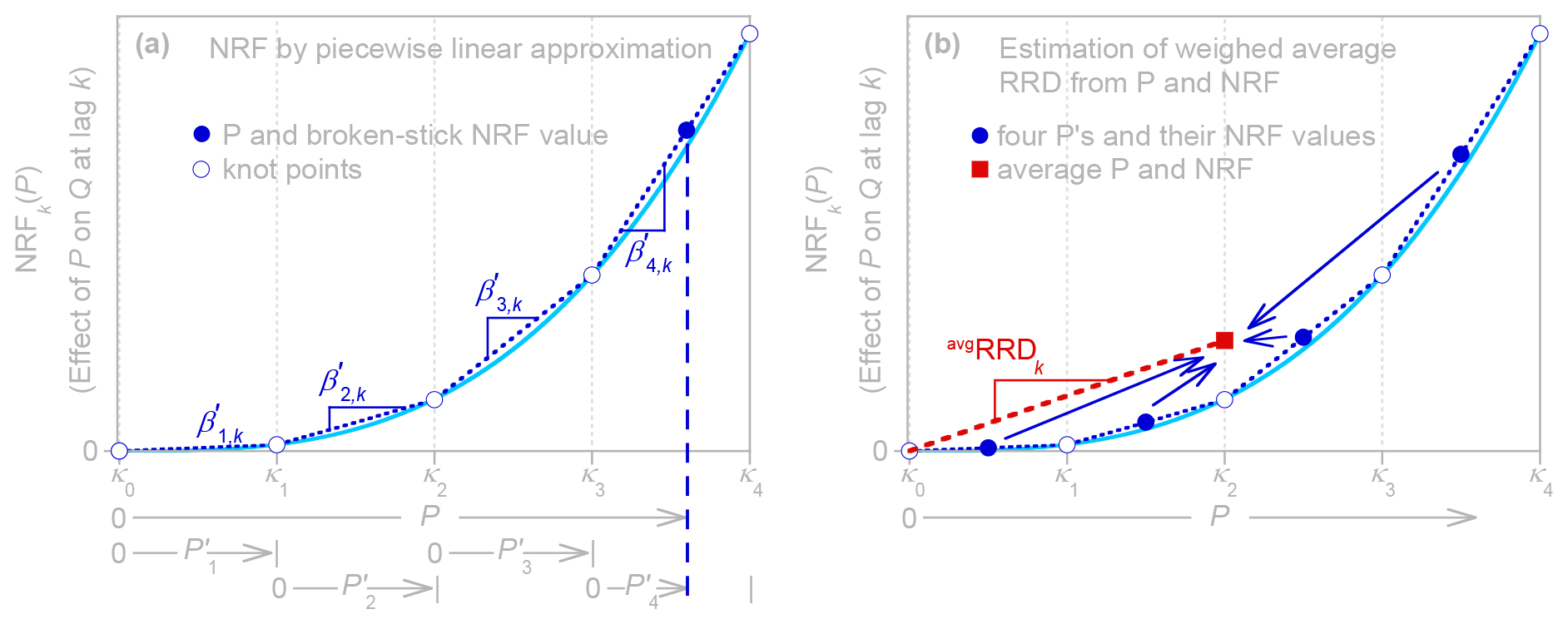
Figure 6 Nonlinear response function (NRF) estimation by piecewise-linear broken-stick approximation. (a) Estimation of the nonlinear dependence of Q on precipitation intensity P at a specified lag k. As described in Sect. 3.1, splitting the precipitation value P (solid circle) into sub-ranges $P_{\mathrm{\ell }}^{\prime }$ between user-specified knots κ_ℓ (open circles) facilitates the fitting of slopes ${\mathit{\beta }}_{\mathrm{\ell },k}^{\prime }$ between these knots by linear regression, yielding a nonparametric piecewise-linear continuous curve (see Eqs. 9 and 10). (b) Estimation of the weighted average runoff response distribution (RRD_k) as the ratio between the means of the NRF and P (red square) over all time steps (four example values of P and NRF shown by solid blue circles), as described in Sect. 3.4.

The question now becomes one of how to estimate the nonlinear response function NRF_k. We want to avoid needing to specify the form of this function and instead allow it to be determined from the data. The approach adopted here and in K2022, as illustrated schematically in Fig. 6a, is to approximate NRF_k using a continuous piecewise-linear broken-stick model, with linear segments intersecting at knots that correspond to user-defined precipitation intensities. Dividing the precipitation axis of Fig. 6 into n_κ segments between knots κ_ℓ allows precipitation intensity to be re-expressed as a vector of values $P_{\mathrm{\ell }}^{\prime }$ that quantify how much of each segment lies at or below any given value of P.

$$\begin{array}{}\text{(9)}& P=\sum _{\mathrm{\ell }=\mathrm{1}}^{n_{\mathit{\kappa }}}{P}_{\mathrm{\ell }}^{\prime },\begin{array}{l}{P}_{\mathrm{\ell }}^{\prime }=\left\{\begin{array}{ll}\mathrm{0}& \text{if }P<{\mathit{\kappa }}_{\mathrm{\ell }-\mathrm{1}}\\ P-{\mathit{\kappa }}_{\mathrm{\ell }-\mathrm{1}}& \text{if }{\mathit{\kappa }}_{\mathrm{\ell }-\mathrm{1}}\le P<{\mathit{\kappa }}_{\mathrm{\ell }}\\ {\mathit{\kappa }}_{\mathrm{\ell }}-{\mathit{\kappa }}_{\mathrm{\ell }-\mathrm{1}}& \text{if }P\ge {\mathit{\kappa }}_{\mathrm{\ell }}\end{array}\right.\\ =max(\mathrm{0},min(P-{\mathit{\kappa }}_{\mathrm{\ell }-\mathrm{1}},{\mathit{\kappa }}_{\mathrm{\ell }}-{\mathit{\kappa }}_{\mathrm{\ell }-\mathrm{1}}\left)\right)\end{array}\end{array}$$

The nonlinear response function NRF_k thus becomes the sum of these individual precipitation components, each multiplied by the slopes ${\mathit{\beta }}_{\mathrm{\ell },k}^{\prime }$ of the corresponding broken-stick segments (and rescaled by the time interval Δt):

$$\begin{array}{}\text{(10)}& {\text{NRF}}_k\left(P\right)\approx \sum _{\mathrm{\ell }=\mathrm{1}}^{n_{\mathit{\kappa }}}{\mathit{\beta }}_{\mathrm{\ell },k}^{\prime }{P}_{\mathrm{\ell }}^{\prime }/\mathrm{\Delta }t.\end{array}$$

The slopes ${\mathit{\beta }}_{\mathrm{\ell },k}^{\prime }$ can be estimated by a linear regression equation that is formed by combining Eqs. (10) and (8):

$$\begin{array}{}\text{(11)}& Q_j\approx \sum _{k=\mathrm{0}}^m\sum _{\mathrm{\ell }=\mathrm{1}}^{n_{\mathit{\kappa }}}{\mathit{\beta }}_{\mathrm{\ell },k}^{\prime }{P}_{\mathrm{\ell },j-k}^{\prime }+\mathit{\alpha }+{\mathit{\epsilon }}_j.\end{array}$$

For the methodological details underlying this approach, users are referred to Sect. 5 of K2022, and for practical implementation details, including different options for setting the knot values κ_ℓ, they are referred to the documentation for the ERRA script itself.

It is worth emphasizing that this approach differs from conventional transfer function models that use a nonlinear transformation to convert total rainfall to effective rainfall and then estimate a transfer function to route this rainfall through the catchment (e.g., IHACRES; Jakeman et al., 1990). The present approach, by contrast, estimates nonlinear relationships like those shown in Fig. 6 separately for each lag between 0 and m; in the conceptual framework of transfer function models, this means that the effective rainfall can vary with lag time.

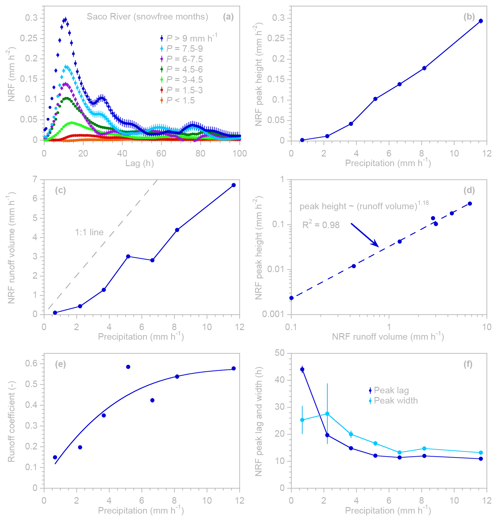
Figure 7 Nonlinear rainfall–runoff behavior at the Saco River near Conway, NH, USA, inferred from ERRA nonlinear response functions (NRFs). (a) NRF as a function of lag time for specified ranges of precipitation intensity. (b) Peak height of NRFs as a function of precipitation intensity, showing nonlinearity in peak runoff response. (c) Effect of precipitation intensity on NRF runoff volume, measured as the total area under each curve in panel (a) and expressed in millimeters of streamflow per hour of precipitation at the stated intensity. Runoff volume increases more slowly than precipitation intensity does (i.e., the gap between the blue curve and the gray 1:1 line continues to grow), suggesting that losses to evapotranspiration and/or long-term storage are not constant but instead increase with increasing precipitation intensity. (d) Log–log relationship between NRF peak height and NRF runoff volume, with a scaling exponent of 1.16, indicating that peak height is modestly more sensitive to precipitation intensity than total runoff volume is. Thus, as precipitation intensity increases, peak height grows more than proportionally relative to average runoff response. (e) Runoff coefficient (ratio between NRF runoff volume and precipitation intensity) as a function of precipitation intensity, with an arbitrary smooth curve to guide the eye. (f) Lag to peak and peak width (at half maximum) as functions of precipitation intensity, showing that NRF peaks are earlier and narrower at higher precipitation rates. Source data span 1987–2003; months from November through April were omitted to exclude effects of snow. Error bars show 1 standard error, where this is larger than the plotting symbols.

3.2 Profiles of nonlinear response at the Saco River

Figure 7 illustrates the approach outlined above, using the Saco River as a test case. At the Conway, NH, stream gauge, the Saco River drains 997 km² of the White Mountains. I aggregated USGS 15 min discharge measurements from the Conway gauge to hourly intervals to correspond with hourly estimates of catchment-averaged precipitation that are available from MOPEX (Duan et al., 2006). To minimize the effects of snow, the months of November through April were excluded. In all, about 16 years of overlapping hourly precipitation and discharge data are available, spanning 1987 through 2003.

Figure 7a shows NRF estimates of the Saco River's runoff response to seven ranges of precipitation intensity, as estimated by Eq. (11). Unsurprisingly, the highest precipitation intensities yield the strongest runoff responses and the highest peaks. They also have the largest error bars because the precipitation distribution is highly skewed, and, thus, the highest intensity ranges contain relatively few data points. The peak height, calculated from a quadratic fit to all NRF values within 20 % of the peak, increases nonlinearly with precipitation intensity, presumably reflecting the effects of interception losses and of refilling of near-surface storage (Fig. 7b).

The total runoff volume, calculated by integrating the NRF over the 100 h range of lag times shown in Fig. 7a, also increases nonlinearly with precipitation intensity (Fig. 7c). Because the units of the NRF are millimeters per hour squared (mm h⁻²), the units of the runoff volume shown in Fig. 7c are millimeters per hour (mm h⁻¹), which is millimeters of streamflow (here, in the first 100 h following precipitation) per hour of precipitation at a given intensity or over a given intensity range. One could also equivalently consider Fig. 7c to be a plot of 1 h precipitation intensity in millimeters (on the x axis) versus the total streamflow resulting from 1 h of that precipitation within the first 100 h (on the y axis). The gap between the runoff volume curve and the 1:1 line in Fig. 7c indicates the volume lost to interception and evapotranspiration, as well as to infiltration that does not generate streamflow within 100 h.

Peak height increases with runoff volume following a power function with an exponent greater than 1 (Fig. 7d). This more-than-proportional increase in peak height implies that higher precipitation intensities do not amplify runoff response by the same proportion at all lags but instead amplify runoff response near the peak lag by somewhat larger factors. The runoff coefficient, calculated as the ratio between the y and x axes of Fig. 7c, increases with precipitation intensity, reflecting the greater relative importance of interception losses and storage deficits at lower precipitation rates (Fig. 7e). The runoff coefficient appears to reach an upper limit of approximately 0.6, suggesting that, even at high precipitation rates, interception and infiltration losses may remain significant. Runoff response peaks are narrower and earlier at higher precipitation rates (Fig. 7f). Figure 7b–f can be considered to be profiles of nonlinear hydrological response and, thus, fingerprints of catchment behavior. Controls on nonlinear hydrological response may potentially be illuminated by comparing these response profiles among streams with different catchment characteristics.

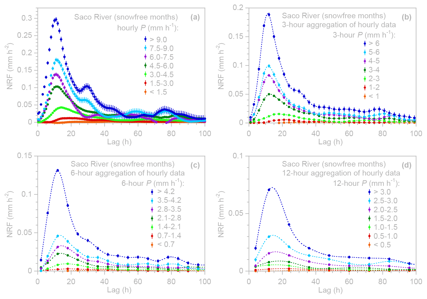
Figure 8 Effects of time step aggregation on inferred nonlinear runoff response of the Saco River. Panels (a–d) show ERRA nonlinear response functions (NRFs) as functions of lag time for specified ranges of precipitation intensity using hourly precipitation and streamflow time series (a) and the same data aggregated by averaging over 3 h (b), 6 h (c), and 12 h (d). Average precipitation intensity is lower and runoff responses are correspondingly more muted when precipitation and discharge are averaged over longer spans of time. Source data span 1987–2003; months from November through April were omitted to exclude any effects of snow. Error bars show 1 standard error.

3.3 Effects of sampling interval on nonlinear response functions

The stochastic nature of precipitation means that precipitation rates measured over different time intervals will have different distributions. This naturally leads to the question of how the results reported in Fig. 7 might look different if precipitation rates and runoff responses were measured at different time resolutions.

This question is important because one may want to compare runoff responses at different catchments that have different sampling frequencies. Furthermore, when the sampling interval is much shorter than the response time of the catchment itself, the runoff time series will be strongly autocorrelated and so will the residuals of analyses such as Eqs. (3), (5), or (11). ERRA is designed to handle autocorrelated residuals, but if the autocorrelation is too strong (e.g., lag−1 residual autocorrelation > 0.99), the NRF and RRD may exhibit spurious features. These problems can generally be avoided by aggregating the input data over longer and longer time steps until the residual autocorrelation becomes manageable. Thus, it is important to understand how aggregating the underlying time series might affect the results obtained from ERRA.

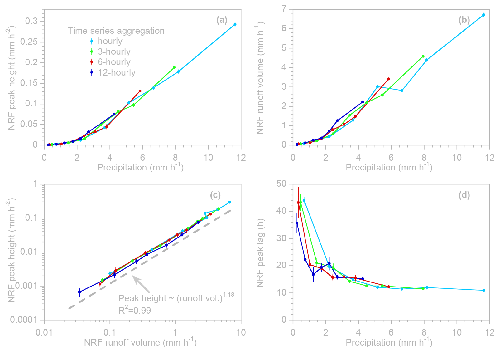
Figure 9 Nonlinear responses of peak heights, peak lags, and runoff volumes to variations in precipitation intensity at the Saco River, estimated from precipitation and streamflow data aggregated over different time intervals. Time step aggregation reduces average precipitation intensity and damps the resulting nonlinear response functions (NRFs; Fig. 8). However, the nonlinear response curves relating peak heights (a) and runoff volumes (b) to precipitation intensity plot on top of one another at different levels of time step aggregation, as do the power-law relationships between peak heights and runoff volumes (c) (dashed gray line is offset from the data for clarity). Time step aggregation has little effect on lag-to-peak (d) at high precipitation intensities but may have a more noticeable effect at low precipitation intensities. Source data span 1987–2003; months from November through April were omitted to exclude any effects of snow. Error bars show 1 standard error.

Figure 8 shows the runoff response curves for the Saco River, with precipitation and streamflow aggregated over intervals from 1 to 12 h. The timing of the peak response and the shapes of the curves are similar across the different timescales, but the precipitation intensities – and, thus, the NRF values – decrease with increasing time aggregation. However, as Fig. 9 shows, the underlying relationships between runoff response peak height, runoff volume, peak lag, and precipitation intensity are generally consistent across the different measurement intervals, with each of the response profiles lying approximately on top of one another. Longer aggregation timescales, however, inherently lead to smaller ranges of precipitation intensities, with the result being that a smaller part of the response profile is visible. Thus, the results obtained from ERRA at different levels of time step aggregation are consistent with one another but are not equivalent to one another.

3.4 Average of nonlinear runoff response

The NRF quantifies the system's ensemble-averaged response to time steps of rain falling at an intensity of P (averaged over the time step). The NRF is not, however, normalized by precipitation intensity like the RRD is. For any individual value of P, one could straightforwardly estimate the runoff response per unit of precipitation as ${\text{NRF}}_k\left(P\right)/P$. This could be viewed as the runoff response distribution for a specific precipitation intensity, as in Eq. (6), but one should be aware that it may yield highly uncertain results for low-intensity precipitation with a small runoff response. A better approach, and the one adopted in ERRA, is to define the weighted average runoff response distribution as equalling the average of the NRF over all time steps, divided by the average P, as illustrated schematically in Fig. 6b. This will equal the precipitation-weighted average of the runoff response distribution RRD_k(P_j−k) over all time steps.

$$\begin{array}{}\text{(12)}& \begin{array}{rl}{}^{\text{avg}}{\text{RRD}}_k& ={\displaystyle \frac{\sum _{j=\mathrm{1}}^{n-k}{\text{NRF}}_k\left(P_{j-k}\right)}{\sum _{j=\mathrm{1}}^{n-k}{P}_{j-k}}}\mathrm{\Delta }t\\ & ={\displaystyle \frac{\sum _{j=\mathrm{1}}^{n-k}{P}_{j-k}{\text{RRD}}_k\left(P_{j-k}\right)}{\sum _{j=\mathrm{1}}^{n-k}{P}_{j-k}}}\end{array}\end{array}$$

This average runoff response distribution will be inherently dependent on the distribution of precipitation intensities whenever the system response is nonlinear. Readers should also note that, whenever the runoff response is nonlinear and, thus, the underlying relationship between NRF and P is curved, the point defining the average P and average NRF (e.g., the red square in Fig. 6b) will not lie along the function NRF(P) but instead will lie inside of the curve. Thus, in the typical case of an upward-curving NRF, the average NRF will be greater than the value of the NRF evaluated at the average P; thus, the weighted average RRD will also be greater than the RRD evaluated at the average P. The weighted average RRD is nonetheless the average runoff response per unit of precipitation (averaged over the nonlinear relationship between precipitation intensity and runoff response) and, thus, is the closest analogue to the runoff response distribution of a linear system.

One should also be aware that, if the system's response is nonlinear, RRD values calculated via Eqs. (1)–(3) – that is, without recognition of the system's nonlinearity – will generally overestimate the precipitation-weighted average RRD (Eq. 12). This overestimation bias arises because precipitation distributions typically have very long upper tails, and so the highest precipitation points (whose leverage scales as roughly P²) have a disproportionate influence on the RRD estimate. This bias, which is inherent in all regression-based estimates of unit hydrographs, may be desirable if one wants an estimate that is skewed toward the catchment response to high-intensity precipitation. However, if one wants to capture the average of the nonlinear runoff response, the approach outlined in Eqs. (6)–(12) will be needed.

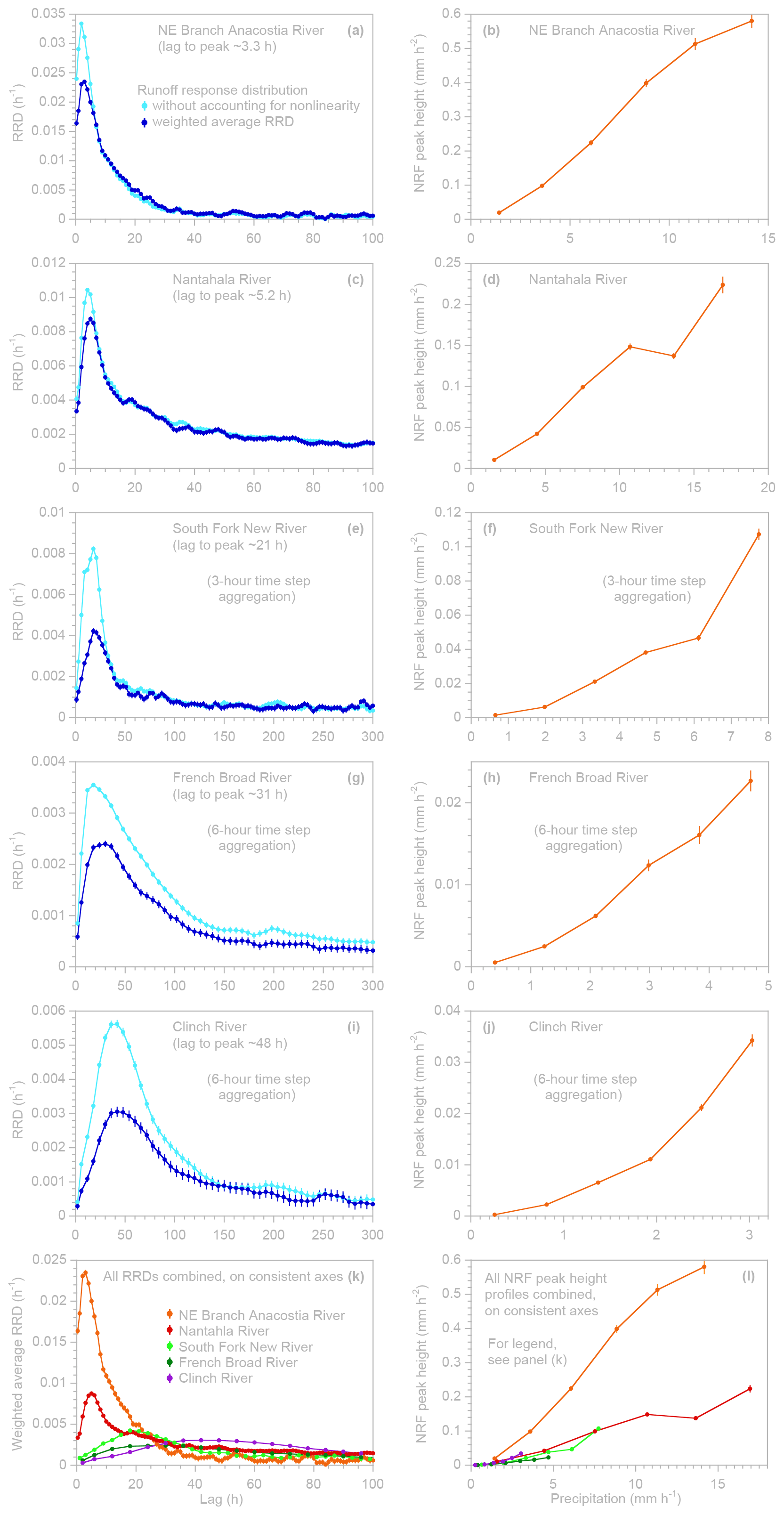
Figure 10 Runoff response distributions (RRDs) calculated with (dark blue) and without (light blue) accounting for nonlinear response to precipitation intensity (left panels) and profiles of nonlinear response function (NRF) peak height as a function of precipitation intensity (right panels) for five mesoscale river basins in the southeastern US. Basins are the Northeast Branch of the Anacostia River at Riverdale, MD (a, b: 189 km²); the Nantahala River near Rainbow Springs, NC (c, d: 134 km²); the South Fork New River near Jefferson, NC (e, f: 531 km²); the French Broad River at Asheville, NC (g, h: 2448 km²); and the Clinch River above Tazewell, TN (i, j: 3818 km²). Weighted average RRDs, calculated via Eq. (12) to take account of nonlinear responses (dark blue, left panels), are less strongly peaked and peak a bit later than RRDs calculated without taking nonlinearity into account (light blue, left panels). Note that the axis scales differ substantially among the different panels. All sites' weighted average RRDs and NRF peak height profiles are shown on consistent axes in panels (k) and (l). At several sites with delayed and long-lasting runoff response, time steps were aggregated to 3 or 6 h to prevent the residual autocorrelation from becoming excessive. Error bars indicate 1 standard error.

Here, I illustrate this approach using rainfall–runoff data from five rivers in the southeastern US that exhibit different degrees of nonlinearity and markedly different response times (Fig. 10). As in Sect. 3.2 above, I aggregated 15 min discharge measurements from USGS gauges on each of these rivers to hourly intervals and combined them with hourly estimates of catchment-averaged precipitation that are available from MOPEX (Duan et al., 2006) for the corresponding drainage basins. The resulting time series for the five sites span between 13 and 18 years of hourly data.

As Fig. 10 shows, precipitation-weighted average RRDs calculated via Eq. (12) for all five sites are less strongly peaked (dark-blue symbols, left panels) than unweighted RRDs (light-blue symbols, left panels) calculated via Eqs. (1)–(3). It may seem counterintuitive that the unweighted RRDs are more strongly peaked and that accounting for the nonlinearities in runoff response and weighting by precipitation dampens the RRD peaks rather than sharpening them. But it is important to remember that, as noted above, because the mean P is close to zero, each point's leverage in Eq. (3) is approximately P²; thus, the “unweighted” RRDs are implicitly weighted by the square of precipitation. The resulting overestimation bias is greatest at sites like the Clinch River or the South Fork New River, where the NRF peak is a strongly nonlinear function of precipitation intensity. By quantifying this nonlinearity and explicitly weighting by P, the approach of Eqs. (9)–(12) corrects the overestimation bias that arises in simpler approaches like Eqs. (1)–(3) and in similar regression-based approaches to unit hydrograph estimation.

Figure 10 also demonstrates a wide range of hydrologic response timescales among the five catchments, with the peak runoff response in the weighted average RRD ranging from just over 3 h (for the Northeast Branch of the Anacostia River at Riverdale, Maryland, draining 189 km² of a mostly suburban landscape north of Washington DC) to 48 h (for the Clinch River above Tazewell, Tennessee, draining 3818 km² of mostly forests and farmlands of the Appalachian Mountains). Notably, only the slowest runoff responses among these sites would be captured by daily time series, which are widely used for hydrological analysis and modeling. Thus, daily time series and models that are calibrated to them may fail to reflect the rapid dynamics that characterize runoff response in many landscapes.

3.5 Nonlinear storage–discharge relationships

It should be clear that, here, in Sect. 3, the term “nonlinear” refers to catchments that respond nonlinearly to variations in precipitation intensity, as shown, for example, in Figs. 7–9. Elsewhere in the hydrological literature, the term “nonlinear” has also been used to refer to catchments in which streamflow is a nonlinear function of catchment storage:

$$\begin{array}{}\text{(13)}& Q=f\left(S\right),{\displaystyle \frac{\mathrm{d}S}{\mathrm{d}t}}=P-E-Q,\end{array}$$

where Q, S, P, and E (discharge, storage, precipitation, and evapotranspiration, respectively) are all functions of time, and the function f may have any general nonlinear form. Data-driven streamflow prediction models for such systems can be fitted using Volterra series (e.g., Amorocho, 1967; Kothyari and Singh, 1999), which represent streamflow as a linear function of a multidimensional array of past inputs. But even a second-order Volterra series requires $m\cdot (\mathrm{1}+\frac{m+\mathrm{1}}{\mathrm{2}})$ coefficients, and a third-order series requires $m\cdot (\mathrm{1}+\frac{m+\mathrm{1}}{\mathrm{2}}\cdot (\mathrm{1}+\frac{m+\mathrm{2}}{\mathrm{3}}\left)\right)$ coefficients, where m is the number of lags, such that the coefficients can rapidly become too numerous to estimate accurately. This overfitting problem can be handled using regularization methods (Kothyari and Singh, 1999) or by approximating the (multidimensional) response function with polynomials such as Meixner functions or Chebyshev polynomials (Amorocho and Brandstetter, 1971), which can greatly reduce the number of coefficients to be estimated at the cost of obscuring sharp features in the response function. Whatever the specific calculation procedure, however, a Volterra series is difficult to interpret in terms of impulse response (i.e., a runoff response distribution).

As illustrated in Fig. 1, the runoff response of a nonlinear system such as Eq. (13) to individual precipitation inputs will depend on both past rainfall (which determines antecedent moisture) and future rainfall (which amplifies the runoff response of a given storm). Thus, the NRF should not be expected to accurately reflect the catchment's response to each individual precipitation event, which is in contrast to linear systems (for which the RRD should completely describe every event's runoff response). However, as Fig. 1e illustrates, even though a nonlinear system's responses to individual rain events may be highly variable, an ensemble of such events can yield reliable estimates of the NRF and weighted average RRD because it averages over the confounding effects of past and future inputs.

From the impulse response perspective that is the focus of this paper, a nonlinear system such as Eq. (13) is more properly considered to be both nonlinear and nonstationary because, even if the coefficients of the function f are constant over time, the response to precipitation will depend not only on input intensity but also on the value of the storage S (and thus on the prior history of inputs, which is what the Volterra series aims to capture). The next section presents methods for quantifying how antecedent wetness and other nonstationary catchment properties affect runoff response to precipitation.

4 Quantifying nonstationary controls on runoff response

4.1 Introduction

From the impulse response perspective, a catchment's wetness status is a nonstationary property that influences its response to precipitation falling at any moment. Other examples of nonstationary properties influencing runoff response include air temperature (which influences the phase of precipitation and the energy available to drive evapotranspiration), vapor pressure deficit (which influences how rapidly intercepted precipitation evaporates), and the leaf area index of vegetation (which influences how much precipitation is intercepted in the first place). Thus, the same precipitation inputs may generate substantially different runoff responses, depending on the ambient conditions. Precipitation inputs themselves may also change those ambient conditions (for example, by increasing soil moisture and reducing the vapor pressure deficit) and, thus, may influence catchment response to future precipitation inputs.

The challenge, then, is to characterize how a landscape's response to precipitation inputs will vary, depending on the ambient conditions when those inputs fall. This is both a deconvolution problem (because the lagged effects of precipitation inputs are overprinted on each other) and a de-mixing problem (because the effects of precipitation falling under one set of ambient conditions are overprinted on the effects of precipitation falling at other times under other ambient conditions). These two problems can be solved simultaneously via a combined deconvolution and de-mixing approach analogous to that presented in Sect. 2.3 above. In a simple case, we might be able to separate the precipitation time steps into two groups according to the ambient conditions when the rain falls (for example, groups A and B corresponding to antecedent wetness above and below a particular value). Then, if we use RRD_A,k and RRD_B,k to represent the runoff response distributions over lags k resulting from precipitation that falls under wet and dry antecedent conditions, respectively, the discharge time series becomes

$$\begin{array}{}\text{(14)}& Q_j=\sum _{k=\mathrm{0}}^m{\text{RRD}}_{\mathrm{A},k}{P}_{\mathrm{A},j-k}\mathrm{\Delta }t+\sum _{k=\mathrm{0}}^m{\text{RRD}}_{\mathrm{B},k}{P}_{\mathrm{B},j-k}\mathrm{\Delta }t,\end{array}$$

where Q_j is streamflow at time step j, $P_{\mathrm{A},j-k}$ is precipitation falling k time steps earlier under wet conditions (and zero otherwise), and $P_{\mathrm{B},j-k}$ is precipitation falling k time steps earlier under dry conditions (and zero otherwise). Equation (14) can be re-cast as the multiple regression equation

$$\begin{array}{}\text{(15)}& Q_j=\sum _{k=\mathrm{0}}^m{\mathit{\beta }}_{\mathrm{A},k}{P}_{\mathrm{A},j-k}+{\mathit{\beta }}_{\mathrm{B},k}{P}_{\mathrm{B},j-k}+\mathit{\alpha }+{\mathit{\epsilon }}_j,\end{array}$$

which is identical to Eq. (5), except it lacks the area fractions f_A and f_B. Section 4 of K2022 outlines the derivation of this approach and presents several benchmark tests of it. This approach can be combined with the nonlinear deconvolution methods outlined in Sect. 3 above, yielding regression equations of the form

$$\begin{array}{}\text{(16)}& Q_j\approx \sum _{k=\mathrm{0}}^m\sum _{\mathrm{\ell }=\mathrm{1}}^{n_{\mathit{\kappa }}}{\mathit{\beta }}_{\mathrm{A},\mathrm{\ell },k}^{\prime }{P}_{\mathrm{A},\mathrm{\ell },j-k}^{\prime }+{\mathit{\beta }}_{\mathrm{B},\mathrm{\ell },k}^{\prime }{P}_{\mathrm{B},\mathrm{\ell },j-k}^{\prime }+\mathit{\alpha }+{\mathit{\epsilon }}_j,\end{array}$$

which quantify the combined effects of variations in antecedent wetness and precipitation intensity. It should be clear that Eqs. (14)–(16) can be generalized to any number of categories, potentially representing combinations of different ambient conditions (such as, for example, multiple levels of antecedent wetness in both the growing season and the dormant season). It should also be clear that these categories can include time itself to test whether runoff response is nonstationary over time (between decades, between seasons, or between day and night, for example), even if the factors responsible for that nonstationary behavior are unknown.

ERRA can automatically separate the precipitation time series according to defined ranges (expressed as either values or percentiles) of nested combinations of multiple variables and can quantify the runoff response across all of these categories simultaneously while also correcting for ARMA noise (as outlined in Sect. 2 above and described in more detail in Sect. 2 of K2022).

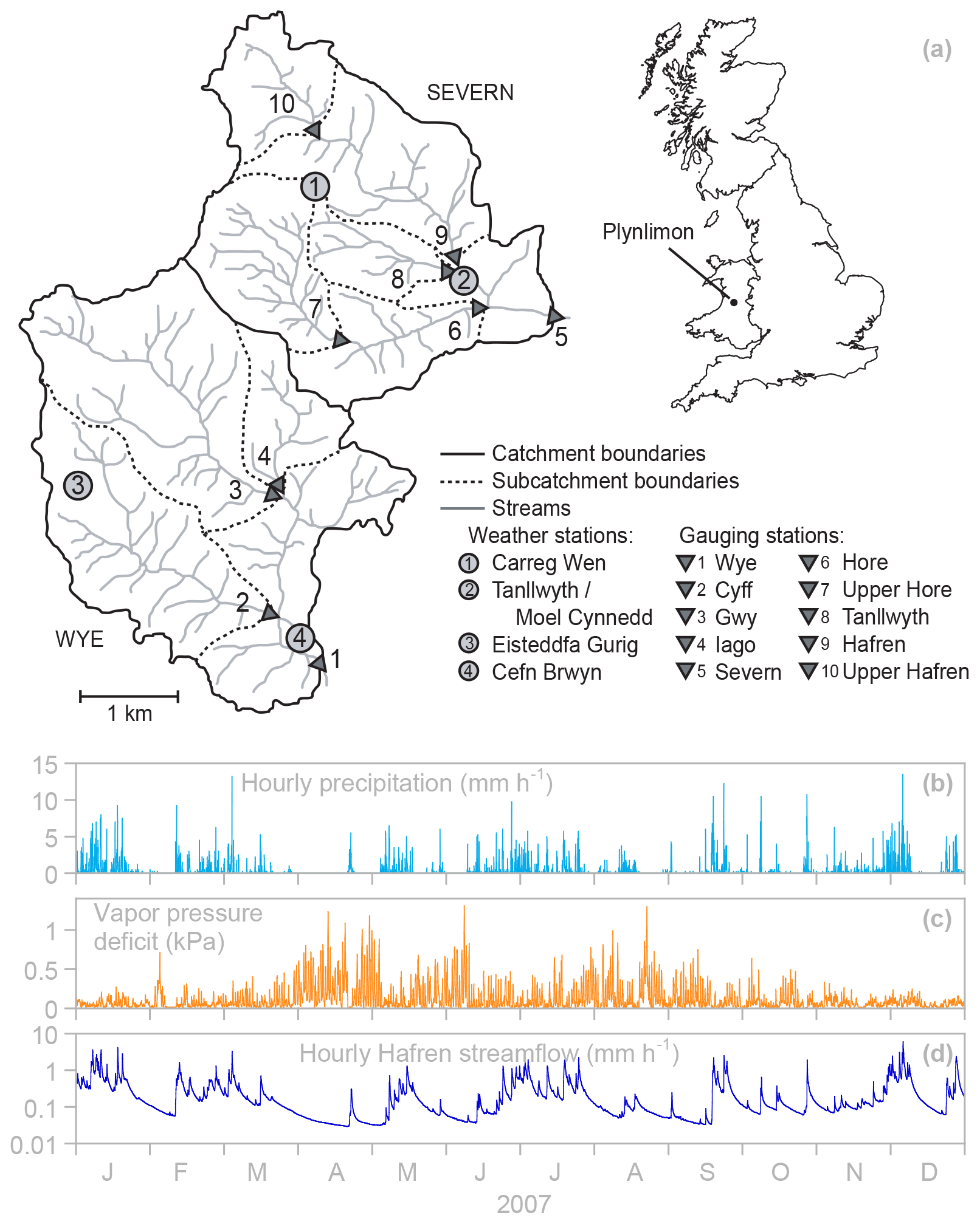
Figure 11 Map of the Plynlimon research catchments (a), redrawn with permission from Kirchner (2009), and one example year of hourly time series of precipitation (b), vapor pressure deficit (c), and Hafren streamflow (d). Permission for the re-use and/or modification of this figure can be found at the following link: https://www.agu.org/publish-with-agu/publish/agu-publications-policies (last access: 7 August 2024).

4.2 Proof of concept

Here, I illustrate this approach using rainfall–runoff data from the Plynlimon research catchments in Wales (Fig. 11). Hourly weather data are available from four weather stations, and discharge data are available every 15 min from 10 stream gauges with drainage areas ranging from 0.9 to 10.5 km². For seven of these gauges, records are available for at least 35 years from the mid-1970s through 2010 (Marc and Robinson, 2007); more recent measurements are also available, but here I analyze older data that have been extensively quality-controlled. The climate is generally cool and humid, with annual precipitation averaging roughly 2500–2600 mm yr⁻¹ (Marc and Robinson, 2007); over 70 % of days have some measurable precipitation, and over 24 % of days have precipitation totals exceeding 10 mm. The resulting hydrographs are flashy, with many high-flow events each year (Fig. 11b–d).

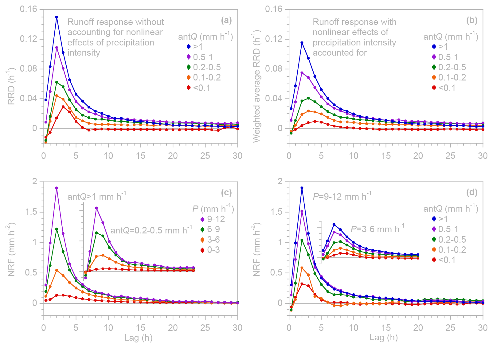
Figure 12 Runoff responses at Hafren, estimated via Eq. (16) as functions of precipitation intensity P and antecedent wetness (using 1 h antecedent discharge, antQ, as a proxy). (a) Runoff response distributions (RRDs) for different ranges of antQ, calculated using Eq. (15) without accounting for nonlinear effects of P or co-variation between P and antQ. Peak runoff response is somewhat exaggerated due to the greater leverage of high precipitation values (see text). (b) Precipitation-weighted average RRDs for different ranges of antQ, with nonlinear effects of P and co-variation between P and antQ taken into account via Eq. (15). Peak runoff responses in weighted average RRDs (b) are less pronounced relative to unweighted RRDs (a), particularly under drier antecedent conditions. (c) Effects of variations in precipitation intensity P (shown by different colors) for two example ranges of antQ (as a proxy for antecedent wetness), illustrating how runoff response under drier antecedent conditions (lower antQ: inset figure) is less pronounced across all ranges of precipitation intensity. (d) Effects of variations in antQ (shown by different colors, as a proxy for antecedent wetness) for two example ranges of precipitation intensity P, illustrating how runoff response to lower-intensity precipitation (lower P: inset figure) is less pronounced across all ranges of antQ. Insets in (c) and (d) are on the same axis scales as the main figures but are cropped and offset for compact presentation. Error bars indicate 1 standard error, where this is larger than the plotting symbols.

Using hourly data from 1976 to 2010 for the 3.6 km² Hafren catchment as a proof-of-concept case (catchment 9 in Fig. 11a, with precipitation estimated by averaging measurements at weather stations 1 and 2 in Fig. 11a), I tested how runoff responses to precipitation vary between wet and dry antecedent conditions (Fig. 12). Because long-term records of soil moisture or groundwater levels are not available, I use antecedent discharge (antQ, the streamflow measured during the hour before rain falls) as a proxy for antecedent wetness at the catchment scale (this may be a less effective proxy in large catchments with long lag times). Figure 12a shows RRDs estimated via Eq. (15) for five ranges of antecedent discharge, separated by the approximate 40th, 67th, 90th, and 97th percentiles of the Hafren discharge distribution. For the same five ranges of antecedent discharge, Fig. 12b shows weighted average RRDs, estimated via Eq. (12) from nonlinear response functions that account for nonlinear effects of variations in precipitation intensity.

The runoff response shown in Fig. 12a and b is markedly larger, and somewhat quicker, under wetter antecedent conditions. Readers may worry that this is an artifact of the use of antecedent discharge as a measure of antecedent wetness. However, the RRDs in Fig. 12 are not determined by discharge itself (which would, indeed, be correlated with antecedent discharge) but rather by how much discharge changes, depending on how much precipitation falls (see Eqs. 3 and 15). Thus, the effects of antecedent discharge on the RRDs are not artifactual.

One would expect that runoff response under a given antecedent wetness condition may depend on precipitation intensity and, likewise, that runoff response for a given precipitation intensity may depend on antecedent wetness. Figure 12c and d illustrate the combined effects of antecedent wetness and precipitation intensity on runoff response at Hafren. Figure 12c shows how the NRF varies with precipitation intensity (shown by the different colors) for two different ranges of antecedent wetness (shown by the main plot for high antQ and by the inset plot for moderate antQ). Similarly, Fig. 12d shows how the NRF varies with antecedent wetness (shown by the different colors) for two different ranges of precipitation intensity (9–12 mm h⁻¹, shown in the main plot, and 3–6 mm h⁻¹, shown in the inset plot). Both Fig. 12c and d demonstrate that the shape, scale, and timing of runoff response can depend jointly on both antecedent wetness and precipitation intensity. For example, 1 h of precipitation at an intensity of 9–12 mm h⁻¹ can be expected to raise stream discharge by a maximum of ∼ 2 mm h⁻¹ at a lag of ∼ 2 h if it falls under high-antecedent-wetness conditions (purple curve in the main plot in Fig. 12c or blue curve in the main plot in Fig. 12d) but only by ∼ 1 mm h⁻¹ if it falls under moderate-antecedent-wetness conditions (purple curve in the inset plot in Fig. 12c or green curve in the main plot in Fig. 12d). In other words, Fig. 12c and d reveal a runoff response that is nonstationary (i.e., dependent on the antecedent wetness in the landscape when rain falls) and that also scales nonlinearly with precipitation intensity.

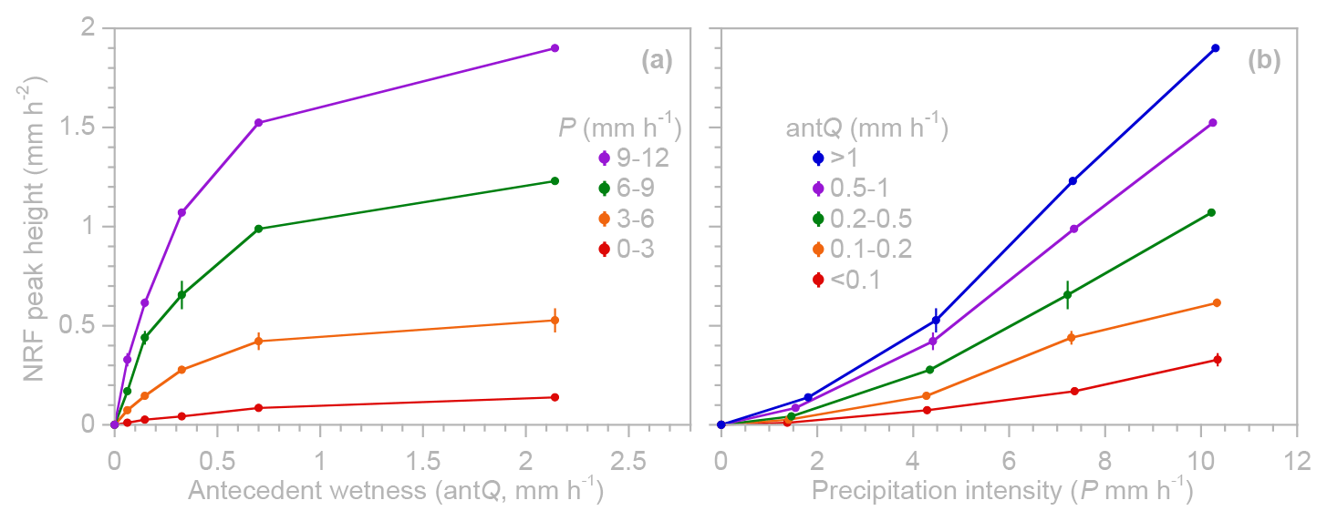
Figure 13 Peak runoff response at Hafren as a joint function of precipitation intensity P and antecedent wetness (using 1 h antecedent discharge, antQ, as a proxy). (a) Peak height of the nonlinear response function (NRF) as a function of antecedent wetness for four ranges of precipitation intensity (shown by different colors). (b) Peak height as a function of precipitation intensity for five ranges of antecedent wetness (shown by different colors). Error bars indicate 1 standard error, where this is larger than the plotting symbols.

Readers will notice that several of the RRD and NRF values in Fig. 12 are below zero. ERRA does not artificially constrain NRF and RRD coefficients to be non-negative, so small negative values may occur from time to time for at least three reasons. The first is random statistical fluctuations: if the true value of a coefficient is positive but small then random noise may lead to stochastic fluctuations in the coefficient estimates that occasionally dip below zero. In this case, one would usually expect the error bars to be roughly as large as the deviation below zero. This is not the case in Fig. 12, where the error bars are almost always smaller than the plotting symbols. A second reason for negative values can be residual autocorrelation that is too strong to be adequately compensated for by the ARMA noise correction procedure, which can lead to spurious patterns in the NRF or RRD coefficients and to underestimation of the error bars (for this reason, ERRA issues warnings when it detects strong residual autocorrelation). A third reason can be confounding variables that are not included in the analysis and whose effects are aliased as distortions of the NRF or RRD coefficients. All three of these phenomena can be amplified when – as is the case here – one tries to jointly estimate coefficients for very strong signals (from high precipitation rates and wet antecedent conditions) and very weak signals (from low precipitation rates or dry antecedent conditions). Small variations in the coefficients of a strong signal can sometimes be offset by larger variations in the coefficients of a weak signal, and least-squares fitting will make such a tradeoff if it leads to a closer match to the observed streamflow. ERRA does its best to suppress statistical cross-talk between the coefficients of the strong signals and the weak ones, but this is an inherently difficult task. Because streamflow is relatively insensitive to low-intensity precipitation and rain that falls under dry conditions, it is difficult to estimate the corresponding coefficients accurately, particularly at long lags. Nevertheless, Fig. 12 clearly shows the main peak of the runoff response to both high-intensity and low-intensity precipitation falling under both wet and dry ambient conditions.

In a catchment that exhibits both nonlinear and nonstationary responses to precipitation, any index of runoff response (such as peak height) can be considered to be a joint function of antecedent wetness and precipitation intensity. Figure 13 shows the joint influence of antecedent wetness and precipitation intensity on NRF peak height at Hafren. Figure 13a shows that peak runoff response depends nonlinearly on antecedent wetness and that it is more sensitive to antecedent wetness at higher precipitation intensities. Providing a perpendicular view of the same three-dimensional relationship between antecedent wetness, precipitation intensity, and runoff response, Fig. 13b shows that peak runoff response depends nonlinearly on precipitation intensity and that it is more sensitive to precipitation intensity at higher levels of antecedent wetness. These dependencies may be intuitively reasonable to many hydrologists, but what is new is that they can now be rigorously quantified directly from data. The shapes of the curves shown in Fig. 13 and their numerical values would not be inferable from data by any previous methods of which the author is aware.

If runoff response depends on both precipitation intensity and antecedent wetness, it is essential to analyze them jointly (as in Fig. 13) because, otherwise, co-variation between them could bias the assessment of both. Antecedent wetness and precipitation intensity often co-vary as seasonal weather patterns or large-scale weather systems raise antecedent wetness and make intense precipitation more likely. At Hafren, for example, between the lowest antecedent wetness category in Fig. 13 (antecedent discharge < 0.1 mm h⁻¹) and the highest (antecedent discharge (> 1 mm h⁻¹), the mean precipitation rate increases from 0.13 to 1.68 mm h⁻¹, and the 90th percentile of precipitation intensity increases from 0.25 to 4.75 mm h⁻¹. Thus, if we just compare runoff responses under different levels of antecedent discharge, we will overestimate the influence of antecedent wetness because higher antecedent wetness tends to be accompanied by more intense precipitation. Conversely, if we simply compare runoff responses to different rainfall rates, antecedent wetness may be a hidden variable that exaggerates the effect of precipitation intensity. Accurately assessing the influence of these interdependent drivers requires analyzing their effects jointly, which is what Eq. (16) is designed to do.

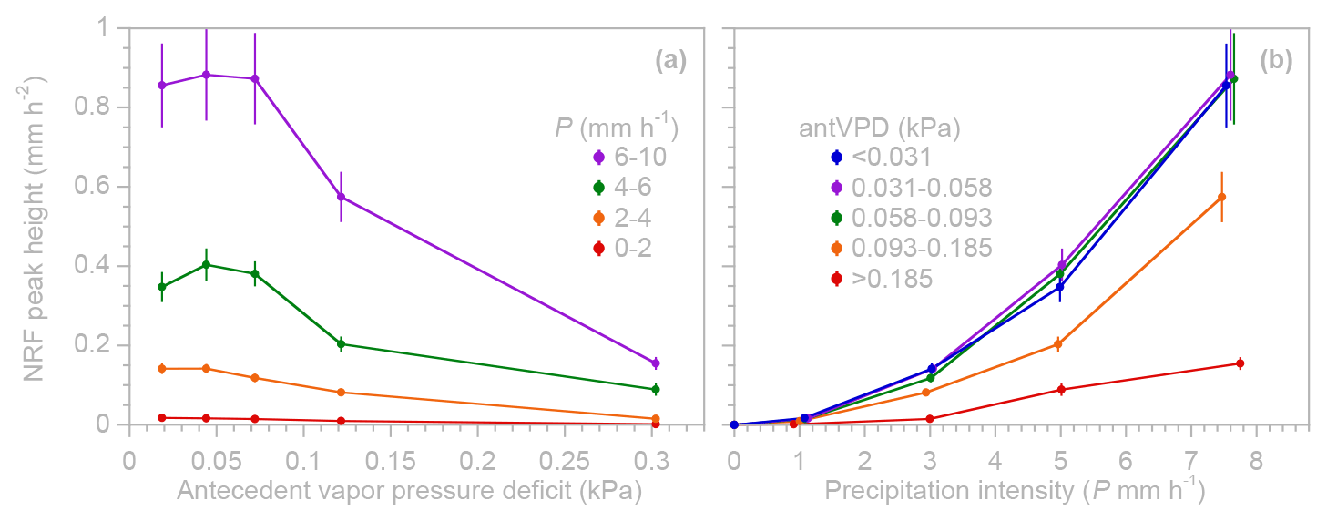
Figure 14 Peak runoff response at Hafren as a joint function of precipitation intensity P and 1 h antecedent vapor pressure deficit (antVPD) without accounting for the co-variation between VPD and antecedent wetness. (a) Peak height of the nonlinear response function (NRF) as a function of vapor pressure deficit for four ranges of precipitation intensity (shown by different colors). (b) Peak height as a function of precipitation intensity for five ranges of antVPD (shown by different colors), corresponding to quintiles of the VPD distribution. Precipitation intensity ranges are more limited than in Figs. 12 and 13 to provide enough time steps for each combination of P and antVPD. Error bars indicate 1 standard error, where this is larger than the plotting symbols. High levels of antecedent VPD appear to reduce runoff response by roughly 80 %, including when precipitation intensity is high.

The need to jointly quantify the influence of multiple correlated drivers can be illustrated by considering the question of how the vapor pressure deficit (VPD) can influence runoff response to precipitation. One may expect that a higher VPD will lead to faster evaporation of incoming precipitation and, thus, to a smaller runoff response. But how big is this effect? To exclude the direct effects of precipitation itself on VPD (whenever rain is falling, the atmosphere is likely to be close to saturation, and, thus, VPD is likely to be low), here, I analyze antecedent VPD (antVPD), the VPD measured during the time step before rain falls. However, even so, one may expect antecedent VPD to be correlated with precipitation rates, partly because hours of rain tend to follow other hours of rain. Between the lowest 60 % and the highest 20 % of VPD in the Hafren data, mean P decreases from 0.44 to just 0.02 mm h⁻¹. Thus, clearly, just as with antecedent wetness in Fig. 13 above, accurately assessing the effects of antecedent VPD and precipitation intensity will require analyzing them jointly, as outlined in Eq. (16). As we will see below, this will also require accounting for the co-varying effects of antecedent wetness, but, as a cautionary tale, I first show what happens when this confounding factor is overlooked.

Figure 14 presents a first attempt at analyzing the joint influence of antecedent VPD and precipitation intensity on NRF peak height at Hafren using five bins of antecedent VPD, each accounting for 20 % of the data. The ranges of precipitation intensity analyzed in Fig. 14 are different from those in Figs. 12 and 13 to ensure sufficient numbers of precipitation events in each combination of precipitation intensity and antecedent VPD. Both panels of Fig. 14 suggest that the lowest 60 % of antecedent VPD has little effect but that, in the upper 40 % (and particularly in the highest 20 %) of antecedent VPD, runoff response is reduced by roughly a factor of 5 relative to the lowest 60 % of VPD, even at the highest precipitation intensities (compare the red curve with the blue, purple, and green curves in Fig. 14b).

This effect is surprisingly large, and a moment's reflection gives a good clue as to why. Periods with high VPD tend to be dry in other ways as well; in particular, weather conditions that lead to higher VPD will also usually lead to low antecedent wetness in the landscape, and, conversely, wetter landscapes will promote faster evaporation and thus reduce VPD. Between the lowest 60 % and the highest 20 % of VPD in the Hafren data, mean antecedent discharge decreases from 0.27 to 0.11 mm h⁻¹, and between the same VPD ranges, the 98th percentile of antecedent discharge (corresponding to the wettest landscape conditions) decreases by a factor of 3, from 1.56 to 0.49 mm h⁻¹. Thus antecedent wetness may be a confounding variable that amplifies the apparent effect of VPD variations on runoff response.

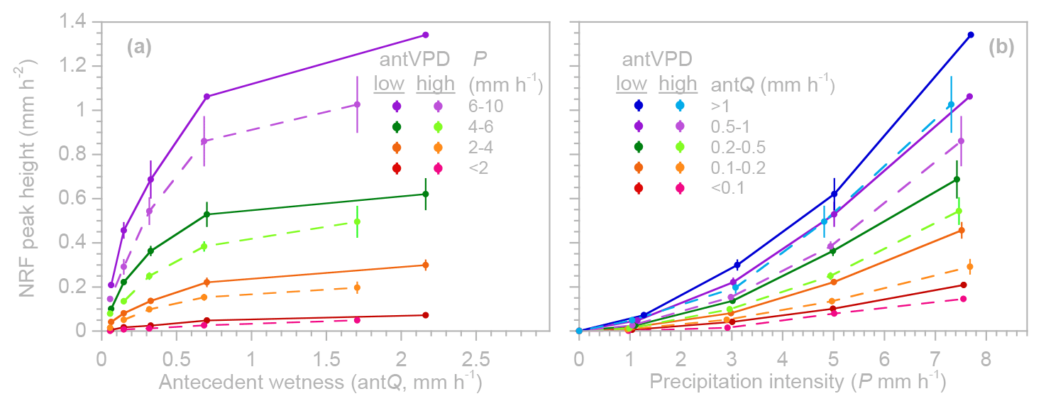
Figure 15 Peak runoff response at Hafren as a joint function of precipitation intensity P and antecedent wetness (using 1 h lagged discharge, antQ, as a proxy) for low antecedent vapor pressure deficit (antVPD) conditions (darker colors and solid lines: lowest 60 % of VPD values) and high antVPD conditions (lighter colors and dashed lines: highest 40 % of VPD values). (a) Peak height of the nonlinear response function (NRF) as a function of antecedent wetness for four ranges of precipitation intensity (shown by different colors). (b) Peak height as a function of precipitation intensity for five ranges of antecedent wetness (shown by different colors). Precipitation intensity ranges are more limited than in Figs. 12 and 13 to provide enough time steps in each combination of P and antVPD. Error bars indicate 1 standard error, where this is larger than the plotting symbols. Jointly accounting for the effects of precipitation intensity and antecedent wetness shows that, all else being equal, peak runoff response is roughly 20 %–30 % lower following periods of high VPD (dashed lines) than following periods of low VPD (solid lines). However, peak runoff response following both low and high VPD exhibits similar dependencies on antecedent wetness and precipitation intensity.

In such cases, seeing the effect of VPD variations will require analyzing them jointly with variations in both antecedent wetness and precipitation intensity. ERRA can do this seamlessly, setting up Eq. (16) to solve for the nonlinear effects of precipitation intensity in nonstationary systems described by any desired combination of drivers – in this case, two ranges of VPD (the lowest 60 % and highest 40 %) crossed with five ranges of antecedent discharge. Accounting for both antecedent VPD and antecedent wetness yields markedly different results than those in Fig. 14. As Fig. 15 shows, runoff response in high-VPD conditions (dashed lines, lighter colors) is reduced by roughly 20 %–30 % relative to runoff response in low-VPD conditions (solid lines, darker colors) but broadly follows the same patterns of dependence on antecedent wetness and precipitation intensity. Thus, one can infer that, as hypothesized, the large apparent effects of VPD in Fig. 14 are not realistic but instead arise from the co-variation between VPD and antecedent wetness.

As the Hafren time series is used to estimate more relationships – first with just antecedent discharge in Fig. 12a; then with antecedent discharge and precipitation intensity in Figs. 12 and 13; and then with antecedent discharge, antecedent VPD, and precipitation intensity in Fig. 15 – the error bars grow. This reflects widening parameter uncertainties as the information contained in the precipitation and streamflow time series is diluted among coefficients for more and more variables, particularly for those that, like VPD and antecedent wetness, are interrelated. Very humid landscapes like the Welsh setting of the Hafren catchment are hardly ideal for measuring how atmospheric vapor demand influences hydrological behavior. Nonetheless, it is reassuring that, even here, ERRA can measure such effects directly from data by analyzing them jointly with potential confounding factors.

5 Quantifying multiscale runoff response spanning both short and long lag times

5.1 Introduction

Streamflow response to precipitation spans a wide range of time scales, often rising to a peak within minutes or hours, followed by a recession that potentially lasts days, weeks, or months. The analysis presented above has focused on short-term responses to streamflow (as most rainfall–runoff analyses do). However, long-tail recession behavior can potentially give interesting insights as well (for example, into catchment storage dynamics; e.g., Kirchner, 2009; Tashie et al., 2019, 2020) if it can be accurately quantified. A challenge in recession analysis is that recessions rarely last more than a few days before they are disrupted by new precipitation inputs. In principle, ERRA should be able to filter out the effects of overlapping precipitation inputs if the runoff response (RRD or NRF) is accurately estimated. However, while this approach solves one problem, it also creates another because accurately portraying the long tails of streamflow recession requires accurately estimating the much quicker and much larger short-term response to precipitation. How can we capture both the quick, high peaks of runoff response and the long tails? If we use time steps that are too long, we will fail to capture the short-term response accurately. But if the time steps are short instead, we will need lots of them, leading to computational inefficiency and also to statistical inaccuracy because (for example) the effects of 1 h of precipitation will be nearly identical at lags of 499 and 501 h, making estimates of coefficients at both lags unreliable.

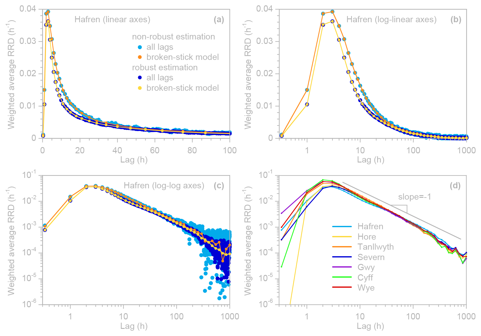
Figure 16 Long-tail recession behavior at Hafren and six other Plynlimon streams. Panels (a–c) show precipitation-weighted average runoff response distributions (RRDs) for Hafren on linear, log–linear, and log–log axes, respectively. In contrast to the other figures in this paper, error bars are not shown here so that the scatter among the points is more clearly visible. Each of these panels shows RRDs calculated at every lag using non-robust and robust estimation (light blue and dark blue, respectively) and RRDs calculated using a piecewise-linear broken-stick model over a geometric progression of lag intervals using non-robust and robust estimation (orange and yellow, respectively). At larger lags, the broken-stick approach averages the runoff response over longer lag intervals, thus greatly reducing the scatter in the long tail of the RRD. Robust estimation further reduces the scatter in the RRD tail by limiting the influence of individual data points with large residuals. Panel (d) shows robust broken-stick RRDs for seven Plynlimon streams. All seven streams have recession limbs that scale as approximately τ⁻¹ over more than 2 orders of magnitude in lag time τ.

Since the hydrological response changes rapidly soon after rain falls and then changes slowly thereafter, we would like to approximate that response with a function that does the same thing. However, in keeping with the philosophy behind ERRA, we want a nonparametric approach rather than one that requires specifying the form of a nonlinear function a priori and estimating its parameters using nonlinear regression techniques. Using techniques described in Sect. 6 of K2022, ERRA can approximate a catchment's runoff response over multiple timescales using a piecewise-linear broken-stick function that has closely spaced knots at short lag times and widely spaced knots at long lag times (Fig. 16). Each knot represents a weighted average of the runoff response over the range of lag times that are closest to it.

The general approach, as described in detail in K2022, assumes that the runoff response coefficient β_k varies linearly as a function of lag time between pairs of knots with (for example) values of ${\mathit{\beta }}_{\mathrm{3}}^{\ast }$ and ${\mathit{\beta }}_{\mathrm{4}}^{\ast }$ at lags of k=κ₃ and k=κ₄, respectively:

$$\begin{array}{}\text{(17)}& {\mathit{\beta }}_k={\mathit{\beta }}_{\mathrm{3}}^{\ast }\left({\displaystyle \frac{{\mathit{\kappa }}_{\mathrm{4}}-k}{{\mathit{\kappa }}_{\mathrm{4}}-{\mathit{\kappa }}_{\mathrm{3}}}}\right)+{\mathit{\beta }}_{\mathrm{4}}^{\ast }\left({\displaystyle \frac{k-{\mathit{\kappa }}_{\mathrm{3}}}{{\mathit{\kappa }}_{\mathrm{4}}-{\mathit{\kappa }}_{\mathrm{3}}}}\right).\end{array}$$

If expressions of this form are substituted into Eq. (3), the linearly weighted regression coefficients between each set of knots can be replaced by weighted averages of precipitation values around each knot κ_ℓ:

$$\begin{array}{}\text{(18)}& \begin{array}{rl}{P}_{j,\mathrm{\ell }}^{\ast }\approx & {\sum }_{k={\mathit{\kappa }}_{\mathrm{\ell }-\mathrm{1}}}^{\left({\mathit{\kappa }}_{\mathrm{\ell }}\right)-\mathrm{1}}\left({\displaystyle \frac{k-{\mathit{\kappa }}_{\mathrm{\ell }-\mathrm{1}}}{{\mathit{\kappa }}_{\mathrm{\ell }}-{\mathit{\kappa }}_{\mathrm{\ell }-\mathrm{1}}}}\right)P_{j-k}\\ & +{\sum }_{k={\mathit{\kappa }}_{\mathrm{\ell }}}^{{\mathit{\kappa }}_{\mathrm{\ell }+\mathrm{1}}}\left({\displaystyle \frac{{\mathit{\kappa }}_{\mathrm{\ell }+\mathrm{1}}-k}{{\mathit{\kappa }}_{\mathrm{\ell }+\mathrm{1}}-{\mathit{\kappa }}_{\mathrm{\ell }}}}\right)P_{j-k}.\end{array}\end{array}$$

Making this substitution converts Eq. (3) from an equation that estimates coefficients β_k for every lag k based on precipitation inputs P_j−k at each lag to an equation that estimates coefficients ${\mathit{\beta }}_{\mathrm{\ell }}^{\ast }$ for knots at lags κ_ℓ based on weighted averages $P_{j,\mathrm{\ell }}^{\ast }$ of precipitation at lags surrounding those knots:

$$\begin{array}{}\text{(19)}& Q_j={\sum }_{\mathrm{\ell }=\mathrm{1}}^{n_{\mathit{\kappa }}}{\mathit{\beta }}_{\mathrm{\ell }}^{\ast }{P}_{j,\mathrm{\ell }}^{\ast }+\mathit{\alpha }+{\mathit{\epsilon }}_j.\end{array}$$

Equations of the form of Eq. (19) can be solved by the same methods used to solve Eq. (3) once the precipitation values P_j−k have been appropriately transformed to the weighted averages $P_{j,\mathrm{\ell }}^{\ast }$. This implies that any of the methods outlined above for quantifying heterogeneity, nonlinearity, and nonstationarity in runoff response (Sects. 2–4, respectively) can also be applied using the multiscale broken-stick approach outlined here. Readers should note that the methods outlined in Sect. 3 also use piecewise-linear broken-stick models but for quantifying nonlinear runoff response over specified intervals of precipitation intensity rather than for quantifying runoff response over wide ranges of lag times. Some of the notation used above has been recycled from Sect. 3, but these are different broken-stick models used for different purposes.)

5.2 Proof of concept: long-tail recession curves at Plynlimon

Here, I demonstrate how the methods outlined in Sect. 5.1 can be used to estimate the long tails of recession curves using hourly data from Plynlimon (Fig. 11) as a proof of concept. Plynlimon nicely illustrates the challenge of estimating recession behavior because rain there is so frequent; at Hafren, only 10 % of rainless periods are 5 d or longer, and only 2.5 % are 10 d or longer. Thus, there are few uninterrupted recessions of significant length, and so inferring recession behavior on longer timescales will require filtering out the effects of subsequent precipitation inputs, which ERRA is designed to do.

Figure 16a–c shows Hafren's weighted average RRD (that is, accounting for nonlinear effects of variations in precipitation intensity) at all hourly lags up to 1000 h or roughly 6 weeks (light-blue symbols in Fig. 16a–c). The RRD is well constrained (as one might expect from over 300 000 hourly measurements spanning 35 years), but plotting on log–log axes (Fig. 16c) reveals that, even with such an extensive data set, the long tail of the RRD is not well constrained in percentage terms (note also that several values beyond the range of the axis, including values below zero, are not shown). The amplitude of the noise in the RRD is approximately constant across the full range of lags and, thus, constitutes a small fraction of strong signals (like the RRD peak) but a large fraction of weak signals (like the long tail).

Some of this noise can be suppressed by invoking robust estimation, which is implemented as an option in ERRA via iteratively reweighted least squares (IRLS; Holland and Welsch, 1977). Robust estimation results from ERRA must be interpreted cautiously because, like any robust estimation method, IRLS downweights points that deviate from the pattern of behavior exhibited by the bulk of the data and, thus, may mistake high-precipitation points as outliers and limit their influence on the results. This artifact is minimized by applying robust estimation only where, as in Fig. 16, the nonlinear effects of precipitation intensity have been accounted for via the methods of Sect. 3. As the dark-blue symbols in Fig. 16a–c show, robust estimation only slightly reduces the runoff response peak while having the intended effect of substantially dampening the noise in the recession. Nonetheless, the recession remains highly uncertain at long lags.

The uncertainty in the long recession tail is substantially reduced by the broken-stick approach outlined in Eqs. (17)–(19), shown in orange and yellow for non-robust and robust estimation, respectively. In Fig. 16, broken-stick weighted average RRDs are shown for 40 knots that span the full range of lags between 0 and 1000 h in a nearly geometric progression (an exact geometric progression is not possible because each knot must correspond to an integer lag number). The broken-stick estimates closely follow the regularly spaced RRD estimates when the signal is strong and closely follow their average trend when the signal is weak and thus the individual lag estimates are noisy (Fig. 16c).

Figure 16d presents robust broken-stick weighted average RRDs for seven Plynlimon streams with drainage areas ranging from 0.9 to 10.1 km² and with at least 35 years of hourly streamflow data. As Fig. 16d shows, all seven streams exhibit power-law recessions that scale as approximately $Q\sim {\mathit{\tau }}^{-\mathrm{1}}$ over lags τ ranging from roughly 5 h to roughly 1000 h. This behavior is markedly different from the exponential recession that would be expected to result from drainage of linear groundwater reservoirs. In particular, if we estimate the recession timescale as $Q/(-\mathrm{d}Q/\mathrm{d}\mathit{\tau })$, we observe that, for a general power-law recession $Q\sim {\mathit{\tau }}^{-\mathit{\gamma }}$, this timescale increases linearly with the lag time itself:

$$\begin{array}{}\text{(20)}& {\displaystyle \frac{Q}{-\mathrm{d}Q/\mathrm{d}\mathit{\tau }}}={\displaystyle \frac{{\mathit{\tau }}^{-\mathit{\gamma }}}{\mathit{\gamma }{\mathit{\tau }}^{-\mathit{\gamma }-\mathrm{1}}}}={\displaystyle \frac{\mathit{\tau }}{\mathit{\gamma }}}.\end{array}$$

Such recessions, therefore, have no fixed characteristic timescale; instead, in our case with γ≈1, the recession timescale at a lag of 10 h is about 10 h, the recession timescale at a lag of 100 h is about 100 h, and so on. The log–log recession slopes in Fig. 16c are not exactly γ=1; instead, they range from γ=1.07 to γ=1.21, deviating from γ=1 by at least 3 standard errors. The corresponding slopes in a conventional recession plot of $\text{log}(-\mathrm{d}Q/\mathrm{d}\mathit{\tau })$ against logQ (Brutsaert and Nieber, 1977) would be $b=\mathrm{1}+\mathrm{1}/\mathit{\gamma }$, ranging from 1.83 to 1.93.

The log–log recession slope γ can be interpreted in terms of the drainage equation of groundwater storage if one assumes that streamflow recession, particularly at long lag times, is controlled by groundwater seepage alone and is not significantly influenced by evapotranspiration. Following the analysis outlined in Sect. 6 of Kirchner (2009), a recession that scales as $Q\sim {\mathit{\tau }}^{-\mathit{\gamma }}$ with γ>1 implies a storage–discharge relationship of $Q\left(S\right)\sim (S-S_{\mathrm{0}}{)}^{\mathrm{1}/(\mathrm{1}-\mathrm{1}/\mathit{\gamma })}$, where S₀ indicates the groundwater storage at which baseflow would go to zero (which would not be reached in finite time). Note that, for values of γ close to 1, the exponent $\mathrm{1}/(\mathrm{1}-\mathrm{1}/\mathit{\gamma })$ can become quite large (e.g., if γ=1.2, the exponent is 6, and if γ=1.1, the exponent is 11), implying strong nonlinearity in the storage–discharge relationship. If γ<1, a recession that scales as $Q\sim {\mathit{\tau }}^{-\mathit{\gamma }}$ implies a storage–discharge relationship of $Q\left(S\right)\sim (S_{\mathrm{0}}-S{)}^{\mathrm{1}/(\mathrm{1}-\mathrm{1}/\mathit{\gamma })}$, where the exponent is now negative, and S₀ indicates a theoretical upper limit to groundwater storage at which seepage would be infinite. If γ=1, seepage becomes an exponential function of storage, $Q\left(S\right)\sim e^{a(S-S_{\mathrm{0}})}$, where a is the reciprocal of the proportionality constant in $Q\sim {\mathit{\tau }}^{-\mathrm{1}}$ (see Eq. 16 of Kirchner, 2009).

6 Limitations

ERRA must estimate many coefficients because it requires one for each lag (of which there may be dozens or hundreds) or one for each knot if the broken-stick approach of Sect. 5 is used. The number of coefficients is multiplied further if multiple rainfall records are considered simultaneously (Sect. 2), if the rainfall record is divided into ranges of rainfall intensity to evaluate nonlinear runoff response (Sect. 3), or if the rainfall record is split among different time windows or different ambient conditions in order to assess nonstationary behavior (Sect. 4). Estimating so many coefficients naturally raises the question of parameter identifiability and overfitting. How do we know when we have too many coefficients? The short answer is that ERRA's standard error estimates will usually tell us. ERRA calculates standard errors for all of its results, starting with conventional uncertainty analysis in the underlying regressions, followed by first-order second-moment error propagation for any subsequent transformations. Thus, if there are more coefficients than can be estimated reliably, this should be revealed by their standard errors becoming large enough to obscure features of interest in the RRD and the NRF. However, the standard errors may be underestimated if the residual autocorrelation is too strong to be adequately compensated for by the ARMA noise correction procedure, usually because the time steps are too short compared to the timescales over which streamflow varies (if it detects this, ERRA will issue a warning and recommend time step aggregation).

At a minimum, ERRA requires evenly spaced time series of precipitation and streamflow (potentially with some missing values in either variable). But how long should those time series be? The answer will depend on many factors, including the precision of the measurements, the complexity of the analysis that one wants to conduct, the influence of confounding factors, the characteristics of the rainfall forcing (how frequent are precipitation events?), and the characteristics of the system itself (how damped and smoothed is its response?). Broadly speaking, what matters is the balance between the complexity of the analysis that the user wants to conduct and the information contained in the precipitation and streamflow time series. That information content is determined primarily by the number and diversity of precipitation and streamflow events that are visible in the time series rather than its length or the number of points it contains. ERRA works best when it can extract information from many diverse rainfall–runoff events to accurately estimate the ensemble average system response. Although it would be mathematically possible to apply ERRA to individual rainfall–runoff events (and ERRA can optionally perform Tikhonov–Phillips regularization to suppress the resulting overfitting noise), that is not its intended purpose, and the reliability of any such analysis has not been benchmark-tested in K2022 and has not been demonstrated here.

Although the proof-of-concept demonstrations presented here have been based on hourly data, the mathematics of ERRA do not tie it to any particular timescale, and it has been tested with everything from 10 min data to daily data. As shown in Figs. 8–10, changes in the time resolution of the underlying data can reveal some features and conceal others. In general, if the frequency of the underlying data is too high compared to the timescale of the runoff response, the standard errors of the RRD and NRF will be large because the residuals will be strongly autocorrelated, reflecting the difficulty in distinguishing runoff responses at closely spaced lags. Conversely, if the frequency of the underlying data is too low compared to the width of the runoff response peaks, those peaks will be damped by averaging. Furthermore, in low-frequency data, it may become difficult to distinguish between a nonlinear response to variations in precipitation intensity and a nonstationary response to variations in antecedent wetness because (for example) precipitation falling early in the day will contribute to the wetness of the landscape and, thus, to a greater runoff response later in the day. In this example, runoff response to daily averaged precipitation will inherently combine the direct effects of precipitation intensity (in relation to infiltration capacity, for example) and the effects of precipitation on catchment wetness during the same time step.

At the risk of stating the obvious, results from ERRA (or, indeed, from any data-driven technique) will only be as good as the data that are available. While ERRA can do a lot to filter out confounding factors (particularly where the potential confounders have themselves been measured), it will be inherently vulnerable to artifacts in the underlying data. Users are therefore strongly encouraged to visually – not just statistically – inspect their data for problems rather than blindly applying ERRA or other analysis tools. Users are also encouraged to avoid sub-dividing the input data into too many categories or time periods, leaving ERRA with too little information to work with (although this should be evident in the standard errors, which ERRA reports with all of its results). Because ERRA is based on temporal correlations between inputs and outputs, it will likely struggle to identify linkages where those correlations are weak. For example, whereas the temporal correlations between rainfall and streamflow are usually strong, the temporal correlations between snowfall and streamflow are typically much weaker because the timing of snowmelt is highly variable and controlled primarily by energy fluxes to the land surface rather than by precipitation per se. ERRA will not work well (and should not work well) where major variations in streamflow are controlled by drivers that are not accounted for in the input data (e.g., snowmelt, glacier melt, or dam releases).

Users should also take care to ensure that the time series that they use are measured on consistent time bases. This can be more challenging than it might seem because weather and streamflow data may be provided by different agencies using time stamps based on different time zones, sometimes with shifts between summer and winter time. Even daily data sets may be based on different definitions of when a “day” begins and ends: at midnight UTC, at midnight local time, or at some other hour (which may, again, shift between summer and winter time). A further difficulty is that these important details are often poorly documented but can significantly affect the results of ERRA analyses.

7 Applications and outlook

The proof-of-concept demonstrations in Sects. 2–5 show that ERRA provides a powerful, flexible, and widely applicable data-driven framework for quantifying how streamflow is coupled to precipitation, including how that coupling varies with ambient conditions (Sect. 4), with precipitation intensity (Sect. 3), and across the landscape (Sect. 2). These proof-of-concept demonstrations suggest three broad categories of potential applications. First, ERRA could be applied to quantify hydrological responses for purposes of catchment characterization. ERRA quantifies the coupling between precipitation and streamflow (rather than just the statistics of streamflow itself). Thus, in inter-catchment comparisons, ERRA should help in clarifying the effects of differences in landscape characteristics (e.g., soil depth and bedrock lithology) by factoring out potentially confounding site-to-site variability in precipitation patterns. Second, both in site-to-site comparisons and in longitudinal studies at individual sites, ERRA could be applied to quantify how changes in factors like climate, land cover, and land use have altered the coupling between precipitation and streamflow. ERRA could, for example, be applied to distinguish cases where streamflow patterns have shifted because precipitation patterns have shifted and cases where the relationship between precipitation and streamflow has changed. Third, ERRA could be applied to define signatures of hydrological response for comparison with models. Figures 8, 9, 13, 15, and 16 are all “fingerprints” of hydrological behavior that could be quantified from real-world data and then from model simulations to facilitate model–data comparisons. Such targeted approaches for confronting models with data are likely to have greater diagnostic power than goodness-of-fit statistics applied to hydrological time series (Kirchner et al., 1996; Kirchner, 2006).

The illustrative examples presented here have focused on the coupling between precipitation and streamflow, but the underlying mathematical methods are general and could potentially be used to quantify linkages between many other hydrological inputs and outputs. For example, ERRA could be used to explore the coupling between precipitation and groundwater recharge wherever groundwater level time series are accurate enough to allow recharge rates to be estimated from rates of water table rise. Such an approach would help in characterizing how the vadose zone modulates recharge response to precipitation inputs. Alternatively, groundwater recharge and streamflow could be used as the input and output, respectively, to characterize how the saturated zone mediates streamflow response to recharge fluxes. Similarly, changes in soil moisture could potentially be used as measures of infiltration rates, and ERRA could potentially be used to explore their coupling to precipitation patterns and recharge dynamics. Or eddy flux data or sap flow time series could potentially be used within ERRA to explore how evaporation and evapotranspiration respond to precipitation inputs while accounting for vapor pressure deficit and available energy as co-variates. Beyond a purely hydrological focus, runoff response distributions quantified by ERRA could also be combined with transit time distributions quantified by ensemble hydrograph separation (Kirchner, 2019; Kirchner and Knapp, 2020) to estimate the “forward” transit time distribution and to explore how it varies with ambient conditions and precipitation intensity. ERRA could also be used to explore the coupling between precipitation time series and chemical fluxes in streamflow in order to quantify how solute fluxes respond to variations in precipitation forcing and antecedent conditions. Several of these potential applications are currently under investigation.

It should be clear that ERRA is not a simulation model in the conventional sense. The goal of ERRA is analysis and characterization rather than prediction because RRDs and NRFs are, at best, incomplete descriptions of hydrological behavior, even when the nonlinearity, nonstationarity, and spatial heterogeneity in that behavior are accounted for. RRDs and NRFs are aggregated descriptions of behavior, averaged over ensembles of events. Thus, one should not expect them to yield nice goodness-of-fit statistics if they are used for hydrograph prediction. That is not their purpose.

It should also be clear that ERRA is designed as a tool for iterative, hands-on exploration of hydrological data through trial and error with analyses of varying degrees of complexity. Thus, although ERRA is computationally efficient and could be blindly applied to the massive hydrological data sets that are now becoming available, its primary intended purpose is not data mining per se. It is designed for human learning rather than machine learning.

Last but not least, analyses like those presented here should be the beginning, not the end, of a scientific investigation. They characterize how hydrological systems behave but do not explain why, at least not by themselves. Answering “why” questions will require carefully designed hypothesis tests, including those that are encoded in models. Here, too, ERRA can play a role, helping to test alternative models of “why” by comparing their signatures to the signatures of real-world behavior.