Assessing groundwater level modelling using a 1-D convolutional neural network (CNN): linking model performances to geospatial and time series features

Groundwater level (GWL) forecasting with machine learning has been widely studied due to its generally accurate results and low input data requirements. Furthermore, machine learning models for this purpose can be set up and trained quickly compared to the effort required for process-based numerical models. Despite demonstrating high performance at specific locations, applying the same model architecture to multiple sites across a regional area can lead to varying accuracies. The reasons behind this discrepancy in model performance have been scarcely examined in previous studies. Here, we explore the relationship between model performance and the geospatial and time series features of the sites. Using precipitation (P) and temperature (T) as predictors, we model monthly groundwater levels at approximately 500 observation wells in Lower Saxony, Germany, applying a 1-D convolutional neural network (CNN) with a fixed architecture and hyperparameters tuned for each time series individually. The GWL observations range from 21 to 71 years, resulting in variable test and training dataset time ranges. The performances are evaluated against selected geospatial characteristics (e.g. land cover, distance to waterworks, and leaf area index) and time series features (e.g. autocorrelation, flat spots, and number of peaks) using Pearson correlation coefficients. Results indicate that model performance is negatively influenced at sites near waterworks and densely vegetated areas. Longer subsequences of GWL measurements above or below the mean negatively impact the model accuracy. Besides, GWL time series containing more irregular patterns and with a higher number of peaks might lead to higher model performances, possibly due to a closer link with precipitation dynamics. As deep learning models are known to be black-box models missing the understanding of physical processes, our work provides new insights into how geospatial and time series features link to the input–output relationship of a GWL forecasting model.

1 Introduction

Understanding the dynamics of groundwater levels over time has gained greater importance in recent years as a key tool for groundwater management. This importance is driven by the link between groundwater discharges to streams, where even slight declines can significantly affect the environment, as highlighted by de Graaf et al. (2019). Various modelling approaches are valuable for estimating groundwater levels in both the short and long term. These approaches allow for the identification of over-exploitation based on depletion trends (Daliakopoulos et al., 2005), enhance our knowledge of water availability for drinking-water supply and agricultural irrigation (Takafuji et al., 2019), and help delineate potential soil subsidence zones due to extremely low groundwater levels associated with droughts and water abstraction (Xu et al., 2008). Furthermore, understanding these dynamics is crucial for sustainable groundwater management in the face of climate change and increasing water demands (Famiglietti, 2014).

Physical and numerical approaches have been widely used as the primary tool to study groundwater level (GWL) (Goderniaux et al., 2015). However, achieving a desired model calibration and/or validation requires extensive physical knowledge of the study area and large volumes of data related to the aquifer properties, geology, and topography, among others. In the last 2 decades, many publications have shown that data-driven models are simpler and faster to develop and provide more accurate results than physical or numerical models under certain conditions (Tao et al., 2022; Malik and Bhagwat, 2021; Ahmadi et al., 2022). Data-driven models using machine learning (ML) techniques such as artificial neural networks (ANNs) have proven their suitability for GWL forecasting (Wunsch et al., 2022) and their ability to capture the non-linearity of the aquifer's dynamics, although this is at the expense of having a physical understanding of the process. Many studies address the former challenge by applying explainable AI methods such as SHAP to elucidate the input–output non-linear dynamics (Chakraborty et al., 2021; Zhang et al., 2023; Liu et al., 2022). In particular, ANNs are suitable for solving groundwater-related problems on a regional scale due to their low dependency on field data accessibility. Many ANN approaches have been successfully implemented, and recent developments in the field of deep learning (DL) promise a significant improvement in the already existing prediction approaches. High overall performances have been obtained through ANN techniques including feed-forward neural network (FFNN) (Roshni et al., 2020), long short-term memory (LSTM) (Wunsch et al., 2021), and convolutional neural network (CNN) models (Mohanty et al., 2015; Ahmadi et al., 2022; Wunsch et al., 2022). Besides DL techniques, shallow recurrent networks such as non-linear auto-regressive networks with exogenous input (NARX) have proven to be useful for modelling a wide variety of dynamic systems (Guzman et al., 2017; Zanotti et al., 2019; Fabio et al., 2022). Regarding accuracy and calculation speed, the CNN models outperform the LSTM. NARX models performed, on average, better than CNN models (Wunsch et al., 2021), mainly because NARX models capture temporal dependencies on groundwater. However, the CNN model has been shown to be faster with only a slightly lower accuracy (Wunsch et al., 2021). Most groundwater modelling has traditionally employed the previously described approaches as single-station models. However, recent studies (Heudorfer et al., 2024) have introduced a global model incorporating multiple stations and static features. Despite this advancement, the performance improvement is modest compared to the progress seen in surface water modelling (Kratzert et al., 2024).

Most studies have successfully applied these techniques for GWL forecasting using meteorological variables as inputs. To date, research has focused on a comparative analysis among different AI techniques, resulting in slight differences among models' performances (Wunsch et al., 2021) or in an improvement in the model's accuracy as a result of modifying its architecture (Gong et al., 2016). In many cases, disregarding site geospatial characteristics can reduce model accuracy or credibility, owing to the different responses depending on the aquifer characteristics (Kløve et al., 2013), unsaturated-zone conditions, and groundwater-contributing area (Rust et al., 2018). Therefore, it is known that, in order to achieve more accurate results in areas influenced by natural and anthropogenic factors, river water level and human impact factors such as pumping rates should be considered as inputs (Lee et al., 2019). For instance, Gholizadeh et al. (2023) applied an LSTM model including static input features (e.g. hydraulic conductivity and soil depth) in an attempt to model ungauged locations; the authors attribute the satisfactory model performance to such inputs. However, as highlighted by Tarasova et al. (2024), the lack of agreement when it comes to evaluating hydrological catchment descriptors hinders consensus on what are considered to be relevant geospatial features, particularly for subsurface characterization.

Since regional studies frequently lack supplementary information beyond meteorological data, this study explores the link between model performance (using only precipitation (P) and temperature (T) as inputs) and site-specific and time series features that might help to understand the input–output relation of a GWL DL model. Although many types of ANN structures have been developed for GWL forecasting, a 1-D CNN (LeCun et al., 2015) is applied here to evaluate the model performance due to its flexibility, calculation speed, and reliability. The model is trained, validated, and tuned individually in 505 wells distributed throughout the state of Lower Saxony, Germany. The research considers geospatial and time series features based on their availability and potential impact on groundwater records. New insights are provided about the complexity of controlling factors on the groundwater dynamics.

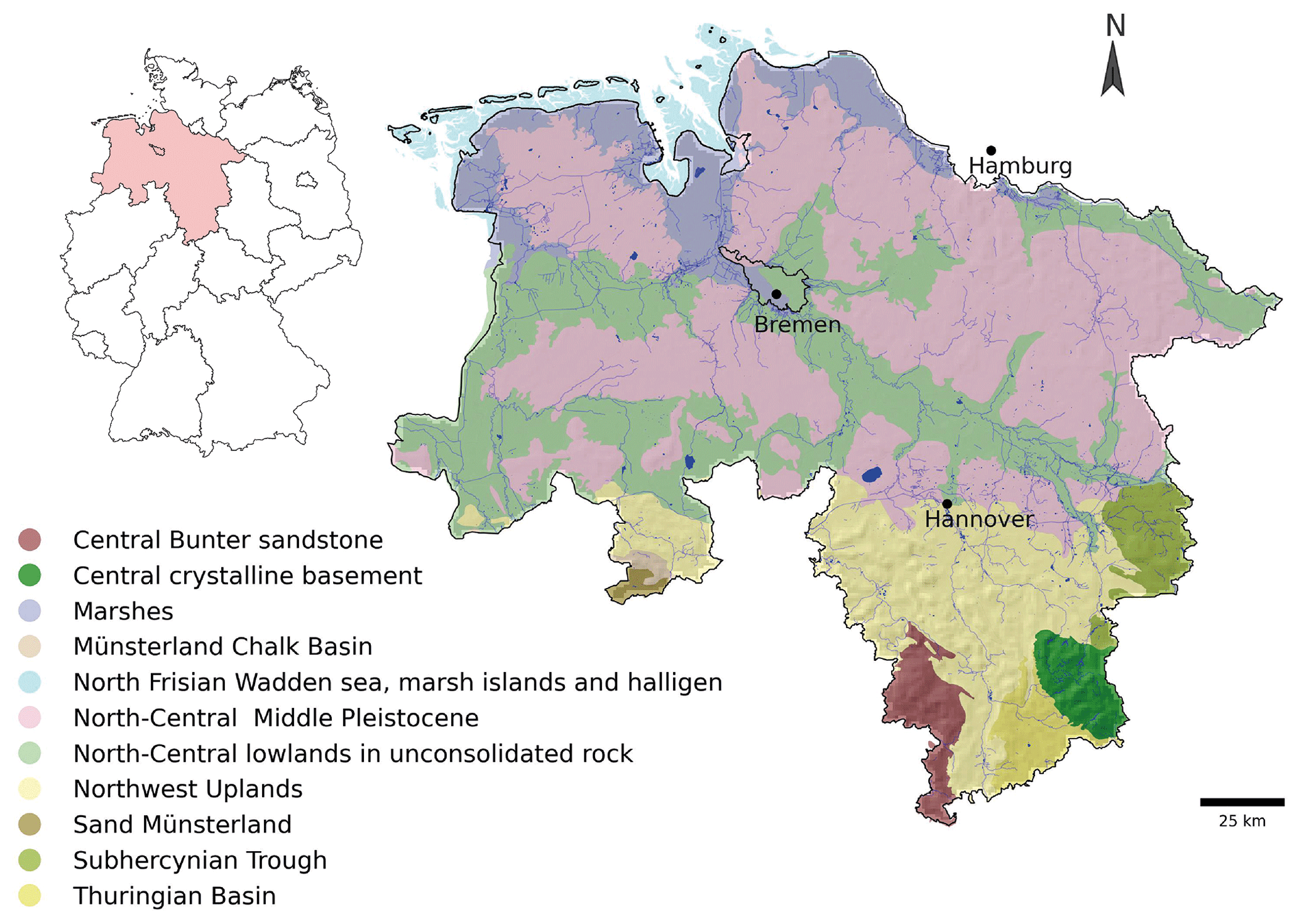
Figure 1 Hydrogeological areas of Lower Saxony: 1:500 000 (modified from LBEG, 2016). The hydrological bodies towards the north correspond to porous aquifers (nord- und mitteldeutsches Mittelpleistozän (north-central Middle Pleistocene), Niederungen im nord- un mitteldeutschen Lockergesteinsgebiet (north-central lowlands in unconsolidated rock), Nordseemarchsen and Nordseeinseln und Watten (North Frisian Wadden Sea, marsh islands, and halligen)). The south consists of fractured and karst aquifers (mitteldeutscher Buntsandstein (central Bunter sandstone), mitteldeutsches Grundgebirge (central crystalline basement), Münsteländer Kreidebecken (Münsterland chalk basin), nordwestdeutsches Bergland (northwestern Uplands), Sandmünsterland (sand Münsterland) and Subherzyne Senke (Subhercynian Trough)).

Rauthe et al. (2013); Frick et al. (2014)

Table 1 Data availability overview.

2 Study area and materials

2.1 Study area

The study area is located in Lower Saxony, Germany (Fig. 1), where groundwater accounts for 86 % of the public water supply (LSN, 2016). The groundwater bodies in this area comprise a great extension of highly productive porous aquifers and, in a lower proportion, fractured hard rock and karst aquifers (LSN, 2016). The landscape is mainly dominated by the lowlands in the northern and central regions, whereas the south is predominantly hilly and mountainous. Land use corresponds mainly to farming (∼ 47 %) and pasture (∼ 15 %), concentrated in the western and northern regions (NMUEK, 2015). The maritime influence in the coastal region affects the precipitation distribution, decreasing from the west (approx. 750 mm yr⁻¹) to the east (< 600 mm yr⁻¹). In contrast, the annual precipitation exceeds 1500 mm in the south (NMUEK, 2015).

From a broad perspective, the northern German Plain is covered up to the edge of the low mountain range by glacial deposits of varying thicknesses (LBEG, 2016), constituting a great proportion of Lower Saxony. Hard rock areas in the southern highlands are formed by sandstones and limestones (BGR, 2019a). Highly heterogeneous geological structures exist among these two groups, leading to groundwater availability at different depths with varying yields, especially in karst aquifers (LBEG, 2016). The primary pressures on the quantitative status of groundwater bodies arise from its long-term abstraction, mainly for drinking water, irrigation, mining or construction activities, and long-term hydraulic measures for groundwater remediation (NMUEK, 2015).

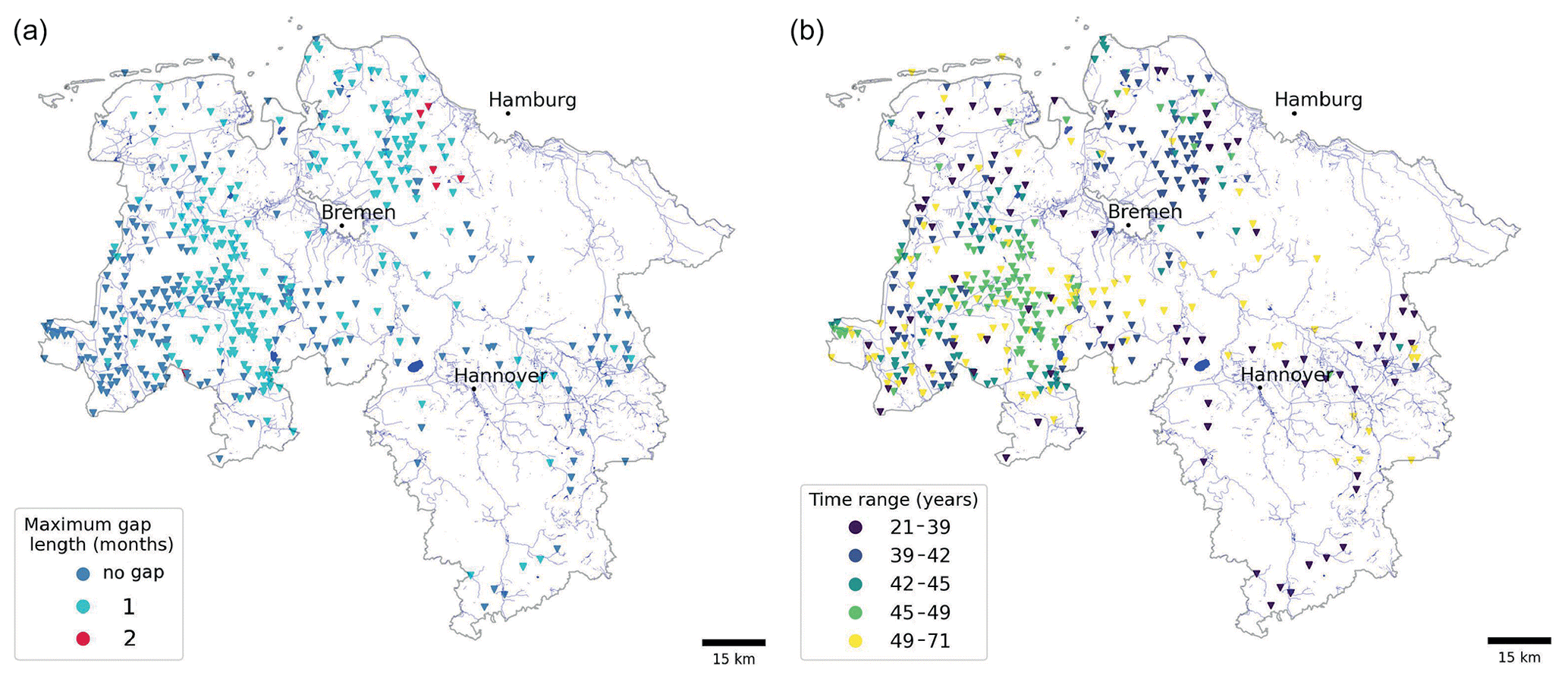
Figure 2 Location of the 505 wells with GWL time series observations used in the study. (a) Maximum gap length and (b) time range of the GWL time series. Author-generated map.

2.2 Data

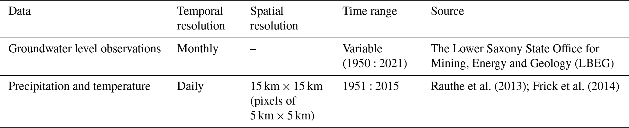
GWL observations and meteorological information are available throughout the state of Lower Saxony. Table 1 shows the data overview. The GWL is at a monthly resolution with a variable time range, and historical records of meteorological variables are available at a daily resolution of 5 km × 5 km. The GWL time series consists of 505 wells that are unevenly distributed, with more information available in the central region of the study area. Besides the irregular spatial distribution, there are data gaps depending on the well (Fig. 2a), and the time range of the groundwater records varies between 21 and 71 (Fig. 2b) years from 1950 to 2021, resulting in differences in the start–end dates of the time series (Fig. A1 in the Appendix).

Figure 3 The bar plots show the distribution of well characteristics in the study area: (a) aquifer type, (b) aquifer material (BGR, 2019b), (c) geomorphology (SMI: soil moisture index) (BGR, 2006), and (d) CORINE land cover (Copernicus, 2018).

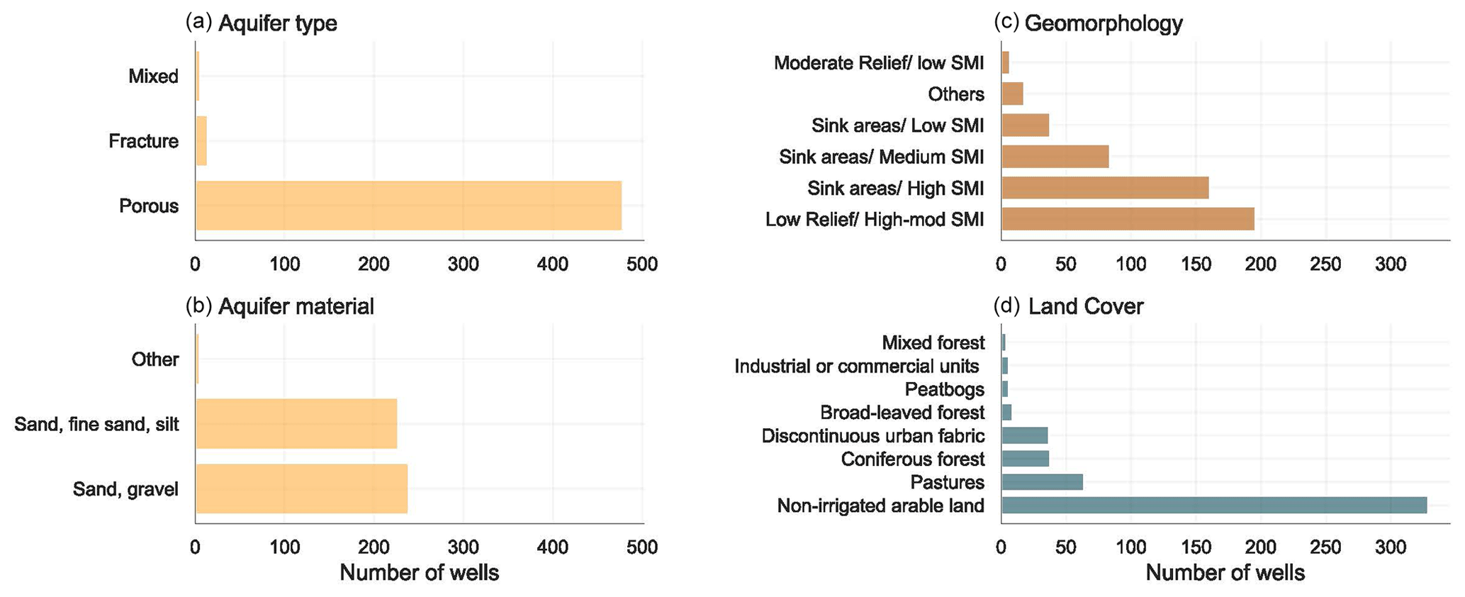
As observed in Fig. 3a, fewer data are available for fractured aquifers, limiting the interpretation in terms of different hydrogeological units. This uneven spatial distribution of the wells reflects the differences in hydraulic properties between porous and fractured aquifers. In the latter, water primarily flows through conduits and cavities, creating a more complex system that could increase the construction and maintenance costs of wells, reducing their number in the area. Almost half of the wells are located in sandy-gravel material (Fig. 3b), associated with high hydraulic conductivity and stronger variations of GWL. The other half of the wells are in finer materials but still with a high sand portion. Regarding geomorphology, the predominant category is low relief with a high to moderate soil moisture index (SMI), followed by sink areas with a high SMI (Fig. 3c). The SMI serves to measure how wet or dry the soil is at any given time based on the minimum and maximum moisture levels that the soil can hold (Hunt et al., 2009). Most wells are in non-irrigated arable lands and pastures (Fig. 3d). Overall, the study area characteristics associated with each well are relatively homogeneous in terms of hydrogeology, geomorphology, and land use. Most wells are located below 100 m.a.s.l. (northern area), and higher elevations relate to wells in the southern mountainous regions. According to the filter depth, most analysed wells relate to shallow aquifers (Fig. A2).

Figure 4 Methodological flow chart.

The historical records of meteorological information in Germany are available as an observational dataset (HYRAS dataset, Rauthe et al., 2013; Frick et al., 2014). This corresponds to gridded hydrometeorological information based on a compilation of variables across Germany and adjacent river basins (Razafimaharo et al., 2020). The dataset consists of daily precipitation (interpolated according to Rauthe et al., 2013) and temperature from 1951 to 2015. The German Weather Service (DWD) adapted and improved the raster data based on more than 1300 stations and with a direct station–grid comparison, making the data highly reliable (Razafimaharo et al., 2020). The daily dataset is provided free of charge for academic and non-commercial purposes (, ).

3 Methods

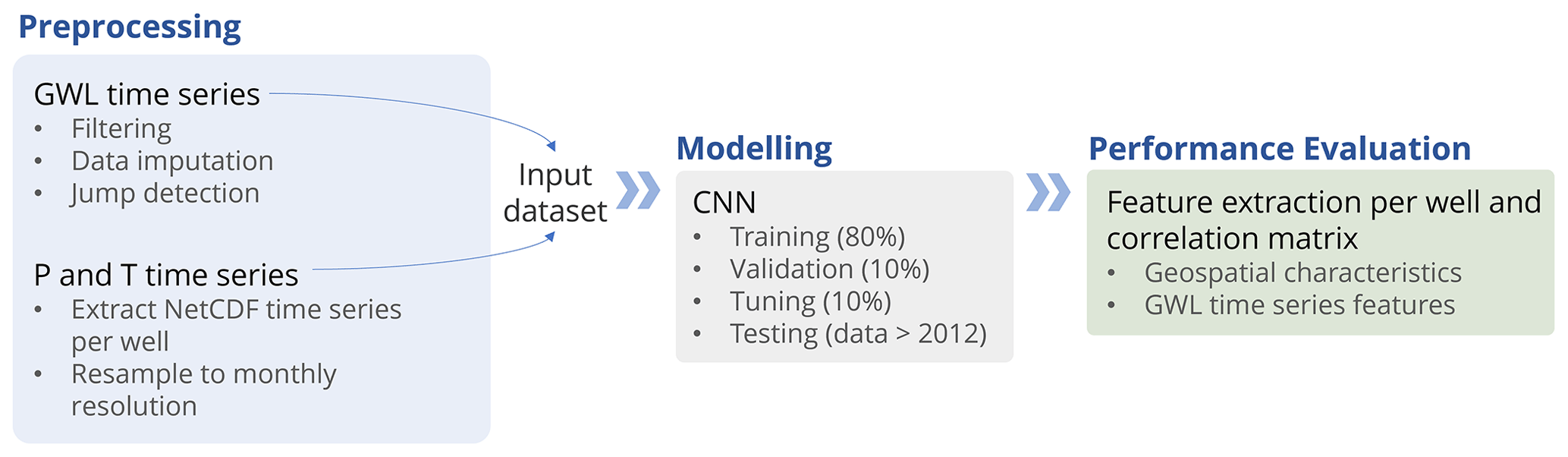
Figure 4 presents the methodological flow chart. the first stage consists of pre-processing the available information jointly with exploratory data analysis and data mining. The procedure starts with the GWL observations involving the filtering, data imputation, and jump detection steps. Simultaneously, the meteorological variables are extracted per well location and are re-sampled from a daily to monthly resolution. As a result, there is an input dataset per well relating GWL, P, and T. In the second stage, a CNN model is implemented, validated, optimized, and tuned through a Bayesian optimization process (Snoek et al., 2012; Nogueira, 2014). The latter corresponds to an optimization method based on Bayesian inference and a Gaussian process to maximize the sum of performance metrics, in this case the Nash–Sutcliffe efficiency (NSE) and R². The following step is concerned with the performance evaluation and interpretability, relating geospatial and time series features with the performance metrics. To achieve the objectives, several Python libraries are used, namely pandas 2.0 (Reback, 2020), NumPy 1.23 (Van Der Walt et al., 2011), SciPy (Virtanen et al., 2020), Matplotlib (Hunter, 2007), GeoPandas 0.14 (Jordahl et al., 2020), and TensorFlow 2.7 (Abadi et al., 2015) as the most relevant throughout the process. Additional specific libraries are mentioned later for each methodological step.

3.1 Pre-processing

The initially available GWL information consists of 962 wells. A pre-selection was done based on the categorization performed by Wriedt and NLWKN (2020), which considered the agreement between theoretical and observed hydrographs, as well as visual indications of anthropogenic influences. This process aimed to exclude wells under strong anthropogenic influences, such as pumping, to better capture the dependency between meteorological input features and observed groundwater levels. After applying this filter, a total of 745 wells remain. A second selection removes time series with gap lengths above two consecutive missing values, obtaining 505 wells, with 241 (48 %) being a complete series, 254 (50 %) having one missing value, and 10 (2 %) having two missing values. To provide the CNN model with continuous time series, we performed data imputation using multiple linear regression (MLR). This method is applied only when the wells exhibit similar behaviour in their time series, as determined by Euclidean distance. The distance is calculated between GWL time series after standardizing each series to be zero-centred with a standard deviation of 1, followed by detrending to remove linear trends. This approach ensures that the comparison focuses on the primary fluctuations in the data. We refined this approach in the analysis, selecting wells with the smallest Euclidean distances (below the 10th percentile) for MLR, ensuring a model R² score above 0.7. If the score is not met, we use the piecewise cubic Hermite interpolating polynomial (PCHIP) for gap filling (Virtanen et al., 2020; Fritsch and Butland, 1984). Overall, the time series have less than 5 % gap-filled values. Additionally, jumps (sudden changes in the time series) are identified at 28 wells and might be associated with measurement instruments or other technical problems (Post and von Asmuth, 2013; Retike et al., 2022). We identified the observations displaying these anomalies by finding the highest slope in the cumulative sum and removing the time series before 1990 for those wells. This is because we are aware of changes due to measurement devices around this time. Finally, to extract the meteorological information, an average of 3 pixels × 3 pixels is used to reduce uncertainty related to the grid cell size following the suggestion of Linke (2017).

3.2 Modelling

The 1- CNN structure is implemented based on Wunsch et al. (2022). This type of network was specifically designed to process and analyse sequential data, capturing local patterns and temporal dependencies through convolutional layers. In this implementation, the input data are scaled between −1 and 1 to enhance the learning process. The inputs are divided into sequences of a defined length. These sequences pass through a 1-D convolutional layer, where a fixed kernel window convolves through the data. The maximum value from each convolution operation is extracted to form the max pooling layer, reducing dimensionality and highlighting the most significant features. To prevent overfitting, a Monte Carlo dropout of 50 % is applied. Following this, a flattened layer converts the pooled features into a one-dimensional array, which is then processed by a fully connected dense layer using the rectified linear unit (ReLU) as the activation function.

The CNN model is applied to each GWL time series, encompassing the phases of training, validation, optimization, and hyperparameter tuning, which are also carried out per well. The available groundwater data prior to 2012 are split between the training (80 %), validation (10 %), and hyperparameter tuning (10 %) dataset, while the 2012–2015 period serves as the test set. Each subset differs depending on the time range of GWL observations, which vary from 21 to 71 years. Thus, the input features, time range, and specific model parameters create a unique representation of the GWL for each location. An Adam optimizer is applied with 100 training epochs, an initial learning rate of 0.001, and the early stopping of 15 patience. In this case, the loss is minimized with the mean squared error (MSE) through each epoch for the validation process. The hyperparameter tuning is done with a Bayesian optimization (Snoek et al., 2012; Nogueira, 2014) to maximize the sum of the squared Pearson (R²) and the Nash–Sutcliffe efficiency (NSE) coefficients, measuring the deviation of observed GWL from predicted GWL over the total observations. The hyperparameters correspond to kernel size (fixed at 3), sequence length (1–12 months), number of filters (1–256), density size (1–256), and batch size (1–256). Owing to the dataset's monthly resolution, the sequence length boundaries are set between 1 and 12 months, a time range that can include significant variabilities in the subsequences. For comparison, we employed a baseline model consisting of a sinusoidal function added to the precipitation trend from the last 9 months. This baseline model was optimized using the same Bayesian optimization method, maximizing the NSE and R² metrics.

OSM (2022)OSM (2022)Copernicus (2018)Copernicus (2022)BGR (2006)Pistocchi (2015)BKG (2021)BKG (2021)Beven and Kirkby (1979)BKG (2021)

Table 2 Overview of geospatial features considered for the performance evaluation.

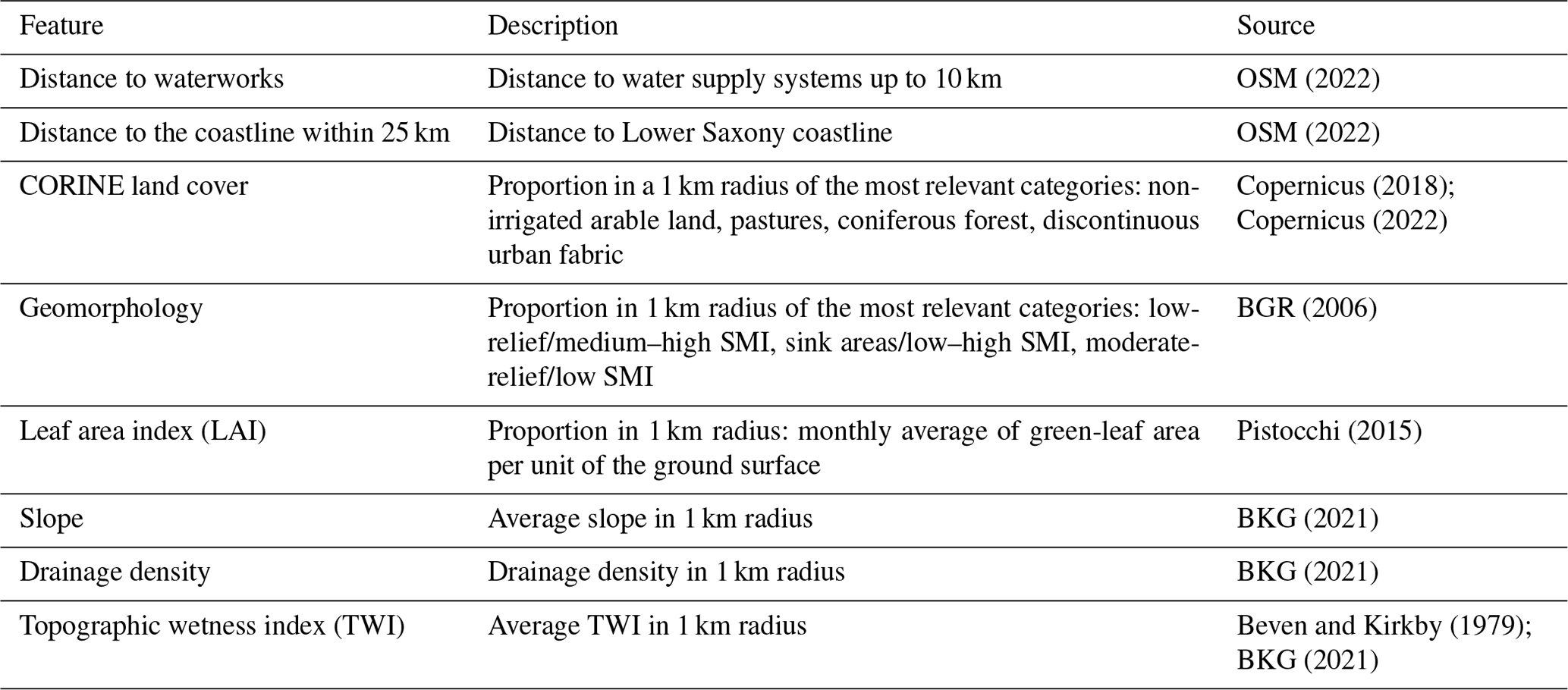
Table 3 Overview of time series features considered for the performance evaluation.

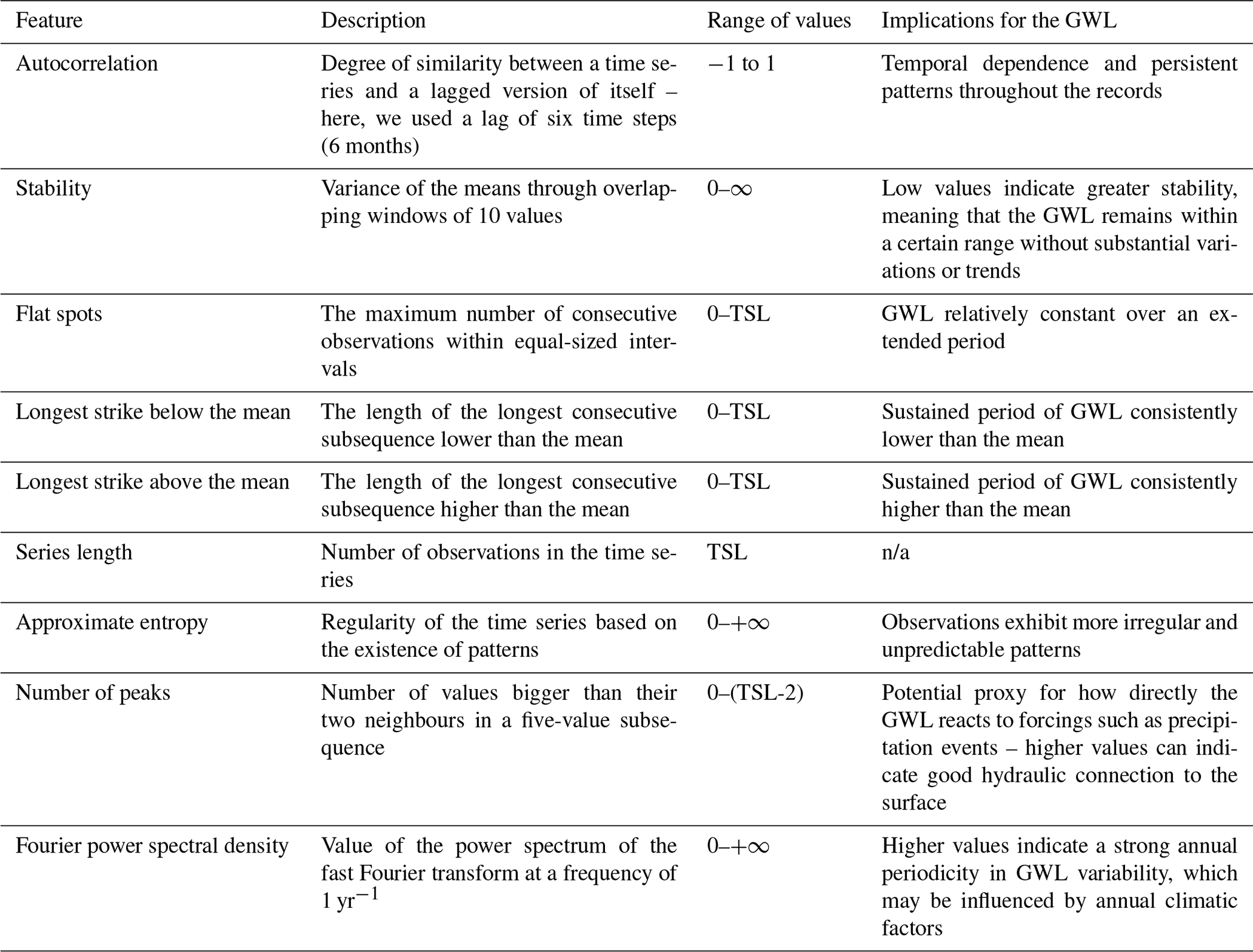
^* TSL – time series length. n/a: not applicable

3.3 Performance evaluation

The model performance can be significantly or slightly affected, depending on the well location, by natural and anthropogenic factors, such as the distance to waterworks or watercourses, the type of land cover, and the geomorphology. Besides, the intrinsic patterns present in the observation time series might reveal external effects on the GWL model. Table 2 describes the geospatial features considered. The selection was made based on data availability and their potential impact on groundwater records. We also performed the analysis with further geospatial features, such as distance to the surface waterbodies, but no statistically significant correlation with model performance was found, and, therefore, the results are not shown here. Among the reported ones, the distance to the waterworks is expected to modify groundwater flow and, consequently, the GWL nearby in the surrounding wells. Here, we assume that Open Street Map (OSM, 2022) includes a significant proportion of all waterworks in the study area, but a comprehensive dataset including the locations of all waterworks or information regarding pumping rates is still missing. Regarding categorical variables, the proportion of a 1 km radius around the well is taken as it has been shown to adequately represent the contributing area of a monitoring site, especially when detailed information about groundwater conditions is lacking (Knoll et al., 2019). The Python packages of tsfeatures (Yang and Hyndman, 2020) and tsfresh (Christ et al., 2018) are used to extract multiple GWL time series features automatically. A selection is made from the long list of features (available in each package) according to their Pearson correlation coefficient in relation to the model performance metrics (R² and NSE) and the value added to the analysis (interpretability in the context of groundwater level). We are aware that Pearson correlations provide linear relationships, and so we also computed Spearman rank correlation coefficients. However, since the Spearman rank did not yield higher correlations, we chose to continue using Pearson correlations. Table 3 shows an overview of the selected time series features, descriptions, and ranges of values, as well as guidelines regarding their occurrence in the GWL time series (for a detailed description of the estimation procedure, please refer to the package manual). We incorporated the Fourier power spectral density over a period of 1 year to measure the influence of annual climate seasonality on the GWL. Higher values indicate a greater annual seasonality. High autocorrelation values indicate patterns constantly repeating in the time series. High stability values imply that GWL remains within a consistent range without significant variations or trends. The more flat spots represent the more relatively constant values over extended periods. Approximate entropy and the number of peaks act as measures of the complexity of the time series. A high value of the former indicates that the GWL time series contains multiple irregular patterns, making it harder to predict. A higher number of peaks indicates multiple local maximums, implying stronger fluctuations in GWL observations.

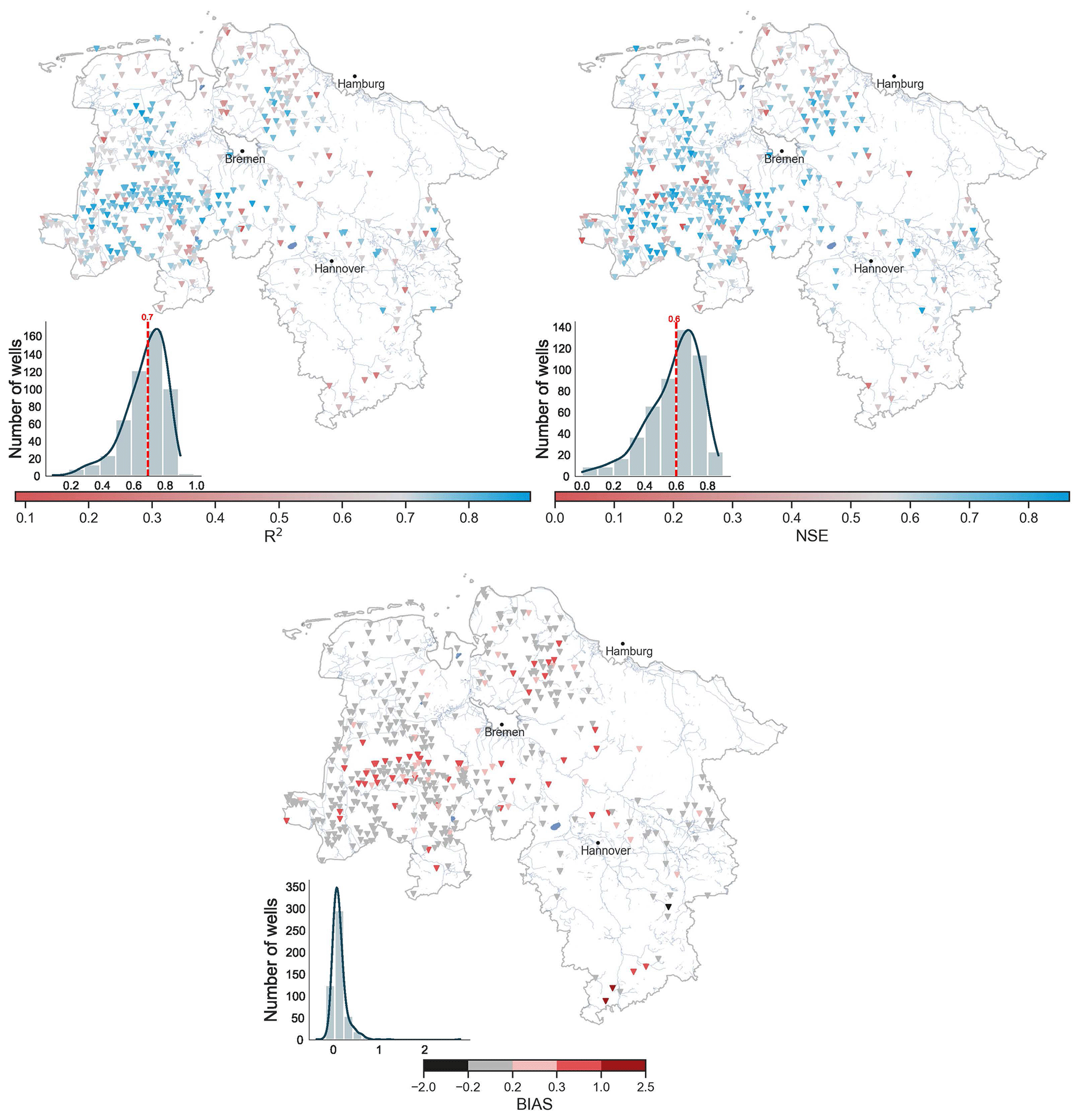
Figure 5 Spatial distribution of model performance metrics (R², NSE, and bias) per well and their respective histogram. Author-generated map.

To evaluate the impact of external factors on the model performance, the geospatial and time series features are extracted per well and are correlated with the accuracy metrics (R², NSE, and bias) through the Pearson correlation coefficient. An R² and NSE value closer to 1 indicate a higher similarity between modelled and observed GWL, whereas the closer the bias is to zero, the more similar the simulations are to the observed data; negative bias refers to a model with underestimation. To enhance the robustness of the correlations, we took the mean correlation coefficient after bootstrap sampling with 100 re-sampling datasets. We report only those correlations that demonstrate statistical significance, ensuring that they fall within a 90 % confidence interval to guarantee the reliability of our findings. The main objective is to notice positive or negative effects on the model performance.

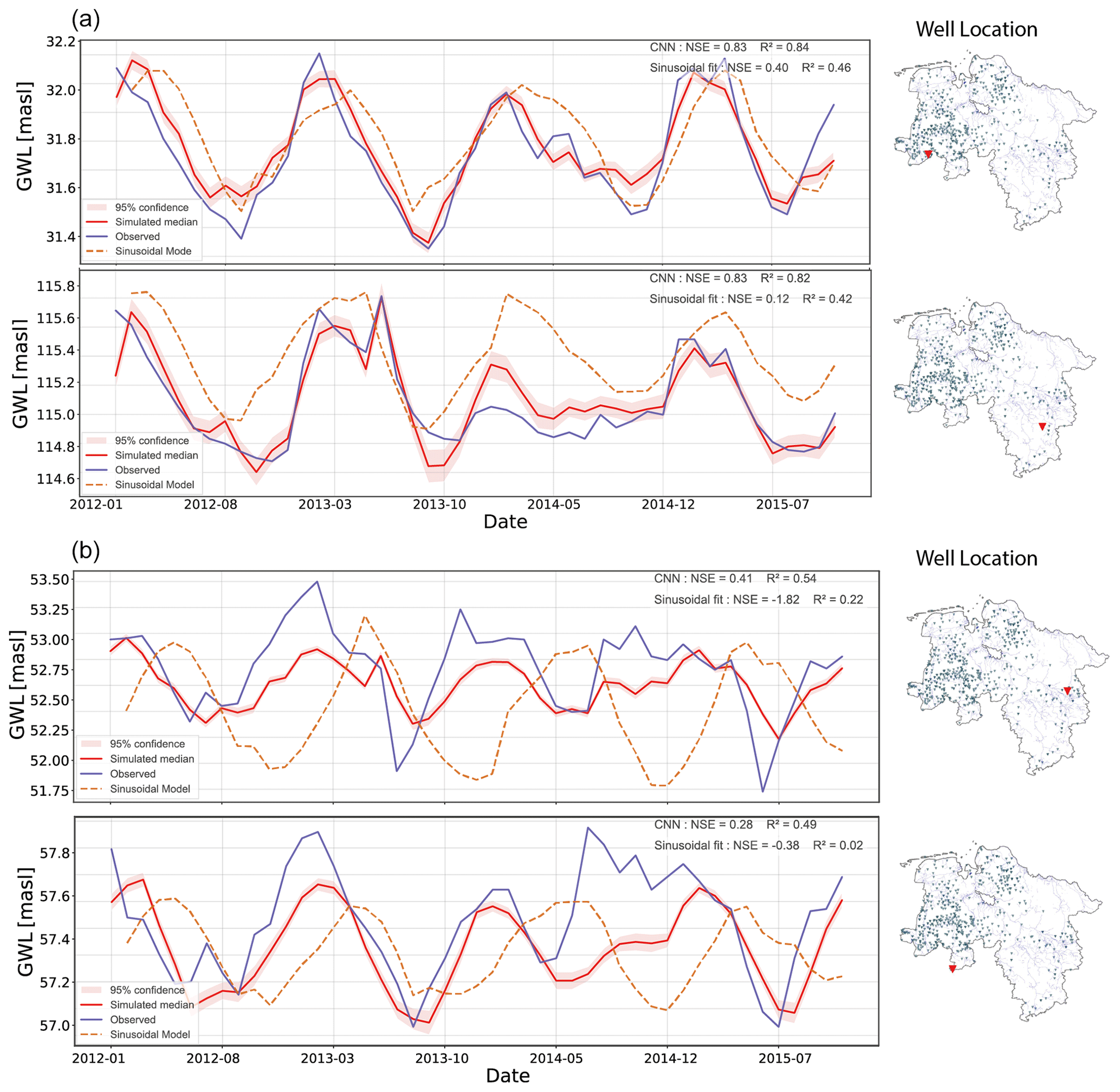
Figure 6 Examples of the observations, CNN model, and baseline model (sinusoidal curve plus precipitation trend) for cases of (a) high performance and (b) low performance.

4 Results

4.1 Modelling

The performance per well is presented in Fig. 5. According to our results, a total of 212 wells show R² and NSE values above 0.7 and 0.6, respectively (Fig. 5), which we would consider to be an acceptable model fit (Moriasi et al., 2015). Lower performance is seen mainly in the south, related to the fractured aquifers, where both metrics (R² and NSE) are below 0.5. The highest positive and negative bias also occurs in those hydrogeological areas. These wells correspond to the shortest data length. Most of the best-performing models are found for the wells in the central region of the study area. Contrarily, some models exhibit low performance near the coast in terms of R² and NSE, with a bias is between ± 0.2.

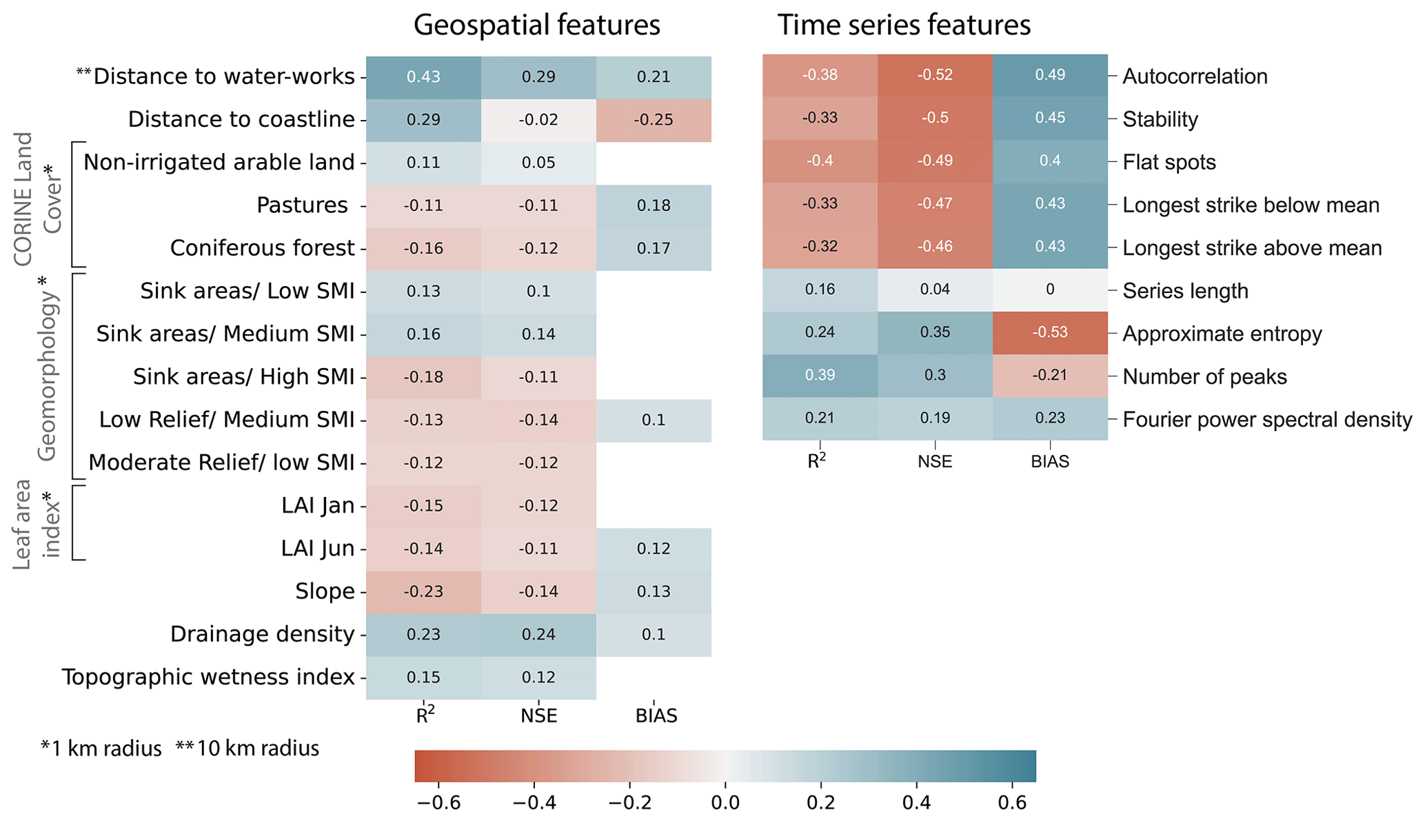
Figure 7 Pearson correlation coefficients between the geospatial features, the GWL time series features, and the model performance. Significant correlations are displayed with a confidence level of 90 %. Blank spaces correspond to non-significant correlations. Correlations with the distance to waterworks are done with 90 wells located in the 10 km buffer and with 50 wells located up to 25 km away from the coastline.

After visually comparing most of the CNN models with GWL observations, a degree of agreement can be noted between the simulated and observed GWL (Fig. A5). Figure 6 shows examples where the optimized model performs well and where the model does not correctly reproduce GWL variability. The baseline model captures the general pattern of GWL fluctuations where the CNN performs better, but it fails to capture smaller variations. The CNN model occasionally underestimates or overestimates the peaks and troughs, particularly struggling with steep peaks, which are often underestimated. In most cases, local variations in the time series are ignored. Occasionally, in poorly performing models, the pattern of the GWL observations has been generally learned but with a strong bias (around 10 % of the wells show a bias above 0.13). The well-performing cases show how the CNN model can represent low peaks for some wells. Additionally, model overfitting is low, as seen in Fig. A3, along with the effects of the lengths of the training, validation, and testing periods, as shown by Fig. A4.

4.2 Performance assessment

The correlation coefficients between the geospatial and time series features and the model performance are shown in Fig. 7. Only significant correlations with a 90 % confidence interval are displayed. Although the correlation coefficients are statistically significant, they do not exceed 0.53 for time series features. Correlations for the geospatial features are weaker, serving, in both cases, more as an indication rather than providing strong evidence. One of the highest correlations is the distance to the waterworks, corresponding to 0.43 (R²) and 0.29 (NSE). Although there is no clear spatial pattern followed by R² and NSE, the Pearson correlation suggests that model performance improves with increasing distance from the coastline. The proportion of the most common land cover type in the study area (non-irrigated arable land) suggests a positive relationship with model performance. Conversely, wells surrounded by significant areas of forest or a high leaf area index (LAI) tend to show lower correlations. Sink and low-relief areas with medium to high SMI may negatively impact performance. Hilly regions might indicate lower accuracy, while areas with high drainage density or a high topographic wetness index suggest better model performance.

Regarding time series features, autocorrelation may reduce model performance. This might not be the case when using antecedent GWL as an additional input feature, where GWL shows the highest influence on model output (Chakraborty et al., 2021), better explaining the current state based on the past one if the time series is highly autocorrelated. Similarly, higher variance of the means through overlapping windows (as indicated by the stability feature defined by Yang and Hyndman, 2020) may reduce model performance. Increasing flat spots and long strikes above or below the mean are negatively correlated, particularly with the NSE metric. Positive correlations are mainly associated with complexity measures such as approximate entropy and the number of peaks. The time series length positively correlates with R² but does not correlate with NSE. Higher values of the Fourier power spectral density at 1 year (indicating stronger annual seasonality in the observed GWL) result in higher model performance.

5 Discussion

The analysed wells are located in a relatively homogeneous area in terms of hydrogeology, associated with a major proportion of porous material and shallow aquifers, improving the model's capacity to express GWL only in terms of meteorological inputs (Kløve et al., 2013). There are a few wells in the fractured and karst aquifers, but those are frequently associated with greater depths (Wunsch et al., 2022). A more diverse distribution of wells is observed with regard to land cover and geomorphology, resulting in distinct interactions between climate, land use, and groundwater (Kløve et al., 2013; Treidel et al., 2011), potentially influencing the model performance.

The primary source of uncertainty in the current analysis is the inability to separate the effects of each external feature affecting observations, particularly geospatial features. This uncertainty is highly dependent on the aquifer size (Kløve et al., 2013), the amount of available information, and the reliability of the information. Furthermore, time resolution may introduce additional uncertainty as the magnitude of GWL fluctuations varies significantly from season to season (Taylor and Alley, 2001). Certain patterns in groundwater dynamics, especially in karst aquifers or those with strong secondary porosity, become more evident at weekly or daily time steps. Consequently, the use of a monthly resolution in our study may not fully capture these dynamics. Additionally, because the vast majority of the wells used in this analysis are located in porous aquifers, our results are primarily representative of these conditions.

The GWL behaviour follows the interactions between climate, topography, hydrogeology, and land use, among others (Earman and Dettinger, 2011). Estimating GWL solely with meteorological variables brings uncertainty, especially in areas with more significant human impacts. Additionally, there are uncertainties related to the model realizations, which, in this case, are solved by using several random initialization seeds. As a result, the model precision is generally high, and we only use the best-performing optimized models. Regarding the geospatial relations with the model performance, there are uncertainties based on the variable scale and the definition of influential radius (assumed to be 1 km for the geomorphology and land use and 10 km for the waterworks), as well as on the reliability of the primary information.

5.1 Modelling

Overall, the CNN model was able to simulate, to a significant extent, the GWL changes for more than 200 wells with good overall performance (R² > 0.7 and NSE > 0.6). Thus, the remaining wells account for at least one metric with non-acceptable performance, and, in those cases, further hydrological or anthropogenic factors might influence the GWL behaviour. The Bayesian optimization currently maximizes the sum of R² and NSE, occasionally causing contrasting values for both metrics at specific wells. Thus, constraining both values to define model performance guarantees adequate results, even when individual accuracy is lower than the acceptable criteria (Gong et al., 2016). Different combinations of metrics can also be explored against model improvements. As explained, Bayesian inference and a Gaussian process (Snoek et al., 2012; Nogueira, 2014) are used to tune the hyperparameters (external parameters that cannot be learned from the data). However, additional tuning strategies such as genetic algorithm and grid search have shown better results (Alibrahim and Ludwig, 2021). Therefore, modifying the optimization strategy and adjusting the network architecture can enhance the results. Alternative networks, such as LSTM or FFNN, may further improve the learning process. However, in this study, our priority is to understand the link between GWL and geospatial and time series features rather than focusing on optimizing the network architecture.

Generalizing the model inputs for all wells throughout the state influences the scores, especially at sites where GWL is not driven by P and T only. Even with a low performance, sometimes, the model can learn the GWL variations but incorporates a bias. Around 10 % of the wells show strong bias (> 0.3), meaning the model has little or no intersections with observations. Differences in spatial resolution between the input data (gridded P and T) and the GWL observations can cause this bias at some stations. When both metrics used for the optimization (R² and NSE) are high, the model is seen to fit the observations adequately. At certain times, the model misses the small spikes on the observations. However, a model that adequately represents the lower and higher periods due to dry or wet years holds higher relevance for groundwater management. Even though the received dataset excluded highly impacted anthropogenic time series, low performance is primarily observed when a significant anthropogenic or non-periodic signal is present in the time series. Models that do not accurately learn from meteorological inputs might be treated independently. Specific external forcings influencing GWL variability might be studied, and particular cases should be re-trained with the additional influencing variables. Lastly, while model overfitting appears to be small (Fig. A3), the low performance on the test data may still be attributed to overfitting at some stations.

5.2 Performance evaluation

The weak correlations between the geospatial features and the model performance can be related to the regional scale of the analysis and to the multiple drivers controlling the GWL at a specific location. Factors such as the spatial resolution of the geospatial features or the large numbers of observation pairs could also reduce the correlation coefficients (Armstrong, 2019). For instance, a skewed probability distribution in the filter depth, which is below 50 m in most wells, excludes deeper aquifers from the analysis and can hinder the relation. Even though we reported a directly proportional relationship between model performance and distance to waterworks, the correlation might be weaker due to non-reported abstractions. However, it is inferred that wells outside the influence area of the waterworks are more prone to being represented by only meteorological variables. Contrarily, wells located in the influence area of the waterworks system should include variables such as abstraction rates to keep the learning process stable (Lee et al., 2019)

The land cover can influence the recharge and the GWL dynamics. When the surface is sealed, the aquifer recharge decreases, and the GWL diminishes. In the same way, groundwater recharge is significantly reduced through evapotranspiration wherever dense vegetation is present, such as in a native forest (Lerner and Harris, 2009). In this case, most wells are located in non-irrigated arable land, which consists of rainfed crops, meaning a more direct response of GWL to meteorological variables is feasible. This supports the positive correlation suggested in Fig. 7 between model performance and wells located in non-irrigated arable land. Contrarily, model performance is reduced as LAI increases. LAI indicates the vegetation canopy, and, therefore, it governs the interception of precipitation, largely controlling the partitioning of infiltrated water into evapotranspiration and percolation (Reichenau et al., 2016). Thus, the interception process can hamper a direct response of GWL to precipitation (Pan et al., 2011), affecting model performance as a result. Regarding geomorphology, areas of accumulation (sink areas) with low to medium SMI positively affect the performance, but this effect is negative when the SMI is high. Sites with higher relief and SMI present lower performance. According to Rajaveni et al. (2017), geomorphological features referring to the accumulation process (pediment and valley fill) have a good groundwater potential and are, therefore, more prone to react to meteorological inputs. Accumulation areas are also represented by the increased drainage density and topographic wetness index (TWI) because these areas are likely to respond quicker to meteorological inputs. We also expected the model's fitness to decrease as the slope increases since steeper areas account for higher runoff, reducing the influence of precipitation dynamics over GWL observations.

As the geospatial characteristics surrounding the groundwater well influence observations, investigating the patterns encountered in the time series by extracting selected features can provide insights into model performance affectations. For instance, the recurrent presence of flat spots on the observations, seen as relatively constant values over extended periods, reduces model performance. This might indicate an aquifer that is less responsive to climate variability, which is often the case with large aquifers (Kløve et al., 2013). We can apply a similar argument to the reduction in performance when there is an increase in time series stability. This means that the GWL remains within a specific range of values without significant variations. Thus, even if there are upward or downward changes in precipitation, the observations of GWL do not exhibit similar patterns. Consequently, the proposed model using only P and T would fail to reproduce the GWL patterns adequately. We found that the learning process is reduced as long consecutive subsequences above or below the mean occur. Direct human influences such as managed aquifer recharge can keep the GWL above the average and modify its response to meteorological variables. The opposite happens when groundwater abstractions exceed recharge and when the aquifer levels drop for a more-or-less-continuous period (Wendt et al., 2020). In both situations, the anthropogenic effects on GWL reduce the performance. Natural climate variability might also result in a similar effect, negatively affecting performance. For instance, if wetter or drier periods occur during testing but not in the training phase, the model is unlikely to learn the consequent patterns. Additionally, the time series complexity measures (approximate entropy and the number of peaks) indicate a directly proportional relationship with model performance, meaning that the more complex the GWL time series is (more irregular patterns), the better the fit is between simulations and observations. Complex GWL time series might reflect a good response to precipitation.

Previous studies have shown little or no correlation between the time series length and the model performance (Wunsch et al., 2021). However, at least, observations over decades are required to cover groundwater dynamics due to climate variability (Taylor and Alley, 2001), especially when considering a monthly temporal resolution. In this sense, the model can incorporate more information into the learning process, and model performance might increase with longer time series. However, conclusions about this relation should be further studied.

6 Conclusions

Fluctuations in the GWL observations are influenced by a combination of natural and anthropogenic factors, challenging the modelling of groundwater systems. An alternative to highly data-requiring physical and numerical models is DL techniques. Many DL models have been applied to GWL modelling, but the main concern with regard to using these models remains a lack of physical understanding. Owing to the complex system between climate, GWL, and external drivers, model performance can be directly or indirectly affected outside of what the model can explain, limited by the input features. Our study brings about insights into how model performance is affected by geospatial features and intrinsic time series characteristics. We selected a 1-D CNN model to simulate monthly GWL time series per well in northern Germany, using P and T as inputs. Our results indicate low performances in wells near waterworks, which is an expected result as GWL is modified by pumping rates. An increased LAI or forest land cover might lead to lower performance by hindering the P and T relation with the GWL. Complex time series relate to a better performance, possibly linked to a closer relationship between GWL and P patterns. More extended continuous GWL measurements above or below the mean negatively impact the metrics and can be associated with artificial recharge, pumping imposed in the time series, or natural events such as wetter and drier seasons. Even though only P and T are used as model inputs, the performances obtained are considered to be acceptable (R² > 0.7 and NSE > 0.6) for more than 200 wells. Nonetheless, incorporating explainable AI techniques in future studies is recommended to enhance the interpretation of the non-linear behaviour between groundwater and its influencing factors.

As the study covers regional areas, local variabilities in climate and human–water interactions might occur. Therefore, model performance should be evaluated at locations with greater data availability to strengthen the current research. Moreover, correlations might vary depending on the model architecture selected or the temporal resolution of GWL observations. For instance, a daily resolution can better include groundwater dynamics showing stronger correlations. Our results encourage the joint analysis of physically related characteristics and DL GWL modelling as an essential path to improve the reliability of data-driven models.

Appendix A

Figure A1 Time range of GWL observations. The blank spaces correspond to missing data.

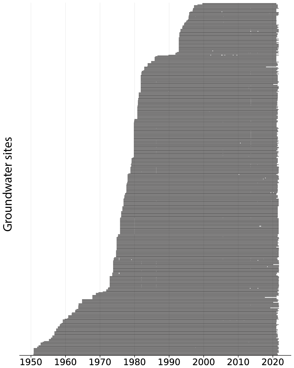
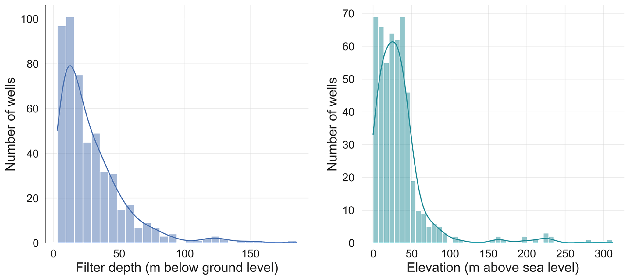
Figure A2 Filter depth (metres below ground level) and elevation (metres above sea level) of all the wells in the study area.

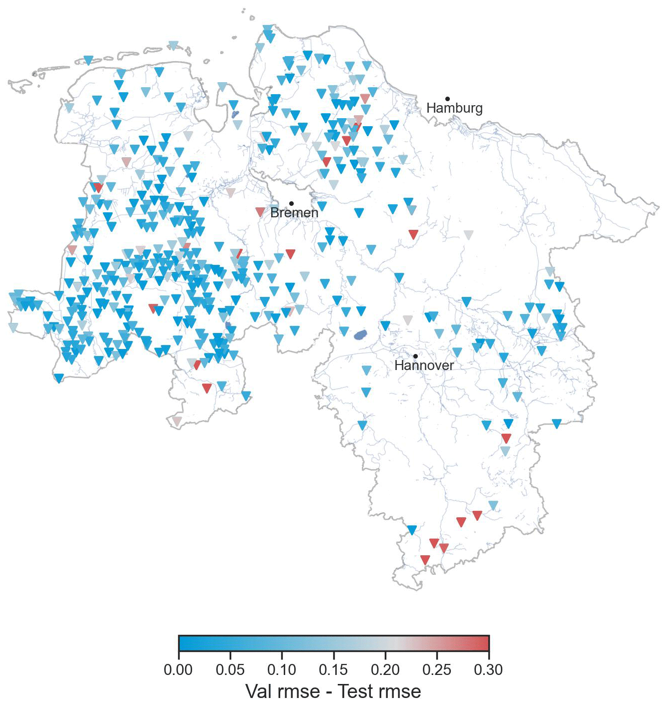
Figure A3 Difference in model performance (RMSE) between validation and testing periods.

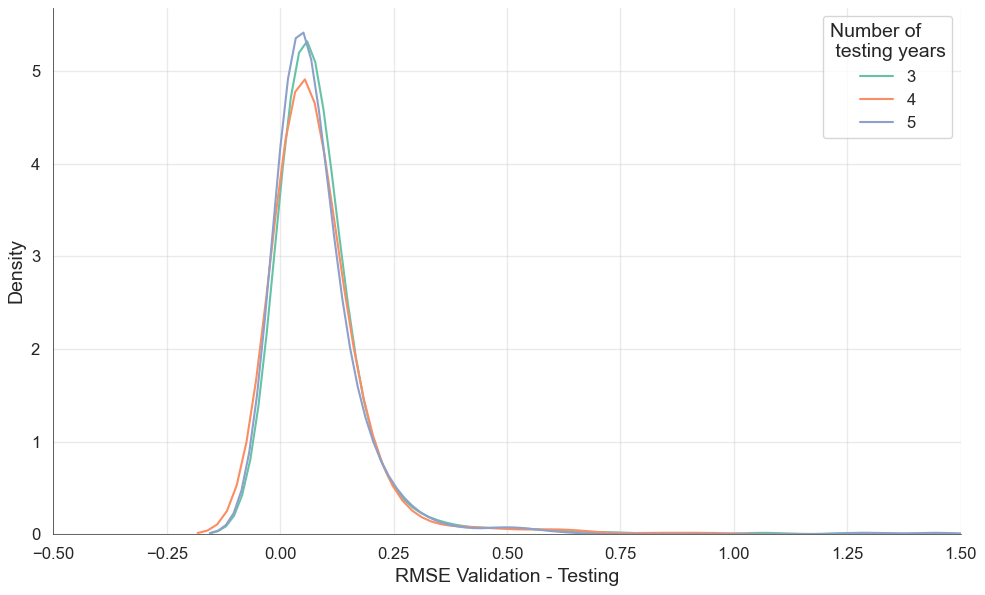
Figure A4 Model performance (RMSE) difference between validation and testing period for 3, 4, and 5 years of testing ranges.

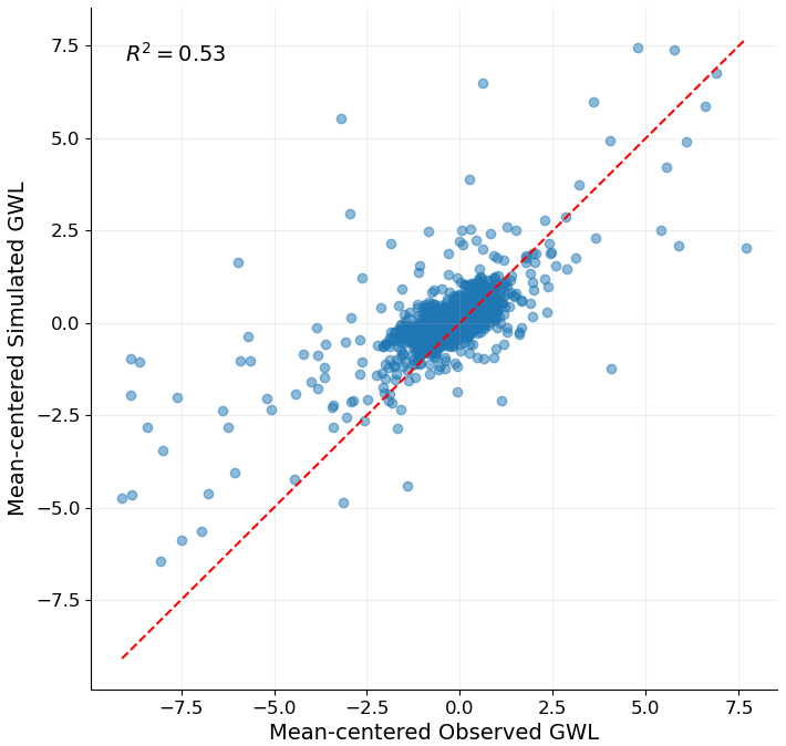
Figure A5 Scatterplot of simulated vs. observed values for the 505 wells for the test period.