Estimating the sensitivity of the Priestley–Taylor coefficient to air temperature and humidity

The Priestley–Taylor (PT) coefficient (α) is generally set as a constant value or is fitted as an empirical function of environmental variables, and it can bias the evaporation estimation or hydrological projections under global warming. By using an atmospheric boundary layer model, this study derives a theoretical and parameter-free equation for estimating α as a function of air temperature (T) and specific humidity (Q). With observations from several waterbodies and non-water-limited land sites, we demonstrate that, in addition to estimating the value of α well, the derived expressions can also capture the sensitivity of α to T and Q, that is, $\mathrm{d}\mathit{\alpha }/\mathrm{d}T$ and $\mathrm{d}\mathit{\alpha }/\mathrm{d}Q$. α is generally negatively associated with T and Q, in which regard T plays a more fundamental role in controlling α behaviors. Based on climate model data, we further show that this negative relationship between α and T is of great importance for long-term hydrological predictions. We also provide a lookup graph for practical and broad uses to directly find the values of $\mathrm{d}\mathit{\alpha }/\mathrm{d}T$ and $\mathrm{d}\mathit{\alpha }/\mathrm{d}Q$ under specific conditions. Overall, the derived expression gives a physically clear and straightforward approach to quantify changes in α, which is essential for PT-based hydrological simulation and projections.

1 Introduction

Evaporation from wet surfaces, including oceans, lakes, and reservoirs, is relevant to global hydrological cycles and water availability. There is a long history of developing theories and methods to estimate wet-surface evaporation (Bowen, 1926; Penman, 1948; Priestley and Taylor, 1972; Thornthwaite and Holzman, 1939; Yang and Roderick, 2019). Among the existing models, the Priestley–Taylor (PT) model or equation is known for its transparent structure and low input requirement (Priestley and Taylor, 1972). The PT equation is widely used in evaporation estimation across varied scales and is the basis for various hydrologic and land surface models. Specifically, the PT equation comes from the equilibrium evaporation (λE_eq), and λE_eq can be calculated as follows (Slatyer and McIlroy, 1961):

$$\begin{array}{}\text{(1)}& \mathit{\lambda }{E}_{\text{eq}}={\displaystyle \frac{{\mathit{\epsilon }}_{\mathrm{a}}}{{\mathit{\epsilon }}_{\mathrm{a}}+\mathrm{1}}}(R_n-G),\end{array}$$

where λ (J kg⁻¹) is the latent heat of water vaporization, ${\mathit{\epsilon }}_{\mathrm{a}}=\mathrm{\Delta }/\mathit{\gamma }$, Δ (kPa K⁻¹) is the slope of the saturated vapor pressure versus the temperature curve (a function of temperature), and γ is the psychrometric constant. ε_a is a function of air temperature (T). R_n−G (kPa K⁻¹) is the available energy. The equilibrium evaporation indicates that the near-surface air is saturated, supposing the vapor pressure deficit (VPD) is zero. However, it does not exist in the real world (Brutsaert and Stricker, 1979; Lhomme, 1997a) due to the continuous exchanges of warm and dry air from the entrainment layer, although water is continuously transported from the bottom wet surface into the atmosphere through the evaporation process (Fig. 1).

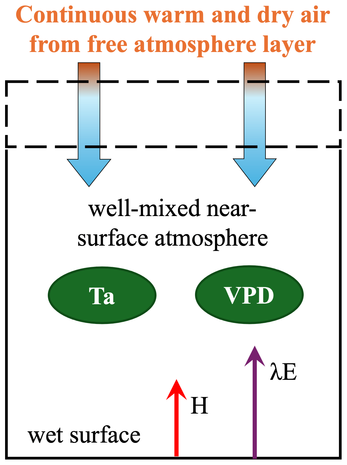
Figure 1 Atmospheric boundary layer box model describing the energy and water fluxes at the saturated surface and in the atmosphere above. The dotted line represents the removable upper boundary of the box. H and λE are the sensible and latent heat fluxes. Ta is the air temperature, and VPD is the vapor pressure deficit.

In this case, the PT equation introduced a parameter, α, known as the PT coefficient, to estimate wet-surface evaporation (Priestley and Taylor, 1972). α represents the effects of vertical mixing of dry and moist air and adjusts the equilibrium evaporation to the actual evaporation. So, qualitatively speaking, the α is impossibly lower than 1 because the air is always non-saturated and can only come infinitely close to a saturated condition, no matter how moist the near-surface air is. The PT equation is as follows:

$$\begin{array}{}\text{(2)}& \mathit{\lambda }E=\mathit{\alpha }{\displaystyle \frac{{\mathit{\epsilon }}_{\mathrm{a}}}{{\mathit{\epsilon }}_{\mathrm{a}}+\mathrm{1}}}(R_n-G).\end{array}$$

In the original study of Priestley and Taylor (1972), the value of α was fitted as 1.26. While a fixed α value can reasonably estimate wet-surface evaporation (Yang and Roderick, 2019), some studies found that α varies across time and space; for example, α often shows a more prominent value under cold conditions and becomes lower as temperature increases (Xiao et al., 2020; De Bruin and Keijman, 1979). This indicates that α should be a variable rather than a constant (Assouline et al., 2016; Guo et al., 2015; Jury and Tanner, 1975; Lhomme, 1997b; Van Heerwaarden et al., 2009; Eichinger et al., 1996; McNaughton and Spriggs, 1986; Crago et al., 2023; Maes et al., 2019). However, the hydrology field predominantly employs the fixed value of α=1.26 despite those earlier findings being over 3 decades old.

A general method to quantify the changes in α is to invert it with observations based on Eq. (2) and then build relationships among α and investigated variables. Since the existence of a negative relationship between α and temperature (T) is the consensus from multi-scale observations (Assouline et al., 2016; Xiao et al., 2020), many attempts empirically fitted α as a function of T (Andreas and Cash, 1996; Hicks and Hess, 1977; Yang and Roderick, 2019). Recent work further showed that the air humidity state can also influence the spatiotemporal patterns of α (Su and Singh, 2023). While those methods promote our understanding of the potential variations in α, they lie more on the empirical side and pay less attention to the underlying process. Hence, various endeavors have been made to calculate α through physical means, but they are often constrained by the complexity of numerous parameters. For instance, in the research conducted by Lhomme (1997b), α was explicitly formulated utilizing the PM model in conjunction with boundary layer theory. Nevertheless, the formulation incorporates parameters that signify surface and aerodynamic resistances, making them hard to determine through direct measurements. Subsequently, by using a refined boundary layer model, Van Heerwaarden et al. (2009) introduced a mathematical expression for estimating α; however, the expression also involves a set of parameters necessitating that numerical experiments delineate a feasible range for α. Consequently, obtaining a precise α estimation using conventional observations has still remained a challenge.

Based on a recent study by Liu and Yang (2021), here, we aim to derive a physically clear, transparent, and calibration-free equation for estimating α by introducing a governing equation (potential vapor pressure deficit budget) into the conventional boundary layer model. In the following sections, we will first provide the theory for estimating α and its sensitivity to climate conditions: air temperature (T) and humidity (represented by the air specific humidity, Q). We further evaluate the theory based on measurements from the water and non-water-limited land surfaces, followed by the influences of α changes over long-term hydrologic projections.

2 Theory

2.1 Derivation of the Bowen ratio

Here, we use a model based on the atmospheric boundary layer (ABL) as the basis for the Bowen ratio (Bo, defined as the ratio of sensible heat fluxes to latent heat fluxes, $H/\mathit{\lambda }E$) derivation (Liu and Yang, 2021). The fundamental conservation equations for states of moisture and energy over the water surfaces are as follows (Raupach, 2001):

$$\begin{array}{}\text{(3)}& {\displaystyle }\mathit{\rho }{c}_p{\displaystyle \frac{\mathrm{d}\mathit{\theta }}{\mathrm{d}t}}={\displaystyle \frac{H}{h}}+{\displaystyle \frac{\mathit{\rho }{c}_p{g}_{\mathrm{e}}}{h}}({\mathit{\theta }}_{\mathrm{e}}-\mathit{\theta }),\text{(4)}& {\displaystyle }\mathit{\rho }\mathit{\lambda }{\displaystyle \frac{\mathrm{d}Q}{\mathrm{d}t}}={\displaystyle \frac{\mathit{\lambda }E}{h}}+{\displaystyle \frac{\mathit{\rho }\mathit{\lambda }{g}_{\mathrm{e}}}{h}}(Q_{\mathrm{e}}-Q),\end{array}$$

where θ (K) is the potential temperature, Q is the specific humidity, c_p ($\mathrm{J}{\mathrm{kg}}^{-\mathrm{1}}{\mathrm{K}}^{-\mathrm{1}}$) is the specific heat capacity of air at constant pressure, g_e (m s⁻¹) is the entrainment flux velocity into the ABL box, and h (m) is the height of the ABL. The subscript e indicates that the variable is evaluated at the upper boundary of the ABL (see Fig. 1).

According to Eqs. (3) and (4), we can obtain a formula to calculate the rate of VPD ($\mathrm{d}\text{VPD}/\mathrm{d}t$; see details in Liu and Yang, 2021):

$$\begin{array}{}\text{(5)}& {\displaystyle \frac{\mathrm{d}\text{VPD}}{\mathrm{d}t}}={\displaystyle \frac{{\mathit{\epsilon }}_{\mathrm{a}}H-\mathit{\lambda }E}{\mathit{\rho }\mathit{\lambda }h}}+{\displaystyle \frac{g_{\mathrm{e}}}{h}}{\mathrm{\Delta }}_{\mathrm{D}},\end{array}$$

where Δ_D is calculated as

$$\begin{array}{}\text{(6)}& {\mathrm{\Delta }}_{\mathrm{D}}={\text{VPD}}_{\mathrm{e}}-\text{VPD}.\end{array}$$

Under the state in which the air is saturated, the water vapor is continuously transported from the water surface to the atmosphere, keeping the air saturated. In this case, there is no vertical moisture gradient; that is, the air near the surface and the air at the upper boundary of the ABL should be saturated, and so VPD and VPD_e are both equal to zero. With Eq. (6), we can know Δ_D=0.

When air is not saturated, we can rewrite Eq. (6) as follows:

$$\begin{array}{}\text{(7)}& {\mathrm{\Delta }}_{\mathrm{D}}=Q-Q_{\mathrm{e}}+\left[Q_{\text{sat}}\right({\mathit{\theta }}_{\mathrm{e}})-Q_{\text{sat}}(\mathit{\theta }\left)\right],\end{array}$$

where Q_e is much smaller than Q, and Q_sat(θ_e)−Q_sat(θ) is small (1 order of magnitude smaller than Q) so that the Δ_D roughly equals Q (Raupach, 2001; Liu and Yang, 2021).

Under a relatively long-term period (monthly and/or longer), there is a potential VPD budget $(\mathrm{d}\text{VPD}/\mathrm{d}t=\mathrm{0})$ over water surfaces (Raupach, 2001), and g_e can be estimated as the function of H and λE as follows:

$$\begin{array}{}\text{(8)}& g_{\mathrm{e}}={\displaystyle \frac{H+\mathrm{\Lambda }\cdot \mathit{\lambda }E}{\mathit{\rho }{c}_p{\mathit{\gamma }}_{\mathrm{v}}h}},\end{array}$$

where Λ is a constant (0.07), and γ_v is the potential virtual temperature gradient in the free atmosphere above the ABL. γ_vh can be set as a fixed value of 7 K (Liu and Yang, 2021). Combining Eqs. (5) and (8) with the VPD budget, we can obtain the expression for Bo:

$$\begin{array}{}\text{(9)}& \text{Bo}=\left\{\begin{array}{ll}{\displaystyle \frac{\mathrm{1}}{{\mathit{\epsilon }}_{\mathrm{a}}}}& \text{equilibrium},\\ {\displaystyle \frac{\mathrm{1}-\mathrm{\Lambda }\mathit{\chi }}{{\mathit{\epsilon }}_{\mathrm{a}}+\mathit{\chi }}}& \text{non-equilibrium},\end{array}\right.\end{array}$$

where $\mathit{\chi }=\frac{\mathit{\lambda }Q}{c_p{\mathit{\gamma }}_{\mathrm{v}}h}$, a function of Q.

2.2 Theoretical formula for α

The surface energy balance is expressed as follows:

$$\begin{array}{}\text{(10)}& R_n=H+\mathit{\lambda }E+G=(\mathrm{1}+\text{Bo})\mathit{\lambda }E+G.\end{array}$$

Combining Eqs. (2) and (10), α can be calculated as follows:

$$\begin{array}{}\text{(11)}& \mathit{\alpha }={\displaystyle \frac{\mathrm{1}}{\mathrm{1}+\text{Bo}}}{\displaystyle \frac{{\mathit{\epsilon }}_{\mathrm{a}}+\mathrm{1}}{{\mathit{\epsilon }}_{\mathrm{a}}}}.\end{array}$$

With Eqs. (9) and (11), we can derive the formula for α:

$$\begin{array}{}\text{(12)}& \mathit{\alpha }=\left\{\begin{array}{ll}\mathrm{1}& \text{equilibrium},\\ \mathrm{1}+{\displaystyle \frac{({\mathit{\epsilon }}_{\mathrm{a}}\mathrm{\Lambda }+\mathrm{1})\mathit{\chi }}{{\mathit{\epsilon }}_{\mathrm{a}}[{\mathit{\epsilon }}_{\mathrm{a}}+\mathrm{1}+(\mathrm{1}-\mathrm{\Lambda }\left)\mathit{\chi }\right]}}& \text{non-equilibrium}.\end{array}\right.\end{array}$$

Equation (12) is one of the main results in this study, and it can estimate α well compared to a large number of observations (Fig. 2; please see the description of observed data in Sect. 3).

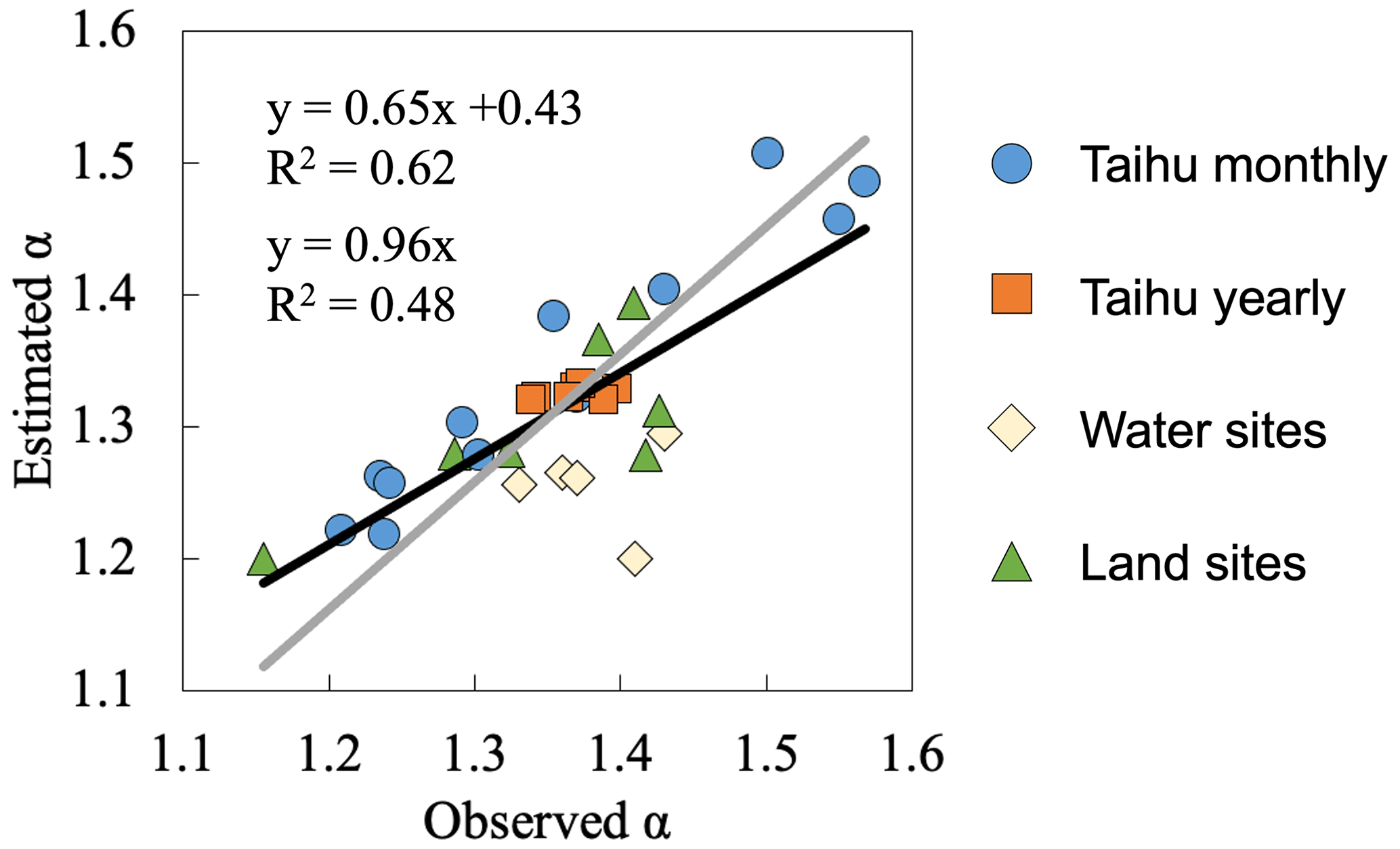
Figure 2 Comparison between observations and α calculated with Eq. (12). The black line is the linear fitting with intercept, and the gray line is the linear fitting through origin. The observed α is inversed by the PT model.

2.3 The sensitivity of α to air temperature and humidity

According to the above derivations, we can know that α is not a constant and that it changes with T and Q. The sensitivity of α to T and Q, $\mathrm{d}\mathit{\alpha }/\mathrm{d}T$ and $\mathrm{d}\mathit{\alpha }/\mathrm{d}Q$, determines the variation of α if the initial α value is given. In this section, we derive explicit equations to estimate $\mathrm{d}\mathit{\alpha }/\mathrm{d}T$ and $\mathrm{d}\mathit{\alpha }/\mathrm{d}Q$.

Firstly, we decompose α changes into those of T and Q with partial differential equations based on Eq. (11):

$$\begin{array}{}\text{(13)}& {\displaystyle }\begin{array}{rl}{\displaystyle \frac{\partial \mathit{\alpha }}{\partial T}}=& {\displaystyle }-{\displaystyle \frac{\mathrm{1}}{(\mathrm{1}+{\text{Bo}}_{\text{ABL}}{)}^{\mathrm{2}}}}{\displaystyle \frac{{\mathit{\epsilon }}_{\mathrm{a}}+\mathrm{1}}{{\mathit{\epsilon }}_{\mathrm{a}}}}{\displaystyle \frac{\partial {\text{Bo}}_{\text{ABL}}}{\partial T}}\\ {\displaystyle }& {\displaystyle }-{\displaystyle \frac{\mathrm{1}}{{\mathit{\epsilon }}_{\mathrm{a}}^{\mathrm{2}}}}{\displaystyle \frac{\mathrm{1}}{\mathrm{1}+{\text{Bo}}_{\text{ABL}}}}{\displaystyle \frac{\partial {\mathit{\epsilon }}_{\mathrm{a}}}{\partial T}},\end{array}\text{(14)}& {\displaystyle \frac{\partial \mathit{\alpha }}{\partial Q}}=-{\displaystyle \frac{\mathrm{1}}{(\mathrm{1}+{\text{Bo}}_{\text{ABL}}{)}^{\mathrm{2}}}}{\displaystyle \frac{{\mathit{\epsilon }}_{\mathrm{a}}+\mathrm{1}}{{\mathit{\epsilon }}_{\mathrm{a}}}}{\displaystyle \frac{\partial {\text{Bo}}_{\text{ABL}}}{\partial Q}},\end{array}$$

where partial differential terms of $\frac{\partial {\text{Bo}}_{\text{ABL}}}{\partial T}$ and $\frac{\partial {\text{Bo}}_{\text{ABL}}}{\partial Q}$ can be estimated based on Eq. (9) as

$$\begin{array}{}\text{(15)}& {\displaystyle \frac{\partial {\text{Bo}}_{\text{ABL}}}{\partial T}}=-{\displaystyle \frac{\mathrm{1}-\mathrm{\Lambda }\mathit{\chi }}{({\mathit{\epsilon }}_{\mathrm{a}}+\mathit{\chi }{)}^{\mathrm{2}}}}{\displaystyle \frac{\partial {\mathit{\epsilon }}_{\mathrm{a}}}{\partial T}},\text{(16)}& {\displaystyle \frac{\partial {\text{Bo}}_{\text{ABL}}}{\partial Q}}=-{\displaystyle \frac{\mathrm{\Lambda }{\mathit{\epsilon }}_{\mathrm{a}}+\mathrm{1}}{({\mathit{\epsilon }}_{\mathrm{a}}+\mathit{\chi }{)}^{\mathrm{2}}}}{\displaystyle \frac{\partial \mathit{\chi }}{\partial Q}},\end{array}$$

where terms of $\frac{\partial {\mathit{\epsilon }}_{\mathrm{a}}}{\partial T}$ and $\frac{\partial \mathit{\chi }}{\partial Q}$ can be approximated as

$$\begin{array}{}\text{(17)}& {\displaystyle \frac{\partial {\mathit{\epsilon }}_{\mathrm{a}}}{\partial T}}={\displaystyle \frac{\mathrm{1}}{\mathit{\gamma }}}{\displaystyle \frac{\partial \mathrm{\Delta }}{\partial T}},\text{(18)}& {\displaystyle \frac{\partial \mathit{\chi }}{\partial Q}}={\displaystyle \frac{\mathit{\lambda }}{c_p{\mathit{\gamma }}_{\mathrm{v}}h}},\end{array}$$

where Δ can be calculated as

$$\begin{array}{}\text{(19)}& \mathrm{\Delta }={\displaystyle \frac{\mathrm{4098}{e}_s}{(T+\mathrm{237.3}{)}^{\mathrm{2}}}}.\end{array}$$

Combining Eqs. (13)–(18), we can obtain the following:

$$\begin{array}{c}\text{(20)}& {\displaystyle \frac{\partial \mathit{\alpha }}{\partial T}}={\displaystyle \frac{\mathrm{1}}{\mathit{\gamma }}}\left[{\displaystyle \frac{\mathrm{1}}{(\mathrm{1}+{\text{Bo}}_{\text{ABL}}{)}^{\mathrm{2}}}}{\displaystyle \frac{\mathrm{1}-\mathrm{\Lambda }\mathit{\chi }}{({\mathit{\epsilon }}_{\mathrm{a}}+\mathit{\chi }{)}^{\mathrm{2}}}}{\displaystyle \frac{{\mathit{\epsilon }}_{\mathrm{a}}+\mathrm{1}}{{\mathit{\epsilon }}_{\mathrm{a}}}}-{\displaystyle \frac{\mathrm{1}}{{\mathit{\epsilon }}_{\mathrm{a}}^{\mathrm{2}}}}{\displaystyle \frac{\mathrm{1}}{\mathrm{1}+{\text{Bo}}_{\text{ABL}}}}\right]{\displaystyle \frac{\partial \mathrm{\Delta }}{\partial T}},\\ \text{(21)}& {\displaystyle \frac{\partial \mathit{\alpha }}{\partial Q}}={\displaystyle \frac{\mathrm{1}}{(\mathrm{1}+{\text{Bo}}_{\text{ABL}}{)}^{\mathrm{2}}}}{\displaystyle \frac{\mathrm{\Lambda }{\mathit{\epsilon }}_{\mathrm{a}}+\mathrm{1}}{({\mathit{\epsilon }}_{\mathrm{a}}+\mathit{\chi }{)}^{\mathrm{2}}}}{\displaystyle \frac{{\mathit{\epsilon }}_{\mathrm{a}}+\mathrm{1}}{{\mathit{\epsilon }}_{\mathrm{a}}}}{\displaystyle \frac{\mathit{\lambda }}{c_p{\mathit{\gamma }}_{\mathrm{v}}h}}.\end{array}$$

We can rewrite Eq. (20) as follows:

$$\begin{array}{}\text{(22)}& {\displaystyle \frac{\partial \mathit{\alpha }}{\partial T}}=-{\displaystyle \frac{\mathrm{1}}{\mathit{\gamma }}}{\displaystyle \frac{\mathit{\chi }\left[{\mathit{\epsilon }}_{\mathrm{a}}\right(\mathrm{\Lambda }{\mathit{\epsilon }}_{\mathrm{a}}+\mathrm{2})+\mathit{\chi }(\mathrm{1}-\mathrm{\Lambda })+\mathrm{1}]}{(\mathrm{1}+{\text{Bo}}_{\text{ABL}}{)}^{\mathrm{2}}({\mathit{\epsilon }}_{\mathrm{a}}+\mathit{\chi }{)}^{\mathrm{2}}{\mathit{\epsilon }}_{\mathrm{a}}^{\mathrm{2}}}}{\displaystyle \frac{\partial \mathrm{\Delta }}{\partial T}}.\end{array}$$

The total differentiation of α is

$$\begin{array}{}\text{(23)}& \mathrm{d}\mathit{\alpha }={\displaystyle \frac{\partial \mathit{\alpha }}{\partial T}}\mathrm{d}T+{\displaystyle \frac{\partial \mathit{\alpha }}{\partial Q}}\mathrm{d}Q.\end{array}$$

Thus, $\frac{\mathrm{d}\mathit{\alpha }}{\mathrm{d}T}$ and $\frac{\mathrm{d}\mathit{\alpha }}{\mathrm{d}Q}$ can be written as follows:

$$\begin{array}{}\text{(24)}& {\displaystyle \frac{\mathrm{d}\mathit{\alpha }}{\mathrm{d}T}}={\displaystyle \frac{\partial \mathit{\alpha }}{\partial T}}+{\displaystyle \frac{\partial \mathit{\alpha }}{\partial Q}}{\displaystyle \frac{\mathrm{d}Q}{\mathrm{d}T}},\text{(25)}& {\displaystyle \frac{\mathrm{d}\mathit{\alpha }}{\mathrm{d}Q}}={\displaystyle \frac{\partial \mathit{\alpha }}{\partial Q}}+{\displaystyle \frac{\partial \mathit{\alpha }}{\partial T}}{\displaystyle \frac{\mathrm{d}T}{\mathrm{d}Q}}.\end{array}$$

With the above equations, we can get theoretical relationships among α, T, and Q. This derivation can provide a simple and physically clear estimation for α changes. We also obtained $\mathrm{d}\mathit{\alpha }/\mathrm{d}T$ and $\mathrm{d}\mathit{\alpha }/\mathrm{d}Q$ values by fitting measured data using the linear regression model.

For practical use, we simplified Eqs. (20) and (21) as follows:

$$\begin{array}{}\text{(26)}& {\displaystyle \frac{\partial \mathit{\alpha }}{\partial T}}=-{\displaystyle \frac{\mathrm{1}}{\mathit{\gamma }}}{\displaystyle \frac{\mathit{\chi }}{{\mathit{\epsilon }}_{\mathrm{a}}+\mathit{\chi }}}{\displaystyle \frac{\mathrm{1}}{{\mathit{\epsilon }}_{\mathrm{a}}^{\mathrm{2}}}}{\displaystyle \frac{\partial \mathrm{\Delta }}{\partial T}},\text{(27)}& {\displaystyle \frac{\partial \mathit{\alpha }}{\partial Q}}={\displaystyle \frac{{\mathit{\epsilon }}_{\mathrm{a}}+\mathrm{1}}{{\mathit{\epsilon }}_{\mathrm{a}}({\mathit{\epsilon }}_{\mathrm{a}}+\mathit{\chi }+\mathrm{1}{)}^{\mathrm{2}}}}{\displaystyle \frac{\mathit{\chi }}{Q}}.\end{array}$$

We further gave a numerical plot to show how α changes with T and Q (Fig. 3). We plot this figure by setting $\mathrm{d}Q/\mathrm{d}T$ gradients from 0.0005, 0.0007, and 0.0009 K⁻¹ to ensure coverage of most of the cases over water surfaces. The lookup graphs in Fig. 3 can be used to directly find $\mathrm{d}\mathit{\alpha }/\mathrm{d}T$ and $\mathrm{d}\mathit{\alpha }/\mathrm{d}Q$ values. For example, for a water surface with $\mathrm{d}Q/\mathrm{d}T$ equating to about 0.0007 K⁻¹, the values of $\mathrm{d}\mathit{\alpha }/\mathrm{d}T$ and $\mathrm{d}\mathit{\alpha }/\mathrm{d}Q$ can be found in the second column of Fig. 3.

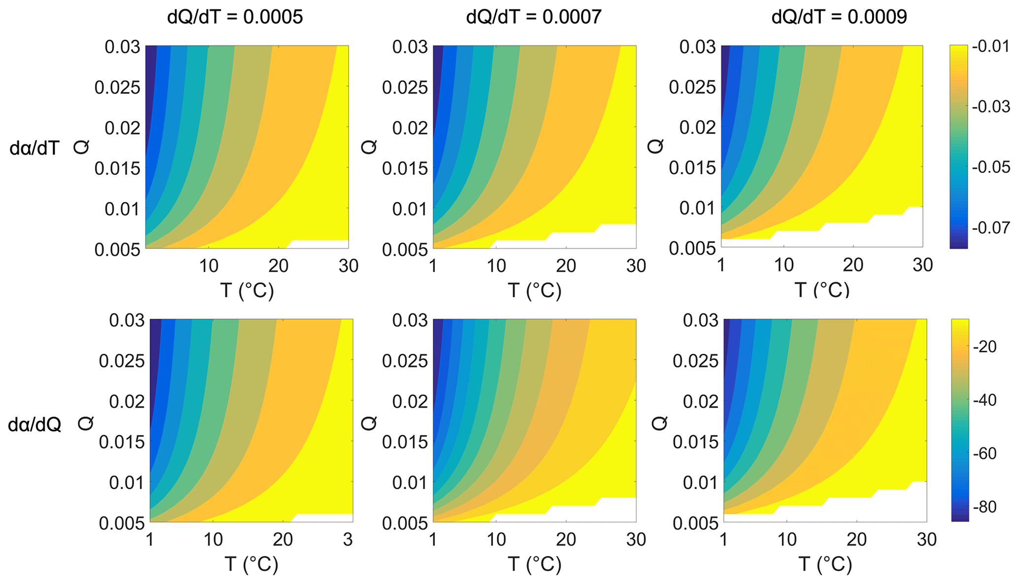
Figure 3 Values of $\mathrm{d}\mathit{\alpha }/\mathrm{d}T$ and $\mathrm{d}\mathit{\alpha }/\mathrm{d}Q$ under different T and Q. The first and second rows are $\mathrm{d}\mathit{\alpha }/\mathrm{d}T$ and $\mathrm{d}\mathit{\alpha }/\mathrm{d}Q$, respectively. The first to third columns are under different correlations between Q and T ($\mathrm{d}Q/\mathrm{d}T$) at 0.0005, 0.0007, and 0.0009 K⁻¹, respectively. The blank space in each subpanel refers to values of $\mathrm{d}\mathit{\alpha }/\mathrm{d}T$ and $\mathrm{d}\mathit{\alpha }/\mathrm{d}Q$ that are negative, indicating situations that rarely happen in the real world (i.e., with a very high temperature, the specific humidity is hardly deficient over wet surfaces).

3 Cases and applications

3.1 Data

We select data from eddy covariance measurements on several water surfaces (Han and Guo, 2023): (i) Lake Taihu, located in the Yangtze River Delta, China, with an area of ∼2400 km² and an average depth of 1.9 m (Lee et al., 2014) – there are five sites over the Taihu surface, and the poor-quality data marked with quality flags are removed; (ii) Lake Poyang, located in the Yangtze Plain, China, with an area of ∼3000 km² and an average depth of 8.4 m (Zhao and Liu, 2018); (iii) Erhai, located in the Yun-Gui Plateau of China, with an area of ∼250 km² and an average depth of 10 m (Du et al., 2018); (iv) the Guandu ponds, located in Anhui Province, China, with an area of ∼0.05 km² and an average depth of 0.8 m (Zhao et al., 2019); and (v) Lake Suwa, located in Nagano, Japan, with an area of ∼13 km² and an average depth of 4 m (Taoka et al., 2020). Months with negative values in terms of sensible heat fluxes have not remained. Given the absence of observed heat storage (G) at some sites, we use the sum of latent heat flux and sensible heat flux (i.e., LE+H) instead of net radiation minus G (R_n−G) as the measure of available energy. Using either LE+H or R_n−G yields identical results as our objective is to use the available energy to invert parameter α from observations. The latitude, longitude, and available data periods of the five lakes and ponds are listed in Table 1. For α changes in time, we use data from Lake Taihu for our investigation due to its sufficient data length. For α changes in space, we calculate the average temperature, specific humidity, and α of each lake for comparison.

Table 1 Location and date period of each waterbody.

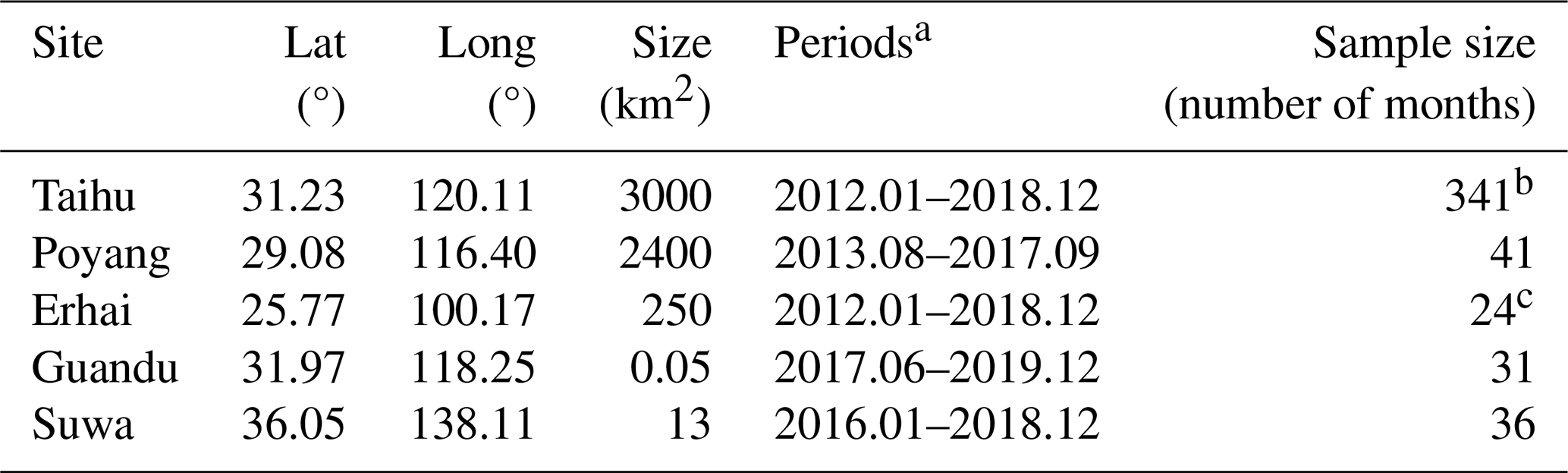
^a The term “periods” refers to the date of the first measurement to the date of the last one, including months for which no data are available. ^b There are five eddy covariance sites over Lake Taihu. ^c Only climatology monthly data from two periods of 2012–2015 and 2015–2018 are available.

Observations from global flux sites (FluxNet2015 database) are also selected. We first examine days without water stress based on the following steps (Maes et al., 2019). At each site, the evaporative fraction (i.e., EF, latent heat flux over the sum of latent and sensible fluxes) is first calculated, and the days with an EF exceeding the 95th-percentile EF and with an EF larger than 0.8 remain. Secondly, the days with soil moisture lower than 50 % of the maximum soil moisture (taken as the 98th percentile of the soil moisture series) are removed. Days having rainfall and negative values of latent and sensible heat fluxes are also not included. As a result, a total of ∼700 non-water-stressed site days meet the criteria. Data are divided into seven vegetation types, including croplands (CRO), wetlands (WET), evergreen needleleaf and mixed forests (DNF_MF), evergreen broadleaf and deciduous broadleaf forests (EBF_DBF), grasslands (GRA), close shrublands (CSH), and woody savanna (WSA), to analyze α changes in space. It should be noted that we do not average the daily data to a monthly scale due to variations in data sizes across different months for a specific site. Instead, we organize the selected daily data by vegetation type as the primary objective of utilizing land flux data is to assess the derived relationship spatially rather than temporally.

We also collect ocean surface data from 11 CMIP6 models (under scenario SSP585, Table 2) from 2021 to 2100 to see the temporal changes in α. The calculation is limited to the latitudinal range 60° S to 60° N and takes all ocean surface grids as a whole (Roderick et al., 2014). We average the monthly data to the yearly scale and calculate α every 10 years from 2021 to 2100 (i.e., 2021–2030, 2031–2040, etc.).

Table 2 CMIP6 models used in this study.

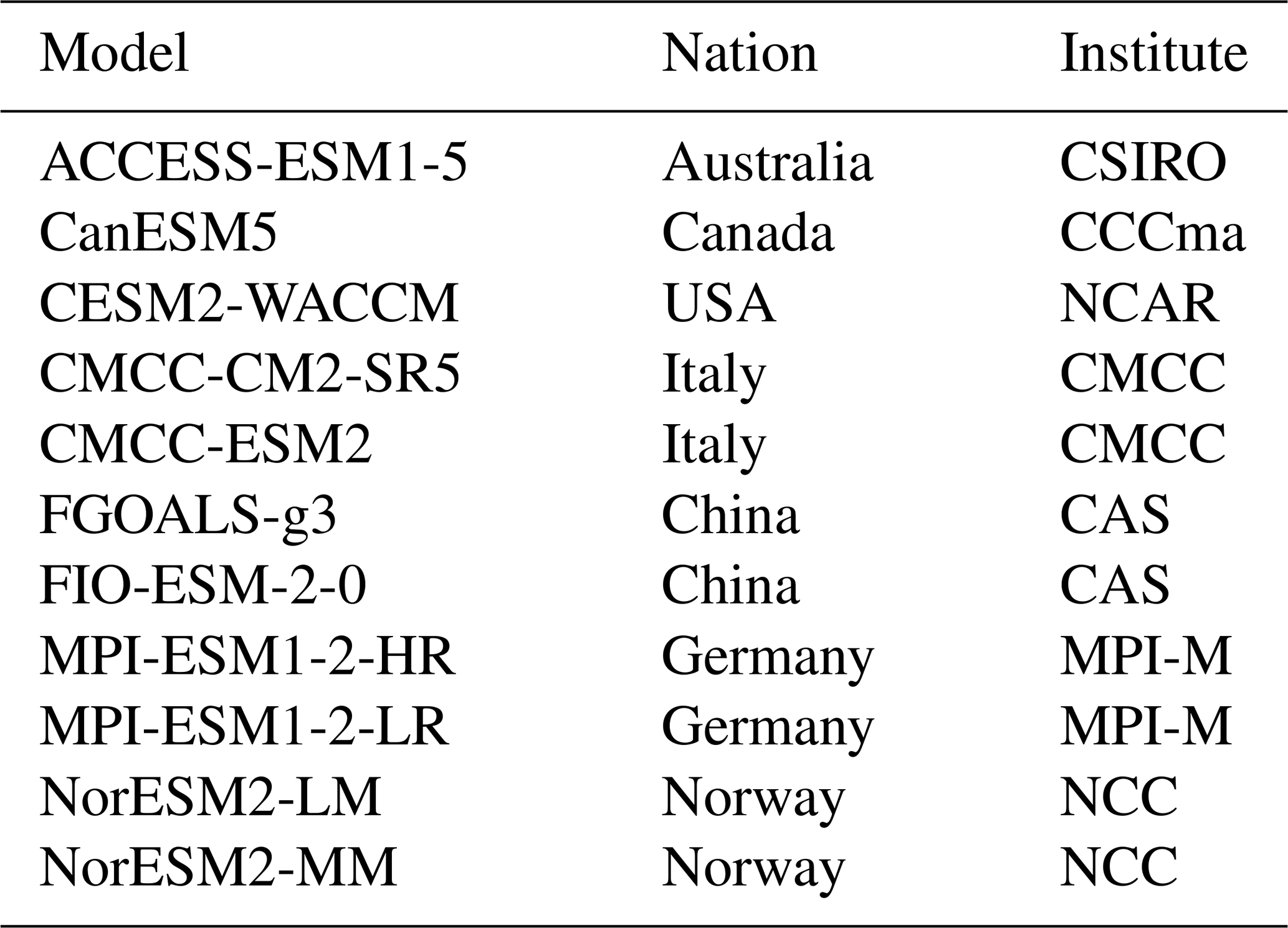
CSIRO is the Commonwealth Scientific and Industrial Research Organization, CCCma is the Canadian Centre for Climate Modelling and Analysis, NCAR is the National Center for Atmospheric Research, CMCC is the Euro-Mediterranean Center on Climate Change, CAS is the Chinese Academy of Sciences, MPI-M is the Max Planck Institute for Meteorology, and NCC is the Norwegian Climate Centre.

3.2 Results

3.2.1 Temporal and spatial changes in α

We used yearly and monthly (from January to December) climatology data from Lake Taihu to investigate the temporal variation in α. α is firstly inversed by the PT model and measurements, and then we found significant negative relationships of α with both T and Q (Fig. 4). On the yearly scale, the regressed values of $\mathrm{d}\mathit{\alpha }/\mathrm{d}T$ and $\mathrm{d}\mathit{\alpha }/\mathrm{d}Q$ are −0.029 °C⁻¹ and −47.42, and the values on the seasonal scale are −0.014 °C⁻¹ and −20.75, respectively. $\mathrm{d}\mathit{\alpha }/\mathrm{d}T$ on the seasonal scale is higher than that on the yearly scale because the variation range of α on the seasonal scale is more extensive. Theoretical derivations can roughly reproduce the sensitivity of α to T and Q, although there is some potential uncertainty from interannual variations (Table 3). We also analyzed the results on the 10 d scale and obtained similar findings (see Fig. A1 and Table A1 in the Appendix).

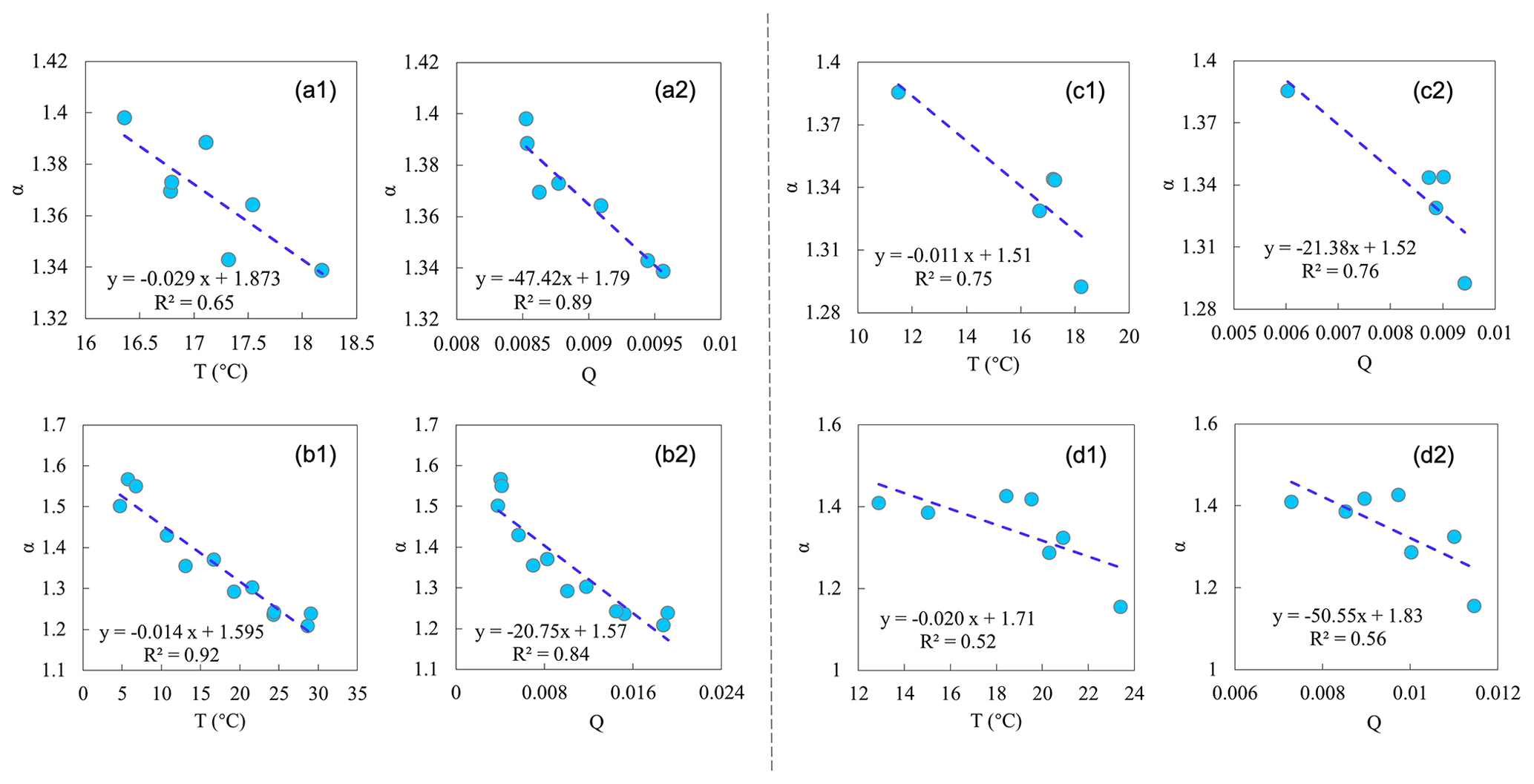
Figure 4 Temporal and spatial relationships of α and temperature (T) and specific humidity (Q). (a, b) Temporal relationships based on Lake Taihu data: (a) yearly data and (b) monthly climatology data. (c, d) Spatial relationships: (c) data from five water surface sites and (d) land surface data from FluxNet2015, with each circle representing one vegetation type. The linear regression line and correlation coefficient (R²) are shown in each subpanel.

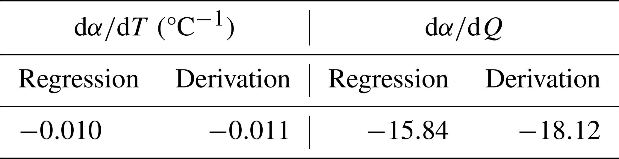
Table 3 Sensitivity of α to temperature (T) and specific humidity (Q) by regression and theoretical derivation.

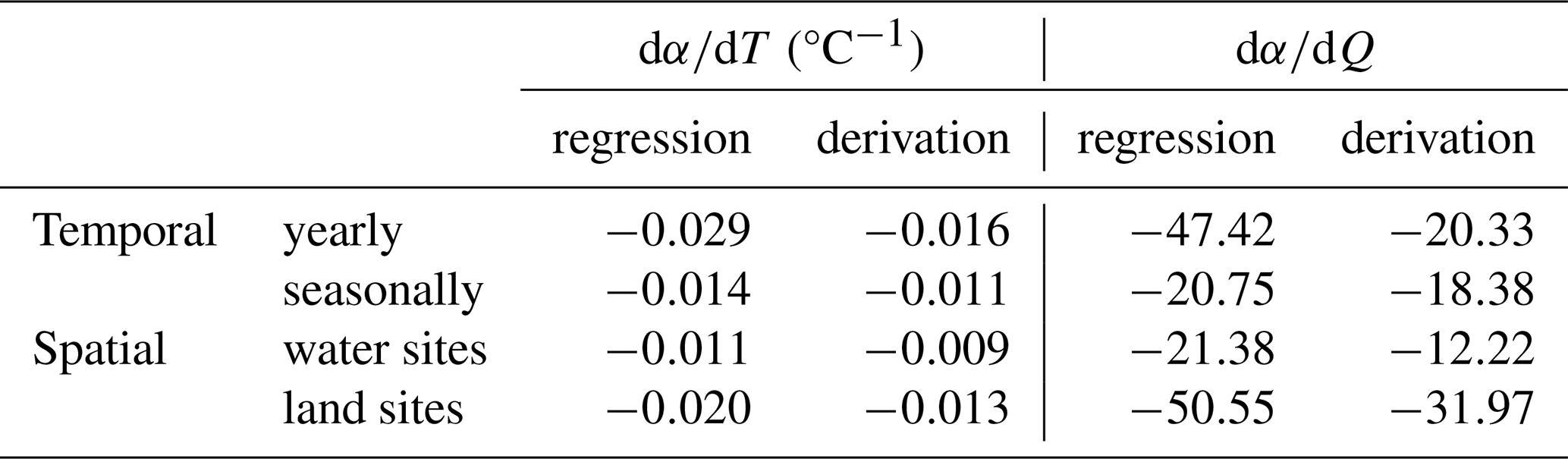
Spatial relationships of α with T and Q are similar to those in time; i.e., higher T and Q generally correspond to lower α, supported by measurements over both water and land surfaces (Fig. 4). For the water surfaces, the values of $\mathrm{d}\mathit{\alpha }/\mathrm{d}T$ and $\mathrm{d}\mathit{\alpha }/\mathrm{d}Q$ are −0.011 °C⁻¹ and −21.38, and the values for land surfaces are −0.020 °C⁻¹ and $-\mathrm{50.55}.$ The derived $\mathrm{d}\mathit{\alpha }/\mathrm{d}T$ and $\mathrm{d}\mathit{\alpha }/\mathrm{d}Q$ roughly matched well with the regressed values, despite more or fewer errors (Table 3). The correlations (represented by R² in Fig. 4) between α and T and between α and Q over water surfaces are higher than those over the land surfaces. This indicates that changes in α are more associated with T and Q over water surfaces, which may be because T and Q dominate the water surface evaporation process, while some other factors, like vegetation and wind speed, also play specific roles over land surfaces.

Based on Eqs. (20) to (22), $\partial \mathit{\alpha }/\partial T$ is always a negative value, and $\partial \mathit{\alpha }/\partial Q$ is always positive. The regressed and derived $\mathrm{d}\mathit{\alpha }/\mathrm{d}T$ and $\mathrm{d}\mathit{\alpha }/\mathrm{d}Q$ are both negative. Combined with Eqs. (24) and (25), considering the positive relationship between T and Q, the $\partial \mathit{\alpha }/\partial T$ plays a more critical role in determining (the signs of) $\mathrm{d}\mathit{\alpha }/\mathrm{d}T$ and $\mathrm{d}\mathit{\alpha }/\mathrm{d}Q$, that is, $|\partial \mathit{\alpha }/\partial T|>\partial \mathit{\alpha }/\partial Q\cdot \mathrm{d}Q/\mathrm{d}T$ and $|\partial \mathit{\alpha }/\partial T\cdot \mathrm{d}T/\mathrm{d}Q|>\partial \mathit{\alpha }/\partial Q$. Specifically, based on the data from Lake Taihu (for detecting α changes in time) and data from different water surface sites and land surface sites (for detecting α changes in space), we found the contribution of $\partial \mathit{\alpha }/\partial T\cdot \mathrm{d}T$ to dα is ∼70 %, which is much more significant than that of $\partial \mathit{\alpha }/\partial Q\cdot \mathrm{d}Q$ of ∼30 % (Table 4). Therefore, according to the evaporation process over the wet surface (Sect. 2.1) and the above analyses, we can conclude that α is fundamentally controlled by T and modulated by Q.

Table 4 Contributions of changes in temperature (T) and specific humidity (Q) to changes in α.

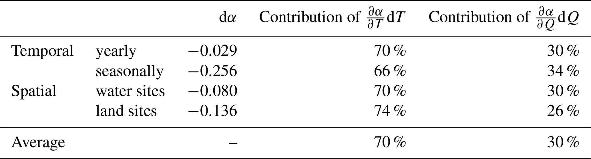
Note that, since $\mathrm{d}\mathit{\alpha }=\frac{\partial \mathit{\alpha }}{\partial T}\mathrm{d}T+\frac{\partial \mathit{\alpha }}{\partial Q}\mathrm{d}Q$, the contribution of $\frac{\partial \mathit{\alpha }}{\partial T}\mathrm{d}T$ is calculated as $\left|\frac{\partial \mathit{\alpha }}{\partial T}\mathrm{d}T\right|/\left|\frac{\partial \mathit{\alpha }}{\partial T}\mathrm{d}T+\frac{\partial \mathit{\alpha }}{\partial Q}\mathrm{d}Q\right|$, and the contribution of $\frac{\partial \mathit{\alpha }}{\partial Q}\mathrm{d}Q$ is calculated as $\left|\frac{\partial \mathit{\alpha }}{\partial Q}\mathrm{d}Q\right|/\left|\frac{\partial \mathit{\alpha }}{\partial T}\mathrm{d}T+\frac{\partial \mathit{\alpha }}{\partial Q}\mathrm{d}Q\right|$. dα refers to the estimated variation of α from the lowest to highest T (also from the lowest to highest Q since T and Q are generally positively correlated).

Derived $\mathrm{d}\mathit{\alpha }/\mathrm{d}T$ and $\mathrm{d}\mathit{\alpha }/\mathrm{d}Q$ have more or fewer errors compared to the regressed values. Several reasons can explain this: (i) there are errors in the measurements of eddy covariance systems; (ii) the additional factors other than T and Q, like wind speed, can also influence α; and (iii) the relationship of α and T (also of α and Q) cannot be well represented by the linear regression model. Besides, the water surface size effects on evaporation and α, reported by Han and Guo (2023), are not well considered in the presented derivation. Nevertheless, the derived expression can fairly match the observations of waterbodies with various sizes (Table 3).

3.2.2 Potential applications for global projections

Based on CMIP6 ocean surface data, we also detected significant negative relationships of α with T and Q (Fig. 5). $\mathrm{d}\mathit{\alpha }/\mathrm{d}T$ and $\mathrm{d}\mathit{\alpha }/\mathrm{d}Q$ obtained by the linear regression are −0.009 °C⁻¹ and −11.54, respectively. The derived $\mathrm{d}\mathit{\alpha }/\mathrm{d}T$ and $\mathrm{d}\mathit{\alpha }/\mathrm{d}Q$ are close to the regressed values at −0.009 °C⁻¹ and $-\mathrm{10.74}.$ We further compared the changes in T, Q, and heat fluxes between the first and the last 10 years in 2021–2100 (Table 5). To the end of this century, CMIP6 models predict that ocean average available energy (R_n−G) and latent heat fluxes (also evaporation) will increase by ∼3.1 and ∼6.0 W m⁻², respectively. Using the PT model with the fixed α (1.26), predicted evaporation shows an increase of ∼8.0 W m⁻², which is far higher than climate models' direct outputs (with a relative bias of ∼30 %). Based on derived α, ocean evaporation shows a much smaller increase of ∼5.8 W m⁻², with less than 5 % relative bias compared to CMIP6 values (Fig. 6). This indicates that changes in α should be well considered for the long-term projections. So, here, we suggest introducing the negative relationship between α and T, as proposed in this study, into the original PT model to correct for the overestimated sensitivity of evaporation to temperature (Liu et al., 2022), which could also improve the reliability of global long-term drought predictions (Greve et al., 2019).

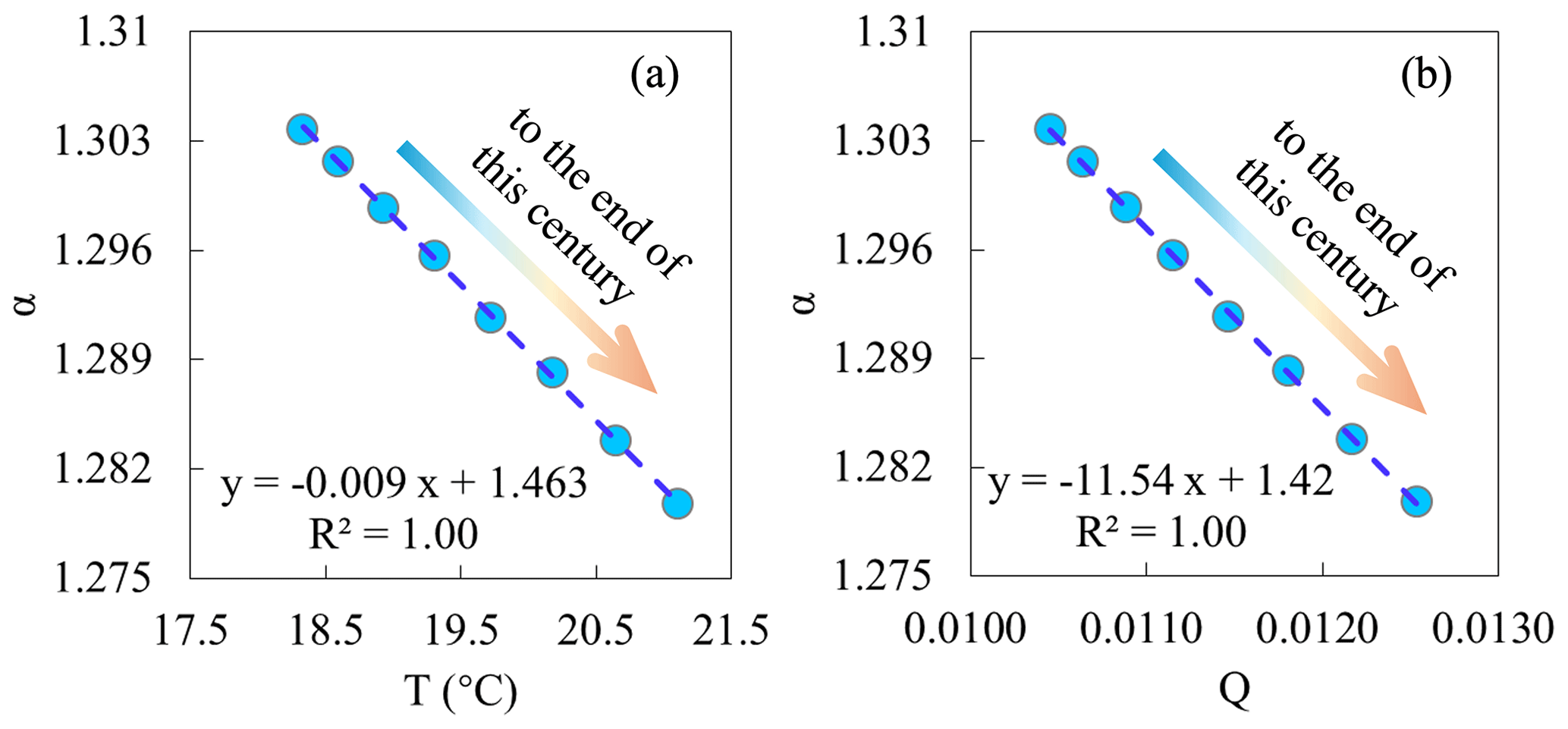
Figure 5 Temporal relationships of (a) α and temperature (T) and (b) α and specific humidity (Q) over global ocean surfaces. Each dot denotes the data in each 10-year window (2021–2030, 2031–2041, …, 2091–2100); from left to right is from 2021–2030 to 2091–2100.

Table 5 Ocean surface temperature, specific humidity, and heat fluxes for the first 10 years (2021–2030) and for the end of the 21st century (2091–2100). T, Q, R_n−G, and LE are direct outputs of climate models. α-CMIP refers to α inversed by the PT model with CMIP data. LE_PT is calculated by the PT model with fixed α at 1.26. α-ABL refers to α estimated by the ABL model. LE_ABL is calculated by the PT model with α-ABL.

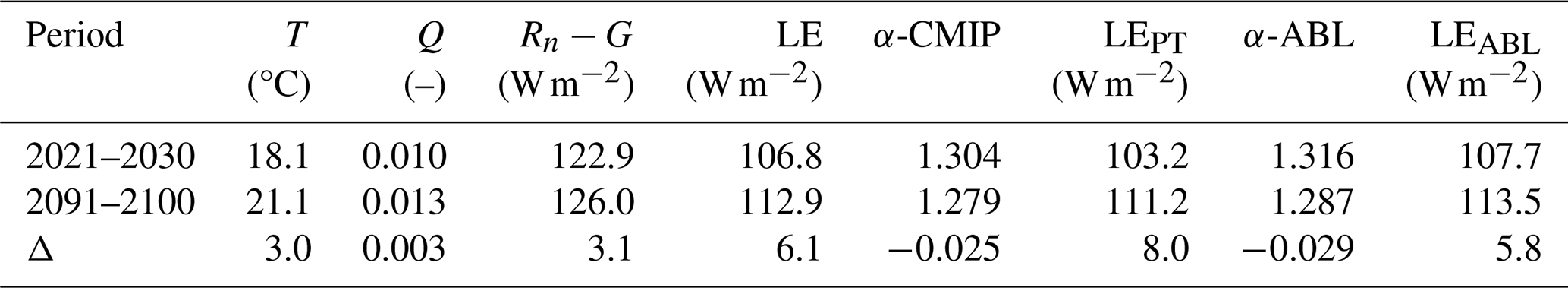
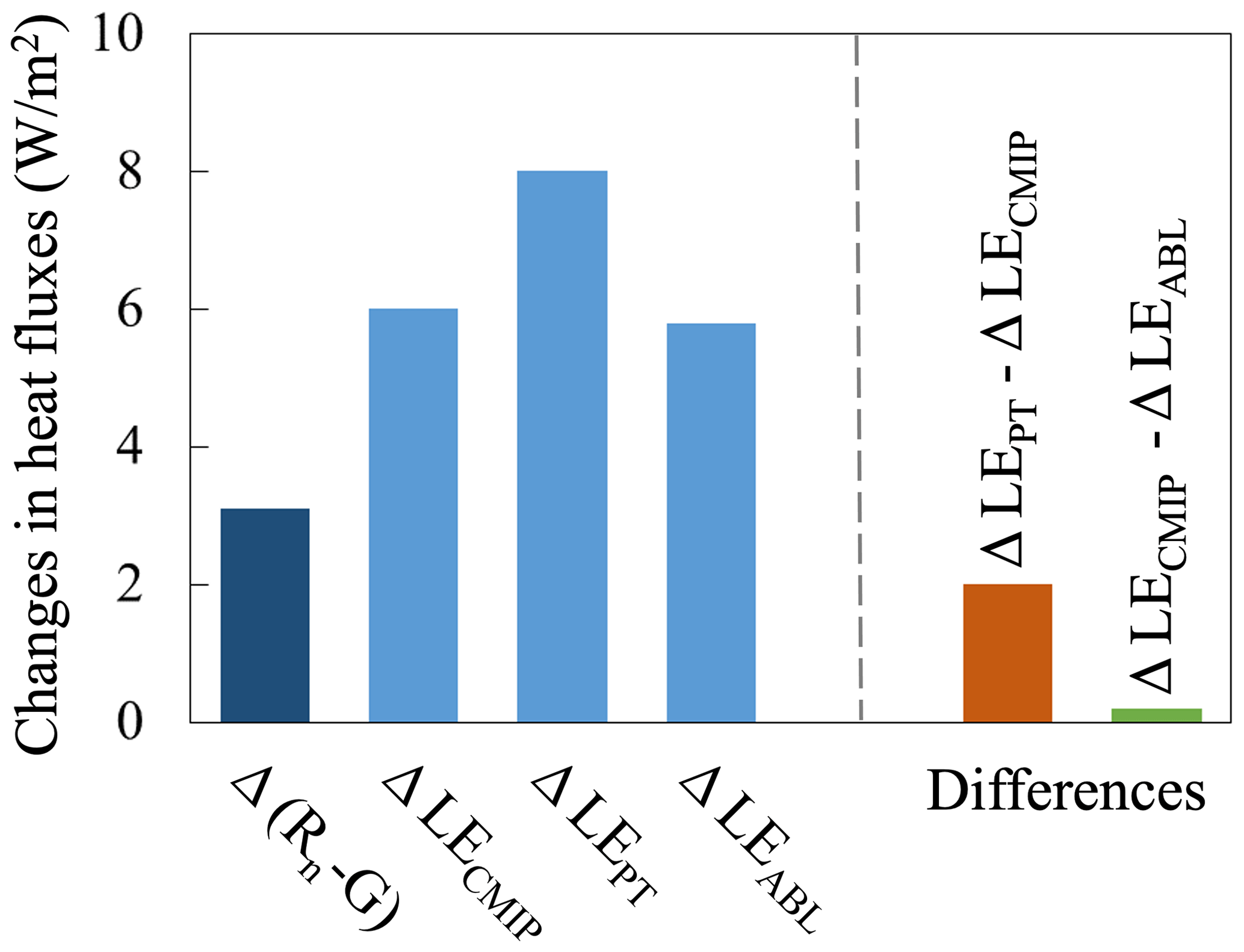
Figure 6 Stylized diagram showing the average changes in heat fluxes over global ocean surfaces.

4 Discussion and conclusions

In this study, we employed an open boundary layer model with a governing potential VPD budget (Raupach, 2001, 2000), originally integrated by Liu and Yang (2021), to formulate an expression for the Priestley–Taylor coefficient, α. Notably, the governing equation allows the derived expression to have no calibrated parameters and can estimate a precise α value with normal observations, rendering it superior to other methods that are also built with the boundary layer theory (Lhomme, 1997b; Van Heerwaarden et al., 2009). With the expression and a variety of measurements, we further demonstrated that temperature exerts a more significant influence over variations in α as opposed to specific humidity. We suggest that, for studies focusing on evaporation and/or drought projections, it is crucial to thoroughly characterize the negative correlation between α and temperature, a relationship easily determined using the derived expression.

It should be noted that, except for the PT model, the PM-based model can also be used to estimate wet-surface evaporation (Penman, 1948; Shuttleworth, 1993). While PM-based equations encapsulate all processes that possibly affect evaporation, the PT model, taking evaporation as a simple function of radiation and temperature, takes more account of the feedback and/or balance between the surface and near-atmosphere (Fig. 1). Besides, it has been noted that the PM-based models may fail at certain points and cannot capture the sensitivity of evaporation to temperature changes (Liu et al., 2022; McColl, 2020). So, in this case, also considering the fact that the PT model is currently one of the most popular equations due to its low input requirements, revisiting this classic model can greatly promote its adaption under the changing climate. Meanwhile, some revised PT equations can also be used to estimate the parameter α (Yang and Roderick, 2019; De Bruin and Holtslag, 1982). However, these modifications often exhibit significant deviations (Fig. A2). Specifically, the model developed by De Bruin and Holtslag (1982) is based on data from one specific site in the Netherlands, and the model built by Yang and Roderick (2019) comes from the fitness of global ocean surface data. These equations are primarily calibrated to match observed evaporation rates, while the underlying process is generally overlooked.

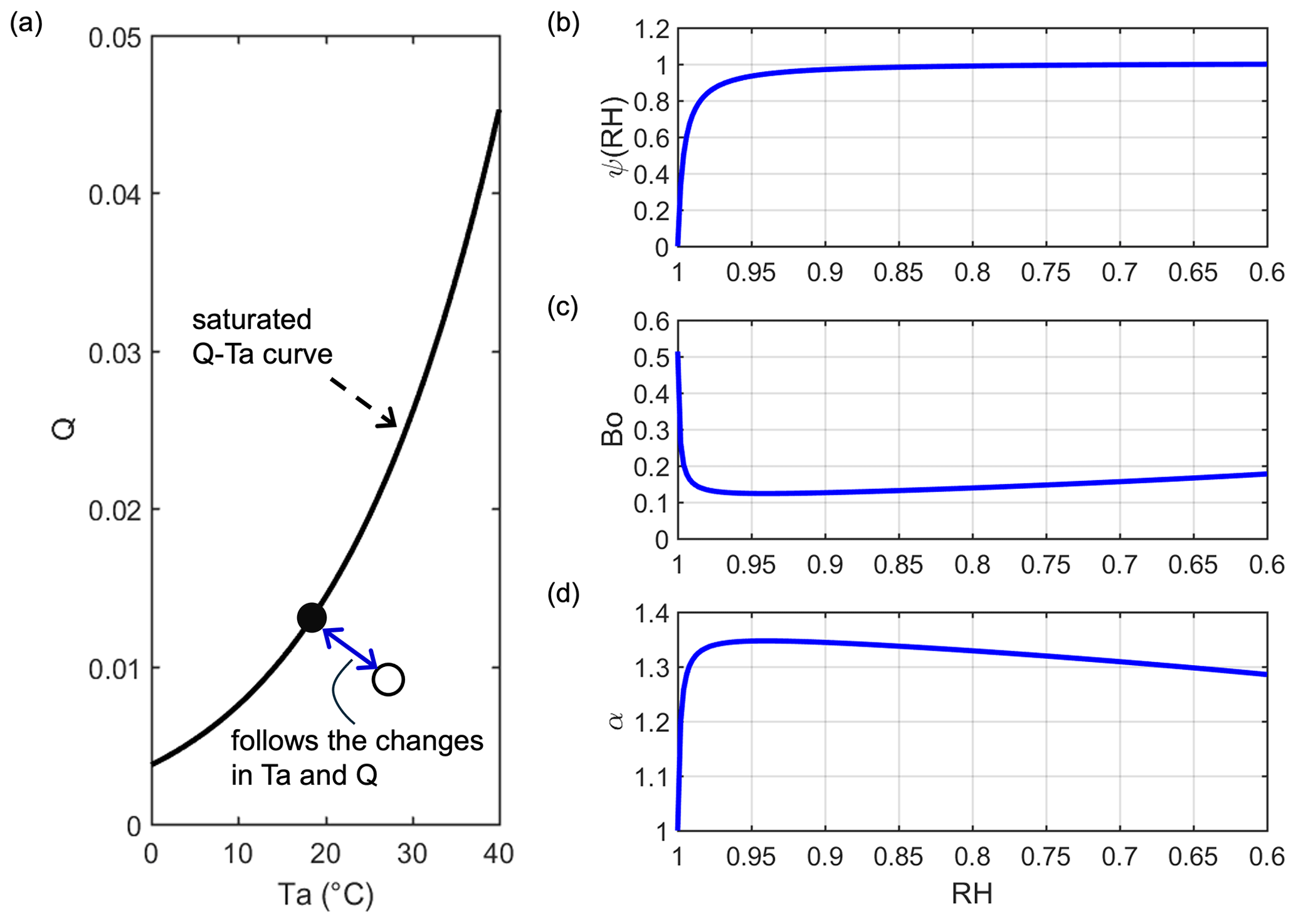
Figure 7 (a) Transition between saturated and non-saturated air states. The filled circle represents one case in which the air is saturated (saturated state), and the open circle represents one case in which air is not saturated (non-saturated state). (b) Relationship between ψ(RH) and RH with Eq. (28). (c, d) Changes in Bo and α as a function of RH when air temperature is fixed at 18 °C.

In Sect. 2.1, it was suggested that Δ_D=0 for the saturated air, while Δ_D≈Q for the non-saturated air. In theory, it is expected that the transition track between saturated and non-saturated states should be continuous and smooth. That is, the changes in the value of Δ_D between the saturated (0) and non-saturated (Q) states should follow the variations in air energy and moisture (Fig. 7). Since the relative humidity (RH) includes information on both air temperature and humidity, here, we introduce a possible track of Δ_D depending on RH as follows: ${\mathrm{\Delta }}_{\mathrm{D}}=\mathit{\psi }\left(\text{RH}\right)\cdot Q$. As we expect, the value of Δ_D approaches 0 when the air is very moist (i.e., very close to the saturated state and with RH close to 1), and so ψ should be a nonlinear and monotone convex function of RH. We give a possible expression of ψ(RH) as follows:

$$\begin{array}{}\text{(28)}& \mathit{\psi }\left(\text{RH}\right)=\mathrm{1}-{\displaystyle \frac{\mathrm{1}}{\mathrm{1}+m\times {\left(\frac{{\text{RH}}_{\text{max}}-\text{RH}}{\text{RH}-{\text{RH}}_{\text{min}}}\right)}^n}},\end{array}$$

where, over the water surfaces, RH_max is 1, and RH_min is 0.6 (McColl and Tang, 2023). m and n are shape parameters. To make ψ(RH) simple, we fixed n at 1 and let m be 100. The relationship between ψ(RH) and RH can be viewed in Fig. 7b. For a specific case with T at 18 °C, we show the changes in Bo and α with RH in Fig. 7c and d. Although there is a dramatic shift in Bo and α, this appears when RH is at 0.95–1, which is outside the vast majority of actual cases (RH is generally smaller than 0.9 on a monthly or longer scale). After the shift point, with RH decreases, ψ(RH), Bo, and α remain roughly stable. It is worth noting that Eq. (28) (with specific parameters) is one possible case that connects the transition between saturated and non-saturated air states, and a fine determination may be affected by local conditions, but a Δ_D value around Q is expected for most of the cases.

We recommend utilizing the derived model under warm conditions, for example, when the air temperature exceeds zero, to account for the prerequisite of a well-mixed boundary layer. In extremely cold regions or seasons, the water surface temperature can be lower than the air temperature, resulting in a downward sensible heat flux (De Bruin, 1982). Under such circumstances, the boundary layers exhibit relative stability and may not reach a well-mixed state. Additionally, we advise adopting a temporal scale ranging from weekly to monthly when applying the derived model. This is because the potential VPD budget (the governing equation) may not be rapidly achieved, such as on a diurnal or daily basis. Furthermore, over a longer term, the sensible heat flux typically manifests as upward in the majority of scenarios compared to a fine temporal scale.

The derived formula for α has important practical meanings. For example, it would be useful for estimating water surface evaporation and actual evapotranspiration based on the PT model (Miralles et al., 2011; Maes et al., 2019). It can also help to constrain the relationships among α, T, and Q in the complementary relationship, whose performance previously depended on the inversed α (Liu et al., 2016). Besides, considering the impacts of changing climate on α can significantly improve the performance of the hydrologic model in runoff simulations and predictions (Pimentel et al., 2023).

Appendix A

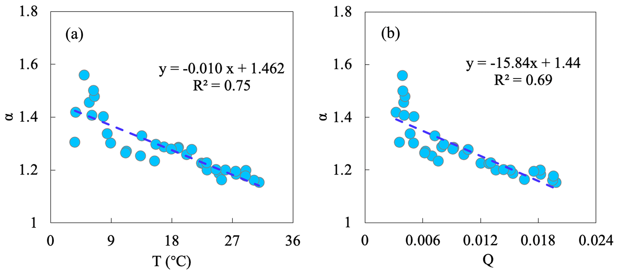
Figure A1 Relationships of α with (a) temperature (T) and with (b) specific humidity (Q) on the 10 d scale using water surface observations collected over Lake Taihu.

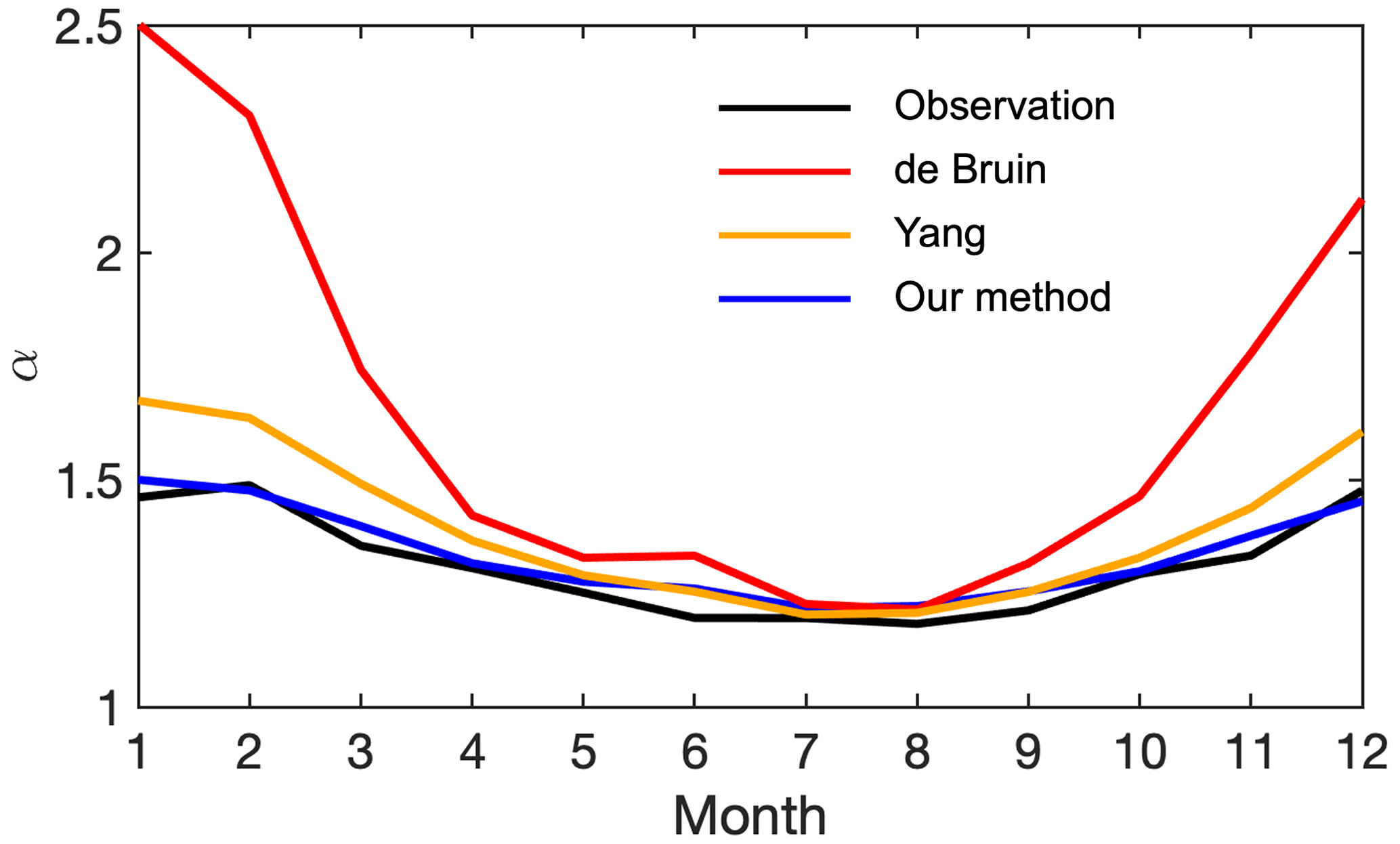
Figure A2 Observed (black) and estimated α over Lake Taihu. The blue line is α estimated with our method, and the red and orange lines are with two revised PT equations. The red line represents $\mathit{\alpha }=\mathrm{1}+\frac{\mathrm{20}}{\frac{\mathrm{\Delta }}{\mathrm{\Delta }+\mathit{\gamma }}(R_n-G)}$ (De Bruin and Holtslag, 1982), and the orange line represents $\mathit{\alpha }=\frac{\mathrm{\Delta }+\mathit{\gamma }}{\mathrm{\Delta }+\mathrm{0.24}\mathit{\gamma }}$ (Yang and Roderick, 2019).

Table A1 Sensitivity of α to temperature (T) and specific humidity (Q) on the 10 d scale.