Changes in mean evapotranspiration dominate groundwater recharge in semi-arid regions

Groundwater is one of the most essential natural resources and is affected by climate variability. However, our understanding of the effects of climate on groundwater recharge (R), particularly in dry regions, is limited. Future climate projections suggest changes in many statistical characteristics of the potential evapotranspiration (E_p) and the rainfall that dictate the R. To better understand the relationship between climate statistics and R, we separately considered changes to the mean, standard deviation, and extreme statistics of the E_p and the precipitation (P). We simulated the R under different climate conditions in multiple semi-arid and arid locations worldwide. Obviously, lower precipitation is expected to result in lower groundwater recharge and vice versa. However, the relationship between R and P is non-linear. Examining the ratio $R/P$ is useful for revealing the underlying relation between R and P; therefore, we focus on this ratio. We find that changes in the average E_p have the most significant impact on $R/P$. Interestingly, we find that changes in the extreme E_p statistics have much weaker effects on $R/P$ than changes in extreme P statistics. Contradictory results of previous studies and predictions of future groundwater recharge may be explained by the differences in the projected climate statistics.

1 Introduction

Groundwater sustainability depends on balancing groundwater recharge (R) and groundwater abstraction (Hartmann et al., 2017; Wada et al., 2010; Collenteur et al., 2021; Singh et al., 2019; De Filippi and Sappa, 2024; Viaroli et al., 2018; Andualem et al., 2021). R is the amount of water infiltrating the soil deep enough such that it is not lost to evaporation, transpiration, or runoff. Note that this definition is not the same as the definition of some authors, who define it as the amount of water replenishing the aquifer (Healy and Scanlon, 2010) (the main difference is the travel time). Many areas across the globe show a growing dependence on groundwater resources, which will only increase in the future (Bierkens and Wada, 2019; Taylor et al., 2013a, b). Climate variability affects both the precipitation and the evapotranspiration statistics. Therefore, understanding the potential effects of these factors on R is of great importance. In order to improve groundwater resource management and reduce negative human effects (Taylor et al., 2013a; Vivek et al., 2024; Pino-Vargas et al., 2023; Sappa et al., 2019; Quandt et al., 2023), the direct influences of climate variability on R must be quantified.

In recent years, much effort has been devoted to the analysis of the sensitivity of groundwater systems to climate change (Meixner et al., 2016; Pulido-Velazquez et al., 2015; Touhami et al., 2015; Fu et al., 2019; Döll and Fiedler, 2008; Tillman et al., 2016; Reinecke et al., 2021; Huang et al., 2023; Berghuijs, 2024; Berghuijs et al., 2024; Lorenzi et al., 2024; Langman et al., 2022). However, no conclusive generic outcomes can be drawn regarding the relationship between changes in climate conditions and the resulting changes in R rates (Al Atawneh et al., 2021; Green et al., 2011). The main source of uncertainties in future R are the uncertainties in climate predictions. It is unclear whether the climate variability is amplified or smoothed in the R response (Taylor et al., 2013a; Field et al., 2012; Reinecke et al., 2021; Moeck et al., 2016). Moreover, even the trend of the R response is uncertain (Smerdon, 2017).

Climate variability may also change the seasonal distribution of the precipitation (P) (Allan and Soden, 2008; Field et al., 2012). Increasing temperatures are expected to increase evapotranspiration (E_a) (Condon et al., 2020), while the increased CO₂ concentrations are expected to lower the E_a (Cao et al., 2010), and the overall effect is uncertain (Barnett et al., 2008). The future R uncertainties are even more dominant in arid and semi-arid regions, where the variability of the E_a affects the threshold values for R (Cuthbert et al., 2019b). Different studies have reached contradictory conclusions regarding the effects of climate change on R in arid and semi-arid regions (Crosbie et al., 2013). Some studies found that the changes in R are greater than the changes in climate conditions (Ng et al., 2010; McKenna and Sala, 2018), while others found a weak sensitivity of semi-arid regions to climate variability (Döll and Fiedler, 2008; Cuthbert et al., 2019a). Under future climate conditions, the precipitation and potential ET (E_p) statistics and, particularly, the frequency of extreme events (Myhre et al., 2019) may change. The effects of these extreme events may lead to an increase (Taylor et al., 2013b, a; Cuthbert et al., 2019b; Shamsudduha and Taylor, 2020; Goni et al., 2021) or a decrease (Cuthbert et al., 2019b) in R.

Previous studies investigated the R response to predicted future climate conditions using global climate models (GCMs) (Crosbie et al., 2013; Tillman et al., 2016) or regional GCM (Pulido-Velazquez et al., 2015) predictions. Pulido-Velazquez et al. (2015) also considered modifications of the mean and standard deviation (SD) of the P in the regional GCM predictions. However, these studies could not provide a conclusive understanding of the effects; in particular, changes in the E_p statistics were not directly considered.

The main objective of this study is to explore the changes in diffuse (rather than focused, agricultural, or mountain; see Meixner et al., 2016) R in semi-arid and arid regions due to changes in P and E_p statistics. In areas where R occurs predominantly through focused processes, additional factors dominate the overall recharge and are beyond the scope of this study. Here, R is defined as the accumulated water flux at a 5 m depth, assuming that this flux reaches the water table. To enhance our understanding of the R response to climate variability, we separately consider the changes in the (1) mean, (2) SD, and (3) extreme events of E_p and P statistics (relative to the measured statistics) in multiple locations across the globe. While we do not consider specific future climate projections, we identify and quantify the effects of changes in climate variable statistics on R in semi-arid and arid regions.

2 Methods

Groundwater recharge is a fraction of precipitation. Within the linear response regime, changes in precipitation would lead to a change in the recharge but not a change in the ratio between the groundwater recharge and the precipitation. To emphasize the non-linear response, we present the ratio between the recharge and the precipitation and the changes in these ratios. We use a numerical model to simulate the R under atmospheric boundary conditions. In what follows, we provide the details of the model, the independent data used for verification of the model, and the changes applied to the climate variable statistics.

2.1 Groundwater recharge data and modeling

To explore the impact of climate statistics on R, we identified 196 semi-arid and arid locations (see the Supplement) in which R was estimated using ground-based methods such as chloride mass balance, water isotopes, etc. (Taylor et al., 2013b; Scanlon et al., 2006; Moeck et al., 2020). These locations span both hemispheres and different continents (see Fig. 1a). Furthermore, they cover a wide range of soil types (Fig. 1b) and climate conditions, including various seasonal P distributions relative to temperature and other factors affecting evapotranspiration. The locations are characterized by bare soil or sparse vegetation, where transpiration is negligible relative to the evaporation. For locations where the model did not perform well, factors such as land use change may explain the discrepancies between simulated and reported R. In some locations, over the last decades, R may have changed substantially due to various human modifications of landscapes, such as changes in land use and land cover, as well as water conservation works (Turkeltaub et al., 2018; Favreau et al., 2009; Allison et al., 1990). Since the R fluxes estimated by the ground-based methods represent an integration over varying timescales, they are likely to reflect different stages of this evolution.

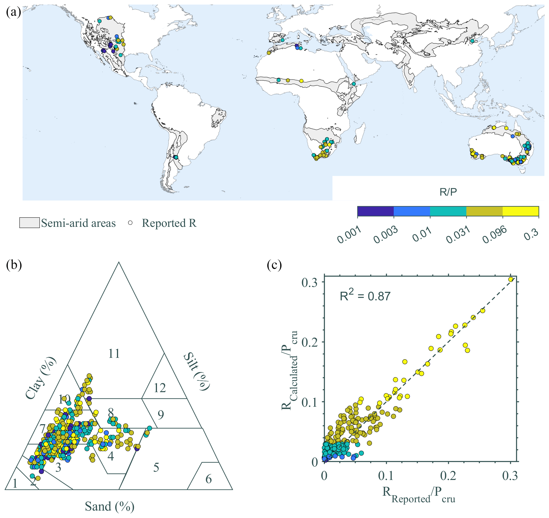
Figure 1 (a) The geographic distribution of the locations considered. (b) The soil composition, in terms of sand, silt, and clay, for all the locations considered in this study. The data are based on Hengl et al. (2014) and represent the reported soil characteristics for 0–5, 5–15, and 15–30 cm depths. (c) The simulated and reported ratio between the precipitation and the groundwater recharge for all the locations (in addition to the R² provided in the plot, other statistical indices for model performance evaluation are also provided: $\text{mean error}=-\mathrm{0.0058}$; mean absolute error=0.016; root mean square error=0.02).

Diffuse R fluxes were simulated using unsaturated flow modeling for these locations by numerically solving the 1D vertical Richards equation:

$$\begin{array}{}\text{(1)}& {\displaystyle \frac{\partial \mathit{\theta }}{\partial t}}={\displaystyle \frac{\partial }{\partial z}}\left[K\left(\mathit{\psi }\right)\left({\displaystyle \frac{\partial \mathit{\psi }}{\partial z}}+\mathrm{1}\right)\right],\end{array}$$

where ψ is the matric potential head (L), θ is the volumetric water content (dimensionless), t is time (T), z is the vertical coordinate (L), and K(ψ) (L T⁻¹) is the unsaturated hydraulic conductivity function. The Richards equation was numerically integrated using the Hydrus 1D (Šimŭnek et al., 2009). Knowledge regarding the soil hydraulic functions is essential in order to solve the Richards equation. The soil retention curves and the unsaturated hydraulic curves are commonly described according to the van Genuchten–Mualem (VGM) model (Mualem, 1976; Van Genuchten, 1980):

$$\begin{array}{}\text{(2)}& S_{\mathrm{e}}={\displaystyle \frac{\mathit{\theta }-{\mathit{\theta }}_{\mathrm{r}}}{{\mathit{\theta }}_{\mathrm{s}}-{\mathit{\theta }}_{\mathrm{r}}}}={\left[\mathrm{1}+{\left(\mathit{\alpha }\left|\mathit{\psi }\right|\right)}^n\right]}^{-m},\end{array}$$

where S_e is the degree of saturation ($\mathrm{0}<S_{\mathrm{e}}<\mathrm{1}$); θ_s and θ_r are the saturated and residual volumetric soil water contents, respectively; and α (L⁻¹), n, and $m=(\mathrm{1}-\mathrm{1}/n)$ are shape parameters. Hydraulic conductivity is assumed to behave according to the following:

$$\begin{array}{}\text{(3)}& K\left(S_{\mathrm{e}}\right)=K_{\mathrm{s}}{S}_{\mathrm{e}}^l{\left[\mathrm{1}-[\mathrm{1}-S_{\mathrm{e}}^{\mathrm{1}/m}{]}^m\right]}^{\mathrm{2}},\end{array}$$

where K_s (L T⁻¹) is the saturated hydraulic conductivity, and l is the pore connectivity parameter prescribed as 0.5.

Assuming that the unsaturated zone mainly consists of siliciclastic materials, the VGM parameters were determined using the pedo-transfer function ROSETTA (Zhang and Schaap, 2017), which uses a neural network to estimate the soil hydraulic parameters from soil attributes, such as soil texture and bulk density. Sand, silt, and clay contents and the bulk density were extracted at the considered locations from global soil maps reported by Hengl et al. (2014). Note that the data are divided into seven layers, but for the current study, only information from the top three layers was used (0–5, 5–15, and 15–30 cm; the VGM parameters are provided in the Supplement). We assume that evaporation is mostly limited to the topsoil (Or et al., 2013); therefore, we only considered the heterogeneity of these levels. Furthermore, the water table depths at the investigated locations, which were extracted from the global map presented by Fan et al. (2013), indicated that, in most locations, groundwater is below 0.8 m depth, and no phreatic evaporation is expected (see the Supplement; Chengcheng et al., 2020; Hellwig, 1973).

The water flow simulations were carried out using atmospheric-boundary conditions with surface runoff. Daily precipitation and E_p (potential ET) values were specified at the upper boundary. The minimum allowed pressure head at the soil surface was constant (hCritA=100 000 cm). Lower-boundary conditions were prescribed as free drainage, where the water flux across this boundary is considered to be the R. The depth of the simulated soil column was 500 cm, and it was discretized into 101 grid cells. A finer node spacing was implemented at the upper boundary, where the top node was 3 times thinner than the bottom node. Water content at field capacity was prescribed as the initial condition at the start of each simulation. Each simulation was run for 146 100 d, and the calculated daily R fluxes between days 73 050 and 146 100 were used for the analyses to avoid the influence of the initial conditions. In all the locations considered, the differences between the estimated and the reported $R/P$ ratios were below 5 %, illustrating the suitability of the model.

2.2 Climate data and generation of P and E_p time series

The CRU TS 3.2 climate dataset (Harris et al., 2014), including daily values of precipitation and potential evapotranspiration (E_p), was used for the analyses presented in the current study. The datasets were temporally downscaled, following van Beek (2008), to daily values using ERA40 (1958–1978, Uppala et al., 2005) and ERA-Interim (1979–2015, Dee et al., 2011). The daily E_p values were calculated according to the Penman–Monteith method using climate variables such as mean, maximum, and minimum temperatures; vapor pressure; cloud cover; and wind speed (Harris et al., 2014). Stochastic P and E_p time series spanning 400 years (146 100 d) were synthesized based on these 58 year-long CRU TS 3.2 records of daily precipitation and potential evapotranspiration (E_p). P time series were established based on the empirical histograms of the number of rainy days and the daily P amount distributions (see the Supplement; Turkeltaub and Bel, 2023). The E_p time series were established by random sampling of E_p empirical distributions for each calendar month separately (Turkeltaub and Bel, 2023). Furthermore, it was shown by the authors (Turkeltaub and Bel, 2023) that the best synthesis method involves a correction of the synthesized climate to match the observed monthly statistics. Thus, the P and E_p time series were corrected accordingly (see the examples in Figs. S1 and S2 in the Supplement for the effects of the correction on the monthly P and E_p statistics).

2.3 Modification of the mean (μ) and the standard deviation (SD, σ)

To examine the effects of changes in the statistics of the P and the E_p time series on groundwater recharge (R), the yearly mean, μ, and SD, σ, of these series were modified. Note that, when we modify the average of a time series, the SD is conserved and vice versa. The modification of μ is simply conducted by adding to each value (in the P series, only to non-zero values) in the original time series the difference between the original and modified yearly average divided by the number of relevant days in that year. Note that this correction could possibly have resulted in negative daily P and E_p amounts when considering a reduction in the yearly averages. Therefore, for the E_p, only days with amounts above the correction were modified in order to ensure non-negative values of E_p for all days. For the P series, we further wanted to conserve the statistics of the number of rainy days. Therefore, the maximal allowed reduction in P sets the value to 1 mm d⁻¹ (Turkeltaub and Bel, 2023). The modification of the SD is done in two stages. Firstly, each value in the original time series is multiplied by the ratio between the original SD, σ_org, of the total yearly P or the E_p and the modified SD, σ_mf. Subsequently, the differences between the averages of the original and the modified time series are corrected according to the procedure described above to preserve the original mean. Mathematically, the correction method for the annual μ of a time series is described as follows:

$$\begin{array}{}\text{(4)}& \text{MTS}{}_{\mathit{\mu }}\left(t\right)=\left\{\begin{array}{ll}\text{OTS}\left(t\right)\ge \text{threshold}& \text{OTS}\left(t\right)+{\displaystyle \frac{\mathrm{\Delta }}{\text{Na}\left(t\right)}}\\ \text{OTS}\left(t\right)<\text{threshold}& \text{OTS}\left(t\right)\end{array}\right.,\end{array}$$

where MTS_μ and OTS are the modified mean and the original time series, respectively. Δ is the difference between the modified and the original annual P or E_p averages ($\mathrm{\Delta }\equiv \langle {\text{MTS}}_{\mathit{\mu }}{\rangle }_{\mathrm{a}}-\langle \text{OTS}{\rangle }_{\mathrm{a}}$, and 〈.〉_a is the annual average of the variable represented in the time series). Na(t) is the number of days in the year of time t with P or E_p values larger than the threshold. The threshold is defined as $-\mathrm{\Delta }/\text{Na}\left(t\right)$ for the E_p and as $-(\mathrm{\Delta }/\text{Na}(t)+\mathrm{1})$ for the P. Na(t) is found recursively.

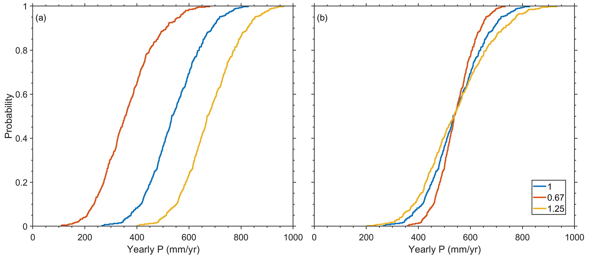
Figure 2 An example for the modification of the (a) mean, μ, and (b) the SD, σ, of a P time series for a specific location where a groundwater recharge flux was reported (145.711, −36.4469; Crosbie et al., 2010). The different colors correspond to the indicated modification factors.

To modify the σ of a time series, the following transformation is applied:

$$\begin{array}{}\text{(5)}& {\displaystyle }\begin{array}{rl}{\displaystyle }& {\displaystyle }{\mathrm{\text{MTS}}}_{\mathit{\sigma }}\left(t\right)=\\ {\displaystyle }& {\displaystyle }\left\{\begin{array}{ll}\text{OTS}\left(t\right)\times {\displaystyle \frac{{\mathit{\sigma }}_{\mathrm{m}}}{{\mathit{\sigma }}_{\mathrm{o}}}}\ge \text{threshold}& \text{OTS}\left(t\right)\times {\displaystyle \frac{{\mathit{\sigma }}_{\mathrm{m}}}{{\mathit{\sigma }}_{\mathrm{o}}}}+{\displaystyle \frac{{\mathrm{\Delta }}_{\mathit{\sigma }}}{\text{Na}\left(t\right)}}\\ \text{OTS}\left(t\right)\times {\displaystyle \frac{{\mathit{\sigma }}_{\mathrm{m}}}{{\mathit{\sigma }}_{\mathrm{o}}}}<\text{threshold}& \text{OTS}\left(t\right)\times {\displaystyle \frac{{\mathit{\sigma }}_{\mathrm{m}}}{{\mathit{\sigma }}_{\mathrm{o}}}}\end{array}\right.,\end{array}\end{array}$$

where σ_m and σ_o are the modified and original yearly standard deviation of the time series, respectively. ${\mathrm{\Delta }}_{\mathit{\sigma }}\equiv \langle \text{OTS}{\rangle }_{\mathrm{a}}(\frac{{\mathit{\sigma }}_{\mathrm{m}}}{{\mathit{\sigma }}_{\mathrm{o}}}-\mathrm{1})$. The threshold is defined similarly to the definition above for the mean modification. Figure 2 depicts an example of the modification of the average, μ, and SD, σ, of the yearly P for a specific location (145.711, −36.4469; Crosbie et al., 2010).

2.4 Modification of extreme-event statistics

In order to increase the frequency of extreme events, the time series were modified such that the mean was conserved, and events above a specified quantile (0.98, 0.95, or 0.9) were doubled (Myhre et al., 2019; Fischer and Knutti, 2016). The doubling was done by randomly selecting events with values below the specified quantile and replacing their original value with a value from those above the quantile. We established two separate scenarios. The first doubles the frequency of the extreme events without preserving the seasonal cycle. Namely, an extreme event may be introduced into any day in the original series regardless of the season. In the second scenario, we preserve the seasonal cycle and double the extreme events for each calendar month separately. In the latter case, the added extreme events correspond to observed events in the same calendar month. For both scenarios, in order to preserve the annual mean, we used a procedure similar to the one outlined above for the annual mean modification (see Eq. 4).

For the P time series, this was done without modifying the statistics of the number of rainy days; namely, only rainy days in the original time series could be randomly selected to receive one of the doubled extreme values. For the E_p time series, there was no additional constraint.

3 Results

3.1 Effects of changes in the mean

The first change we considered is a simple change in the mean (μ) of climatic variables (P and E_p). Changes to the average E_p affect the $R/P$ ratio in all the locations (see Fig. 3). A larger mean E_p (${\mathit{\mu }}_{\mathrm{m}}/{\mathit{\mu }}_{\mathrm{0}}>\mathrm{1}$) reduces the $R/P$ ratio, while a smaller mean E_p (${\mathit{\mu }}_{\mathrm{m}}/{\mathit{\mu }}_{\mathrm{0}}<\mathrm{1}$) increases the ratio. The result is expected because the larger the E_a is (i.e., the estimated amount of water evaporated, determined by the numerical model; E_p≥E_a), the smaller the ratio is (in this case, the P amount does not change). However, the change in the ratio is not the same for all locations, and, obviously, it depends on the amount of water available for the actual E_a and the amount of P. It also suggests a non-linear relation between the R and P rates. Histograms of the distributions of the change in the ratio ${\left(\frac{R}{P}\right)}_{\mathrm{o}}-{\left(\frac{R}{P}\right)}_{\mathrm{m}}$ (the subscripts 0 and m correspond to the original and the modified E_p statistics, respectively) in the different locations are depicted in Fig. 4a–d. Some changes in the $R/P$ ratio are expressed by an increase or decrease of up to 20 % in the fraction of rainfall that becomes R (Fig. 4a–d). Note that the largest change in $R/P$ ratio occurs for a reduction of 0.67 in the mean annual E_p (Fig. 4a).

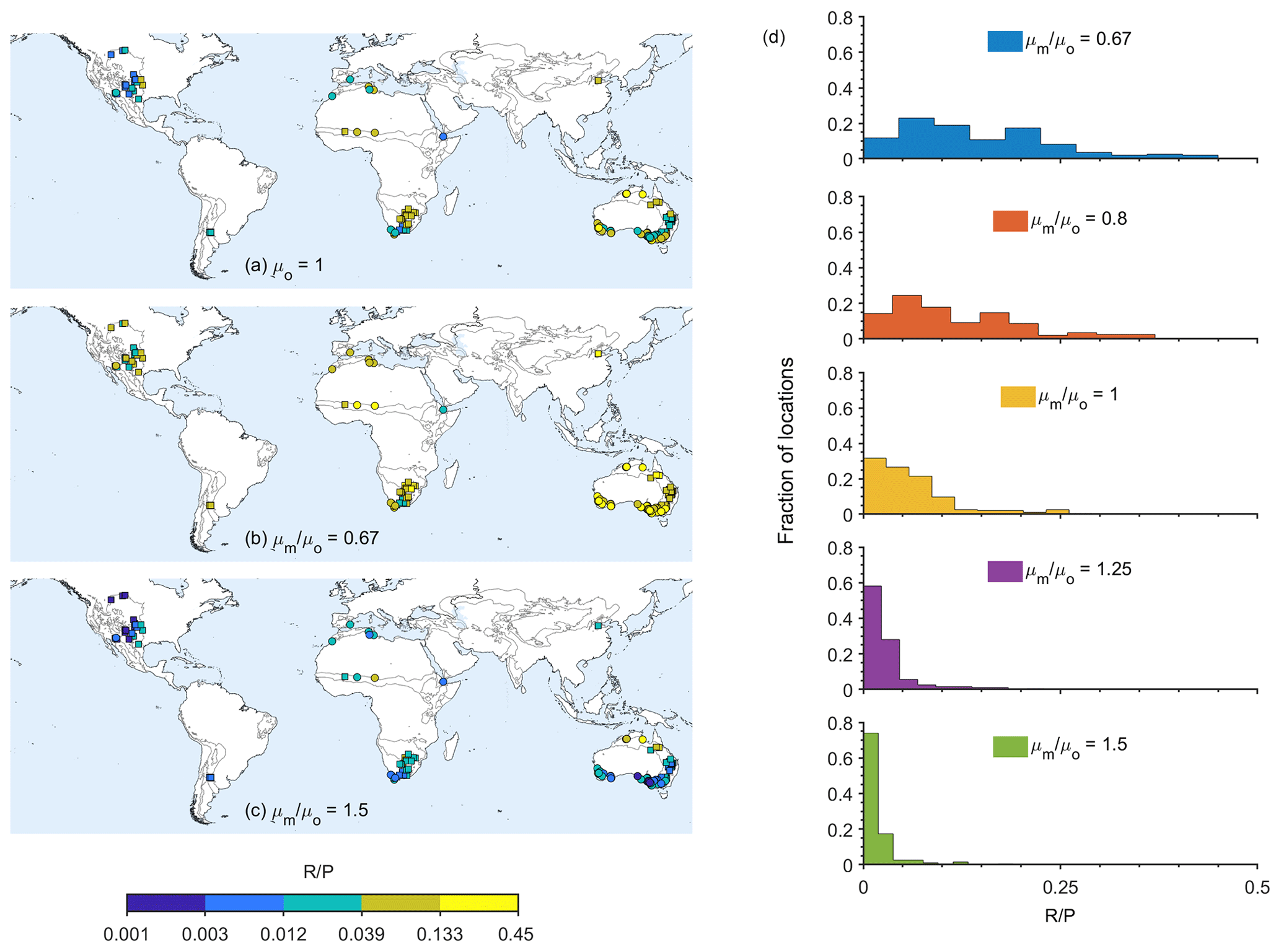
Figure 3 The effect of E_p yearly mean (μ) modification on the $R/P$ ratio. The left panels (a–c) depict the modified ratio in different locations for the mean annual E_p that is measured (a), reduced by a factor of $\mathrm{2}/\mathrm{3}$ (b), and increased by a factor of 1.5 (c). The right panels (d) depict the histograms of the fraction of locations with different $R/P$ ratios under different mean E_p modifications. The ratios between the modified annual mean E_p (μ_m) and the original one (μ₀) are denoted in the figure.

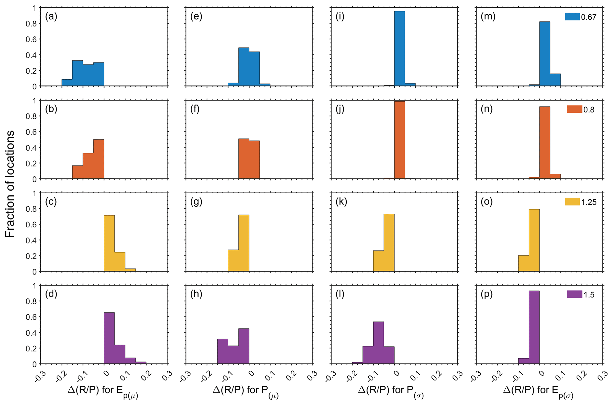
Figure 4 The panels depict the histograms of the change in the ratio $R/P$ ($\mathrm{\Delta }(R/P)=(\frac{R}{P}{)}_{\mathrm{o}}-(\frac{R}{P}{)}_{\mathrm{m}}$; the subscripts o and m correspond to the original and the modified statistics, respectively) for changes in the (a–d) E_p yearly mean, (e–h) P yearly mean, (i–l) P yearly SD, and (m–p) E_p yearly SD. The colors indicate the modification factors, which are the ratios between the modified annual mean (μ_m) or the SD (σ_m) and the original annual mean (μ_o) or SD (σ_o).

Similarly, we considered changes in the mean P (Fig. S3). The annual distribution of the P is not modified, and only the amounts are increased or reduced by the desired multiplicative factor (see the Methods section for details; see also Fig. 2). In Fig. S3, the ratios of $R/P$ in relation to different changes to the mean P are shown. In general, reducing the P results in a higher fraction of locations with a smaller $R/P$ ratio, while increasing the mean P results in a higher fraction of locations with larger ratios. The histograms of the fraction of locations with different changes in the ratio (Fig. 4e–h) reveal a more interesting response. Lowering the mean P results in a mixed response. The $R/P$ ratio decreases in some locations, while it increases in others. In most locations with summer P (92 %, 73 of the considered locations), decreasing the mean annual P results in an increase in the ratio (Fig. 4e and f). The R in these locations is mostly a result of large P events, and the decrease in the mean P hardly affects the fraction of R during these events.

3.2 Effects of changes in the SD

The second change in the statistics of the climate variables that we considered is a change in the SD of the variables while keeping the mean unchanged (see Fig. 2). This is equivalent to uniformly broadening the distribution of the E_p or the P (see the Methods section for details; Fig. 2). We find that increasing the SD of the E_p (Fig. S4) or the P (Fig. S5) results in increasing the $R/P$ ratio in almost all the locations. This is also reflected by the change in the ratio, where most estimated $R/P$ ratios are larger than the original ratios, as indicated by the negative differences (Fig. 4k, l, o, and p).

Reducing the E_p (Fig. S4) or the P (Fig. S5) SD reduces the $R/P$ ratio in most locations. This is illustrated by the positive values of the $R/P$ differences (Fig. 4i, j, m, and n). Overall, the reduction in the SD of the E_p or the P has the smallest effect on the $R/P$ ratio.

3.3 Effects of changes in the frequency of extreme events

Under some future climate predictions, the frequency of extreme events is expected to double (Myhre et al., 2019). Therefore, modifications of the extreme statistics as outlined in Sect. 2.4 were considered. In Fig. 5, the histograms of the fraction of locations with specific $R/P$ ratios are depicted for the doubling of P (panels (a) and (c)) and E_p (panels (b) and (d)) extreme events above the 90 %, 95 %, and 98 % quantiles. For reference, the panels also depict the histogram based on the measured climate conditions. It is apparent in panel (a) that doubling the extreme P events results in more locations with higher $R/P$ ratios. Note that, with this change, the total P is not modified; therefore, the increase in the ratio implies an increase in the actual R. The results are similar in panel (c), where the extreme events of each calendar month were doubled. In Fig. S6, the differences in $R/P$ are presented, showing that, for all the locations considered, increasing the frequency of extreme events increases the R despite the fact that the total P is unchanged. Panel (b) shows that doubling the extreme E_p has a much smaller effect on the R. Preserving the seasonality while doubling the extreme E_p events results in a somewhat stronger effect and more locations with higher R, as shown in panel (d) and Fig. S6. In panels (b) and (d) of Fig. S6, it is shown that, in most locations, doubling the extreme E_p results in larger R, while, in a small fraction of the locations, it reduces the R. Note that these results differ from those of increasing the E_p SD, in which all locations showed an increase in the R.

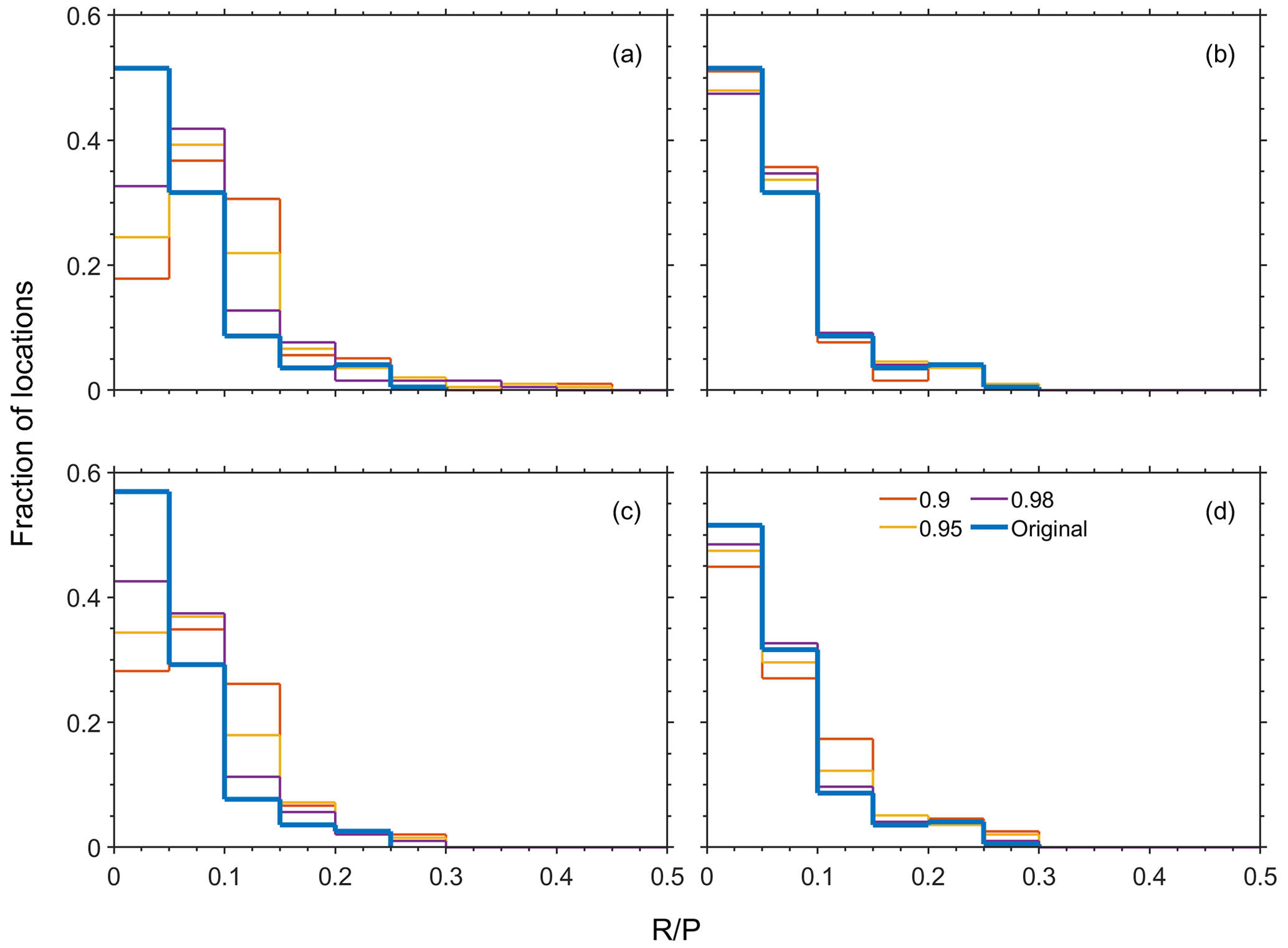
Figure 5 The fraction of locations with the specified $R/P$ ratios due to an increase in the occurrence of annual extreme (a) daily P or (b) daily E_p. The ratios due to an increase in the occurrence of extreme P or E_p events for each calendar month separately are depicted in panels (c) and (d), respectively. See the Methods section for a detailed explanation of the changes to the extreme-event statistics. The values of 0.98, 0.95, or 0.9 represent specified quantiles, where all events above the corresponding values were doubled to establish extreme climate scenarios. The blue line (“original”) corresponds to scenarios with no changes in the extreme statistics.

4 Discussion

Understanding the response of R to varying climate conditions involves a broad range of possible changes to the statistics of the climate variables and renders the task overly complicated. Here, we investigated the effects of various aspects of the climate statistics on groundwater recharge in semi-arid and arid locations. We used the Richards equation (with the VGM hydraulic functions) to simulate the groundwater recharge under varying climate conditions. The use of the Richard equation assumes that groundwater recharge is dominated by diffuse recharge. In regions with significant topography and rocky terrains, considerable runoff is expected (Casenave and Valentin, 1992; Mounirou et al., 2021). Furthermore, in regions where focused recharge and preferential flow paths prevail (van  chaik et al., 2008), using the Richards equation might not accurately capture the dynamics of groundwater recharge (Mirus and Nimmo, 2013; Hartmann et al., 2015, 2017; Appels et al., 2015). Therefore, we limit our analysis to regions where independent estimation of R agreed with our simulated R, suggesting that our method is adequate for these locations. In addition, as expected from the agreement, we found that runoff was not dominant in our simulations.

In our analyses above, we attempted to deal with this complexity by separately considering different changes in climate statistics. Reducing the mean P resulted in mixed outcomes. Some locations illustrated a decrease in the $R/P$ ratio, while, in others, it increased. The increase in the $R/P$ ratio mostly occurred in locations with summer P. Two main explanations are suggested for this counterintuitive change. The first reason is related to the P characteristics in regions with heavy P events that promote deep drainage and R. The decrease in the mean P hardly affects the fraction of R during these events. Therefore, the ratio is increased because the R only decreases slightly, while the P substantially decreases. An additional explanation is associated with reducing the amount of water available for evaporation. The reduction in the amount of P results in longer periods over which the E_a is smaller than the E_p, thereby increasing the fraction of P going to the R (on most days, the E_a is either equal to the E_p when there is a continuum of water reaching the topsoil, and it is close to zero when there is not). Only 25 % of the locations with winter P showed the same behavior – most likely because the E_p during the rainy season is relatively low in these locations, and the effect of the second process mentioned above is weaker. When the mean annual P increases, all locations show a larger $R/P$ ratio (see Figs. 4e–h and S5).

We find that the $R/P$ ratio shows higher sensitivity to changes in the mean E_p than to changes in the mean annual P. The P is equal to the sum of the R and E_a under the assumption that, in a steady state, the change in the total soil water storage is negligible and the assumption that the runoff is negligible (this was verified for the locations considered in this study). Mathematically, we express it as follows:

$$\begin{array}{}\text{(6)}& R=P-E_{\mathrm{a}},\end{array}$$

and, therefore,

$$\begin{array}{}\text{(7)}& {\displaystyle \frac{R}{P}}=\mathrm{1}-{\displaystyle \frac{E_{\mathrm{a}}}{P}}.\end{array}$$

If one assumes that the evapotranspiration is a function of the ratio $E_{\mathrm{p}}/P$ (Budyko, 1974), the changes in $R/P$ are expected to be the same regardless of whether the change in E_a is due to changes in E_p or changes in P. However, if E_a depends not only on $E_{\mathrm{p}}/P$ but also on the actual water content of the top soil layer (Gerrits et al., 2009), one can expect different sensitivity to changes in E_p or changes in P, as we observed.

The response to changes in the P SD is easily understood considering the fact that most of the R is triggered by large P events. The increase in the $R/P$ ratio due to an increase in the E_p SD can be attributed to the fact that, in some years, the E_p becomes small enough to allow significant R, while during the years with higher E_p, the reduction in R is much smaller because there is not always water available for E_a; i.e., larger values of E_p do not affect the E_a because it has already reached an upper limit. Ultimately, we found that changes in the statistics of extreme rainfall events have a much greater effect on R than in extreme E_p events.

5 Conclusions

Understanding the combined effects of all the changes in climate variables on groundwater recharge is an ongoing effort and is expected to play a critical role in future studies. Many factors affect groundwater recharge, making it a complicated process to quantify. Some of these processes are hard to predict, and others are related to human activity affecting, directly (such as urbanization) and indirectly (such as deforestation), the fraction of precipitation infiltrating deep soil levels. Anthropogenic factors, such as land use changes, are expected to strongly affect groundwater recharge. Those changes are expected to occur much faster than changes in climate statistics. In our study, we examined the effects of changes in climate statistics, i.e., non-anthropogenic, on groundwater recharge in arid and semi-arid regions.

We considered locations worldwide. The selected locations are characterized by bare soil or sparse vegetation to avoid the effect of water loss due to transpiration. Furthermore, the site selection process included comparisons of simulated and reported yearly groundwater recharge fluxes to verify that only sites for which the model represents the natural conditions are considered and that locations influenced by factors such as human disturbances are excluded. Despite the simplicity of the modeling approach, we found that, in many places, worldwide, the model provides good estimates of the fraction of precipitation infiltrating deep soil.

Our simulations show that changes in climate statistics may have various effects on groundwater recharge. In most locations, increasing the mean P results in higher $R/P$ ratios and vice versa, while increasing the mean E_p reduces the $R/P$ ratio and vice versa. Increasing the SD of both P and E_p results in a higher $R/P$ ratio. In most locations, doubling the frequency of extreme P or E_p events results in a higher $R/P$ ratio. However, the effect of more frequent P events is stronger than the effect of more frequent E_p events.

Previous studies suggested different trends and changes in future groundwater recharge. The differences between the projected climate statistics used in those studies may explain those seemingly contradictory assessments of future groundwater recharge fluxes. To enhance our understanding and better explain the predicted groundwater recharge changes, results should be augmented by an analysis of the projected changes in potential evapotranspiration and rainfall statistics. As demonstrated above, considering only changes in the mean and the SD is not enough, and changes in the statistics of extreme events are essential. This is attributed to the non-linear responses of groundwater recharge to changes in climate statistics. The conclusions drawn in this analysis are valid for locations where diffuse recharge dominates the overall recharge. In areas where groundwater recharge occurs predominantly through focused processes (e.g., preferential flow and recharge of runoff at specific locations on the landscape), future analyses should include additional factors at the sub-catchment scale, such as topographic attributes and spatiotemporal variability in precipitation. Separate studies are required to investigate the effects of climate change on groundwater recharge in humid regions or in agricultural fields, where the root uptake and the transpiration are significant.