Developing water supply reservoir operating rules for large-scale hydrological modelling

Reservoirs are ubiquitous water infrastructure, providing functional capability to manage, and often mitigate, hydrological variability across space and time. The presence and operation of a reservoir control the downstream flow regime, such that in many locations understanding reservoir operations is crucial to understanding the hydrological functioning of a catchment. Despite many advances in modelling reservoir operations, inclusion of reservoirs in large-scale hydrological modelling remains challenging, particularly when the number of reservoirs is large and data access is limited. Here we design a set of simple reservoir operating rules (with only two calibrated parameters) focused on simulating small water supply reservoirs across large scales with various types of open-access data (i.e. catchment attributes and flows at downstream gauges). We integrate our rules into a national-scale hydrological model of Great Britain and compare hydrological simulations with and without the new reservoir component. Our simple reservoir operating rules significantly increase model performance in reservoir-impacted catchments, particularly when the rules are calibrated individually at each downstream gauge. We also test the feasibility of using transfer functions (which transform reservoir and catchment attributes into operating rule parameters) to identify a nationally consistent calibration. This works well in ∼ 50 % of the catchments, while nuances in individual reservoir operations limit performance in others. We suggest that our approach should provide a lower benchmark for simulations in catchments containing water supply reservoirs and that more complex methods should only be considered where they outperform our simple approach.

1 Introduction

Effective and reliable water resource management is essential for food, water and energy security (Sardo et al., 2023; Carrillo and Frei, 2009; Brown et al., 2015). To cope with increasing hydrologic variability and to ensure a reliable supply of water, national- to continental-scale solutions are needed (McMillan et al., 2016). This requires more integrated and resilient water resource systems which can manage, and often mitigate, hydrological variability across space and time (Dobson et al., 2020; Wendt et al., 2021; Gaupp et al., 2015). A key part of these interconnected water management systems is reservoirs. Reservoirs play a vital role in the supply and management of water resources, and their operations significantly alter downstream flow (Döll et al., 2009; Tebakari et al., 2012; Vörösmarty et al., 2003; Adam et al., 2007; Salwey et al., 2023). As a result, appropriately representing reservoirs and their operating rules in hydrological modelling frameworks is a key area of research (Brown et al., 2015).

To model reservoir operations at the largest scale, global reservoir databases and uncalibrated operating rules are available (Hanasaki et al., 2006; Wisser et al., 2010; Lehner et al., 2011b). By simulating how much water is released from a reservoir at each time step, uncalibrated reservoir operating rules integrated into global hydrological models have been shown to yield significant improvements in streamflow simulations (Abeshu et al., 2023; Hanasaki et al., 2006). However, global reservoir rules and datasets are often not suitable for application over national/continental scales. Using Great Britain (GB) as an example, the distribution of both reservoir type and size is markedly different when comparing data from global (Global Reservoir and Dam Database, GRanD) and national (UK Reservoir Inventory) reservoir databases (Fig. 1). Over three-quarters of the reservoirs in GB are designed for water supply, whereas globally reservoirs are primarily designed for irrigation (33 %) and/or hydropower (31 %). Furthermore, reservoirs in global databases (GRanD) tend to be much larger than in the UK Reservoir Inventory. Consequently, reservoir operating rules developed from these global databases, for global-scale application, are often unsuitable for applications in national-scale models.

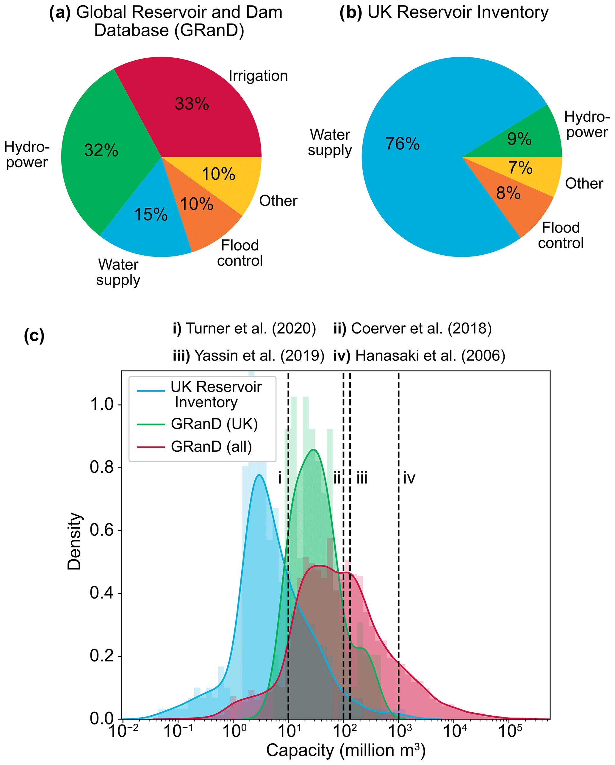
Figure 1 (a, b) Pie charts showing the distribution of reservoir types across the (a) GRanD database and (b) UK Reservoir Inventory. The “Other” category groups together reservoirs designed for uses such as recreation, navigation and fishing which make up a small proportion of the database. (c) Histogram showing the distributions of reservoir capacities across the UK Reservoir Inventory (blue), UK reservoirs in GRanD (green) and the full GRanD database (red). Dashed lines and associated labels (i–iv) represent the smallest reservoirs considered by some key papers discussed in the Introduction.

One option for developing more tailored reservoir operating rules at the national scale is to use a calibrated, data-driven approach. ResOpsUS (Steyaert et al., 2022) is a national US dataset providing historical time series of reservoir storage, outflow and inflow for over 600 US reservoirs. This dataset has enabled the development of a national-scale inventory of tailored, empirically derived, operating rules for each reservoir (Turner et al., 2021). When forced with observed inflow data, these data-driven rules reproduce downstream flow observations significantly better than uncalibrated, generic operating rules (Turner et al., 2020). However, these data-driven operating rules no longer outperform the generic alternatives when integrated into a hydrological model, i.e. when forced with simulated inflows (“online testing”) instead of observed ones (“offline testing”) (Turner et al., 2021). Furthermore, extensive datasets such as ResOpsUS are seldom available at the national scale; consequently, the approach is challenging to apply elsewhere.

In this paper, we develop a set of simple reservoir operating rules tailored towards water supply reservoirs that can be implemented across local, national or global scales. We focus on water supply reservoirs as there is a lack of generic operating rules for this type of reservoir, despite their importance for water supply and management in many countries, including our application domain (Great Britain). Although offline testing of operating rules is common in the literature (Zhao et al., 2016; Yassin et al., 2019), here we integrate and test reservoir representation in a hydrological model from the start.

Our simple operating rules have parameters which are linked to catchment and reservoir attributes via transfer functions. Parameter regionalization, where transfer function parameters are calibrated by assuming prior relationships between model parameters and catchment attributes, is common in hydrological modelling (Samaniego et al., 2010) but has not previously been applied to modelling reservoir operating rules. We present the results from two methods of calibration. The first method uses common bounds for the transfer function parameters but within these bounds finds an “optimal” parameter set for each catchment (we call this a catchment-by-catchment calibration). The second method identifies one set of the optimal transfer function parameters that can be estimated and applied across all reservoirs (we call this a nationally consistent calibration). This latter method facilitates the simulation of operating rules in ungauged or data-poor basins. The simplicity of our rules and use of transfer functions allow us to simulate reservoir operations over hundreds of reservoirs using only open-access data.

2 Developing large-scale reservoir operating rules

The following section describes the generic reservoir operating rules introduced in this paper for the large-scale simulation of water supply reservoirs. We discuss their specific application to Great Britain in Sect. 3.

Operating rules

As is common in modelling reservoirs, we consider reservoirs to be zero-dimensional points, where their dynamics are controlled by a mass balance equation. The reservoir mass balance is updated at every time step and represented with the following equation:

$$\begin{array}{}\text{(1)}& {\displaystyle \frac{\mathrm{\Delta }S}{\mathrm{\Delta }t}}=I_t-{\mathrm{CF}}_t-{\mathrm{ABS}}_t-{\mathrm{spill}}_t,\end{array}$$

where S represents the reservoir storage and t is time. I_t is the inflow simulated by the hydrological model per unit time, CF_t is the volume per unit time of water released into the downstream river to fulfil environmental flow requirements (known as the compensation flow), ABS_t is the volume per unit time of water abstracted from the reservoir for public water supply and spill_t is the volume of water remaining above the reservoir capacity per unit time which must be released downstream (this is calculated after all other fluxes have been calculated). Equation (1) does not include evaporation as this is not a big component of the mass balance for reservoirs in Great Britain (see Sect. 3.4) (Dobson et al., 2020); however, evaporation could easily be included in the mass balance for reservoirs where this is important.

We use transfer functions to determine the relationships between catchment attributes (e.g. catchment size or mean annual rainfall), reservoir attributes (e.g. capacity or use), and the rates of compensation flow (CF) and abstraction (ABS) as follows:

$$\begin{array}{}\text{(2)}& {\displaystyle }\begin{array}{rl}\mathrm{ABS}=& f_{\mathrm{1}}(\mathrm{catchment}\mathrm{attributes},\mathrm{reservoir}\mathrm{attributes},\\ & {\mathrm{parameter}}_{\mathrm{1}\mathrm{\dots }n}),\end{array}\text{(3)}& {\displaystyle }\mathrm{CF}=f_{\mathrm{2}}(\mathrm{catchment}\mathrm{attributes},{\mathrm{parameter}}_{\mathrm{1}\mathrm{\dots }n}).\end{array}$$

The catchment and reservoir attributes used within these functions will vary depending on what data are available, and a selection of attributes may have to be tested before a sensible relationship is established. In some cases attributes may be combined (e.g. by normalizing reservoir storage by catchment area). In this study, we calibrate the parameters in the transfer functions above both in a catchment-by-catchment manner and nationally, identifying one parameterization for the entire sample of catchments. The development of the transfer functions for our study area (Great Britain) is described in more detail in Sect. 3.5.1. The compensation flow and abstraction fluxes at each time step, CF_t and ABS_t, are then calculated (in m³ d⁻¹) based on the current reservoir storage as follows:

$$\begin{array}{}\text{(4)}& {\displaystyle }{\mathrm{CF}}_t=\left\{\begin{array}{ll}\mathrm{CF}& \mathrm{if}{S}_t>S_{\min }+CF\cdot \mathrm{\Delta }t,\\ (S_t-S_{\min })/\mathrm{\Delta }t& \mathrm{if}{S}_{\min }<S_t<S_{\min }+\mathrm{CF}\cdot \mathrm{\Delta }t,\\ \mathrm{0}& \mathrm{if}{S}_t\le S_{\min },\end{array}\right\}\text{(5)}& {\displaystyle }{\mathrm{ABS}}_t=\left\{\begin{array}{ll}\mathrm{ABS}& \mathrm{if}{S}_t>S_{\min }+\mathrm{CF}\cdot \mathrm{\Delta }t+\mathrm{ABS}\cdot \mathrm{\Delta }t,\\ (S_t-S_{\min })/\mathrm{\Delta }t-\mathrm{CF}& \mathrm{if}{S}_{\min }<S_t<S_{\min }+\mathrm{CF}\cdot \mathrm{\Delta }t+\mathrm{ABS}\cdot \mathrm{\Delta }t,\\ \mathrm{0}& \mathrm{if}{S}_t\le S_{\min }+\mathrm{CF}\cdot \mathrm{\Delta }t.\end{array}\right\}\end{array}$$

In this instance, CF_t is given priority and removed before ABS_t; hence, the calculation of ABS_t must ensure there is enough storage for the CF_t to be removed first. This step ensures there is sufficient storage for these fluxes to be removed and prevents the reservoir from being drained below its minimum capacity S_min (which can be either specified using site-specific data or estimated as a percentage of total reservoir capacity). Note that whilst in this study we use fixed values for CF and ABS over time, seasonal or sub-seasonal transfer functions could be developed to vary these parameters over time if appropriate.

To implement these operating rules into a hydrological model, the user will need data describing reservoir use (in this case the reservoir ought to be designed for water supply), capacity (to represent storage) and location (to locate the reservoir on the river network). These data can be obtained nationally, from datasets such as the UK Reservoir Inventory (Durant and Counsell, 2018), Inventory of dams in Germany (Speckhann et al., 2021) or National Inventory of Dams in the USA (U.S. Army Corps of Engineers, 2023), or globally, from datasets such as GRanD (Lehner et al., 2011b) and GeoDAR (Wang et al., 2022). In order to define the transfer functions used in the operating rules above, a small sample of observed compensation flow and abstraction data are needed (ideally for at least 10 reservoirs). These data can be found in documents published by water companies (e.g. water resource management plans (WRMPs) or drought plans) and academic literature, or (where a gauge is located close to a reservoir outflow) they can be inferred from the downstream flow time series.

3 Application to national-scale hydrological modelling in Great Britain

The following section describes the application of the simple operating rules introduced above to the national-scale hydrological modelling of Great Britain (GB). Like many other countries, GB faces increasing water scarcity, where changing patterns of rainfall and evapotranspiration could add to the increasing pressures of future demand (Watts et al., 2015; Dobson et al., 2020). At present, water management is carried out mostly by local water companies, but to ensure water supply remains resilient to change, GB is considering several more regional or national strategic solutions (Murgatroyd and Hall, 2020). Reservoirs make up a large component of the domestic water supply system in GB and have a significant influence on river flows (16 % of all river basins contain one or more reservoirs) (Salwey et al., 2023; Tijdeman et al., 2018). Due to the size and type of reservoirs found across GB (mostly small water supply reservoirs), global-scale approaches to reservoir representation are not applicable. This serves as a good case study for somewhere where existing reservoir operating rules are not suitable and where the national context of water management is particularly important.

To demonstrate the application of our reservoir operating rules across GB, the rules are implemented in the DECIPHeR hydrological model (Sect. 3.1). We use hydrometeorological data from 1970–2020 (Sect. 3.2) to run model simulations in two samples of catchments: reservoir catchments, i.e. all those catchments draining into a gauge that lies downstream of one or more water supply reservoirs, and near-natural catchments, which have no upstream reservoirs (Fig. 2). The near-natural simulations use multiscale parameter regionalization (MPR) (Mizukami et al., 2017; Samaniego et al., 2017; Lane et al., 2021) to estimate DECIPHeR's natural model parameters. When using the term “natural model parameters”, we refer to the seven standard DECIPHeR parameters which are designed to simulate hillslope hydrology un-impacted by humans (Sect. 3.3). In the reservoir catchments, DECIPHeR is run both with and without reservoir representation (Sect. 3.4 and 3.5) to compare the difference in model performance before and after incorporating our new reservoir operating rules (Sect. 3.6). Since most national-scale models of GB do not include reservoir representation (e.g. G2G or GR4J (Smith et al., 2019; Rudd et al., 2019)), we consider this to be a suitable benchmark. Finally, the model is evaluated against a suite of model performance metrics (Sect. 3.6) to better understand where and when our simple reservoir operating rules result in better (or worse) model performance and to act as a benchmark for future model improvements.

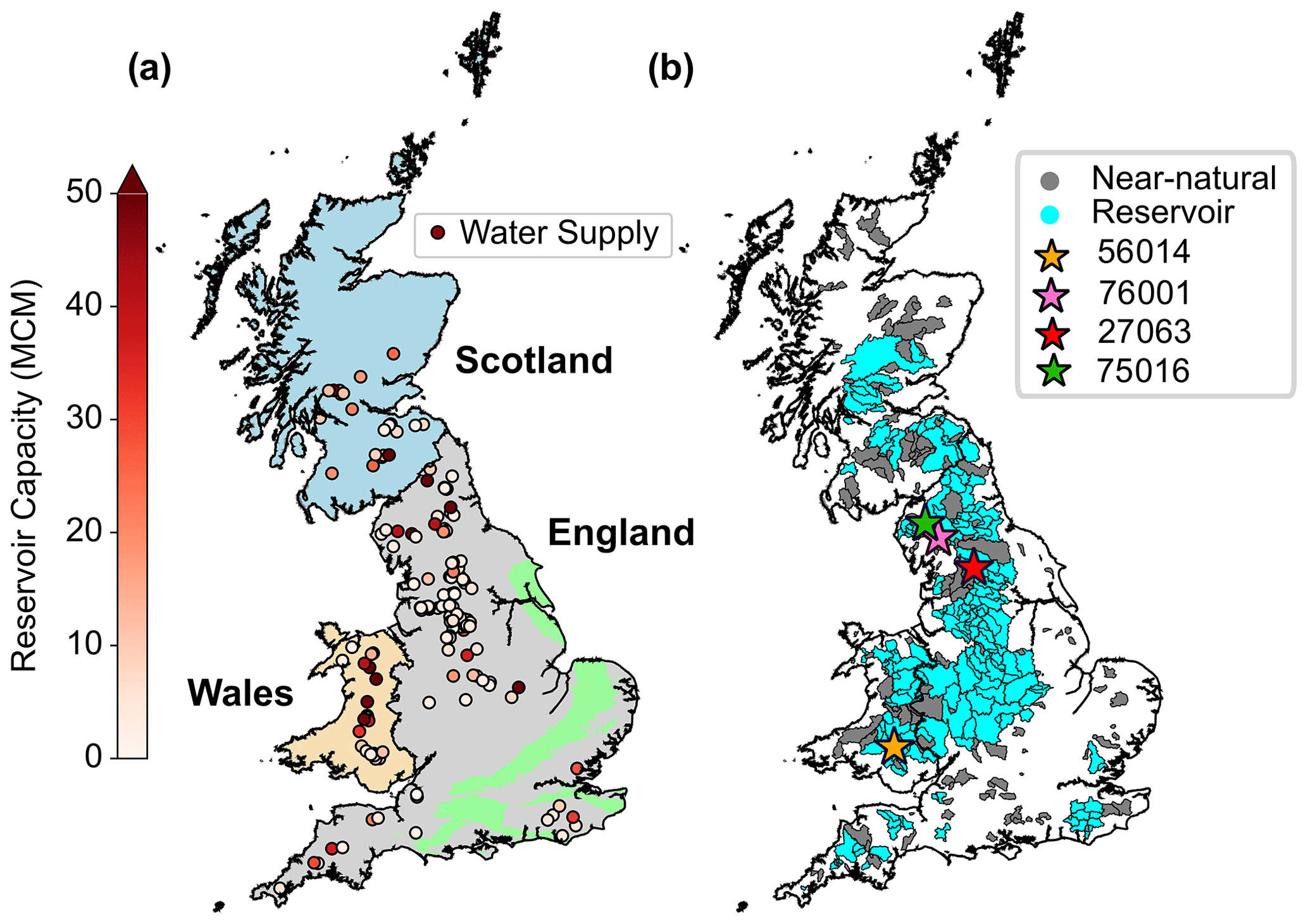
Figure 2 Distribution of (a) water supply reservoirs across GB and (b) near-natural and reservoir catchments used in this study. Reservoirs are coloured by their storage capacity, and the four catchments featured in Figs. 5–8 are highlighted with stars in panel (b).

3.1 DECIPHeR

DECIPHeR (Dynamic fluxEs and ConnectIvity for Predictions of HydRology) is a flexible, semi-distributed hydrological modelling framework which has previously been implemented across a range of scales (e.g. catchment to national scales) and locations (e.g. Europe, Asia, Africa) and has both been coupled to other models and had additional modules incorporated (Shannon et al., 2023; Dobson et al., 2020; Devitt, 2019; Fadhliani et al., 2021). The model has been applied nationally in Great Britain and demonstrated good performance (Lane et al., 2021; Coxon et al., 2019a), with generally better model performance in wetter catchments in the north and west of GB. However, since the model has no reservoir representation, performance is usually poor in catchments downstream of reservoirs. At present, in these locations the model has no knowledge of reservoir locations, and flow in these catchments is simulated as if reservoirs were natural.

DECIPHeR uses hydrological response units (HRUs) to split the landscape into non-contiguous spatial elements that share similar characteristics in landscape attributes (e.g. soil, topography or geology) and spatially varying inputs (e.g. rainfall). Each HRU then acts as a separate model store capable of having different spatial inputs, model parameter values, and/or model structures to represent different and localized processes. In this study, HRUs were classified using a 2.2 km input grid (consistent with national climate projection data) and were further subdivided by gauged sub-catchments (which include those defined by reservoir nodes) and percentiles of slope and upslope accumulated area (i.e. the area of land draining to a particular point in the landscape). This ensures that HRUs cascade downslope to the bottom of the valley and that the spatial variability of the climatic inputs is appropriately represented.

3.2 Hydrometeorological data

To drive the hydrological model, precipitation and potential evapotranspiration (PET) time series are needed. In this study, we use observation-based gridded daily precipitation and PET data derived from the HadUK-Grid dataset, which provides a number of climate variables on a 1 km × 1 km grid across the UK (Hollis et al., 2019). Daily precipitation data from HadUK-Grid are available from 1891 to the present and derived from the Met Office UK rain gauge network. The observed precipitation data from the rain gauge network are quality-controlled, and then inverse-distance-weighted interpolation is used to generate the daily rainfall grids (Hollis et al., 2019). Daily PET was calculated using the Penman–Monteith equation applied to climate variables available from HadUK-Grid (Robinson et al., 2023). These data are available from 1969–2021. While the climatic variables are available on a 1 km × 1 km grid, these were upscaled to a 2.2 km grid for use in the hydrological modelling. This was chosen to align with the existing model setup and the grid used for national climate projections (Robinson et al., 2021; Lane and Kay, 2022).

In this study, we run the model from 1970–2020 since it encompasses a variety of climatic conditions. The first 5 years of the time window was used as a spin-up period where no model evaluation is carried out. Simulations are evaluated from 1975 onwards (or from the date the reservoir construction was completed) using daily streamflow time series from the UK National River Flow Archive (NRFA) (https://nrfa.ceh.ac.uk/, last access: 9 September 2024). Since 96 % of reservoirs in GB were built by 1980, we can evaluate the model performance across most of the simulated period (where the flow data are available at the relevant gauge).

3.3 Calibration in near-natural catchments

In this study, we calibrate the parameters in the reservoir operating rules independently from the natural model parameters. This avoids unrealistic parameterizations or equifinality, where natural parameters might mimic reservoir processes (Dang et al., 2020).

DECIPHeR has seven natural model parameters which describe how much water the soils can store and how permeable they are, the river channel velocity, and the transmissivity of the sub-surface (Coxon et al., 2019a). To generate nationally consistent parameter fields for DECIPHeR's natural model parameters, we use multiscale parameter regionalization (MPR), following the method introduced by Samaniego et al. (2010) and applied in DECIPHeR by Lane et al. (2021). High-resolution parameter fields are generated by linking model parameters to spatial catchment characteristics via transfer functions and subsequently using MPR to upscale the parameter fields to the model resolution. Transfer functions were defined for each natural model parameter (see Lane et al., 2021), and the transfer function parameters were calibrated simultaneously across all non-reservoir (or near-natural) catchments. Catchments with reservoirs were excluded from this calibration, as the purpose was to find parameter fields which resulted in good model performance for natural catchments before the addition of any reservoir component.

We calibrated the transfer function parameters using a set of simulations in near-natural catchments selected from the UK benchmark network (Fig. 2b). The UK benchmark network (Harrigan et al., 2018) consists of 137 catchments chosen for their lack of human influence and near-natural flow regime. In each catchment, we ran 5000 simulations sampling the transfer function parameters between set bounds. The top 10 natural transfer function parameter combinations were then chosen by calculating the non-parametric Kling–Gupta efficiency (KGE) (Pool et al., 2018) (see Sect. 3.6) in all near-natural catchments. The 10 combinations with the highest average non-parametric KGE across all the near-natural catchments were subsequently used to determine the natural model parameters in reservoir catchments.

3.4 Integrating reservoirs into the river network

To integrate new reservoir representation into DECIPHeR, we modified the river routing and represent each reservoir as a zero-dimensional point on the river network. Channel flow routing in DECIPHeR is modelled using a set of time delay histograms for the points on the river network where river flow time series are required. A fixed channel wave velocity is applied throughout the network to account for delay and attenuation in the simulated flows. The reservoir points are placed at their outflow locations as nodes on the river network. These nodes break up the river reach such that, during a simulation, incoming river flow is manipulated according to the operating rules described in Sect. 2.1 before it continues downstream. Reservoir storage is also simulated, and the time series can be obtained as an output. In this study, we do not consider evaporation from the reservoirs; this is partly because the flux is small in GB and partly because we model reservoirs as zero-dimensional points, and so we already simulate evaporation from the underlying area. We do not have evaporation relationships or surface area data, and we note that other studies also opted to exclude evaporation from reservoirs across Great Britain, where even the largest reservoir (Kielder Water) only has evaporation equal to 3 % of its inflow (Dobson et al., 2020).

We use a 50 m gridded digital elevation model (Intermap Technologies, 2009) to generate the river network in DECIPHeR, extracting headwater cells from an open-access river network which maps the rivers across GB, generated by the Ordinance Survey (Ordnance Survey, 2023). These cells are then routed downstream to generate a river network. Once the river network has been generated, reservoir locations and capacities were extracted for water supply reservoirs from the UK Reservoir Inventory (Durant and Counsell, 2018), which contains data on UK reservoirs with storage exceeding 1.6×10⁶ m³ (or MCM for million cubic metres) and a selection of smaller ones. After cross-referencing the UK Reservoir Inventory with the Global Reservoir and Dam Database (Lehner et al., 2011a), we found that some of the Scottish reservoirs in GRanD were not included in the UK Reservoir Inventory, and in several locations the capacities were significantly different. Consequently, in Scotland, the UK Reservoir Inventory has been supplemented with data from the Scottish Environment Protection Agency (SEPA). This provided an additional four water supply reservoirs, and where mismatches in capacities were identified, the UK Reservoir Inventory has been updated using the supplementary SEPA data.

In total, 207 reservoirs from the UK Reservoir Inventory were classified as water supply. We excluded 47 of the UK Reservoir Inventory water supply reservoirs from this analysis, either because there was no gauge downstream of the reservoir and thus results could not be evaluated (11); because they were outside of Great Britain (2); or because they could not be placed on the river network (34), which was usually because the reservoir appeared to be disconnected from the river channel.

3.5 Simulations in reservoir catchments

Simulations in reservoir catchments are carried out for all gauges located downstream of one or more water supply reservoirs. This is a total of 264 catchments (Fig. 2b). In each catchment, the model is run both with and without reservoir representation. The no-reservoir scenario runs 10 simulations in each reservoir catchment using the top 10 natural transfer function parameter combinations (Sect. 3.3). In the reservoir scenario, for each of the same 10 parameter combinations, we sample the reservoir parameters 500 times, resulting in 5000 simulations per catchment. The minimum capacity of each reservoir (S_min) is set to 10 % of the maximum capacity (which is obtained from relevant databases). At the very start of a simulation, S_t is set to 90 % of the reservoir's maximum capacity (since simulations begin in winter when reservoirs are usually full).

3.5.1 Defining reservoir transfer functions

In order to define the reservoir transfer functions, we used a small sample of catchments for which compensation flow data and abstraction estimates are available to determine which catchment and reservoir attributes (e.g. catchment area, rainfall, reservoir capacity) exhibit the strongest relationships with the fluxes (see Sect. 4.2 for the chosen attributes). The small sample consists of 9 catchments with compensation flow data and 16 with abstraction estimates. Although data for these fluxes are not available on a large scale, in some cases compensation flow is recorded in water resource management plans and drought plans; where there is a suitable downstream gauge, hydrological signatures can be used to infer abstraction volume (by looking at changes to the water balance) and compensation flow (from plateaus in the flow duration curve) (see Sect. S1 in the Supplement). In this study, abstraction and compensation flow remain constant throughout the simulation (i.e. the same volume is released or abstracted at every time step), but where appropriate they could be varied throughout the year.

Since they are based on only a limited number of observed data points, the transfer functions and the data they use contain significant uncertainty. To account for this, we define upper and lower bounds for each transfer function parameter (p) and sample within the chosen parameter space. The upper and lower bounds are determined after assessing the relationship between the non-parametric KGE and the two parameters (ABS and CF) in a selection of catchments (see Sect. S2). By using transfer functions which account for local information, we avoid sampling unrealistic parameter space and can begin to understand how these fluxes might be estimated without calibration.

3.5.2 Calibration of reservoir parameters (catchment-by-catchment and nationally consistent calibration)

After running 5000 simulations in each catchment, we consider two types of calibration. The first is a catchment-by-catchment calibration for which we identify the best-performing simulation and set of reservoir parameters in each catchment (this could leave us with a different optimal reservoir transfer function parameter combination in each catchment). The second looks for the best nationally consistent calibration, where each catchment uses the same set of reservoir transfer function parameters. The best nationally consistent simulation is chosen by first calculating the difference in non-parametric KGE between each of the 5000 reservoir simulations and the best no-reservoir simulation and then identifying the median difference in KGE for each of the 5000 simulations across all of the catchments with a contributing area of more than 25 % (i.e. more than 25 % of the catchment is drained through a reservoir). We chose to only use gauges draining a high proportion of the catchment since these are the most impacted by the reservoir representation, but note that the results are very similar if we include more or fewer gauges in this sample (see Sect. S5). The simulation with the highest median KGE difference was then chosen as the best nationally consistent calibration.

3.6 Model evaluation

To evaluate the flow simulations in the both the benchmark and reservoir catchments, we use the non-parametric KGE (Pool et al., 2018; Gupta et al., 2009). The non-parametric KGE metric is comprised of three diagnostically meaningful components considering the errors in mean flow, flow variability, and the correlation between observed and simulated flow. The non-parametric KGE uses the flow duration curve to investigate flow variability instead of the standard deviation and the Spearman rank correlation instead of the Pearson correlation coefficient. Since previous work (Ferrazzi and Botter, 2019; Salwey et al., 2023) has shown that reservoirs can have a significant impact on the flow duration curve and water balance, we considered this to be a suitable metric to investigate the flow components in both benchmark and reservoir catchments. We also calculated the normalized mean absolute error (nMAE) to complement the Spearman rank correlation, which was more informative in catchments with little variability in river flows (see Sect. 4.3).

Flow time series are only evaluated at gauges where there is more than 20 years of observed data between 1975 (or the reservoir construction date if this is later) and 2020. After these criteria have been enforced, we are able to evaluate the model in 205 out of 264 catchments. The model is evaluated for both the catchment-by-catchment calibration and the nationally consistent calibration by comparing simulations with and without reservoir representation.

For completeness, in a few selected catchments we also compared our operating rules to the widely used non-irrigation reservoir rule introduced by Hanasaki et al. (2006). However, since the Hanasaki rule assumes that no abstractions are taken directly from the reservoir, this rule is not well suited to water supply reservoirs in our domain (see Sects. 4.3 and S8). We could not compare our operating rules to any of the data-driven approaches in the literature (e.g. Turner et al., 2020), since their high data requirements could not be fulfilled at the national scale in GB. Comparing the simulations which use our new operating rules to the simulations of the pre-existing hydrological model without reservoir representation thus remains the most feasible and relevant way to evaluate the new proposed model.

4 Results

4.1 Calibration in near-natural catchments

Model performances from simulations in near-natural catchments with the top (highest median non-parametric KGE across 137 catchments) nationally consistent calibration are displayed in Fig. 3. When considering the top 10 near-natural simulations across all 137 catchments, the median KGE score ranges from 0.83–0.84. While the model generally captures the mean flow, flow variability and correlation well, there are some catchments which have poor performance. For example, the Aldbourne at Ramsbury (39101) and the Ewelme at Ewelme Brook (39065) (which are both chalk catchments) have non-parametric KGE scores of −0.69 and −0.11 in the best-performing simulation, respectively. In general, the poorer-performing catchments are largely chalk catchments, since here the model is not able to capture flow losses from inter-catchment groundwater flows, which has also been noted in previous studies (Coxon et al., 2019a; Lane et al., 2021, 2019). While this is an area of model improvement for future studies (see, for example, Oldham et al., 2023), it is less significant for this study as reservoirs are typically not constructed in groundwater-dominated catchments in GB.

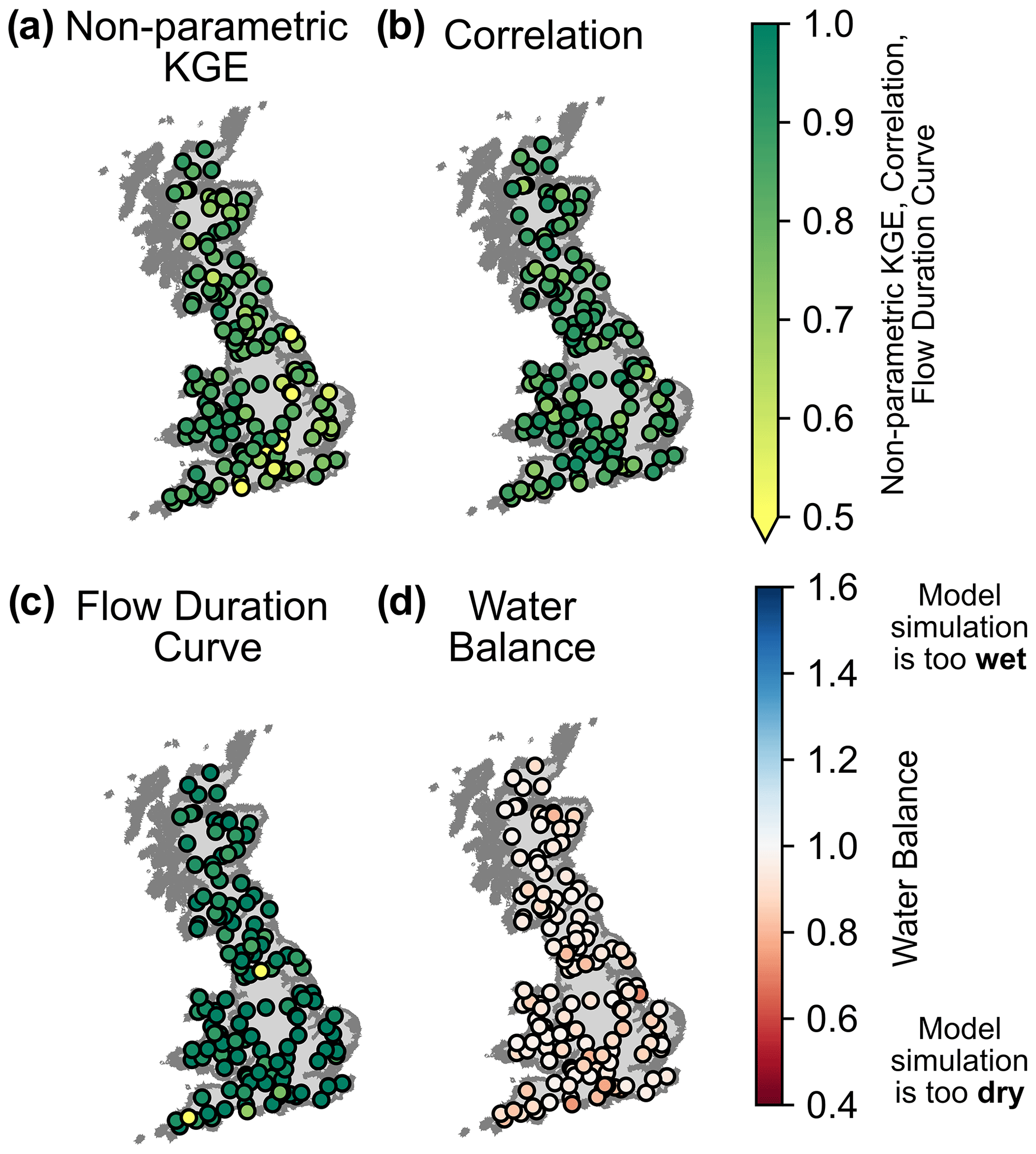
Figure 3 (a) Non-parametric KGE and its components (b, c, d) for the transfer function parameter combination with the highest median KGE (0.84) across 137 near-natural catchments.

4.2 Reservoir transfer function definition

We tested a number of catchment/reservoir attributes to define the reservoir transfer functions used in this study (see Sect. S1), relying on data from a small sample of catchments (see Sect. 3.5.1). We found that catchment area was the most appropriate attribute to identify the compensation flow (CF), and the upstream reservoir capacity was best for identifying the abstraction volume (ABS) (see Fig. 4 and Eqs. 6 and 7 below). Since the observations (Fig. 4) do not show any evidence of non-linearity, we chose to use a linear (and hence more parsimonious) relationship for both transfer functions:

$$\begin{array}{}\text{(6)}& {\displaystyle }\mathrm{ABS}=\mathrm{ResCapacity}\cdot p_{\mathrm{1}},\text{(7)}& {\displaystyle }\mathrm{CF}=\mathrm{CatchArea}\cdot p_{\mathrm{2}}.\end{array}$$

The top nationally consistent calibration associated with the ABS parameter (marked in Fig. 4a with a dashed grey line) generates parameters which are similar to those observed in the literature. However, the top nationally consistent transfer function selected for estimating the CF parameter (marked in Fig. 4b with a dashed grey line) lies close to the upper end of the sampling limits (Table 1) and does not match the observations. To investigate the sensitivity of the model to each of the reservoir parameters (CF and ABS), Fig. 4 also shows the variability in the transfer functions associated with the top 5 % of nationally consistent simulations (this is displayed in Fig. 4 with darker shading). The top 5 % of simulations are those with the highest average non-parametric KGE (calculated across the full sample of reservoir catchments). This shows that the model's predictive performance is more sensitive to ABS (p₁) than CF (p₂). The regional differences in the transfer function parameters selected by the catchment-by-catchment calibration can be seen in Sect. S9.

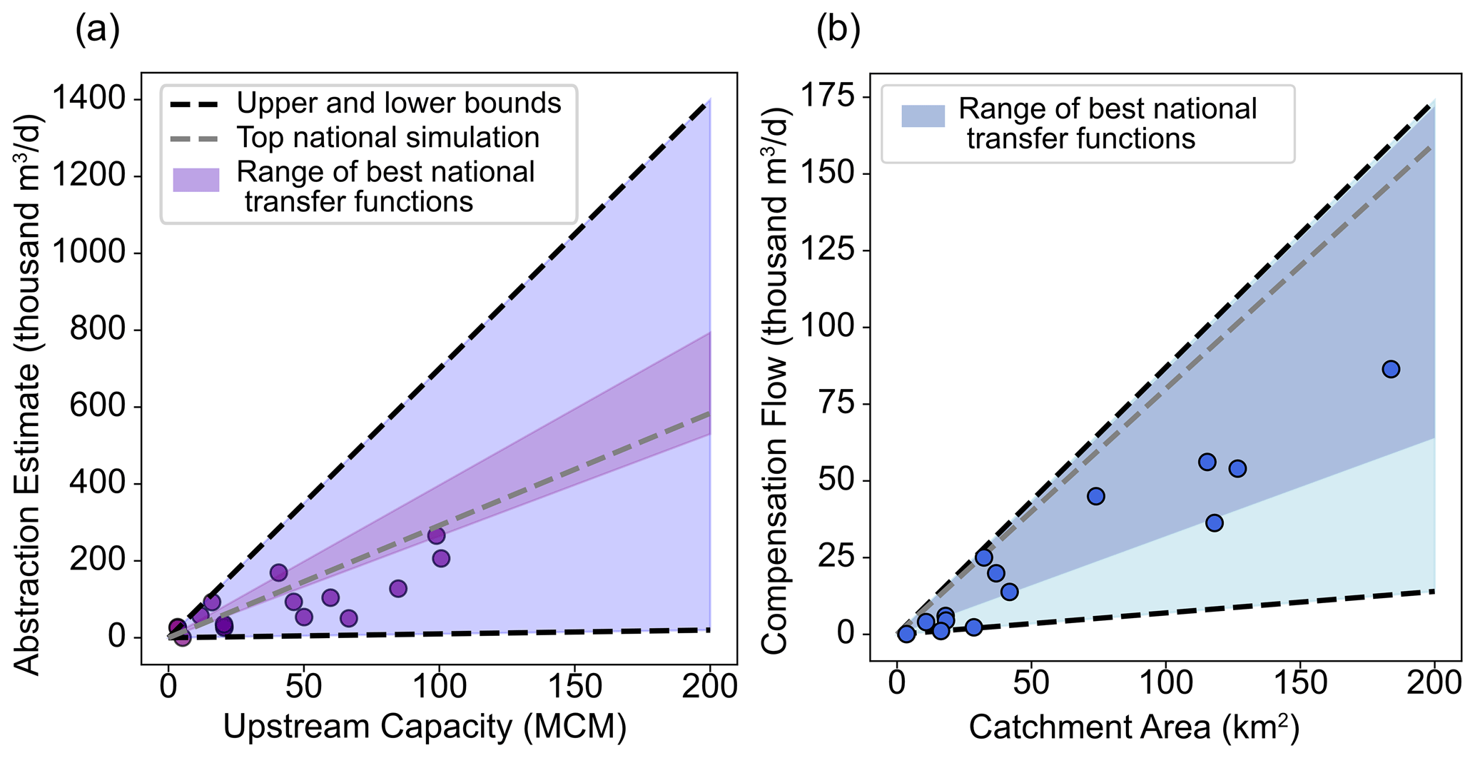
Figure 4 Relationship between (a) reservoir capacity upstream of a gauge and the reservoir abstraction volume (ABS) and (b) catchment area upstream of a gauge and compensation flow (CF). Dots represent data from a sample of catchments where abstractions could be estimated using a water balance hydrological signature and compensation flows could be extracted from drought plans, WRMPs and observed downstream flow duration curves (see Sects. 3.5.1 and S1). Dashed grey lines represent the linear transfer functions associated with the top-performing simulation from the nationally consistent calibration, the darker shading represents the spread of the top 5 % of nationally consistent simulations and dashed black lines represent the limits of the transfer function parameters based on the sensitivity of model performance to these parameters (see Supplement Table S1 and Sect. S2).

Table 1 Range of variability of the transfer function parameters (p) for use across GB. Upper and lower bounds have been determined to prevent parameter values from becoming unrealistic, whilst being as wide as possible to enable the feasible parameter space to be fully sampled.

4.3 Model evaluation (reservoir catchments)

After running DECIPHeR both with and without reservoir representation across GB, we produced 5000 flow simulations with reservoir representation and 10 simulations without reservoir representation in 205 reservoir catchments.

The following results have been split into two sections. The first (Sect. 4.3.1) presents the results from a catchment-by-catchment calibration, identifying the optimum set of transfer function parameters in each catchment (considering there are two calibrated transfer function parameters and 205 catchments, this approach identifies 410 parameters). The second section (Sect. 4.3.2) presents the results from a nationally consistent calibration (a total of two transfer function parameters assuming the same relationship between catchment and reservoir attributes in every catchment).

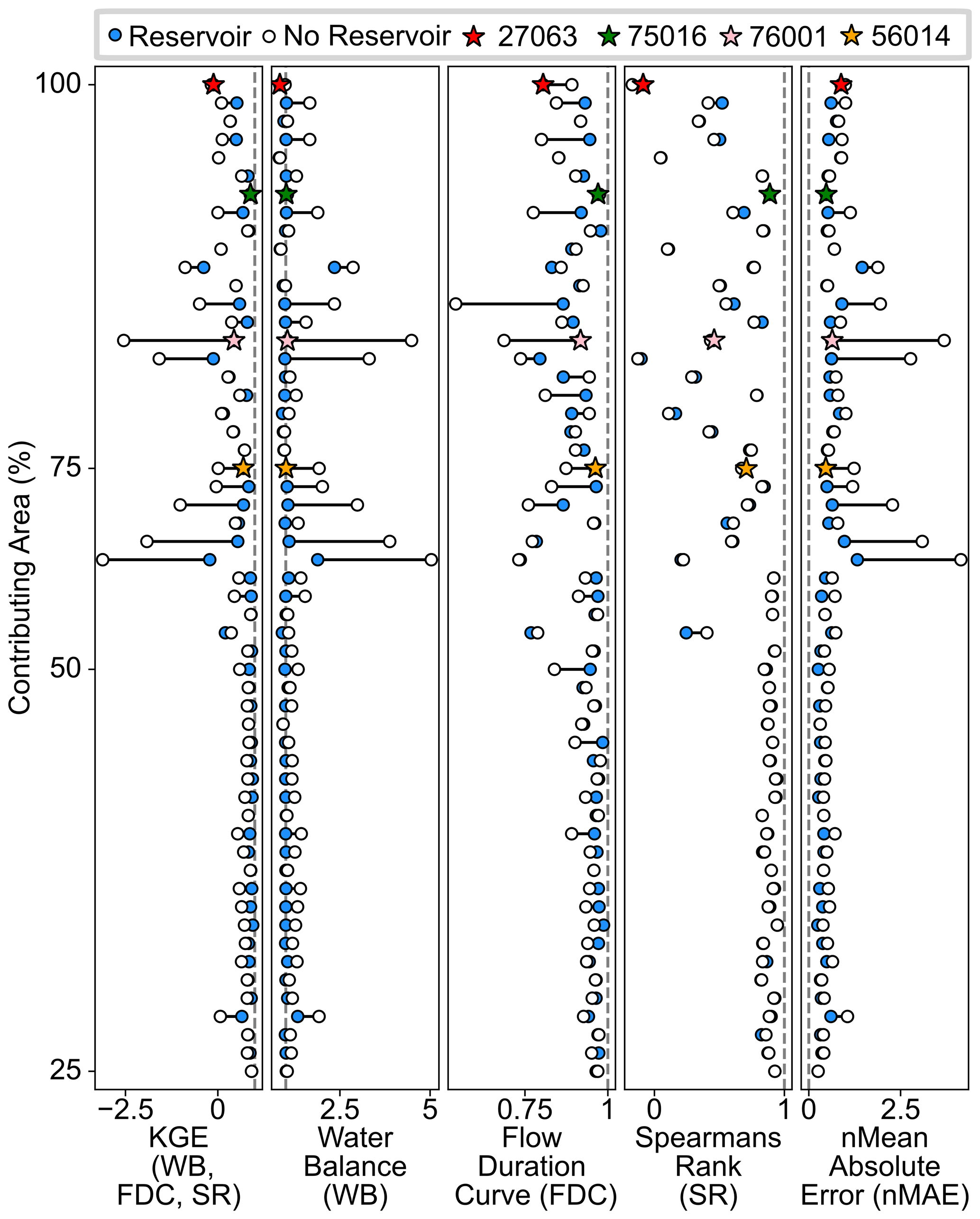
Figure 5 Difference in performance between the top reservoir simulation in each catchment and the top no-reservoir simulation. Results are presented for the non-parametric KGE metric and its relative components as well as the normalized mean absolute error (nMAE). Catchments are ordered based on their contributing area (proportion of the catchment that is drained through a reservoir). Dashed grey lines represent the optimum value for each metric; points falling closest to these lines have the best performance. Four catchments are highlighted using star markers and investigated in more detail in Sect. 4.4.

4.3.1 Top individual simulations (catchment-by-catchment calibration)

Figure 5 shows the maximum improvement in non-parametric KGE and its respective components for the top-performing simulation at all gauges downstream of a reservoir with a contributing area higher than 25 % (for full results, see Sect. S3). Figure 5 also highlights four catchments with star markers which are designed to demonstrate where the operating rules are working well and where improvements are needed (see Fig. 2 for the location of these catchments across GB). Catchments 76001 and 56014 (pink and yellow stars) show large improvements in the KGE where the operating rules are working well. Comparatively, changes in the KGE at catchments 27063 and 75016 are minimal. This is discussed in more detail in Sect. 4.4. The plot also displays an alternative to the Spearman rank correlation metric: the normalized mean absolute error. We find that for gauges with a contributing area below 25 % (of which there are 157, not displayed in Fig. 5), only nine (or 5 %) of the gauges show a non-parametric KGE improvement of more than 0.1. Only one gauge shows a decrease of more than 0.1, which suggests that the reservoir representation is not worsening model performance in catchments where reservoirs have a minimal impact. Since such a small percentage of each of these catchments is controlled by (or drained through) a reservoir, we do not expect reservoir representation to make a large difference here and exclude them from the analysis and plots below.

Of the 55 gauges with a contributing area higher than 25 %, 51 have a higher non-parametric KGE when the model includes reservoir representation compared to a model without it. Also, 28 (of 55) gauges have a non-parametric KGE increase of more than 0.1, 18 have a non-parametric KGE increase of more than 0.3, 11 have a non-parametric KGE increase of more than 0.5 and 6 have a non-parametric KGE increase of more than 1. The median change in KGE is +0.11 and the mean is +0.38. The largest improvement in KGE is 2.99, which is seen at the Haweswater Beck at Burnbanks (76001) (denoted by a pink star in Figs. 2 and 5–8), where the metric increases from −2.55 to 0.44, largely driven by the water balance component which decreases from 4.49 to 1.04. The largest decrease in KGE is −0.16 at the St Neot at Craigshill Wood (48009), which is largely driven by a decrease in the correlation component of 0.16. The median KGE across all gauges with a contributing area exceeding 25 % rises to 0.82 from 0.58 after the inclusion of reservoir representation. When you consider gauges with a contributing area higher than 50 % and 75 %, respectively, the median KGE is slightly lower but sees a larger improvement, rising to 0.55 from 0.20 pre-reservoir representation and 0.5 from 0.11 pre-reservoir representation. All gauges with a KGE improvement of more than 0.6 have a contributing area exceeding 65 %.

In general, the largest improvements in KGE tend to come from the water balance and flow duration components of the metric, and the smallest come from the correlation component. This component appears to be very insensitive to the inclusion of reservoir representation. We find that where compensation flow dominates a hydrograph, Spearman's rank cannot appropriately rank so many similar data points, and these flow plateaus contain very similar data points with large differences in ranks (see Sect. S6 and the discussion in Sect. 5.3). As a result, we calculated several other correlation-based metrics. Of these, we chose the normalized mean absolute error (nMAE) to be displayed in the Results section. Compared to the RMSE or Pearson's correlation, this metric does not put as much emphasis on the high flows (which in many reservoir catchments do not dominate much of the flow regime), and unlike the Spearman's rank, this metric can process many data points of a similar value, suitably evaluating the ability of a model to recreate the compensation flow. Reductions in the nMAE appear to be correlated with reductions in the water balance.

4.3.2 Top overall simulation (nationally consistent calibration)

Figure 6 shows the improvement in non-parametric KGE and its respective components for a nationally consistent calibration at all gauges downstream of a reservoir with a contributing area higher than 25 % (for full results, see Sect. S4). Of the 55 gauges with a contributing area higher than 25 %, 38 have a higher non-parametric KGE when the model includes reservoir representation compared to a model without it. Also, 27 (of 55) gauges have a non-parametric KGE increase of more than 0.1, 12 have a non-parametric KGE increase of more than 0.3 and 9 have a non-parametric KGE increase of more than 0.5. The largest improvement in KGE is 2.78, which is seen at gauge 76001 (denoted by a pink star in Figs. 2 and 5–8), where the metric increases from −2.55 to 0.23. The largest decrease in KGE is −0.35 at gauge 54081. The median KGE across all gauges with a contributing area exceeding 25 % is 0.73, an increase from 0.56 without reservoir representation. When you consider gauges with a contributing area higher than 50 % and 75 %, the median KGE with reservoir representation drops to 0.37 (increasing from 0.17 pre-reservoir representation) and 0.29 (increasing from 0.10 pre-reservoir representation), respectively.

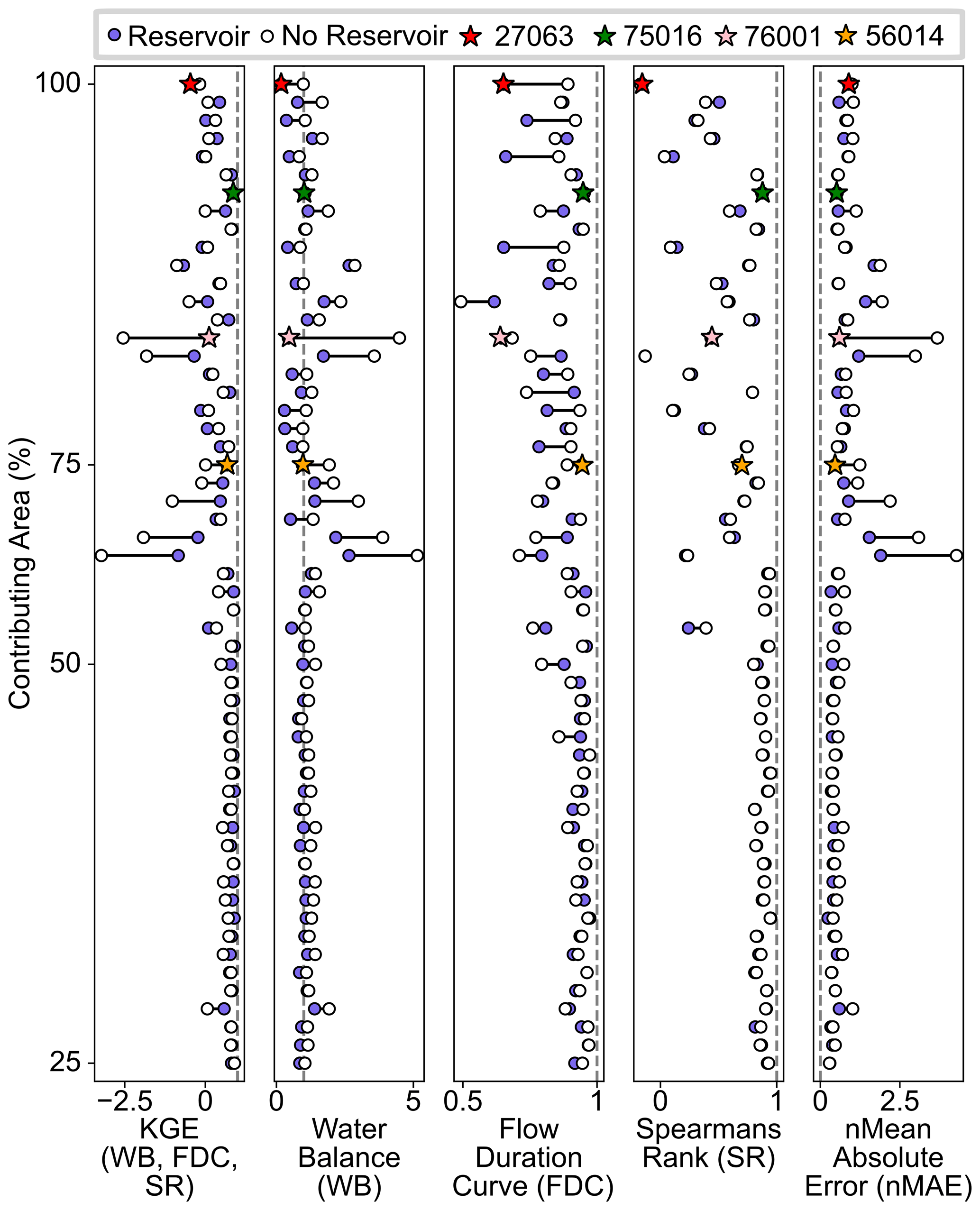
Figure 6 Difference in performance between the nationally top reservoir simulation and the nationally top no-reservoir simulation. Results are presented for the non-parametric KGE metric and its relative components as well as the normalized mean absolute error (nMAE). Catchments are ordered based on their contributing area (or proportion of the catchment that is drained through a reservoir). Dashed grey lines represent the optimum value for each metric; points falling closest to these lines have the best performance. Four catchments are highlighted using star markers and investigated in more detail in Sect. 4.4.

When using a nationally consistent calibration, there are 17 catchments where model performance decreases after including reservoir representation. Of these, eight have a decrease in KGE exceeding 0.1. In general, these are catchments where the model with no reservoir representation captures the water balance well, but when the reservoir representation forces an abstraction, this component of the KGE significantly decreases and usually decreases the flow duration curve metric too. These catchments appear to function differently from the rest of the sample, where abstractions are not taken directly from the reservoir and where releases are controlled by a different set of rules. Overall, the correlation component of the KGE shows very minimal change between reservoir and no-reservoir simulations (which is contrary to visual changes in the correlation of hydrographs).

4.4 Example reservoir catchment simulations

4.4.1 Top individual simulation (catchment-by-catchment)

Simulation results for the Usk at Usk Reservoir (56014) (yellow star) and the Haweswater Beck at Burnbanks (76001) (pink star) in Fig. 7 demonstrate some of the central improvements made by the new reservoir operating rules. Peaks seen in the no-reservoir model (without reservoir representation) are not seen (or are decreased) in the model with reservoir representation (where reservoirs are absorbing peaks in inflow by increasing storage), allowing for compensation flow to dominate the flow duration curve and hydrograph. Both gauges, 56014 and 76001, see large improvements in the KGE (0.01 to 0.69 and −2.55 to 0.44, respectively), which are largely facilitated by the improvements in the water balance and FDC components. The correlation (Spearman's rank) component of the metric has only a very small increase at both locations (56014 sees an increase from 0.67 to 0.69 and 76001 from 0.43 to 0.45) despite visually having a much more representative hydrograph. This highlights some of the problems with calculating Spearman's rank on data with little variability. The storage simulations in these two catchments follow a broadly yearly pattern of drawdown and refill. By comparing storage time series simulated at Haweswater (the reservoir upstream of 76001) to local-level data (from the Hydrology Data Explorer; https://environment.data.gov.uk/hydrology/explore, last access: 9 September 2024), we can see that the broad patterns in the simulated storage match the observed data well (see Sect. S7).

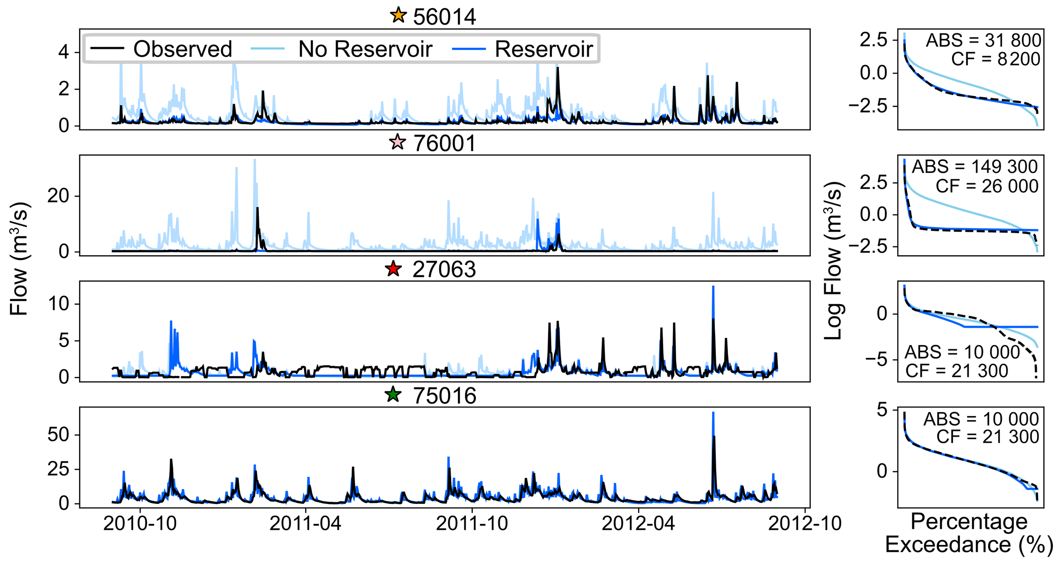
Figure 7 Hydrographs and flow duration curves from the best individual simulations (catchment-by-catchment) for selected reservoir catchments. CF and ABS are recorded on each catchment's flow duration curve in m³ d⁻¹.

Unlike the first two examples, the newly included reservoir representation does not substantially improve the KGE at the Dibb at Grimwith Reservoir (27063) (red star) (KGE increases from −0.18 to −0.11). The reservoir located in this catchment plays a central role in regulating downstream flow which is not anticipated by our simple rules. The routine releases can be seen in the observed hydrograph, but since these play a different role to the compensation flow and are instead pulses of water intended to maintain downstream flow, they are not recreated by our simple rules. The ABS parameter here is very low to account for the fact that there are no abstractions, but even this small abstraction decreases the water balance component of the non-parametric KGE from 0.98 to 0.83. Finally, the Cocker at Scalehill (75016) (green star) provides an example of a location where the reservoir outflow is generally unregulated. The reservoir in this catchment (Crummock Water) is very small and is full for most of the simulation (see Sect. S7), meaning the outflow is largely un-impacted and thus can be well recreated by both the simulation without the reservoir and the simulation with the reservoir.

4.4.2 Top national simulation (nationally consistent)

Results with the nationally consistent calibration (Fig. 8) show similar differences between simulations with and without reservoirs in catchments 56014 (yellow star) and 76001 (pink star). Peaks in the no-reservoir simulations are absorbed by the reservoirs, and compensation flow dominates much of the hydrograph. At gauge 76001, the ABS parameter has increased from 149.3 in the catchment-by-catchment simulation to 247.7 with a nationally consistent calibration. This abstraction is likely to be much higher than reality and explains the decrease in the water balance to 0.44 (compared to 1.04 in the catchment-by-catchment results). However, this still brings the metric much closer to 1 than the no-reservoir simulation which achieves a value of 4.49. Both of these catchments are relatively insensitive to changes in the CF parameter. The increase in the ABS parameter in both of these catchments is reflected in the simulation of reservoir storage (see Sect. S7 for reservoir storage simulations). These reservoirs (particularly Haweswater reservoir upstream of gauge 76001) are much more consistently drawn down in the nationally consistent simulations.

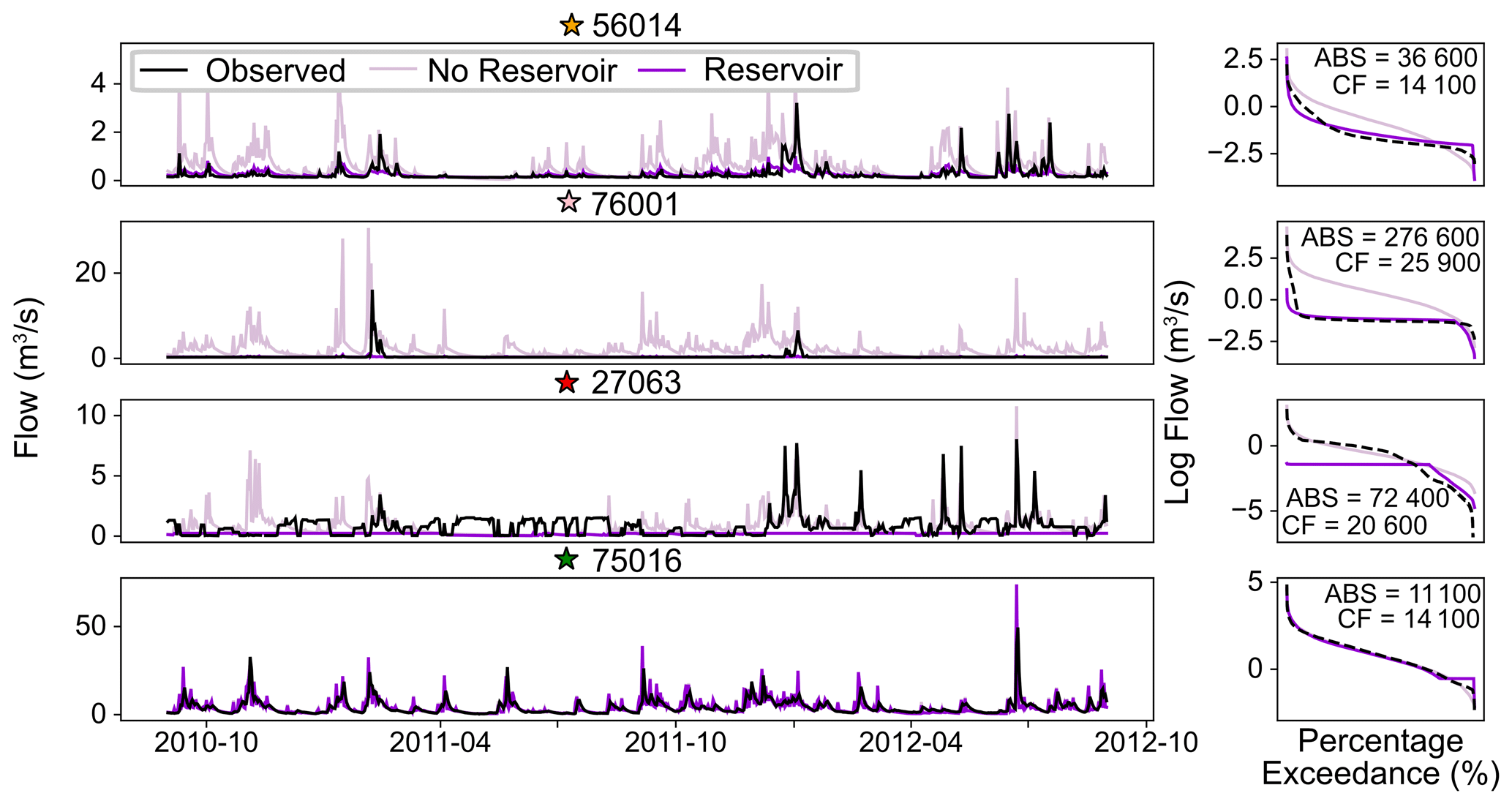
Figure 8 Hydrographs and flow duration curves from the best median simulation (nationally consistent calibration) for selected reservoir catchments. CF and ABS are recorded on each catchment's flow duration curve in m³ d⁻¹.

A similar over-abstraction is also seen in catchment 27063 (red star), where the nationally consistent calibration enforces a daily abstraction of 648 000 m³ d⁻¹, meaning that since the reservoir is never full (and never spills) the compensation flow dominates the hydrograph. Here, enforcing the nationally consistent transfer function parameters reduces the non-parametric KGE from −0.18 to −0.42. Most of the performance loss here comes from the water balance component, followed by the flow duration curve. Finally, the model performance remains very constant at gauge 75016 (green star). This is because, despite the enforced abstraction, the reservoir still remains full for the majority of the simulation. In this catchment, the KGE remains at 0.86 across the reservoir and no-reservoir simulations from the best catchment-by-catchment and nationally consistent calibrations, and it is insensitive to the reservoir parameters.

Finally, Sect. S8 reports a comparison of the top nationally consistent simulation with the widely used Hanasaki rule (Hanasaki et al., 2006) in this selection of catchments. Although the Hanasaki rule has no calibrated parameters and is therefore arguably simpler than ours, we found that it delivers a much poorer performance. This is largely because the Hanasaki rule does not allow for abstraction from the reservoirs, which is a key component of reservoir operation in most GB reservoirs.

5 Discussion

5.1 Can we improve model performance with simple operating rules?

After integrating a set of simple operating rules into a national-scale hydrological model, we found that large gains in model performance are possible with only two additional calibrated parameters. The best results were produced when these parameters were calibrated at each downstream gauge, but amongst reservoirs with a single purpose (water supply), a nationally consistent calibration can also make significant improvements.

The improvements we have achieved in simulating streamflow with reservoir representation are similar to others seen in the literature (Turner et al., 2020; Yassin et al., 2019; Coerver et al., 2018). However, what makes this study unique is twofold. Firstly, it is the simplicity of our operating rules. Many of the alternative sets of calibrated reservoir operating rules introduced in the literature have far more calibrated parameters than the two we have introduced here (e.g. Yassin et al. (2019) recommend six parameters that are determined for every month of the year, leaving 72 total parameters; Turner et al. (2021) introduce a data-driven scheme with 19 parameters). Most of these rules are, to some extent, attempting to recreate specific operating policies or rule curves and by extension introduce significant additional complexity compared to our flux-based approach. A second key advantage of our operating rules is their minimal data requirement. It is not uncommon for a set of reservoir operating rules to require storage, inflow and release data to calibrate their parameters, which are rarely available over large scales (Yassin et al., 2019; Turner et al., 2020; Ehsani et al., 2017). Contrastingly, our rules (which only require a reservoir's location, capacity and catchment area) ought to be more transferable to large-scale modelling, particularly in regions where inflow, outflow and storage time series are unavailable (such as GB).

To our knowledge, this is also the first time water supply reservoirs have been the focus of a large-scale study. Unlike hydropower (Abeshu et al., 2023) or irrigation (Hanasaki et al., 2006) reservoirs, water supply reservoirs are rarely the focus of large-scale studies, despite the fact that 22 % of reservoirs globally (according to the GRanD database) play a role in water supply. Instead, in many uncalibrated models, this type of reservoir is often collated into one “non-irrigation” category (Hanasaki et al., 2006; Wisser et al., 2010). In this case, reservoir rules usually aim to (where possible) release mean flow at all times of the year or reduce intra-annual variability. Since these rules facilitate no abstractions or compensation flow requirement, we consider them unsuitable for most of the reservoirs in our sample. Although we have only tested our approach at water supply reservoirs, a similar set of transfer functions and simple rules could be designed to suit reservoirs of other purposes. While we do not expect our rules to outperform more complex approaches, our rules provide a simple and practical starting point as a benchmark for incorporating reservoir representation into hydrological modelling where, due to data limitations, none of the pre-existing approaches can be applied.

5.2 Can we identify a nationally consistent calibration?

Overall, a nationally consistent calibration across most of the reservoirs in our sample worked well, where 49 % of gauges (with a contributing area higher than 25 %) saw the non-parametric KGE increase by more than 0.1 after the inclusion of the nationally consistent operating rules. This is promising given this approach uses only two parameters (compared with 410 in the catchment-by-catchment approach) and open-access catchment and reservoir attributes, thus reducing computational requirements (where a model no longer needs to be calibrated in every catchment) and facilitating the application of our operating rules to ungauged basins or to reservoirs located in countries with fewer data available for calibration. We find that, within our sample of reservoirs, catchment area and reservoir capacity are reasonable predictors of the compensation flow and abstraction volume across most water supply reservoirs.

There are very few examples of calibrated operating rules which undertake a similar nationally consistent calibration. Yassin et al. (2019) introduce rules which may be applied in a similar, nationally consistent manner, but the parameters are extracted from inflow, storage and release data which are not available in GB (or many other locations). Turner et al. (2021) extrapolate their rules to data-scarce reservoirs, but the calibration varies from location to location and rules are fitted to observed data. We suggest that our approach can act as an informative lower benchmark (Seibert et al., 2018) to compare to more complex approaches that involve more detailed calibration, more parameters or higher data requirements.

However, while the nationally consistent calibration worked well for many of the reservoirs in our sample, there were some catchments where a nationally consistent calibration did not work well, particularly those which contained reservoirs fulfilling multiple purposes or regulating downstream flow. Although we included only reservoirs classified as water supply reservoirs (from the UK Reservoir Inventory) in our sample, in practice some of these reservoirs fulfil multiple objectives (e.g. Cow Green Reservoir plays a role in flood management, and Kielder Water is used for hydropower). Furthermore, approximately seven of the reservoir catchments in our sample contained upstream reservoirs which play a different role in the water supply system than the rest of the sample. In these locations, reservoirs focus on facilitating downstream abstractions (rather than those taken directly from the reservoir). It is no surprise that our rules do not work well here, where they are likely to miss some crucial coordination with the downstream river and misrepresent the purpose of the reservoir (Rougé et al., 2021). However, future work might consider defining new transfer functions to describe the operating rules at reservoirs in this sample (see Sect. 5.4 for more detail).

5.3 Metrics to evaluate reservoir-impacted time series

Although much of the literature assessing reservoir operating rules evaluates their success with metrics such as RMSE (or nRMSE) (Turner et al., 2020), KGE (both parametric and non-parametric) (Yassin et al., 2019) and Nash–Sutcliffe efficiency (NSE) (Voisin et al., 2013), we advise that this is interpreted and carried out with caution.

Standard metrics such as the non-parametric KGE worked well in our near-natural catchments; however, when used to evaluate reservoir-impacted hydrographs, their shape and distribution meant that the correlation component of the metric was not informative. The Spearman's rank was not able to characterize correlations between two time series with low variability (i.e. when the compensation flow dominates the regime), which is often the case in reservoir-impacted time series. Although the Spearman's rank was chosen for the non-parametric KGE over the Pearson correlation for its lower sensitivity to extreme values and focus on mean and low flows (Pool et al., 2018), in many reservoir-impacted catchments it was this portion of the hydrograph which the metric could not evaluate properly.

Although several other metrics were tested to look at the timing, or correlation, of our simulated flow, these were often very influenced by the high flows. Whilst matching the timing of these high flows is an important component of simulating reservoir-impacted flows, we were interested in where a reservoir absorbed a peak in inflow (releasing only the compensation flow) or spilled in broadly the right week/month rather than on the exact day. The Pearson correlation and RMSE put too much emphasis on the daily peaks, giving more weight to larger errors. Comparatively, the nMAE was less influenced by the peaks in flow and large errors, providing a better evaluation of a time series dominated by the compensation flow.

We suggest that future studies should seek to develop new signatures which replace the correlation component of the KGE evaluation metric and can better capture behaviour in human-influenced catchments (Kiraz et al., 2023). Standard metrics like the KGE should be calculated on impacted time series with caution, where their ability to evaluate natural time series does not always translate.

5.4 Limitations and future work

A limitation of this study was our inability to capture reservoir operations at gauges where upstream reservoirs fulfil multiple purposes as well as facilitating water supply. Future work might investigate whether this second cluster of multi-purpose or river-regulating reservoirs could be represented by a similar set of simple rules. By extension, national-scale inventories could benefit from sub-categories for reservoir purpose, including a multi-purpose category. Furthermore, although these rules have only been tested at water supply reservoirs in Great Britain, they may be useful for simulating reservoirs in other locations. Whilst operations will vary country by country, this simple approach could be used to design rules and transfer functions for application elsewhere. Where a nationally consistent approach is not appropriate (perhaps due to multi-purpose reservoirs or more complex coordination), transfer functions could be useful in defining the parameter bounds for calibration and establishing relationships between reservoir and catchment attributes and model parameters.

6 Conclusions

This study presents a set of new, simple operating rules designed to simulate operations at water supply reservoirs across large scales. We demonstrate their application across GB, where national-scale hydrological modelling has not previously included reservoir representation. Our approach performs well across a large sample of reservoirs, with the largest performance gains established from a catchment-by-catchment calibration. Although it performs less well, our nationally consistent calibration should act as an informative lower benchmark for simulating operations at water resource reservoirs before more complex rules are considered. The results of this study should encourage the inclusion of reservoirs in national-scale hydrological modelling across GB, since we have identified large gains in performance with minimal data and added complexity.