Simulating sub-hourly rainfall data for current and future periods using two statistical disaggregation models: case studies from Germany and South Korea

The simulation of fast-reacting hydrological systems often requires sub-hourly precipitation data to develop appropriate climate adaptation strategies and tools, i.e. upgrading drainage systems and reducing flood risks. However, these sub-hourly data are typically not provided by measurements and atmospheric models, and many statistical disaggregation tools are applicable only up to an hourly resolution.

Here, two different models for the disaggregation of precipitation data from a daily to sub-hourly scale are presented. The first one is a conditional disaggregation model based on first-order Markov chains and copulas (WayDown) that keeps the input daily precipitation sums consistent within disaggregated time series. The second one is an unconditional rain generation model based on a double Poisson process (LetItRain) that does not reproduce the input daily values but rather generates time series with consistent rainfall statistics. Both approaches aim to reproduce observed precipitation statistics over different timescales.

The developed models were validated using 10 min radar data representing 10 climate stations in Germany and South Korea; thus, they cover various climate zones and precipitation systems. Various statistics were compared, including the mean, variance, autocorrelation, transition probabilities, and proportion of wet period. Additionally, extremes were examined, including the frequencies of different thresholds, extreme quantiles, and annual maxima. To account for the model uncertainties, 1000-year-equivalent ensembles were generated by both models for each study site. While both models successfully reproduced the observed statistics, WayDown was better (than LetItRain) at reproducing the ensemble median, showing strength with respect to precisely refining the coarse input data. In contrast, LetItRain produced rainfall with a greater ensemble variability, thereby capturing a variety of scenarios that may happen in reality. Both methods reproduced extremes in a similar manner: overestimation until a certain threshold of rainfall and underestimation thereafter.

Finally, the models were applied to climate projection data. The change factors for various statistics and extremes were computed and compared between historical (radar) information and the climate projections at a daily and 10 min scale. Both methods showed similar results for the respective stations and Representative Concentration Pathway (RCP) scenarios. Several consistent trends, jointly confirmed by disaggregated and daily data, were found for the mean, variance, autocorrelation, and proportion of wet periods. Further, they presented similar behaviour with respect to annual maxima for the majority of the stations for both RCP scenarios in comparison to the daily scale (i.e. a similar systematic underestimation).

1 Introduction

Urban hydrological systems are characterized by large impervious surface areas and dense underground drainage networks; therefore, their response to rainfall is direct and fast (Meierdiercks et al., 2010; Sohn et al., 2020). In such systems, rainfall events with different fine-scale temporal variability may lead to significantly different patterns of flooding (Oh et al., 2016; Dao et al., 2020a, b, 2022; Park et al., 2021) and the associated disasters such as landslides, water quality and ecosystem degradation, and risk to public health and safety. Therefore, the acquisition of fine-scale rainfall data is critical for accurate estimations, understanding the causes and impacts of floods (Berne et al., 2004; Vorobevskii et al., 2020), and thus enabling the design of sustainable and resilient urban drainage systems that can adapt to changing climate conditions.

However, fine-scale (e.g. 10 min or finer) rainfall data suitable for urban flood analysis are often unavailable. In situ gauge data are usually measured at hourly or daily intervals, due to the issues of initial cost, maintenance, data quality, and applicability; thus, available time series are sometimes still not long enough to yield reliable statistics. In addition, most future rainfall projection data produced by recent global (e.g. daily) and regional (e.g. hourly) climate models for downscaling have a coarse temporal resolution (Dyrrdal et al., 2018; Iles et al., 2020), making it difficult to precisely analyse the urban flood risks associated with climate change. Although recent climate models allowing for the explicit modelling of deep convection (Prein et al., 2015) can simulate 5 min precipitation fields (Meredith et al., 2020), these products will not be available on a large scale in the near future due to computational and data storage limitations (Schär et al., 2020).

The lack of fine-scale precipitation data can be tackled by rainfall downscaling techniques (Maraun et al., 2010). Two main approaches can be distinguished, namely, conditional and unconditional models. Conditional disaggregation models (Müller-Thomy et al., 2018) refine the temporal resolution of the original rainfall time series. Therefore, the sum of the disaggregated fine-scale rainfall contained in the original coarse time step is similar to (canonical models) or precisely the same as (micro-canonical models) the original coarse rainfall value. Unconditional models (often referred as rainfall generators), on the other hand, aim to reproduce the statistics of the original rainfall time series, rather than actual daily sums. They employ techniques such as linear regression, probability density function fitting, and machine learning to characterize rainfall processes (e.g. event depth, event duration, and inter-event time), based on which variables comprising rainfall processes are produced and superposed on an empty time axis to synthesize fine-scale rainfall time series. Therefore, unconditional models do not preserve the rainfall records of the original coarse data, but they can generate an infinite length of synthetic time series; thus, they are mainly used as the input data for the disaster risk uncertainty analysis based on Monte Carlo simulation. Like unconditional models, which are exclusively stochastic nature, conditional models also can include stochastic components.

While many conditional (Koutsoyiannis and Onof, 2001; Kossieris et al., 2018; Lombardo et al., 2017; Müller and Haberlandt, 2015; Müller-Thomy, 2020) and unconditional (De Luca and Petroselli, 2021; Fatichi et al., 2011; Papalexiou, 2018; Pidoto and Haberlandt, 2023; Peleg et al., 2017; Semenov and Barrow, 1997; Verdin et al., 2018) models have been developed, only very few studies address models that can produce fine-scale (e.g. finer than 30 min) rainfall data. Licznar et al. (2011) developed a conditional model based on a random cascade. They introduced a unique scale-dependent cascade coefficient to produce fine-scale (5 min) information to improve the model performance with respect to reproducing the fine-scale rainfall depth distribution as well as key statistics such as the mean and standard deviation of the annual rainfall maxima. Lombardo et al. (2017) proposed a conditional model that simulates rainfall time series with a given dependence structure, wet/dry probability, and marginal distribution at a finer timescale, preserving full consistency with variables at a coarser parent timescale. The suggested model was tested on 30 min rainfall data from Viterbo, Italy, and accurately reproduced the marginal distributions of the characteristic variables of both fine- and coarser-scale rainfall time series as well as the correlation structure, intermittency, and clustering. The conditional model of Kossieris et al. (2018) combines the Bartlett–Lewis process to generate rainfall events with adjusting procedures to modify the low-resolution (i.e. hourly) variables so as to be consistent with the high-resolution (i.e. sub-hourly) variables. The suggested model successfully replicated important statistical properties up to a 5 min scale at a wide range of timescales, including an improved fit for the intensity- and duration-dependent internal rainfall structure, skewness, extremes, and dry proportions, compared with its predecessor (Koutsoyiannis and Onof, 2001). Another conditional model of Müller and Haberlandt (2018) combined a trifurcation and bifurcation random cascade method to obtain a 5 min rainfall time series. The method was tested on the 24 gauges of Lower Saxony, Germany, and showed improved performance with respect to reproducing regular statistics and extremes as well as sewage system behaviour compared with the conventional bifurcation-based cascade models. Park et al. (2021) suggested an unconditional model that is also based on the Bartlett–Lewis process. They modified the original model structure, which assumes a rectangular rain cell shape, to a sinusoidal rain cell shape; thus, the model can produce the 5 min rainfall given hourly rainfall input. The 5 min rainfall data synthesized by the modified model contained more realistic extreme rainfall values as well as flooding behaviour in urban environments compared with the model assuming a rectangular rain cell structure.

In spite of this progressive evolution of fine-scale rainfall downscaling models, most studies have focused on the development of a single model or on validating existing models of the same kind at multiple study sites (D. Kim et al., 2013, 2016, 2017; Takhellambam et al., 2022; Wang et al., 2021). Only a few studies have performed a comparative analysis of multiple disaggregation models, as undertaken in this work. Pui et al. (2012) compared three typical types of conditional models (i.e. a random multiplicative cascade model, a point process model, and a resampling model) that disaggregate daily rainfall to an hourly resolution. The comparison was performed at four point locations in Australia with different climatic regimes. They discovered that all of the models simulated the commonly used statistical measures of rainfall reasonably well at an hourly time step, the microcanonical cascade model overestimated the hourly rainfall variance, and extreme rainfall values were under- or overestimated by the cascade models. However, to date, no studies have compared conditional- and unconditional-type disaggregation models at the fine timescale resolution (10 min) critical for urban system analysis as well as for a variety of rainfall characteristics under different climatic systems.

This study aims to utilize promising techniques for temporal fine-scale downscaling of future rainfall by applying models that do not have many statistical requirements regarding the correlations of process driving variables and that are not dependent on many input datasets. Furthermore, the model application should be simple, mostly automatic, and fast.

With this overarching goal in mind, the first aim of this study is to compare newly developed conditional and unconditional models for the task of fine-resolution rainfall downscaling. The conditional model used in this work is composed of a unique, new combination of a Markov chain for simulating binary sub-daily events alignment and a copula-based sampling of actual precipitation values, which, to our knowledge, has not been attempted in our field yet. The unconditional model used in this study is an advanced version of the Poisson cluster rainfall generation model (Kaczmarska et al., 2014; Kim and Onof, 2020). It can synthesize future rainfall under climate change given a change factor (the ratio of the mean of the future to current rainfall) that can be easily obtained from climate change rainfall products. The model has a unique structure to obtain parameters for future rainfall generation that, to our knowledge, has not been tried by other studies. In addition, the two focus regions of this study cover a wide range of climate and rainfall characteristics: while both Germany and Korea have temperate climates, Germany has a more moderate and stable rainfall pattern with less regional variation (600–1800 mm yr⁻¹), whereas Korea is characterized by more regional variation with respect to its rainfall patterns and amounts (1200–2000 mm yr⁻¹) and is subject to long-lasting heavy frontal rainfall during the summer months as well as intense typhoons. Therefore, the validation of these models for this variety of rainfall characteristics should reveal the suitability and limitations of the model application in general as well as providing some insight into transferability to other regions.

One of the novelties of this study is the use of radar rainfall data instead of gauge data. In contrast to gauges, which can accurately observe rainfall depth at a point location, weather radar observes rainfall in a fine, granular format over a wide spatial range. Thus, radar data could be more suitable for understanding regional climate and its non-stationarity as well as for application to climate projection data. In addition, the chronic issue of radar rainfall measurement accuracy has been constantly addressed via various methods such as the Z–R relationship improvement (Alfieri et al., 2010; Kim et al., 2021; Kirsch et al., 2019) and radar–gauge merging (Goudenhoofdt and Delobbe, 2009; Han et al., 2021; Ochoa-Rodriguez et al., 2019; Sinclair and Pegram, 2005). Consequently radar rainfall products are being actively adopted by many studies focused on understanding hydrologic systems (Ghimire et al., 2022; Wijayarathne et al., 2020, 2021) as well as those on operational flood warning systems (Ramly et al., 2020; Liu et al., 2021). However, to our knowledge, there is only one study (Jasper-Tönnies et al., 2012) that has applied 5 min radar data and used a relatively simple “objective weather types” method to pick an observed radar event with a similar daily sum to downscale climate projection data. No other studies have investigated the applicability of recent improved-quality radar data (Park et al., 2014; Winterrath et al., 2018) to rainfall downscaling, especially based on two unique methods with contrasting traits.

A further aim of this work is to test the described models on climate projection data. Therefore, after the data were calibrated and validated for the current period, both models were employed to produce 5 min rainfall data corresponding to the Representative Concentration Pathway (RCP) 2.6 and 8.5 scenarios. The fine-scale data produced by each of the methods were compared in terms of the change factors of various statistics and annual maximum rainfall values.

The research questions discussed in this article are as follows:

1. How well do two different fine-scale rainfall disaggregation models produce data, and are they suitable for reproducing important rainfall statistics as well as extreme values?

2. What are the differences and similarities between the presented types of disaggregation models?

3. How might future fine-scale rainfall change according to the respective models?

The paper is organized as follows: Sect. 2 provides a detailed description of the models, study areas, and data sources, including both radar data and future projection data; Sect. 3 presents the results of our analysis, including a comparison of the two models and an assessment of their accuracy; finally, in Sect. 4, we summarize our findings and discuss their implications for future research as well as revenue opportunities in the field of rainfall disaggregation.

2 Methods and data

2.1 WayDown

WayDown is an automated conditional precipitation disaggregation model that was developed at the Chair of Meteorology at the Technische Universität Dresden. It is wrapped in an R package and is available on GitHub (https://github.com/hydrovorobey/WayDown, last access: 20 April 2023) along with a test dataset.

The principle scheme is presented in Fig. 1. WayDown disaggregates daily precipitation by iterating over each day and keeping the daily sums consistent. This could be station or climate projection datasets. In the first step, a precipitation event is selected using the high-resolution reference data for the desired month. To do so, all reference events with daily sums similar to the input value are subsetted. The Markov chain's two-state transition matrix is estimated from these events and is then used to sample binary (“rain”/“not rain”) 5 min precipitation time series for a given day. Thereafter, the actual precipitation heights are sampled for respective intervals with binary precipitation, which can be either single or consecutive sub-events. The first value for the sub-event is directly sampled (with empirical probability weights) from the observed data, accounting for a daily value and the respective month of occurrence. The second and following time steps with precipitation are selected based on a 2D empirical beta copula (Segers et al., 2017) constructed from the reference high-resolution dataset in a way that the subsequent precipitation height depends on the previous one, thus representing the lag-1 autocorrelation model. Afterwards, the sum of the obtained disaggregated time series is compared to the original daily input value. If the absolute difference is less than an assumed threshold (i.e. 10 %, which was found to be suitable with regard to computation time for the study sites but might be changed for other datasets), a proportional correction is applied. Higher values receive a proportionally larger correction than smaller values. For small daily precipitation sums (e.g. less than 1 mm), a higher threshold can be allowed (i.e. 100 %) to reduce the computational time. Otherwise, the disaggregation process is repeated again until a convergence error value less than threshold is reached: first, the new values are sampled for the same binary time series; second, after 30 unsuccessful attempts (default number that can be changed), a new binary time series for a given day is sampled. Finally, the framework considers day-to-day event transition, taking into account the last precipitation value from the disaggregated time series of a previous day to create a consistent event for the current day (Fig. 2) which is sampled from the obtained transition matrix using a starting value of 1 for a newly created binary time series.

Figure 1 WayDown framework algorithm.

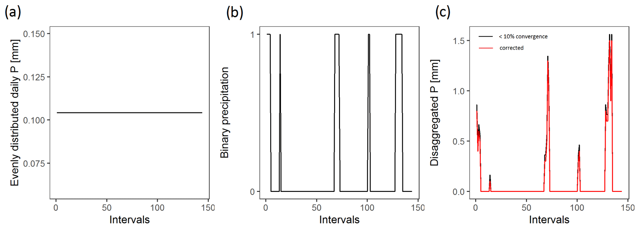
Figure 2 WayDown disaggregation example of 1 d precipitation (daily value of 15 mm, last-interval value from previous day of 0.5 mm) for Leipzig, Germany, in July using 10 min resolution radar data (144 intervals). (a) Uniformly distributed daily value (evenly disaggregated for all intervals). (b) Binary precipitation event sample considering month and daily value. (c) Sampled precipitation values for each interval and their correction to obtain the required daily sum (convergence error of 8 %).

WayDown was tested with the reference input data resolutions of 1, 5, 10, and 30 min. The model does not require substantial resources with respect to computational power, time, or memory. For example, on a 3.4 GHz, 16 GB RAM PC, the model takes approximately 1 h to disaggregate 80 years of data to a 10 min timescale using 20 years of reference radar data (see the test dataset with data for Leipzig provided along with the R package).

2.2 LetItRain

LetItRain represents an unconditional rainfall generation model and (Kim and Onof, 2020) is an upgraded version of the Poisson cluster model (Kaczmarska et al., 2014; Rodriguez-Iturbe et al., 1988). The model was developed at Hongik University's Hydrology Innovation Laboratory and is available on the lab's webpage (https://sites.google.com/site/hihydrology/projects, last access: 20 April 2023). LetItRain simulates synthetic rainfall time series, based on the assumption that storms arrive following a Poisson process, and different probability distribution functions, which define the duration of storms and the properties (arrival, duration, and intensity) of rain cells. Existing Poisson cluster rainfall generation models tend to underestimate rainfall extremes, which is why the LetItRain model incorporates the following model improvements: (1) it accounts for the fitting of the first- to third-order moments of observed rainfall; (2) the model inversely relates the rain cell duration to intensity for reproducing short-term extreme rainfall events; (3) LetItRain assumes a gamma distribution for the intensity of the rain cell; and (4) the model applies two shuffling algorithms to reproduce the autocorrelation of storms and long-lasting rainfall. With these improvements, the model is capable of reproducing observed statistical properties as well as extremes over a wide range of timescales.

The LetItRain application to simulate future sub-hourly rainfall time series is described in Fig. 3. First, rainfall statistics for each calendar month are calculated from the high-resolution reference data (i.e. radar rainfall). These statistics include the mean, variance, covariance, skewness, and proportion of wet periods for the aggregation intervals of 10, 30, 60, 120, 240, 480, and 960 min. Here, the whole time series (i.e. including dry periods) are considered. Then, regressions between obtained statistics (specified in Fig. 4a) are derived. One of them is a standard first-order linear regression, which is used for estimating the relationship between the mean and variance as well as between the mean and the proportion of wet periods. The other is the same type of regression, but without an intercept, which is used for variances at different aggregation intervals (i.e. 10 min variance vs. 30 min variance). The same procedure is repeated for the wet periods of different aggregation intervals. Second, the change factor for the mean value is calculated for a daily scale. It is defined as the ratio of the means between the historical and future periods and is used to adjust the future 10 min precipitation mean. The change factor approach is, for example, also used by the LARS-WG stochastic weather generator (Semenov et al., 1998) to generate future daily time series for impact modelling. Third, future rainfall statistics are estimated using the output of the previous two steps (Fig. 4). The mean value for the future 10 min rainfall is defined by multiplying the observed 10 min mean and the change factor. Future mean values for other aggregation intervals are derived by multiplying the 10 min mean by a fixed factor. Afterwards, the variance and proportion of wet periods for the future period are estimated using the regressions obtained for the historical data and future mean values. Future statistics for covariance and skewness are assigned directly from the reference high-resolution input dataset, as no suitable relationship between rainfall statistics was found here and the sensitivity of simulations to the variation in those statistics is weak (Fatichi et al., 2011). Although some indications exist that higher-order moments of precipitation characteristics will change in the future (Chan et al., 2016), detailed information from models is missing; thus, we adopt higher-order moments from the current climate.

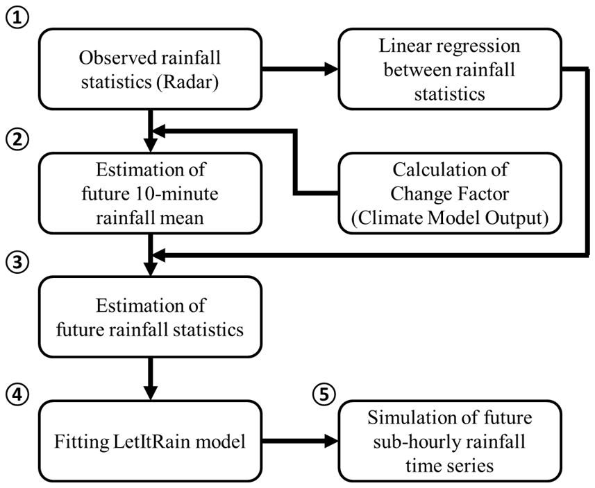
Figure 3 The procedure for the simulation of future sub-hourly rainfall time series using the LetItRain model.

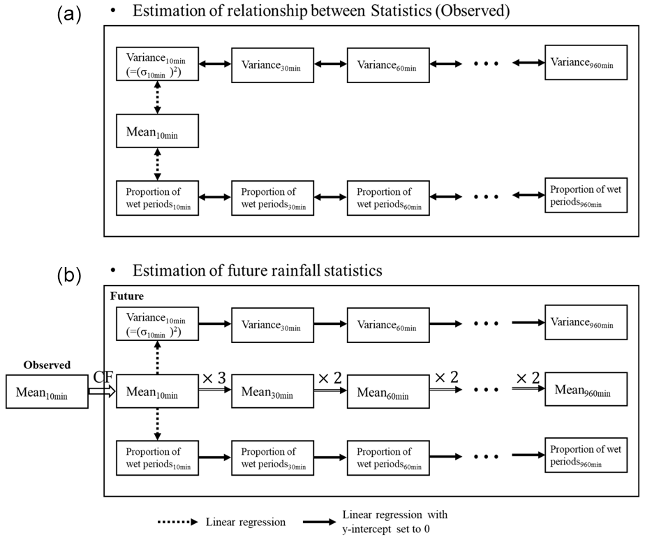
Figure 4 (a) Rainfall statistics for the estimation of the linear regression relationship. (b) The procedure for the estimation of future rainfall statistics.

Estimated rainfall statistics for the future period (mean, variance, covariance, skewness, and proportion of wet periods for different aggregation intervals) are used to calibrate the model. Finally, the future sub-hourly rainfall time series are generated using the derived model parameters. A procedure of model calibration and the calibration results are presented in the Supplement (Vorobevskii, 2023).

2.3 Precipitation data

For the case study, five locations in Germany and five locations in South Korea were chosen (Fig. 5). The German sites (Leipzig, Naumburg, Greiz, Hof, and Klingenthal) are located on plains and in low mountain ranges (in the central eastern part of Germany). They are characterized by a continental climate (Dfb – humid continental, warm summer subtype; Kottek et al., 2006) with annual precipitation sums of around 600–1000 mm. A total of 50 %–80 % of the annual precipitation falls in June–September and stems from both convective and stratiform events, whereas the total precipitation amounts are much smaller in winter and are mainly of cyclonic origin (Jung and Schindler, 2019). The Korean sites (Seoul, Gangwon, Daejeon, Gwangju, and Busan) are characterized by a continental climate (Dwa and Dfa – humid continental, hot summer subtype) with annual precipitation sums of between 1200 and 2000 mm. More than half of this amount falls during the typhoon season, during which time a stationary front lingers for about a month, in summer (June–September). Winter precipitation is typically less than 10 % of the annual sum.

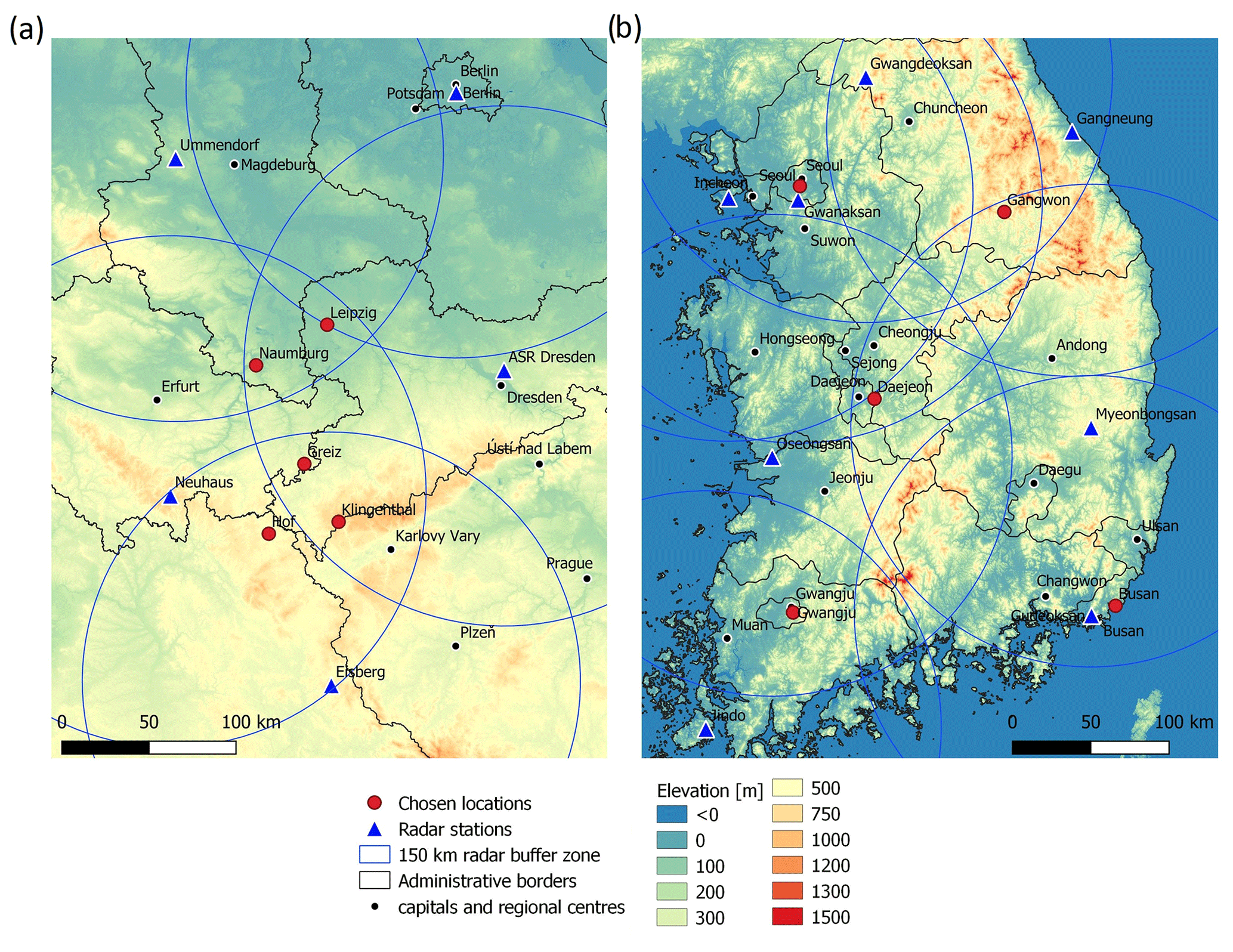
Figure 5 Overview map of the chosen locations and corresponding radar stations for (a) Germany and (b) South Korea. The background elevation map was created using SRTM30 satellite data (NASA, 2013).

Radar data were utilized as a high-resolution reference dataset. For the German sites, the Radar-based Precipitation Climatology Version 2017.002 dataset (available at https://opendata.dwd.de/climate_environment/CDC/help/landing_pages/doi_landingpage_RADKLIM_RW_V2017.002-en.html, last access: 20 April 2023) was used (Winterrath et al., 2017). The dataset is a composite available on a 1 km× 1 km grid for the time period from 2001 to 2020 at a temporal resolution of 5 min. It represents a product of the RADOLAN method, in which the precipitation sums from the radar-based precipitation estimates are adjusted using measurements from conventional gauges (Winterrath et al., 2017). Thus, for the chosen locations, data from five overlapping radar stations (Berlin, Dresden, Eisberg, Neuhaus, and Ummendorf) are merged. For sites in South Korea, the composite radar rainfall product CM1 (available at https://data.kma.go.kr/data/rmt/rmtList.do?code=11&pgmNo=62, last access: 20 April 2023) from the Korea Meteorological Administration (KMA) was used. The dataset merges observations from 11 radar stations and has a 1 km× 1 km grid with a temporal resolution of 10 min covering the period from 2009 to 2019. Observed reflectivity data are first passed through a Gaussian model adaptive processing (GMAP) filter (Siggia and Passarelli, 2004), which corrects for echoes caused by the surrounding terrain, such as beam blockage. Then, another quality control algorithm was applied that detects non-precipitation echoes, thereafter removing them based on the criterion related to the difference in reflectivity on the upper and lower side from a certain altitude (Park et al., 2014).

For the German sites, the Canadian Earth System Model (second-generation) projections (CanESM2) for the RCP2.6 and 8.5 scenarios downscaled with the EPISODES model were used for the period from 2020 to 2100. CanESM2 with a T63 (∼ 1.9^∘) resolution consists of the physically coupled CanCM4 atmosphere–ocean model coupled to both terrestrial carbon and ocean carbon models (Arora et al., 2011). EPISODES is an empirical-statistical downscaling method (Kreienkamp et al., 2019). It implements a two-step procedure. The first part provides day-by-day meteorological information at regional scales; the second part uses this information to produce synthetic time series via a weather generator. The target grid corresponds to the EURO-CORDEX resolution of 0.11^∘ (∼ 12 km). Original climate projection data with daily resolution were bias-corrected using monthly quantile mapping on the 1 km× 1 km interpolated station-based RaKliDa dataset (Kronenberg and Bernhofer, 2015).

For the Korean sites, high-resolution data from the KMA with Shared Socioeconomic Pathway (SSP) scenarios 1-2.6 and 5-8.5 (SSP1-2.6 and SSP5-8.5, respectively) covering the period from 2020 to 2100 were chosen (available at http://www.climate.go.kr/home/CCS/contents_2021/Kma_climate_RCP.html, last access: 20 April 2023). The dataset is based on the UKESM1 global model and a set of dynamic and statistical downscaling models. UKESM1, from Met Office Hadley Centre, is based on the HadGEM3-GC3.1 model (atmosphere–land–ocean–sea ice) combined with the JULES terrestrial model and the MEDUSA ocean biogeochemical model (Sellar et al., 2019). This global model has 135 km resolution that is dynamically downscaled to 25 km through the ensemble mean (Kim et al., 2022) of the five regional climate models (HadGEM3-RA, RegCM4, SNURCM, GRIMs, and WRF) participating in the CORDEX-EA II project. Finally, the regional climate model was downscaled to a 1 km grid by the PRIDE model (M.-K. Kim et al., 2016) using ground observation data and the Barnes approach (Barnes, 1964).

For all sites, the nearest grid cells to the study sites were taken from the respective datasets. For the sake of consistency between German and Korean radar datasets, the German one was aggregated to a 10 min resolution. Comparability between different climate projection generations (Climate Model Intercomparison Project phases 5 and 6 – CMIP5 and CMIP6, respectively) and, thus, between the respective RCP and SSP concepts is also preserved (O'Neill et al., 2016): RCP2.6 and SSP1-2.6 compared to RCP8.5 and SSP5-8.5.

2.4 Model validation and the evaluation of climate projections

Validation of both methods was done via the comparison of disaggregated and original radar datasets, where the former was produced using original radar values aggregated to a daily scale. Although both methods are of a stochastic nature, the straightforward comparison of the disaggregated time series of both methods is not possible, as LetItRain acts as a Monte Carlo precipitation simulator, whereas WayDown maintains daily precipitation sums that are consistent with the input data (although it implies a stochastic component). Thus, the following statistics were chosen to compare models on a monthly and annual scale for the whole and non-zero time series: the mean, the variance, the transition probabilities of the Markov chain, autocorrelation function values, the proportion of wet period, the frequency and quantiles of extreme events of various magnitude, and annual maxima. Furthermore, the 1000-year time series were generated for each station in order to test the possible variability in model simulation statistics. To do so, the WayDown model was run 50 times for the German stations and 91 times for the Korean stations with the same daily radar input for each station, so that the total length of the n-times run was equivalent to 1000 years. Thus, the differences between runs are introduced by the model event-value generation process. For the LetItRain case, the model was calibrated to station data and 1000-year time series were then directly simulated, as it is a generator model type.

Disaggregated time series of the future climate projections were evaluated with regard to change factors and annual extremes. Change factors were calculated as a simple ratio between the future and historical period for the following precipitation statistics: the mean, variance, autocorrelation function, proportion of wet period, and 99 % extreme quantile. For both disaggregation models, the same precipitation datasets were applied for each respective country. Thus, the 10 min radar dataset was used as training data to disaggregate climate projections (the two selected RCPs).

3 Results and discussion

3.1 Validation of the methods with radar data

3.1.1 Visual inspection of observed and disaggregated model events

A direct comparison of observed radar and disaggregated precipitation events using standard methods, like time series overlap plots or the correlation coefficient, is not reasonable due to the stochastic nature of the models. However, a qualitative visual mapping is possible. For that, five random daily events from typical winter (February) and summer (July) months were selected, with daily sums close to respective daily mean values (left panels in Figs. 6 and 7). Corresponding disaggregated events were randomly picked from the generated time series considering the same (or close for LetItRain) daily sums and similar daily maxima with previously chosen radar events (middle and right panels in Figs. 6 and 7).

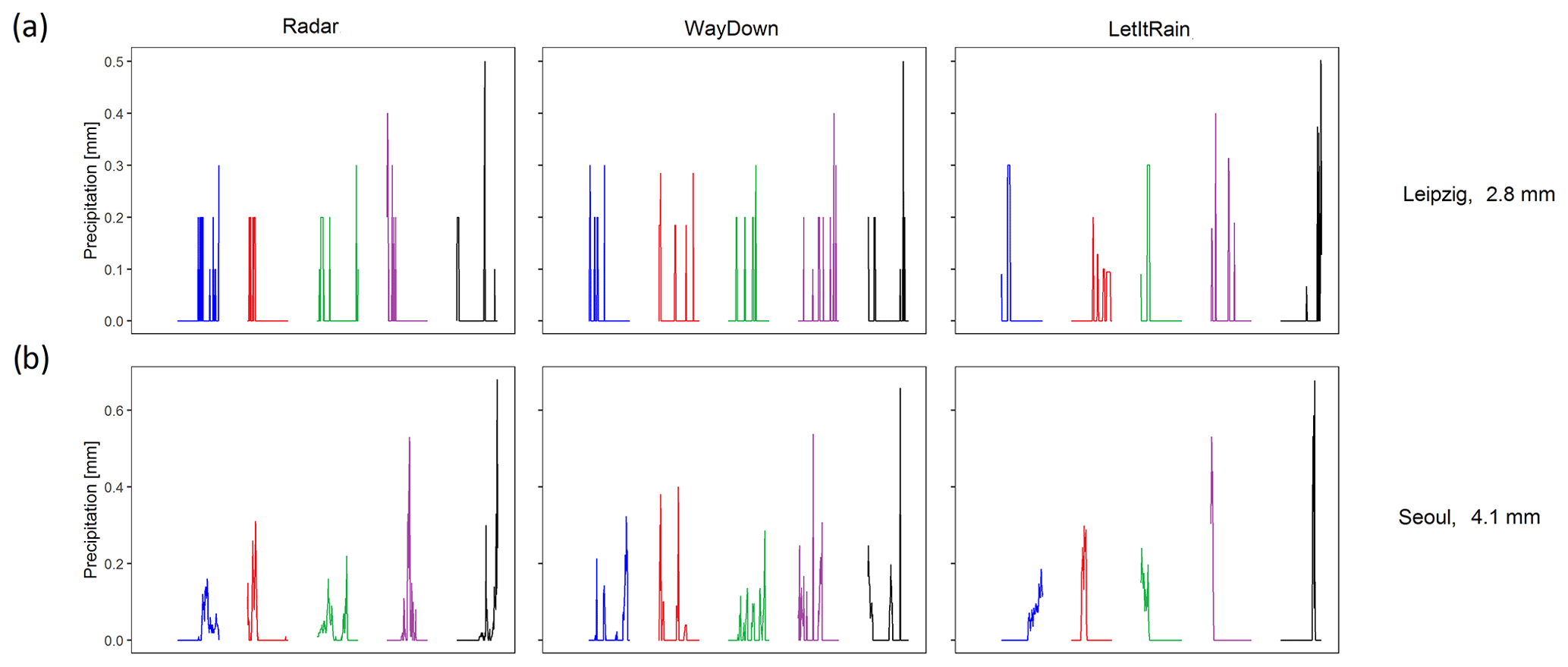
Figure 6 A total of 5 sample days with rain in winter (February) with typical daily sums for (a) Leipzig, Germany, and (b) Seoul, South Korea. Different colours represent separate days.

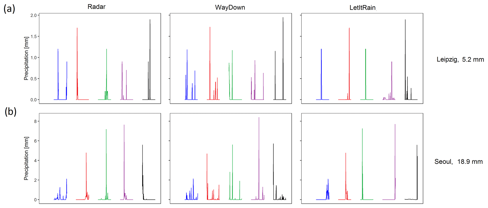
Figure 7 A total of 5 sample days with rain in summer (July) with typical daily sums for (a) Leipzig, Germany, and (b) Seoul, South Korea. Different colours represent separate days.

For Leipzig, a typical winter event has a sum of 2.8 mm and a maximum intensity of 0.2–0.6 mm over a 10 min period (upper subplot for radar in Fig. 6). In the summer time, higher values are normally observed: a 5.2 mm daily mean and maxima of 0.5–2 mm over a 10 min period (upper subplot for radar in Fig. 7). For Seoul, however, the difference between February and July is more prominent, and events are generally more autocorrelated. Typical means are 4.1 and 18.9 mm for the winter and summer months, respectively, and typical maxima range from 0.2–0.7 mm over a 10 min period in February to 1–8 mm over a 10 min period in July (lower subplots for radar in Figs. 6 and 7).

Based on visual inspection, both models show satisfactory results with respect to replicating 10 min radar data for both cities, capturing the typical magnitude, variability, and alignment of sub-daily rain events, especially considering the variability in precipitation regime, seasonality, and radar precision (middle and right subplots for WayDown and LetItRain, respectively, in Figs. 6 and 7).

3.2 Comparison of the main statistics

Validation results are presented as monthly statistics plots for Leipzig and Seoul in Fig. 8 (for other stations, see Appendix Fig. A1) and as annual statistics for all stations in Table 1. According to radar data, the mean and variance values (Fig. 8a–d) for the Korean stations were found to be 2–10 times higher than for the German stations (0.011 and 0.039 mm for the mean and 0.010 and 0.074 mm² for the variance, respectively). Transition probabilities from “dry” to “wet” conditions (Fig. 8e) are similar for both countries (0.01–0.05), while “wet–wet” persistence probabilities (Fig. 8f) for Korean locations (0.75–0.90) are slightly higher than for German stations (0.60–0.70). Autocorrelation function values (Fig. 8g–j) were also found to be higher for Korean sites. For example, for a 10 and 60 min lag, the monthly variance between autocorrelation values was found to be 0.5–0.75 and 0.15–0.35 for Germany and 0.60–0.80 and 0.20–0.50 for South Korea, respectively. Typical proportions of wet periods (Fig. 8k) for Korean stations lie between 13 % and 19 %, whereas German stations showed much lower values (3 %–4 %), which is in line with the differences in frontal precipitation behaviour for the two countries.

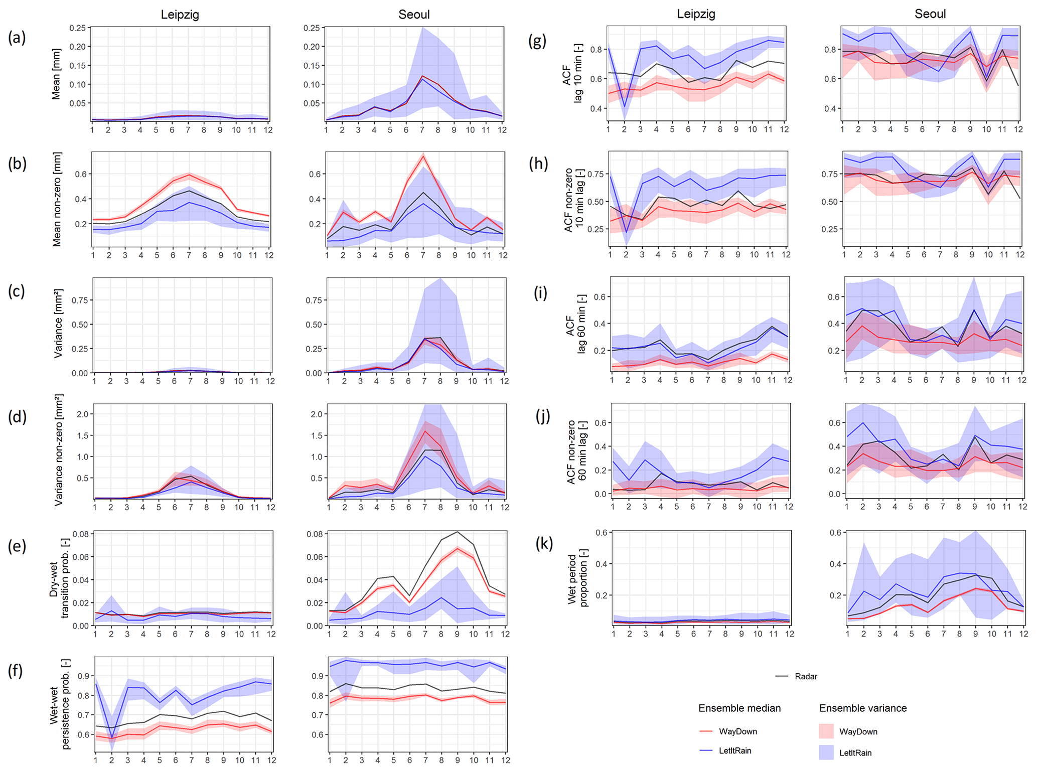
Figure 8 Comparison of monthly statistics between disaggregated and original radar data for Leipzig and Seoul.

Statistical moments of the first and second order for the full time series length were well represented by both LetItRain and WayDown. This includes not only the values of the annual mean and variance but also replication of the pronounced seasonal cycle. Only minor deviations for both models were observed, mostly for the summer months. A perfect match between the precipitation mean values for radar and WayDown can be explained by the nature of the method, as it keeps the daily sums consistent. However, the difference between the models' behaviour is noticeable for the non-zero time series. WayDown overestimates the non-zero mean by 0.05–0.4 mm for both countries, especially in summer months (Fig. 8b). This is consistent with the simultaneous underestimation of dry–wet period proportions while keeping the daily sums preserved, and it can be explained by two reasons. The first reason is the systematic overestimation of sampling from the fitted 2D empirical copulas, which apparently do not possess a good representation of the real precipitation behaviour. Secondly, the assumed 10 % convergence to the daily sum of the disaggregated values used for the final adjustment procedure could be too high and needs to be reduced for more precise estimations. However, this will lead to a considerable increase in the computation time. LetItRain, on the other hand, generally underestimated the non-zero mean by 0.05–0.1 mm for both countries. This can be explained by the model fitting process, which is trained to replicate the mean of observed rainfall and does not consider the non-zero mean statistics. Non-zero variance, in contrast, was better represented by both methods than non-zero means, although with the same general behaviour for both methods.

Monthly variations in Markov chain transition probabilities from dry to wet and the persistence of wet states were better modelled by WayDown, which was expected, because transition matrices were directly incorporated in the method for the binary time series sampling. However, systematic 5 %–10 % underestimations for dry–wet and wet–wet states probabilities were found for all stations. This is probably due to the shortcomings and assumptions of the radar sub-daily event subset procedure (which was used to fit the Markov chain) in WayDown based on a certain daily precipitation sum and month. Namely, the number and representativity of this subset is directly limited by the radar time series length and, thus, has a significant influence on the accuracy of transition matrix estimations. LetItRain showed multidirectional performance (both under and overestimations appeared) and generally did not replicate this statistic well including seasonality. It showed significant underestimations of dry–wet transitions and overestimations of persistence probabilities for almost all stations. Specifically, a huge mismatch was found for persistence probabilities. Although dry–dry and wet–wet transition probabilities are included in the Poisson cluster rainfall model (Cowpertwait et al., 1996), they are estimated with analytical equations based on the proportion of dry periods at several aggregation intervals. In this study, however, this parameter was not calibrated.

Autocorrelation function values of different lags were simulated by both methods with different qualities for both countries. WayDown showed a good match for a 10 min lag for non-zero time series (Fig. 8h); however, the correlations were underestimated with larger lags, which is especially noticeable for Korean sites. This is due to the incorporation of only 2D, rather than higher-dimensional, copulas for precipitation sampling, which indirectly affects the autocorrelation of higher orders. Systematic underestimation of autocorrelation for the full time series (0.1–0.3) in WayDown (Fig. 8g, i) probably originates from the underestimation of zero-precipitation intervals (proportion of wet period). LetItRain, on the other hand, better depicted the full time series and higher lags while overestimating (for German stations) or missing the annual cycle (for Korean stations) in the lag-1 autocorrelation values. The fact that LetItRain directly incorporates autocorrelation parameters of several lags in the model set-up explains the better model match. The model, however, could not be fitted perfectly for that statistic, as greater weight is set to the mean and variance compared with the autocorrelation (see the Supplement). Non-zero autocorrelation followed the full time series values with slightly worse performance for both models.

The proportion of wet periods for South Korea was underestimated by WayDown (by approximately 5 %), whereas LetItRain showed good agreement. For the German stations, WayDown showed minor underestimations (< 1 %), whereas LetItRain generally overestimated the proportion by 1 %–3 %. For WayDown, the systematic errors are connected to the problem of binary time series sampling discussed above and are directly explained by minor underestimations of dry–wet transition probabilities, which were also slightly higher for the Korean sites. In the case of LetItRain, the minor deviation occurred because the model was not calibrated to perfectly reproduce the proportion of wet periods.

Overall, based on the variety of the analysed statistical characteristics, it could be concluded that LetItRain delivers much higher variability for all variables compared with WayDown, especially for Korean stations. As LetItRain represents a rain generator, rather than a conditional disaggregation model (as is the case for WayDown), it naturally shows a wider ensemble variability. Furthermore, as the model requires the fitting of multiple statistical parameters, it was found that the calibration procedure struggled to find optimal parameters for a few stations and months (i.e. see the non-zero mean value and the proportion of wet periods for June in Leipzig), probably due to the high precipitation variability and shortage of reference radar time series.

Table 1 Summary of annual statistics for the disaggregated and original radar data.

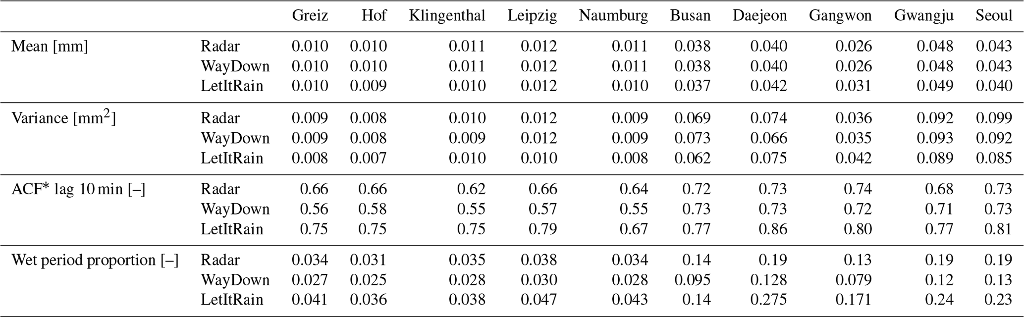
^* ACF: autocorrelation function.

3.3 Representation of extremes

Along with the replication of monthly and annual statistics, it is also important for downscaling models to maintain the consistency of extreme precipitation frequencies and magnitudes. Here, we did not account for event separation; thus, both characteristics of extremes (frequency and quantiles) were calculated from the whole time series length (for both radar and disaggregated data). This approach is also commonly found in the literature with regard to disaggregation models validation, along with event-separation and peak-over-threshold extreme analysis (e.g. Takhellambam et al., 2022; Kossieris et al., 2018). Another reason for not splitting the time series using methods such as event-based maxima or peak-over-threshold is the limited length of the observation time series. Application of these methods to estimate extreme quantiles can lead to even higher uncertainty.

Absolute frequencies of 10 min precipitation extremes for reference radar and disaggregated datasets in Leipzig and Seoul, normalized to the number of events overshooting a given threshold per 100 years, are presented in Fig. 9 (left panels). Here, a normalization to 100 years does not refer to the return period; rather, it was done to normalize the calculated frequencies for the two countries due to the different time series lengths, thereby allowing us to compare the results. Due to the differences in climate, extreme frequencies in the intensity interval from 5 to 15 mm in Seoul are 5–50 times higher than for Leipzig. For example, the estimated frequency of events with rainfall of 10 mm over a 10 min period at German sites is in the range of 15–35 per 100 years, whereas values of 155–620 per 100 years are found for sites in South Korea (Fig. A2). For all of the German sites, both models behaved in a similar way. The ensemble median of frequencies until 2–3 mm over a 10 min period is overestimated by up to 20 %, whereas it is underestimated for higher threshold frequencies, with increased magnitude towards higher values. It is noteworthy that, although it showed a slightly higher underestimation of the frequencies for the median, the LetItRain ensemble bandwidth covered zero relative difference with radar data for all German stations and intervals (right panels in Fig. 9 and Fig. A2). For the Korean stations, WayDown showed a similar over- or underestimation of extremes around the threshold of 2–5 mm over a 10 min period. LetItRain behaved differently for each Korean site, although it generally depicted lower deviations from radar data than WayDown.

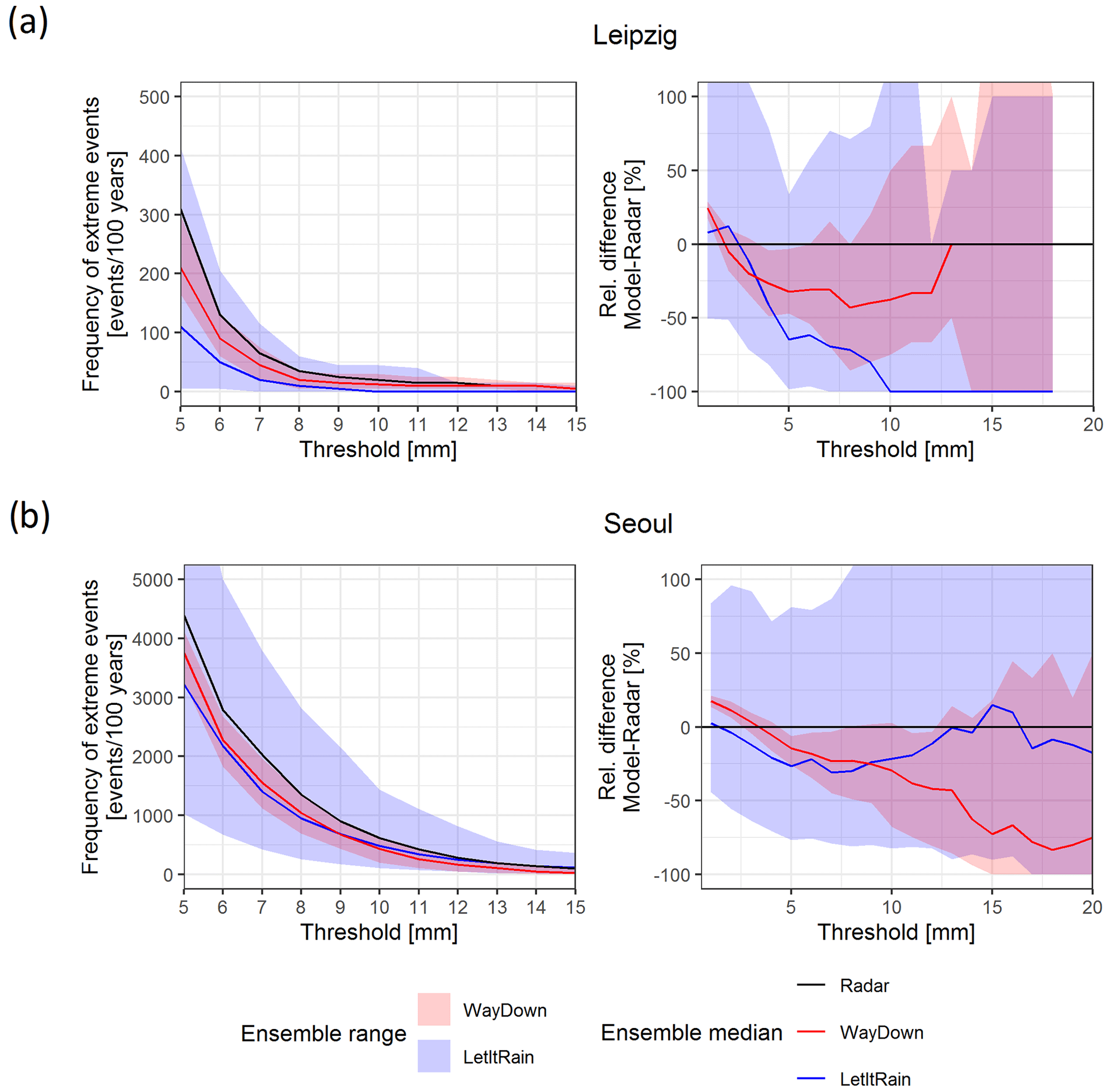
Figure 9 Absolute and relative difference in the frequency of extreme precipitation for original and disaggregated radar data for (a) Leipzig and (b) Seoul.

Extreme precipitation quantiles (0.99–0.99999) for reference radar and disaggregated datasets for Leipzig and Seoul are presented in the left panels of Fig. 10 (other stations are shown in Fig. A3). For example, estimated empirical 10 min quantiles with 0.99 probability for German and Korean sites lie in approximately the same range: 1.8–2 and 2.1–3.1 mm, respectively (Fig. A3). These results look plausible with regard to the difference in climate and time series lengths. For the German stations, WayDown overestimated extreme quantiles until 0.99–0.999 probabilities, thereafter producing slight underestimations with deviations of approximately 20 % from the observed data. LetItRain, on the other hand, showed a good fit on extreme quantiles up to the 0.99 percentile and underestimations for higher percentiles. For the stations in South Korea, WayDown overestimated extremes up to the 0.999 percentile, thereafter underestimating them with deviations of up to 40 %. LetItRain showed a slight underestimation of quantiles, except for Busan. Similarly to extreme frequencies, LetItRain showed a much wider ensemble bandwidth with errors of up to 100 % for rare events (right panels in Fig. 10).

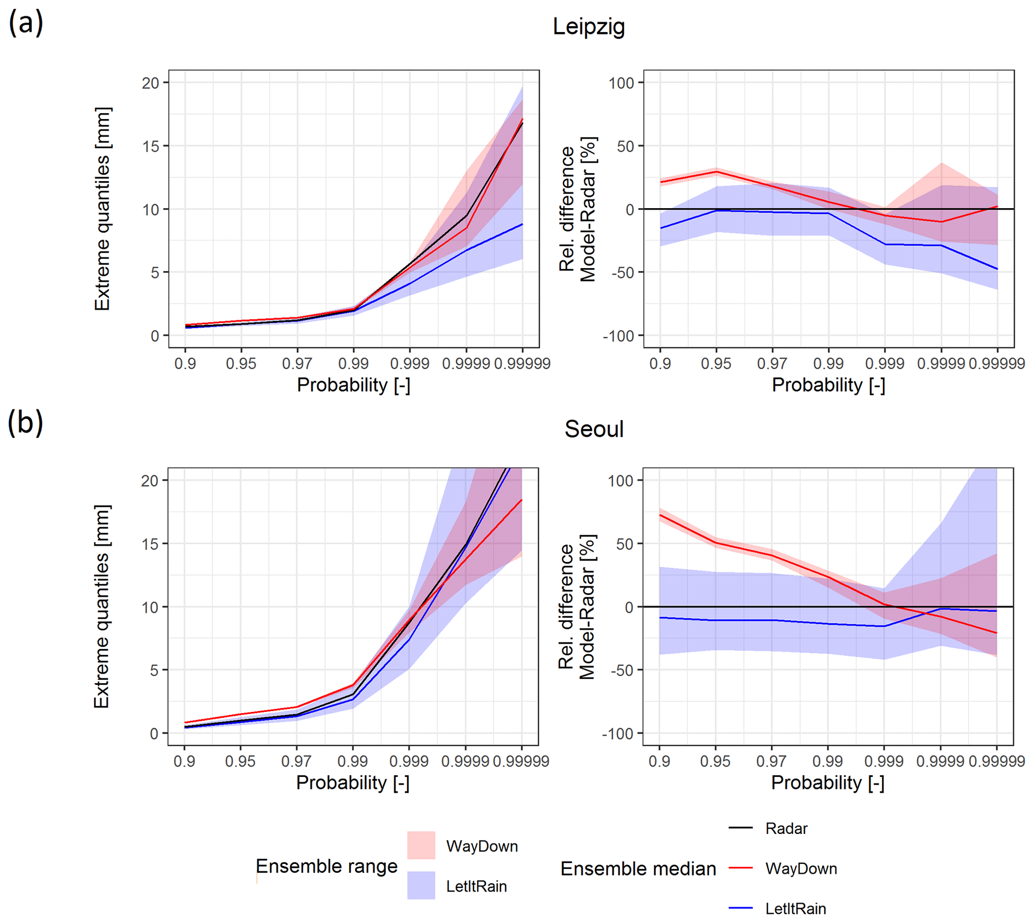
Figure 10 Absolute and relative difference in extreme precipitation quantiles for original and disaggregated radar data for (a) Leipzig and (b) Seoul.

The variability in the annual maximum precipitation for reference radar and disaggregated datasets for all stations is shown in Fig. 11. According to radar data, the median annual maximum values for German sites are 6.3–7.5 mm over a 10 min period, whereas typical maximum values are almost twice as high for the Korean locations (10.9–15.0 mm over a 10 min period). For all German stations, plots show systematic underestimation of annual maxima for both models. The distributions for all 1000-year-equivalent time series depict higher positive skewness, and median values of 4.9–5.9 mm over a 10 min period for WayDown and 4.3–5.5 mm over a 10 min period for LetItRain were found. On the other hand, no systematic underestimation was noticed for the stations in South Korea. Simulations from LetItRain were closer to radar data, with median values of 10.0–16.8 mm over a 10 min period, whereas WayDown showed deficient agreement (median of 7.7–12.8 mm over a 10 min period).

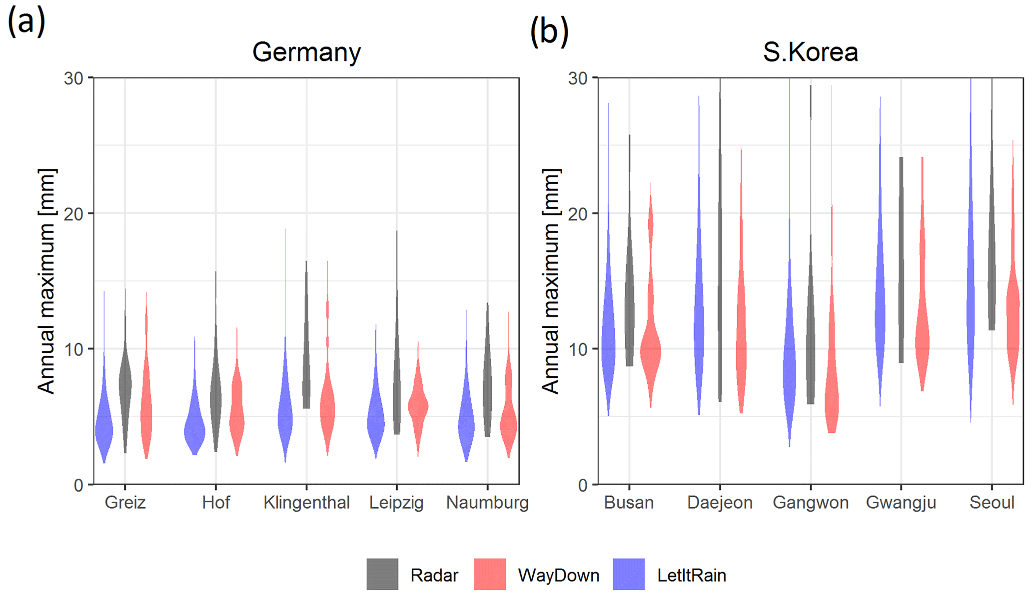
Figure 11 Violin plots with annual 10 min precipitation maxima for original and disaggregated radar data for (a) Germany and (b) South Korea.

The problems with the WayDown approach shown above regarding the representation of the extremes (over- and underestimation of frequencies and quantiles around certain thresholds and underestimation of annual maxima) originate from the precipitation sampler, which is based on 2D empirical copula. While serving as a simple and non-site-specific universal method that does not require calibration, it showed satisfactory and robust results regarding the main statistics but naturally revealed a number of shortcomings, one of which is inaccuracy in the extreme precipitation representation. This issue (in addition to those mentioned in the previous section) can be solved via the application of improved copula sampling. Nesting copulas might improve autocorrelation, while the application of parametric copulas will provide a better fit for extremes. This, however, will lead not only to an increase in computation time but also to the challenges of a better copula family choice and fitting procedures, which are currently tricky to implement in an automatic way without user intervention and control.

The mismatch with respect to the extremes in the LetItRain results can be explained by the shuffling algorithm of the model. The model first simulates rainfall using a Poisson cluster-based rainfall model and then uses an algorithm to rearrange the rainstorms (see the Supplement; Vorobevskii, 2023). The model considers the correlation between the rainstorms in the observed rainfall and calibrates the “deg” parameter accordingly. This means that storms are more likely to be rearranged in the following fashion: storms with a greater rainfall amount flock together in a 1000-year simulation. As we segmented the generated time series into several ensembles, storms with large extreme values are likely to belong to only a few ensemble members, thereby leading to an imbalanced distribution of extremes between the ensembles.

3.4 Change factors between radar and climate projections

Change factors for the main statistics between climate projections and radar data for two scales are presented in Fig. 12. Change factors for the German stations on a daily scale showed mostly positive trends for both RCP scenarios, except for Leipzig and Naumburg, where trends were multidirectional. Korean stations, on the other hand, were mainly characterized by negative trends, except for autocorrelation, for which change factors were found to be positive for all sites.

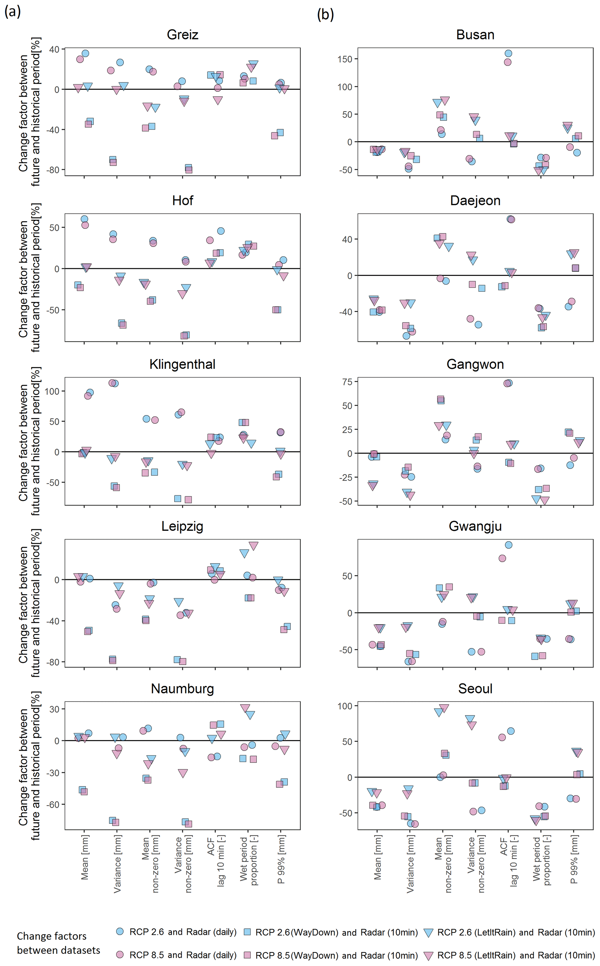
Figure 12 Change factors for the main statistics between climate projections and radar data on a daily and 10 min scale for (a) Germany and (b) South Korea.

It might be expected that the change factors from disaggregated time series of climate projections will follow a similar trend to those at a daily scale. They are based on basically the same input data as those used for the calculations of daily factors (upscaled radar and disaggregated climate projections). Moreover, the LetItRain method directly incorporates change factors scaled to a daily resolution for application to climate projections (although only for the mean). It was found that the difference in change factors between scales is much higher than between the two RCP scenarios (for the same model). Furthermore, the agreement between both 10 min datasets is higher than for the daily-scale data. Nevertheless, the direction of the trend for the daily scale was in a better agreement with 10 min data for Korean sites, compared with the German stations, simulated with both models, especially when analysing the mean, variance, and proportion of the wet periods. Only three German sites showed similarities between scales and only for a few statistics (autocorrelation and proportion of the wet periods).

For all German stations, both models resulted in a non-existing or negative trend for the mean and variance (for both the full and non-zero time series), whereas they showed mostly positive trends for the autocorrelation and proportion of wet periods. Further, extreme precipitation of 99 % was simulated differently by the methods. For Korean stations, models ended up with negative trends for the mean and variance as well as the proportion of the wet period, whereas change factors for the non-zero mean and variance as well as extreme precipitation increased for the future period. Trends in the autocorrelation did not agree between the methods. Finally, it was found that WayDown delivered lower change factors than LetItRain, especially for German locations. It should be noticed that different results from the studied disaggregation methods for the two countries could also be driven by the difference in the input daily climate projection data, due to the different disaggregation schemes of global to regional climate datasets.

Cross-analysis of the disagreement between the two scales of change factors and the problems of both methods revealed and discussed in the validation section does not show clear patterns in the context of countries nor statistics. Thus, the identified trend differences between daily and 10 min scales could not be solely explained by the shortcomings of the methods. Furthermore, as both models showed similar behaviour with respect to change factors for most of the sites and statistics, both can express the possible reality of the future precipitation changes at the finer scale.

3.5 Extremes in climate projections

We compared the behaviour of the annual maxima for all stations on a daily (Fig. 13a) and 10 min scale (Fig. 13b) to indirectly check the plausibility of the extremes in the generated time series for the climate projections. To do so, the whole length of the available time series was used (80 years for climate projection data and 20 or 11 years for radar data for the respective German and Korean stations). As in-depth discussion of the trustworthiness and quality of input precipitation climate model data is not the topic of the study, we just state here that daily-scale radar data showed significantly higher maxima than both climate model outputs for all Korean sites and two German stations (Leipzig and Naumburg). Hence, the differences in extreme statistics between the two countries could be introduced not only by the climate differences but also by the various data time series' lengths. The differences between the two scenarios are generally minor: 7 out of 10 stations deliver a slightly higher median of the annual maxima for the RCP8.5 scenario, whereas the values are similar for the remaining 3 stations. Variability in the maxima, expressed as the distance between the main quartiles (25 %–50 %), for the radar data is up to 3 times (1.5 times for German sites) higher than for the climate projections. Between the two scenarios, RCP8.5 possesses higher interquartile variability for the majority of stations.

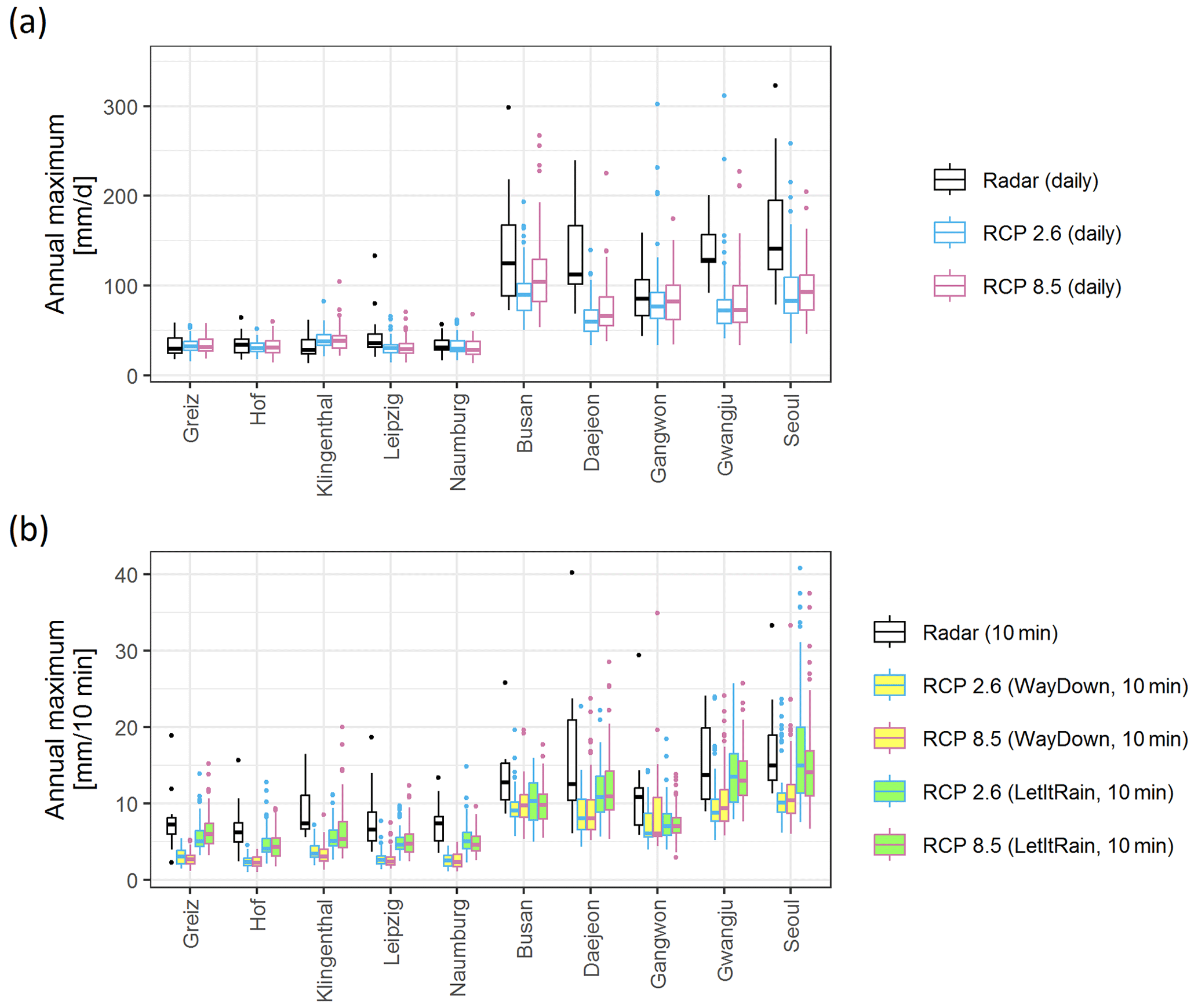
Figure 13 Annual maxima of climate projections and radar data at a (a) daily and (b) 10 min scale for Germany and South Korea.

At the 10 min scale, the median annual maxima from radar datasets exceeded those from climate projections for all stations except Gwangju and Seoul, where medians from the RCP8.5 scenarios have similar values. This is mainly driven by the underestimation of extremes in the original daily climate projection data. Except for a few cases, both LetItRain and WayDown showed similar behaviour regarding the relative differences between radar data and the RCP scenarios of disaggregated climate projections (median and variance) compared to daily data. Comparison between RCP scenarios for the same disaggregation model did not show systematic patterns, e.g. that RCP8.5 will deliver higher annual maxima, which agrees with the results at the daily scale. Comparing the two models, LetItRain delivered higher variability and noticeably higher absolute values for six stations (four Korean and two German), which could not be referred to as a systematic disagreement between two methods. This difference is also backed up by the fact that LetItRain acts as a rain generation model and already showed much higher variability between model realizations in the validation part. Thus, it could demonstrate the same feature for the 80-year-long climate projection time series, and taking an ensemble rather than one realization can narrow the inconsistency in annual maxima representation between two methods.

4 Conclusions and outlook

In this study, we presented and discussed two different methods to disaggregate the daily output of projected precipitation data to a sub-hourly scale. Although both techniques are rainfall disaggregation models, the first is a conditional model that keeps daily sums consistent (WayDown), whereas the second represents an unconditional model (rain generator) that mainly focuses on the replication of time series statistics (LetItRain). Indeed, no studies have undertaken testing of different types of disaggregation models at fine temporal scales, specifically at the 10 min interval. The outcome of such a comparative analysis provides valuable insights into the selection of an appropriate rainfall disaggregation model.

We validated both models using radar data from 10 stations located in Germany and South Korea. It should be mentioned, however, that both models are not limited to this resolution and can reproduce statistics at a resolution of up to 1 min if respective reference data are provided. The success of the validation was evaluated via the matching of multiple statistics calculated from the original 10 min radar data and disaggregated time series, for which the same upscaled daily radar data were used as model input. To account for possible model uncertainty, the disaggregation procedure was replicated several times in order to get a 1000-year-equivalent ensemble output. With regard to the ensemble median, WayDown showed better results for the monthly mean and variance (including the non-zero time series), transition probabilities of the Markov chain, 1-lag autocorrelation, and proportion of wet period, sometimes over- or underestimating the absolute values but following the sub-annual cycle. LetItRain better replicated autocorrelation values of higher lags (up to 60 min) and depicted good results for the mean and variance. Although some other characteristics on the annual scale proved to be properly simulated, the model struggled to fit the seasonal course for many statistics. Furthermore, ensemble variations in LetItRain were found to be several times higher than in WayDown. Both methods showed better results for German sites compared with Korean stations. The frequency of extremes was generally underestimated by the models for thresholds of 2–3 and 2–5 mm for German and Korean sites, respectively. For the German stations, WayDown overestimated extreme quantiles up to 0.99–0.999 probabilities, thereafter showing slight underestimations, whereas LetItRain demonstrated an underestimation of all percentiles. For the stations in South Korea, both methods overestimated extremes up to the 0.999 percentile, thereafter underestimating them.

Further, we applied the models to climate projection data and compared change factors and extremes to radar data between two timescales. For the majority of the cases, change factors for daily and 10 min resolutions do not follow each other. In fact, they depicted similar values for the same model and RCP scenario. Consistent positive and negative trends, confirmed jointly by models and daily data, were found for three stations in Germany (for autocorrelation and proportion of wet periods) and five stations in South Korea (for mean, variance, and proportion of wet periods), respectively. Both models showed similar quantile values of the annual maxima for the majority of the stations for both RCP scenarios in comparison with the daily scale. A systematic underestimation of the annual 10 min maxima was found for both methods compared with radar data. Mainly, this is due to the underestimation in the original daily climate projection data. Finally, the application of the disaggregation models to the climate projection data should be done with caution, especially if statistics of the current period are preserved and assumed for the future. Although some indications of the possible changes in sub-daily statistics exist (Meredith et al., 2019), there is still not enough consistent knowledge to prove it (e.g. high-time-resolution climate projection simulations).

The comparison of the two methods clearly revealed both similarities and differences that can provide crucial information regarding the choice of a disaggregation model type for producing fine-scale future rainfall, which few studies have yet addressed. Moreover, as was shown and discussed in the validation and application section, the presented models have the potential for improvement, which will most likely result in a higher-quality disaggregation. For WayDown, this includes the incorporation of parametric nested copulas in the precipitation sampler as well as the consideration of change factors between radar data and climate projections at the daily scale to apply these trends in the disaggregation process. For LetItRain, additional statistics can be included in the calibration procedure (e.g. transition probability). Further, the effect of skewness at a fine timescale in the calibration procedure should be investigated more deeply for the accurate replication of extreme rainfall. Moreover, a proper relationship between high-order moments of rainfall was not presented. Thus, current (historical) statistics for covariance and skewness were directly used as future statistics for model calibration. Non-linear models such as neural networks could be a solution for developing the relationship, thereby leading to the development of a model that accounts for a change in high-order moments of precipitation characteristics in the future. Moreover, future high-resolution climate model projections will be able to generate data, allowing for the deduction and incorporation of higher-order moment statistics into the presented disaggregation models. Finally, integration of methods that account for spatial correlation and, thus, allow for a shift from the point to spatial scale will be beneficial as well. Lastly, in order to prove the utility of simulation approaches, a downstream application of simulated data in urban hydrological models would also be beneficial.

Appendix A

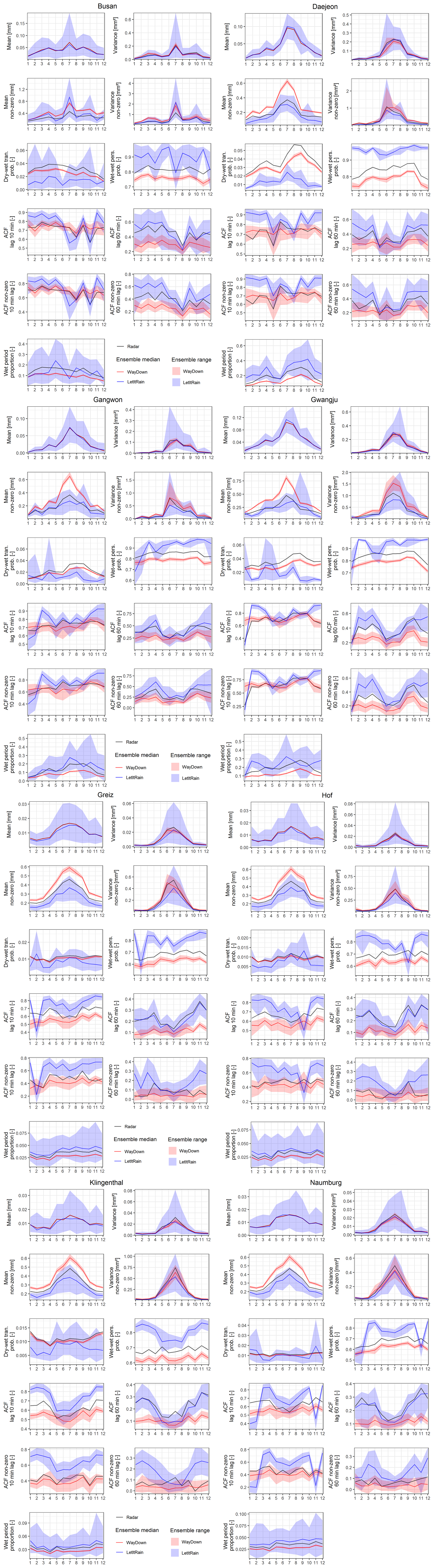
Figure A1 Comparison of monthly statistics between the disaggregated and original radar data (remaining stations).

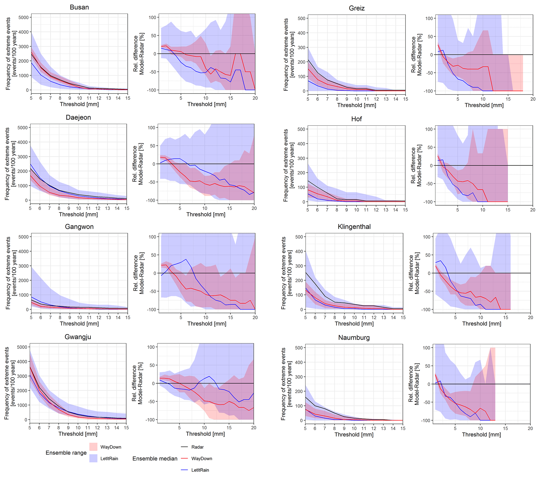
Figure A2 Absolute and relative difference in frequency of extreme precipitation for the original and disaggregated radar data (remaining stations).

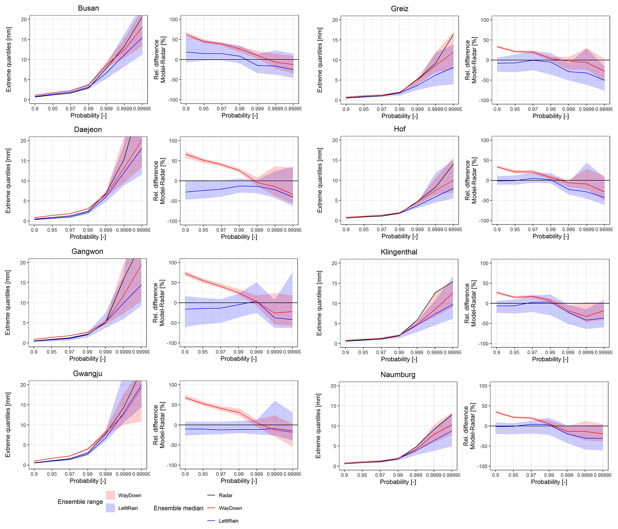
Figure A3 Absolute and relative difference in extreme precipitation quantiles for the original and disaggregated radar data (remaining stations).