the Creative Commons Attribution 4.0 License.
the Creative Commons Attribution 4.0 License.
 | 13 Aug 2024
Technical Note: The divide and measure nonconformity – how metrics can mislead when we evaluate on different data partitions
Martin Gauch
Frederik Kratzert
Grey Nearing
Jakob Zscheischler
The evaluation of model performance is an essential part of hydrological modeling. However, leveraging the full information that performance criteria provide requires a deep understanding of their properties. This Technical Note focuses on a rather counterintuitive aspect of the perhaps most widely used hydrological metric, the Nash–Sutcliffe efficiency (NSE). Specifically, we demonstrate that the overall NSE of a dataset is not bounded by the NSEs of all its partitions. We term this phenomenon the “divide and measure nonconformity”. It follows naturally from the definition of the NSE, yet because modelers often subdivide datasets in a non-random way, the resulting behavior can have unintended consequences in practice. In this note we therefore discuss the implications of the divide and measure nonconformity, examine its empirical and theoretical properties, and provide recommendations for modelers to avoid drawing misleading conclusions.
- Article
(2232 KB) - Full-text XML
-
Supplement
(702 KB) - BibTeX
- EndNote


Measuring model performance is a foundational pillar of environmental modeling. For instance, in order to ensure that a model is suited to simulate the rainfall–runoff relationship, we have to test how “good” its predictions are. Hence, over time, our community has established a set of performance criteria that cover different aspects of modeling. We use these criteria to draw conclusions with regard to the evaluation and the model. Therefore, criteria should exhibit consistent behavior that follows our intuitions. However, when we use these criteria it is important to keep in mind that each one has specific properties – certain advantages and disadvantages – that are relevant for interpreting results.
The Nash–Sutcliffe efficiency (NSE; Nash and Sutcliffe, 1970) is the perhaps most used metric in hydrology. In this contribution we show that the NSE exhibits a counterintuitive behavior (which, as far as we can tell, is so far undocumented), captured by the following exemplary anecdote. A hydrologist evaluates a model over a limited period of time and obtains an NSE value of, say, 0.77 (Fig. 1, blue partition). Then, a large event occurs and an isolated evaluation for that specific event results in the slightly worse model performance of, say, 0.75 (Fig. 1, orange partition). One might then expect that the overall performance (i.e., a model evaluation over both the blue and the orange partitions) should be bound by the values obtained during evaluation over each partition separately. However, the NSE over the entire time series in this example is 0.80 (Fig. 1, purple partition), which is higher than either partition.
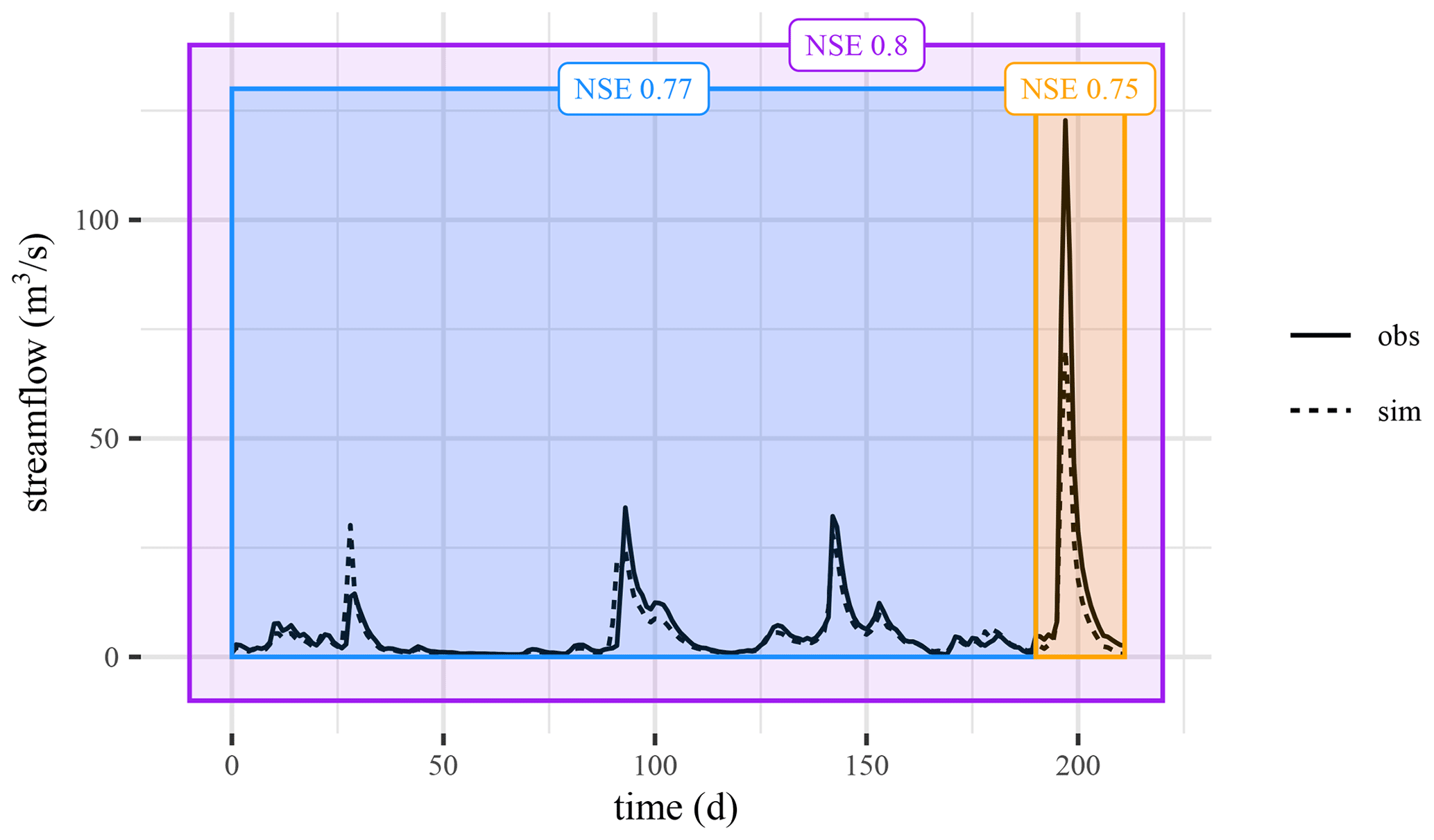
Figure 1Example of the part–whole relationship within the divide and measure nonconformity. The blue data partition has an NSE of 0.77, and the orange data partition (that contains the peak event) has an NSE of 0.75. However, the overall NSE is 0.8 (violet partition), which is larger than both individual partitions.
We refer to the phenomenon that the overall NSE can be higher than the NSEs of data subdivisions as the divide and measure nonconformity (DAMN). A natural question that follows from here is the following: what is the cause for the “DAMN behavior” in the example? To give an answer it is useful to consider the formal definition of the NSE:
where o represents observations, s represents simulations, t is an index variable (usually assumed as time), T is the overall number of time steps the NSE is computed over, and is the average of the observations.
This is the standard definition of the NSE and it contains several different interpretations for the source of the DAMN behavior. One interpretation is that the new event shifted the mean of the observational data (which the NSE uses as a reference model for comparisons; Schaefli and Gupta, 2007) so that the observational mean became a worse estimate for the first partition (blue) as a portion of the superset (purple). Another way to explain this behavior is that the NSE gives very different results for partitions with different variability. The variance of the observations in the second (orange) partition is higher than the variance of observations over the superset (purple), meaning that the denominator in the NSE calculation is higher if the numerator does not change. One can imagine taking the squared error term (the numerator of the NSE metric) over only the second (orange) partition but using the observational variance (the denominator of the NSE metric) from the whole (purple) time period. This would result in a value higher than the actual NSE value in the second period (orange).
The reflection from the previous paragraph concludes our motivational introduction. In what follows we provide a more in-depth exploration of the DAMN. We structure our exposition as follows: the remainder of the Introduction discusses related work (Sect. 1.1). Afterwards, we present our case study. Therein, we show that the overall NSE can only be equal to or higher than the NSE values of all possible partitions (Sects. 2 and Sect. 3; Sect. S2 provides a corresponding theoretical treatment showing that this behavior logically follows from the definition of the NSE). In the last part we present a short discussion of the implications of our work (Sect. 4) and our conclusions along with some recommendations for modelers (Sect. 5).
1.1 Related work
The NSE is so important to hydrological modeling that many publications exist that (critically) analyze its properties (e.g., Schaefli and Gupta, 2007; Mizukami et al., 2019; Clark et al., 2021; Gauch et al., 2023). Covering the full extent of the scientific discussion is out of scope for our Technical Note. Instead, we will mention the few publications that are most relevant: Gupta et al. (2009) use a decomposition of the NSE to show that the criterion favors models that provide conservative estimates of extremes. In contrast, our analysis provides a data-based view of how the NSE behaves when data are divided or combined. There is also a line of work that focuses on the statistical problems that arise with estimating model performance in small and limited data settings that we often encounter in hydrology (e.g., Lamontagne et al., 2020; Clark et al., 2021). For example, Clark et al. (2021) demonstrate inherent uncertainties of estimating the NSE and suggest using distributions of performance metrics to understand the inherent uncertainties. While their analysis focuses on the difficulties of finding a hypothetical “true NSE value”, we focus on a specific behavior that concerns the part–whole relationship of the criterion. We thus view this research avenue as perpendicular to ours. Lastly, we point to the studies of Schaefli and Gupta (2007), Seibert (2001), and more recently Duc and Sawada (2023), which argue that the NSE is not necessarily well-suited to compare rivers that exhibit different streamflow variances. Indeed, one can view the evaluation of multiple rivers as a form of assessing multiple partitions (the same logic as in our introductory example from Sect. 1 applies: whether the mean of a time series is a better or worse estimator depends mainly on the variance of the observations).
1.1.1 Statistical paradoxes
Statisticians have coined many paradoxes. In particular, the DAMN is closely related to Simpson's paradox (Simpson, 1951; Wagner, 1982). Simpson's paradox illustrates how positive statistical associations can be inverted under (non-random) data partitioning (Fig. 2). The DAMN can be seen as a special case of Simpson's paradox, since it describes the behavior of model performance metrics when (non-random) partitions of the data are combined (or, vice versa, when the data are divided into partitions). Similarly, an amalgamation paradox (sensu Good and Mittal, 1987) can be seen as a more general form of Simpson's paradox. It describes how statistical associations increase or decrease under different data combinations. Hence, the DAMN can also be seen as a special case of an amalgamation paradox, where the measured performance can always only increase when we combine data, compared to the lowest score found in the data subsets.
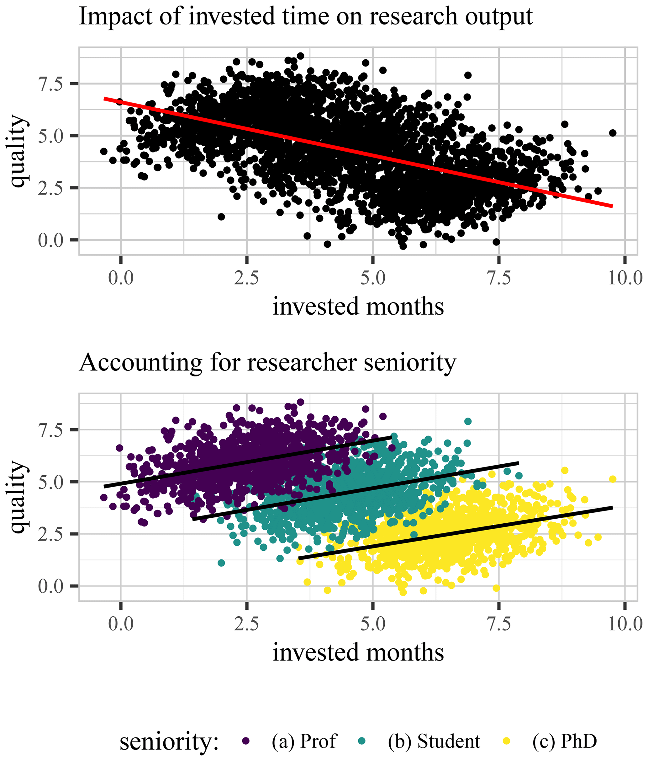
Figure 2Toy example illustrating Simpson's paradox, showing the relationship between the time spent studying and grades. Top panel: the “global” evaluation of the data suggests a negative effect of preparation time on the grade. Bottom panel: the “local” evaluation from splitting students by exam class shows a positive correlation between study time and grades. Evaluators should account for both patterns – the global and the local – depending on the purpose of the analysis. Adapted from Wayland (2018).
1.1.2 Limited sample size
For model evaluation more data typically help. This also holds true for situations where the DAMN is a concern, since the NSEs will behave less erratically when more data are used (see Clark et al., 2021). However, the DAMN as such is not a small-sample problem. It will occur whenever we divide the data into situations that have specific properties (e.g., when we divide the data along the temperature while having a model that has a high predictive performance for low temperature and low predictive performance for high temperatures). For example, the NSE remains susceptible to the DAMN independently of how well we are able to estimate the mean (or variance) of the data. That said, for the special case of time splits (for a given basin) it is indeed possible to argue that the occurrence of the DAMN is only due to limited data: if we had unlimited data for each partition, the inherent correlation structure (e.g., Shen et al., 2022) and the extreme value distribution of the streamflow (e.g., Clark et al., 2021) would not matter and our estimations of the mean (or variance) would converge to the same value for each partition – assuming no distribution shifts over time. Yet, sometimes we are interested in the performance of a model on subsets of the full available period, and for these cases no amount of overall available data will save us from the DAMN.
1.1.3 Models with uncertainty predictions
With access to models that provide not only point predictions but also richer forms of prediction (say, interval or distributional predictions), modelers get access to more model performance criteria. Many of these criteria are evaluated first on a per-sample level (e.g., by comparing the distributional estimation with the observed values) and then aggregated in a simple additive way (e.g., by taking the sum or the mean). Metrics based on proper scoring rules – such as the Winkler score (Winkler, 1972) for interval or the log-likelihood for distributional predictions – or metrics derived from information theoretical consideration (such as the cross-entropy) generally follow this scheme and are therefore typically not susceptible to the DAMN (see Sect. S2).
We conduct two distinct experiments. The first experiment is purely a synthetic study. It examines how the overall NSE relates to different NSE values of the partitions. The goal is to empirically show that the overall NSE can be higher (but not lower) than all of the individual NSE values of a partition. In the second experiment, we make a comparative analysis of the NSE and a derived “DAMN-safe” performance criterion. This experiment is based on real-world data. Our goal is to examine the implications of the DAMN for a particular example. In the following subsections we explain both experimental parts in more detail.
2.1 Synthetic study
Our synthetic experiment demonstrates that the overall performance of a model (as measured by the NSE) is in many cases higher than what all situational or data split performances would suggest. The setup is loosely inspired by Matejka and Fitzmaurice (2017): all data for the experiment derive from a single gauging station (namely, Priest Brook Near Winchendon –USGS ID no. 01162500 – from Addor et al., 2017).
To generate simulations we (1) copied the streamflow observation data, (2) added noise to those observation data, (3) clipped any resulting negative values to zero (to avoid streamflow that is trivially implausible), and (4) further optimized the resulting streamflow values themselves to reach a certain prescribed NSE by using gradient descent. That is, we modify the data points of the simulation (which in itself is just the observation with some noise) along the gradient given our loss function – and until the warranted performance (say, an NSE of 0.7) is reached. This allows us to build simulations that have defined NSE values for the data partitions. Specifically, we partition the observed streamflow into two parts: (1) “low flows” that fall below a threshold and (2) “high flows” that are at or above said threshold. We set the threshold using a desired fraction of data being designated as low or high flows. For example, w=0.2 means the 20 % smallest streamflow values are contained in the low-flow partition. We will refer to the NSE of the low flows as NSElow and the NSE of the high flows as NSEhigh. We fix low-flow performance to NSElow=0.5 using the procedure outlined above (for runs with other fixed parameters Sect. S3 provides similar results for NSElow=0.25 and NSElow=0.75). From a technical standpoint it is arbitrary for our experiment which of the two partitions has a fixed performance. However, we chose the low-flow partition since it is perhaps easier to think about what would happen if we have more or fewer high-flow data. We vary both w and NSEhigh between 0.1 and 0.9. For each point of the resulting grid we have three NSE values: (1) NSElow, (2) NSEhigh, and (3) the overall NSEall. We measure the practical effect of the DAMN using the signed distance of NSEall to the nearest edge of the NSEs of the partitions (either NSElow or NSEhigh):
where and as shown in Fig. 3.
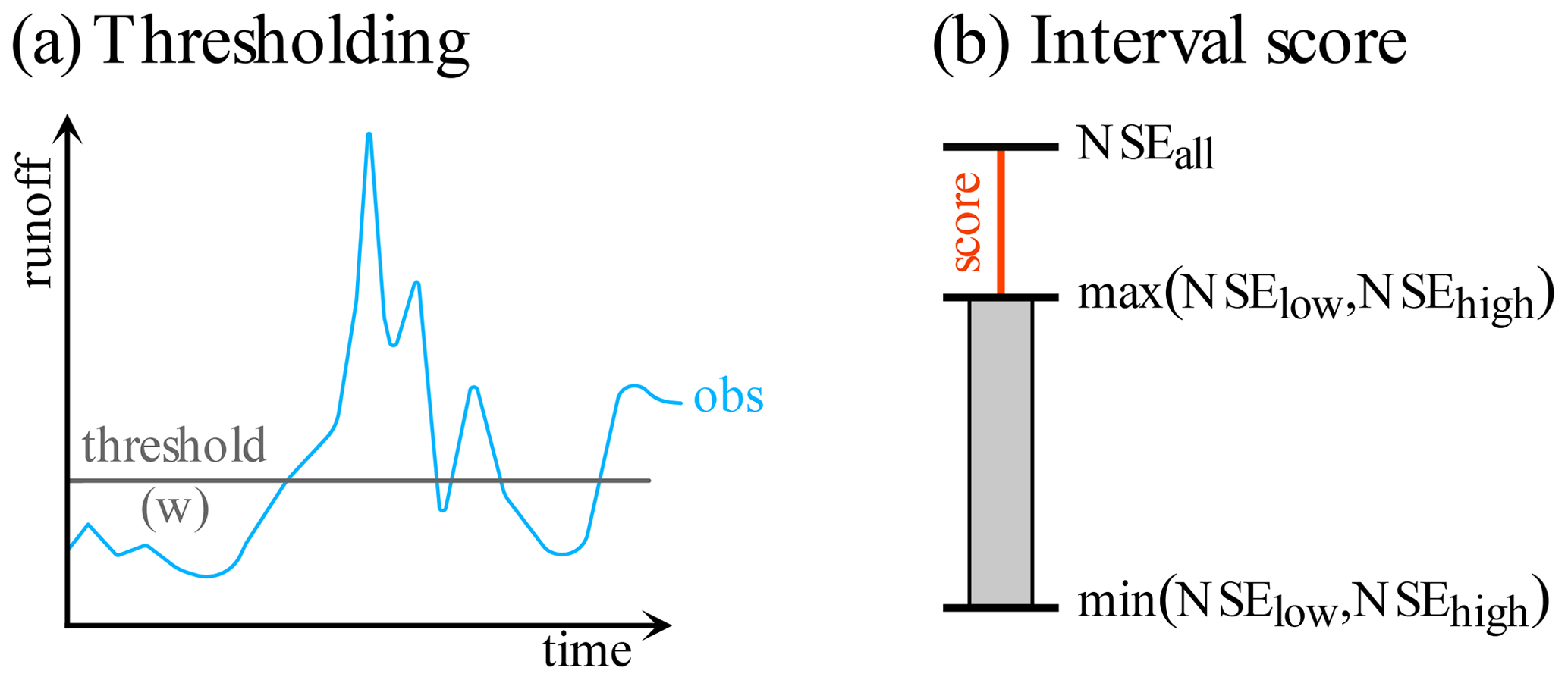
Figure 3Exemplary depiction of the experimental setup. (a) For each model evaluation the data are split into two parts by a runoff threshold and three NSEs are computed: NSElow for data below the threshold, NSEhigh for data above the threshold, and NSEall for all data. (b) Then, the interval score is computed as the signed distance of NSEall from the interval between the NSElow and the NSEhigh.
2.2 Comparative analysis
Our comparative analysis shows the influence of the DAMN by juxtaposing the behavior of the NSE with a derived performance criterion. This criterion is probably the simplest modification of the NSE that renders it DAMN-safe. However, our intention with the new criterion is not to propose a new metric for hydrologists (even if it could be used as such). Rather, we want to introduce the criterion as a tool for thought to reason about the DAMN.
The most straightforward NSE modification we found is to use a fixed reference partition for the denominator of the NSE. That is, instead of re-estimating the observational mean within the NSE for each (new) partition, we first choose a reference split and then compute the estimated variance from it (we also explored other more complex modifications but found them to be less insightful; Sect. S1 in the Supplement provides an example of such an exploration). Given the simple nature of the modification, we refer to the “new” performance criterion as low-effort NSE (LENSE):
where t is the sample index (which can but does not necessarily have to be a time index), is the mean of the observations from a to-be-chosen reference partition, T represents the total number of time steps in the evaluated partition, and TR represents the number of time steps in the reference partition. In a certain sense, both T and TR are a result of the modification, since the different partitions for computing the errors and the observational variance make it so that the fractions are not necessarily reduced.
The LENSE follows a straightforward design principle: we use a reference set that is independent of the partition to transform the right-hand side of NSE into a special case of a weighted mean squared error. This principle makes the LENSE DAMN-safe because the denominator re-normalizes the squared error for each partition using the same constant (Sect. S2.3 and S2.4 provide the corresponding formal proofs for the weighted mean squared error and the LENSE, respectively). In practice, the only advantage of the LENSE over using the MSE for expressing the model performance would be that the LENSE provides a similar range of interpretation as the NSE.
The choice of the reference partition largely determines its interpretation. If, for example, the mean is supposed to be an estimate of the (true) mean of an underlying distribution (like, for example, in Schaefli and Gupta, 2007), then we should use as many data as possible to estimate it. In this case, it would be logical to use all data for the estimation – i.e., training (in hydrology we refer to this partition as the calibration set), validation (in hydrology this partition typically does not exist or is subsumed into the calibration set), and test (in hydrology we refer to this partition as the validation set). If, on the other hand, we interpret the mean as a baseline model (like, for example, in Knoben et al., 2019), then it makes sense to also use just the data that were used for model selection for the estimation of the mean. One could also use the test split as a reference and recreate the NSE (the crucial difference is that it is not allowed to update the reference split if new data arrive). Since the most convenient choice for such a reference split is the training (calibration) split, we propose using it for the canonical application of LENSE (also, this split remains unchanged when new data arrive for the model to be used in the future).
The LENSE is robust against the DAMN by design. Thus, measuring its interval score with our synthetic setup will yield zero values everywhere. We did indeed try this as a check but do not show these results explicitly since very little information is provided (we nevertheless encourage interested readers to explore this by using the code we provide). However, it is still insightful to compare how the LENSE and the NSE behave. Specifically, we explore two aspects. To that end we use the model and real-world data from Kratzert et al. (2019). First, we show how the performance criteria compare when we evaluate them for the 531 basins from Kratzert et al. (2019). Here, we evaluate NSE as in Kratzert et al. (2019) and use the training period as the reference partition for LENSE. Second, we inspect the overall performance according to the NSE and LENSE related to the corresponding performances of different hydrological years for an arid catchment. We specifically chose an arid catchment here, since the mean of the runoff varies there more considerably between individual hydrological years. As before, we use the training period as the reference partition for the LENSE.
For both parts of the comparative analysis we use the ensemble Long Short-Term Memory (LSTM) network from Kratzert et al. (2019) as hydrological models, but note that the model choice is not of importance (for comparison, Sect. S3.1 provides some example cumulative distribution functions for other models).
3.1 Synthetic study
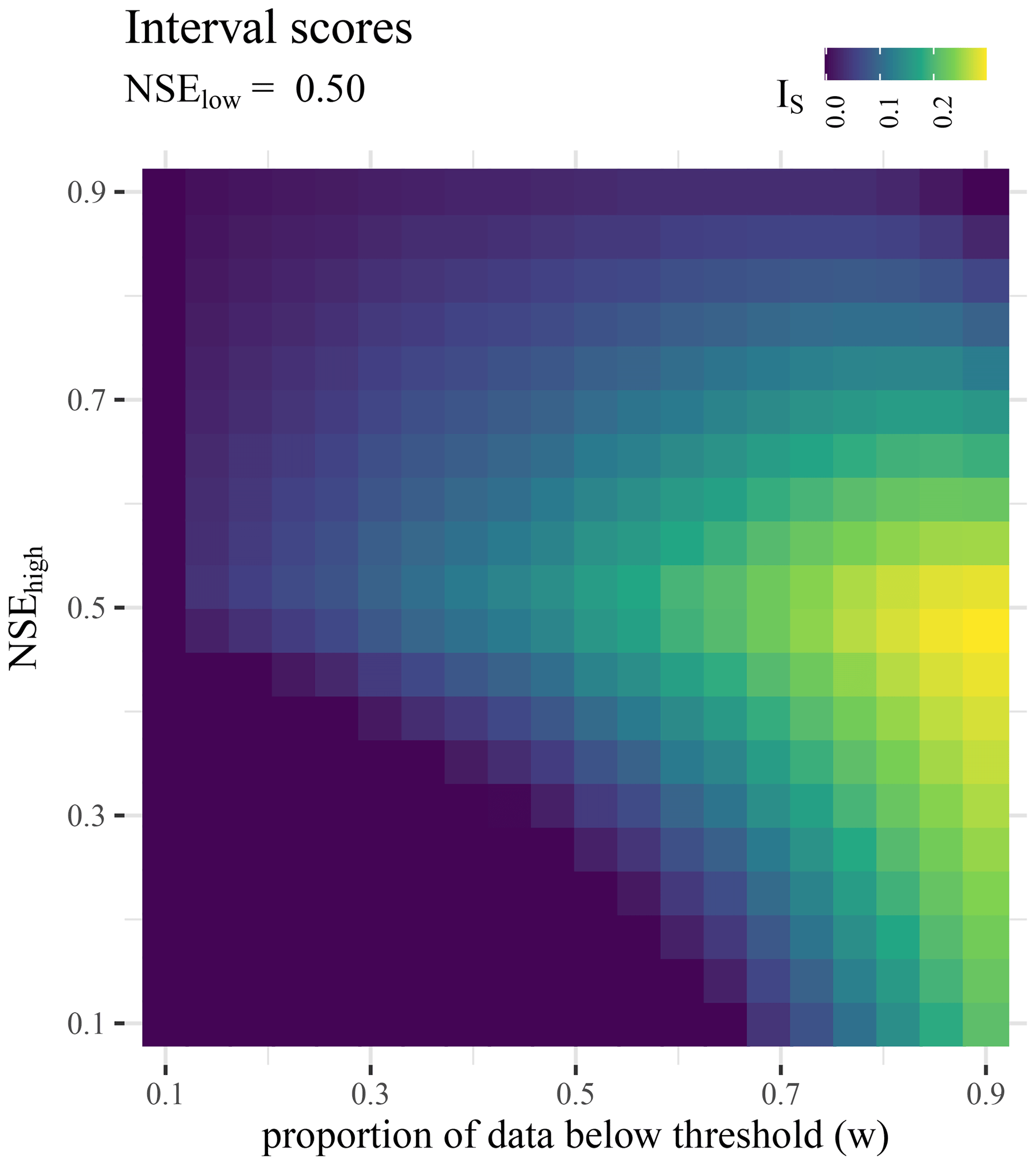
Based on our synthetic experiment we find that NSEall can be outside of the range of the NSEs spanned by the partitions (Fig. 4). Furthermore, the absence of negative interval scores indicates that the lowest-valued NSE of all partitions is a lower bound for NSEall, which we confirm with theoretical considerations (Sect. S2). Similarly, the existence of positive interval scores indicates that there is no trivial upper bound for the NSEall below its maximum of 1. We can also see that the interval scores tend to be highest when the NSEs of the partitions are equal – that is, . Intuitively from a statistical perspective, this makes sense: this is where the interval is the thinnest – and due to the lower bound, the NSEall can only be above or exactly equal. Interestingly though, the highest interval score is only reached with the largest lower partition we considered (90 % of the data). Here, we not only have the thin interval, but this is also the situation where we would expect the mean of the high-flow data to be the furthest from the mean of the low flows (since the mean of the low flows does not change much with the additional high flows, while the highest high flows have a substantially higher mean than the lower ones). Thus, when we introduce the high-flow data into the NSEall computation it yields the largest difference.
Further, if we look at the overall pattern of interval scores in Fig. 4, we can see that even if the overall performance is relatively good (say, an NSEhigh of 0.7) the interval scores (and hence the distances to a situational NSE value) can become quite large. As a matter of fact, in terms of situational performances the interval score is only some sort of best-case scenario, since it only measures the distance to the better of the score of the partitions.
3.2 Comparative analysis: NSE and LENSE
The comparison of the NSE and the LENSE for the LSTM ensemble and the 531 basins from Kratzert et al. (2019) shows that the LENSE tends to yield lower values than the NSE, except for the best-performing basins (Fig. 5). There, the LENSE values are slightly higher than the NSE values. However, since the performance on these basins is already very close to the theoretical best value (which is 1 for both criteria) the differences there are tiny.
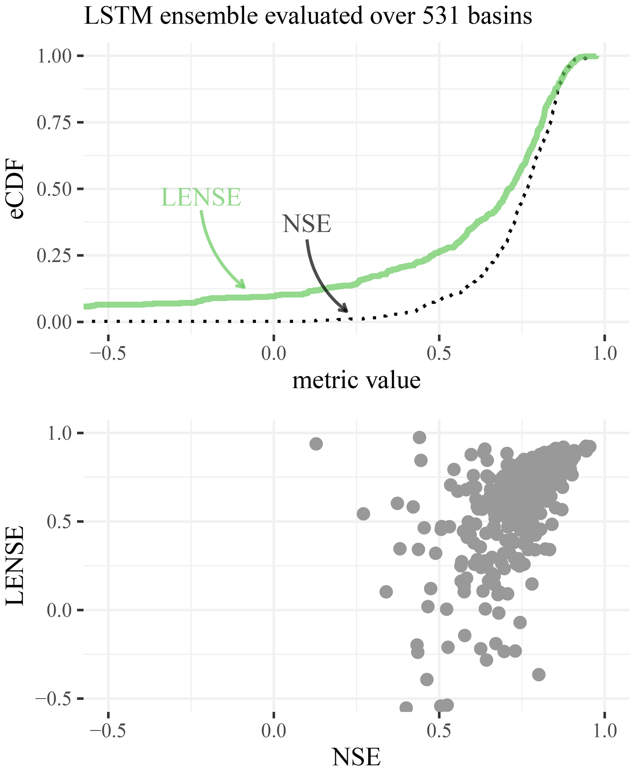
Figure 5The plot above shows the empirical cumulative distribution functions of the NSE (dotted black line) and the LENSE (green line) for the 531 basins used in Kratzert et al. (2019) and the corresponding LSTM ensemble runs. The scatter plot below shows the non-cumulative relation between the NSE and the LENSE.
For the yearly evaluation on an individual basin the NSE can vary substantially (Fig. 6). We note first that the LENSE exhibits fewer variations over the years than the NSE. Further, we can see that the overall LENSE is nicely enclosed within the values from the individual years – while the overall NSE is not. For 4 years the NSE values fall below 0.0, and for 2 of the 4 they are below −0.5. These values are of particular interest because the overall NSE is above 0.7. A naive interpretation would suggest that the model degrades in performance in these years. However, a comparison to the respective LENSE values indicates that what we see here is largely an effect of the DAMN.
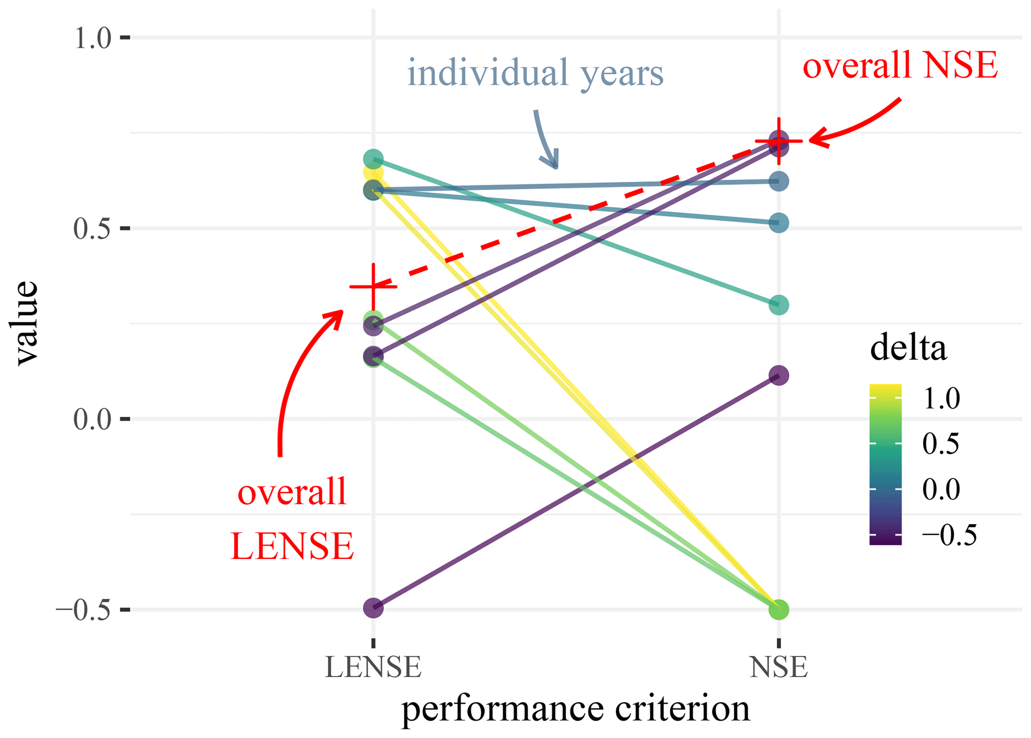
Figure 6Comparison of NSE and LENSE in an arid basin. The colored dots show the performance for different hydrological years in the validation period (the color indicates the magnitude of the performance difference); the crosses show the respective performances for the entire validation period. We truncated the values to −0.5 to show the pattern more clearly. The relatively large downward variability of NSE values exists because for some years the mean becomes an extremely good estimate for the daily runoff within certain periods. The LENSE, on the other hand, does not recompute the mean in the denominator for each validation year and has a stable estimation of the observational variance; see Eq. (3). It is therefore more stable and less susceptible to such outlier years.
Another interesting phenomenon is that the NSE values from 3 hydrological years are higher than the corresponding LENSE values. The worst LENSE values (−0.5) correspond to an NSE that is above 0.0, which is far away from the supposed worst performance in terms of the NSE. This suggests that the year had a relatively high streamflow variance, with a relatively bad simulation.
To conclude, we re-emphasize that the purpose of the LENSE is not to propose a new metric or to replace the NSE. The performance values from LENSE should not be considered “more true” than those of the NSE. Rather, they show different aspects of the model behavior that are in the data but are easily overlooked if one only focuses on the NSE alone.
Some specific examples where modelers should consider DAMN-like phenomena are as follows.
-
Approaches that rely on sliding windows (e.g., Wagener et al., 2003). Here, one cannot derive the overall performance from the performances over different windows of the data, and NSE values calculated over sliding windows might appear smaller than the ones calculated over longer time periods of the same data.
-
Aggregating or comparing separate evaluation of different rivers – for example, as was done by Kratzert et al. (2019). For basins with low runoff variability, the mean is a better estimator than for basins with high variability. Our analysis suggest that in this case the relative performance does not necessarily suggest model failure, but could also be related to the DAMN, since the mean is a very strong baseline for the arid catchment (which induces erratic NSE behavior).
-
Differential split settings that divide the hydrograph into low flows and high flows (e.g., Klemeš, 1986). In this case, the low-flow NSE can be prone to having low values because the mean is a good estimator. Yet, high-flow NSEs will often suffer from larger overall errors.
These examples represent settings where the DAMN appears very prominently. However, our findings generalize to any study that draws conclusions about model performance while using “DAMN-susceptible” metrics over different periods. For example, the Kling–Gupta efficiency (KGE; Gupta et al., 2009) exhibits similar empirical behavior to the NSE (we do not show this explicitly in this note but encourage readers to explore it, e.g., by using our code, which provides an implementation of the KGE for testing). That said, simple average-based metrics such as MSE are not subject to the DAMN (see Sect S2.2).
Random partitions and data splitting
Data splitting is common practice in machine learning and data analysis. To our knowledge, the oldest records of data splitting go back in the early 20th century (Larson, 1931; Highleyman, 1962; Stone, 1974; Vapnik, 1991). These classical cases and the approaches that derived from them use random splitting. Although the DAMN can also occur with random subsets of the data (our theory applies also there; Sect. S2) it is less of a concern there, since for independent sampling the overall NSE value should not deviate too much from the NSE values of the partitions. The intuition here follows the one given in our exemplary introduction (Sect. 1): according to expectation, the means of two random partitions provide the same reference models. In hydrology, two common situational (i.e., non-random) data splits exist: (1) the spatial data split between catchments (e.g., Kratzert et al., 2019; Mai et al., 2022) and (2) the temporal data split for validating (for a recent discussion see Shen et al., 2022). Regarding (1), Feng et al. (2023) recently proposed an ad hoc regional data partitioning for model evaluation. A perhaps more principled form of this technique can be found in the data-based splitting that has been put forward independently by Mayr et al. (2018) and Sweet et al. (2023). On their own terms, both propose partitioning the data based on feature clusters. Either way, this type of informed (non-random) splitting is susceptible to the DAMN. Regarding (2), Klemeš (1986) introduced a style of twofold (cross-)validation to hydrology. Inter alia, he proposed the so-called differential split sample test. It is a type of non-random split that subdivides a hydrograph into parts that reflect specific hydrological processes – say, low-flow and high-flow periods. This type of splitting is common in hydrology, but since it is also an informed (non-random) splitting it is indeed exposed to the DAMN. Here, we do not want to say that the community should refrain from differential split sampling. On the contrary, we believe that it should remain a part of the hydrological model building toolbox. However, when using it modelers should be aware of the DAMN and how it limits potential conclusions for model comparisons.
Likewise, we do not argue against using the NSE for model comparisons. Even if there are limits to what the metric can express, we assert that NSE remains a well-established assessment tool with many desired properties (in this context we would also like to refer readers to Schaefli and Gupta, 2007, for a more specific discussion of the limits of the NSE for comparing model performance across different basins). Hence, our goal is to shine light on the specific behavior of metrics that are not DAMN-safe (the NSE being the most prominent example thereof). That is, the DAMN can make comparisons more difficult when data are split into partitions with widely different statistical properties (say, rivers or periods with very low variance and rivers or periods with very high variance in streamflow).
This contribution examines a part–whole relation that we term “divide and measure nonconformity” (DAMN). Specifically, the DAMN describes the phenomenon that the NSE of all the data can be higher than all the NSEs of subsets that together comprise the full dataset. That is, the global NSE can show counterintuitive behavior by not being bounded by the NSE values in all its subsets. From a statistical point of view, the DAMN can therefore be seen as a sort of amalgamation paradox (Good and Mittal, 1987), and despite its counterintuitive appearance, the behavior can be well-explained. Our goal with this Technical Note is not to eliminate the DAMN but rather to make modelers more aware of it, explain how it manifests itself, and provide tools to check and think about it. If we study model behavior in specific situations, we need to be aware of the DAMN.
Although our treatment revolves almost exclusively around NSE, many performance criteria are “DAMN-susceptible”. As demonstrated by our introduction of LENSE (a pseudo-performance criterion that serves as a thinking tool in our discussion), the strength of the effect depends mainly on the design of a given criterion. If a performance criterion is prone to the DAMN it implies that we cannot infer the global performance from looking at local performances.
With regard to follow-up work, we believe that our experimental setup suggests an interesting avenue for inquiry, which we shall call “NSE kinetics” – that is, to study how easy it is to improve or worsen the NSE by changing the observations or simulations with a given budget or constraints. For example, it might be easy to improve (worsen) the performance for basins where a model is weak by randomly improving some time points (by just adding noise). However, if one wants to improve (worsen) the simulation for a basin with pronounced seasonality and large amounts of high-quality data it might require a larger budget and changes to specific events. Studies like that might have potential to render the behavior of the NSE clearer. They might even allow the community to derive (quantitative) comparisons for the “flexibility/response” of different metrics. Scientists have studied the sensitivity and uncertainty of the NSE (e.g., Wright et al., 2015; Clark et al., 2021, respectively). Yet, as far as we know, no one has yet examined a principled approach that is able to quantify the ease of change with respect to a given direction.
We conclude with the observation that the existence of phenomena like the DAMN underlines the importance of evaluating models with a range of different metrics – preferably tailored to the specific application at hand (Gauch et al., 2023). On top of that, we would like to push the community (and ourselves) to also always evaluate models with regard to the predictive uncertainty when doing model comparisons and benchmarking exercises (e.g., Nearing et al., 2016, 2018; Mai et al., 2022; Beven, 2023). Typically, this will result in an additional workload for modelers, since it often means that a method for providing uncertainty estimates needs to be built (on top of a hydrological model that gives point predictions). However, existing uncertainty performance criteria (e.g., the log-likelihood, the Winkler score, or the continuous ranked probability score) not only provide additional information, but are also largely robust against the DAMN (this is because they are usually computed for each data point and then aggregated by taking a sum or an average). Further, uncertainty plays an important role for hydrological predictions and should thus be included in our benchmarking efforts.
We will make the code and data for the experiments and data from all produced results available online. The code for the experiments can be found at https://github.com/danklotz/a-damn-paper/tree/main (Klotz, 2024). The hydrological simulations are based on the data from Kratzert et al. (2019) and on the open-source Python package NeuralHydrology (Kratzert et al., 2022). The streamflow that we used is from the publicly available CAMELS dataset by Newman et al. (2015) and Addor et al. (2017).
The supplement related to this article is available online at: https://doi.org/10.5194/hess-28-3665-2024-supplement.
DK had the initial idea for the paper. DK and MG set up the experiment (and also many negative results along the way). MG came up with the first version of the SENSE criterion. DK and MG realized the theoretical Supplement material and JZ checked it. DK, GN, and JZ conceptualized the paper structure. All authors contributed to the analysis of the results, the discussion of the interpretations, and the creation of the figures, as well as the writing process.
The contact author has declared that none of the authors has any competing interests.
Publisher's note: Copernicus Publications remains neutral with regard to jurisdictional claims made in the text, published maps, institutional affiliations, or any other geographical representation in this paper. While Copernicus Publications makes every effort to include appropriate place names, the final responsibility lies with the authors.
We are grateful for the support and guidance of Sepp Hochreiter, who is always generous with his time and ideas. We would also like to thank Lukas Gruber for insightful discussions regarding our theoretical considerations of DAMN. Due to his critical eye the Supplement became much more thorough. Further, we need to mention Claus Hofman, Andreas Radler, and Annine Duclaire Kenne for bouncing off ideas for the experiments, even if they ultimately did not materialize as we imagined.
The article processing charges for this open-access publication were covered by the Helmholtz Centre for Environmental Research – UFZ.
This paper was edited by Nadav Peleg and reviewed by Hoshin Gupta, Wouter Knoben, and one anonymous referee.
Addor, N., Newman, A. J., Mizukami, N., and Clark, M. P.: The CAMELS data set: catchment attributes and meteorology for large-sample studies, Hydrol. Earth Syst. Sci., 21, 5293–5313, https://doi.org/10.5194/hess-21-5293-2017, 2017. a, b
Beven, K.: Benchmarking hydrological models for an uncertain future, Hydrol. Process., 37, e14882, https://doi.org/10.1002/hyp.14882, 2023. a
Clark, M. P., Vogel, R. M., Lamontagne, J. R., Mizukami, N., Knoben, W. J., Tang, G., Gharari, S., Freer, J. E., Whitfield, P. H., Shook, K. R., and Papalexiou, S. M.: The abuse of popular performance metrics in hydrologic modeling, Water Resour. Res., 57, e2020WR029001, https://doi.org/10.1029/2020WR029001, 2021. a, b, c, d, e, f
Duc, L. and Sawada, Y.: A signal-processing-based interpretation of the Nash–Sutcliffe efficiency, Hydrol. Earth Syst. Sci., 27, 1827–1839, https://doi.org/10.5194/hess-27-1827-2023, 2023. a
Feng, D., Beck, H., Lawson, K., and Shen, C.: The suitability of differentiable, physics-informed machine learning hydrologic models for ungauged regions and climate change impact assessment, Hydrol. Earth Syst. Sci., 27, 2357–2373, https://doi.org/10.5194/hess-27-2357-2023, 2023. a
Gauch, M., Kratzert, F., Gilon, O., Gupta, H., Mai, J., Nearing, G., Tolson, B., Hochreiter, S., and Klotz, D.: In Defense of Metrics: Metrics Sufficiently Encode Typical Human Preferences Regarding Hydrological Model Performance, Water Resour. Res., 59, e2022WR033918, https://doi.org/10.1029/2022WR033918, 2023. a, b
Good, I. J. and Mittal, Y.: The amalgamation and geometry of two-by-two contingency tables, Ann. Stat., 15, 694–711, https://doi.org/10.1214/aos/1176350369, 1987. a, b
Gupta, H. V., Kling, H., Yilmaz, K. K., and Martinez, G. F.: Decomposition of the mean squared error and NSE performance criteria: Implications for improving hydrological modelling, J. Hydrol., 377, 80–91, 2009. a, b
Highleyman, W. H.: The design and analysis of pattern recognition experiments, Bell Syst. Tech. J., 41, 723–744, 1962. a
Klemeš, V.: Operational testing of hydrological simulation models, Hydrolog. Sci. J., 31, 13–24, 1986. a, b
Klotz, D.: Acompaning code for Technical Note: The divide and measure nonconformity, GitHub [code], https://github.com/danklotz/a-damn-paper/tree/main, last access: 7 August 2024. a
Knoben, W. J. M., Freer, J. E., and Woods, R. A.: Technical note: Inherent benchmark or not? Comparing Nash–Sutcliffe and Kling–Gupta efficiency scores, Hydrol. Earth Syst. Sci., 23, 4323–4331, https://doi.org/10.5194/hess-23-4323-2019, 2019. a
Kratzert, F., Klotz, D., Shalev, G., Klambauer, G., Hochreiter, S., and Nearing, G.: Towards learning universal, regional, and local hydrological behaviors via machine learning applied to large-sample datasets, Hydrol. Earth Syst. Sci., 23, 5089–5110, https://doi.org/10.5194/hess-23-5089-2019, 2019. a, b, c, d, e, f, g, h, i
Kratzert, F., Gauch, M., Nearing, G., and Klotz, D.: NeuralHydrology – A Python library for Deep Learning research in hydrology, J. Open Sour. Softw., 7, 4050, https://doi.org/10.21105/joss.04050, 2022. a
Lamontagne, J. R., Barber, C. A., and Vogel, R. M.: Improved Estimators of Model Performance Efficiency for Skewed Hydrologic Data, Water Resourc. Res., 56, e2020WR027101, https://doi.org/10.1029/2020WR027101, 2020. a
Larson, S. C.: The shrinkage of the coefficient of multiple correlation, J. Educ. Psychol., 22, 45–55, https://doi.org/10.1037/h0072400, 1931. a
Mai, J., Shen, H., Tolson, B. A., Gaborit, É., Arsenault, R., Craig, J. R., Fortin, V., Fry, L. M., Gauch, M., Klotz, D., Kratzert, F., O'Brien, N., Princz, D. G., Rasiya Koya, S., Roy, T., Seglenieks, F., Shrestha, N. K., Temgoua, A. G. T., Vionnet, V., and Waddell, J. W.: The Great Lakes Runoff Intercomparison Project Phase 4: the Great Lakes (GRIP-GL), Hydrol. Earth Syst. Sci., 26, 3537–3572, https://doi.org/10.5194/hess-26-3537-2022, 2022. a, b
Matejka, J. and Fitzmaurice, G.: Same stats, different graphs: generating datasets with varied appearance and identical statistics through simulated annealing, in: Proceedings of the 2017 CHI conference on human factors in computing systems, Denver, Colorado, USA, 6–11 May 2017, 1290–1294, https://doi.org/10.1145/3025453.3025912, 2017. a
Mayr, A., Klambauer, G., Unterthiner, T., Steijaert, M., Wegner, J. K., Ceulemans, H., Clevert, D.-A., and Hochreiter, S.: Large-scale comparison of machine learning methods for drug target prediction on ChEMBL, Chem. Sci., 9, 5441–5451, 2018. a
Mizukami, N., Rakovec, O., Newman, A. J., Clark, M. P., Wood, A. W., Gupta, H. V., and Kumar, R.: On the choice of calibration metrics for “high-flow” estimation using hydrologic models, Hydrol. Earth Syst. Sci., 23, 2601–2614, https://doi.org/10.5194/hess-23-2601-2019, 2019. a
Nash, J. E. and Sutcliffe, J. V.: River flow forecasting through conceptual models part I – A discussion of principles, J. Hydrol., 10, 282–290, 1970. a
Nearing, G. S., Mocko, D. M., Peters-Lidard, C. D., Kumar, S. V., and Xia, Y.: Benchmarking NLDAS-2 soil moisture and evapotranspiration to separate uncertainty contributions, J. Hydrometeorol., 17, 745–759, 2016. a
Nearing, G. S., Ruddell, B. L., Clark, M. P., Nijssen, B., and Peters-Lidard, C.: Benchmarking and process diagnostics of land models, J. Hydrometeorol., 19, 1835–1852, 2018. a
Newman, A. J., Clark, M. P., Sampson, K., Wood, A., Hay, L. E., Bock, A., Viger, R. J., Blodgett, D., Brekke, L., Arnold, J. R., Hopson, T., and Duan, Q.: Development of a large-sample watershed-scale hydrometeorological data set for the contiguous USA: data set characteristics and assessment of regional variability in hydrologic model performance, Hydrol. Earth Syst. Sci., 19, 209–223, https://doi.org/10.5194/hess-19-209-2015, 2015. a
Schaefli, B. and Gupta, H. V.: Do Nash values have value?, Hydrol. Process., 21, 2075–2080, 2007. a, b, c, d, e
Seibert, J.: On the need for benchmarks in hydrological modelling, Hydrol. Process., 15, 1063–1064, https://doi.org/10.1002/hyp.446, 2001. a
Shen, H., Tolson, B. A., and Mai, J.: Time to update the split-sample approach in hydrological model calibration, Water Resour. Res., 58, e2021WR031523, https://doi.org/10.1029/2021WR031523, 2022. a, b
Simpson, E. H.: The interpretation of interaction in contingency tables, J. Roy. Stat. Soc. B, 13, 238–241, 1951. a
Stone, M.: Cross-validatory choice and assessment of statistical predictions, J. Roy. Stat. Soc. B, 36, 111–133, 1974. a
Sweet, L.-b., Müller, C., Anand, M., and Zscheischler, J.: Cross-validation strategy impacts the performance and interpretation of machine learning models, Artific. Intel. Earth Syst., 2, e230026, https://doi.org/10.1175/AIES-D-23-0026.1, 2023. a
Vapnik, V.: Principles of risk minimization for learning theory, Adv. Neural Inform. Process. Syst., 4, 831–838, 1991. a
Wagener, T., McIntyre, N., Lees, M., Wheater, H., and Gupta, H.: Towards reduced uncertainty in conceptual rainfall-runoff modelling: Dynamic identifiability analysis, Hydrol. Process., 17, 455–476, 2003. a
Wagner, C. H.: Simpson's paradox in real life, Am. Stat., 36, 46–48, 1982. a
Wayland, J.: Jon Wayland: What is Simposon's Paradox, https://www.quora.com/What-is-Simpsons-paradox/answer/Jon-Wayland (last access: 13 December 2023), 2018. a
Winkler, R. L.: A decision-theoretic approach to interval estimation, J. Am. Stat. Assoc., 67, 187–191, 1972. a
Wright, D. P., Thyer, M., and Westra, S.: Influential point detection diagnostics in the context of hydrological model calibration, J. Hydrol., 527, 1161–1172, 2015. a