A decomposition approach to evaluating the local performance of global streamflow reanalysis

While global streamflow reanalysis has been evaluated at different spatial scales to facilitate practical applications, its local performance in the time–frequency domain is yet to be investigated. This paper presents a novel decomposition approach to evaluating streamflow reanalysis by combining wavelet transform with machine learning. Specifically, the time series of streamflow reanalysis and observation are respectively decomposed and then the approximation components of reanalysis are evaluated against those of observed streamflow. Furthermore, the accumulated local effects are derived to showcase the influences of catchment attributes on the performance of streamflow reanalysis at different scales. For streamflow reanalysis generated by the Global Flood Awareness System, a case study is devised based on streamflow observations from the Catchment Attributes and Meteorology for Large-sample Studies. The results highlight that the reanalysis tends to be more effective in characterizing seasonal, annual and multi-annual features than daily, weekly and monthly features. The Kling–Gupta efficiency (KGE) values of original time series and approximation components are primarily influenced by precipitation seasonality. High values of KGE tend to be observed in catchments where there is more precipitation in winter, which can be due to low evaporation that results in reasonable simulations of soil moisture and baseflow processes. The longitude, mean precipitation and mean slope also influence the local performance of approximation components. On the other hand, attributes on geology, soils and vegetation appear to play a relatively small part in the performance of approximation components. Overall, this paper provides useful information for practical applications of global streamflow reanalysis.

1 Introduction

Global streamflow reanalysis provides valuable information for water resources management (Beck et al., 2017; Harrigan et al., 2020; Pokhrel et al., 2021). Generated by using climate reanalysis to drive global hydrological models (GHMs; Alfieri et al., 2020; Hersbach et al., 2020; Muñoz-Sabater et al., 2021), there exist multiple streamflow reanalysis datasets, e.g., the Global Flood Awareness System (GloFAS) within the European Centre for Medium-Range Weather Forecasts (ECMWF)'s latest global atmospheric reanalysis (GloFAS-ERA5; Harrigan et al., 2020), the Global Reach-Level A Priori Discharge Estimates for SWOT (GRADES; Lin et al., 2019) and the Global Reach-Level Flood Reanalysis (GRFR; Yang et al., 2021). In practice, streamflow reanalysis can bridge the data gaps for ungauged and poorly gauged catchments and provides estimates on a large spatial scale and with sufficient temporal resolution (Lin et al., 2019; Harrigan et al., 2020; Yang et al., 2021). For example, the recent GloFAS-ERA5 provides streamflow information at the daily time step and with a spatial resolution of 0.1° across the globe (Harrigan et al., 2020).

The local performance plays a critical part in practical applications of global streamflow reanalysis (Veldkamp et al., 2018; Munia et al., 2020; Feng et al., 2021). By evaluating global reanalysis against observed streamflow, diagnostic plots and verification metrics are generated to showcase its local performance (Xie et al., 2019; Gao et al., 2020; Cantoni et al., 2022; Huang et al., 2022; Zhao et al., 2022a; Han et al., 2023; Liu et al., 2023). In the meantime, hydrological signatures derived from reanalysis are compared to those obtained from observed streamflow to facilitate insights into the effectiveness of hydrological models (Beck et al., 2017; Chen et al., 2022; Zhao et al., 2022b). For example, the performances of 10 Inter-Sectoral Impact Model Intercomparison Project (ISI-MIP) models are evaluated for low, mean and high flows using five streamflow percentile series (Chen et al., 2021). Considering limited observation data, streamflow reanalysis can serve as reference data to calibrate hydrological models, and then the model outputs can be compared to observations to see whether practical applications are available (Senent-Aparicio et al., 2021).

Time series analysis is one of the most important approaches to investigating the performance of hydrological models (Saraiva et al., 2021; Manikanta and Vema, 2022; Guo et al., 2022). From the perspective of time series, hydrological simulations are a combination of the components of periodic motion, trend, seasonality and error, which can be extracted by using decomposition approaches (Abebe et al., 2022; Manikanta and Vema, 2022; Xu et al., 2022). As one of the most important decomposition approaches, wavelet transform decomposes streamflow into time series of wavelet coefficients under certain frequencies (Manikanta and Vema, 2022). Therefore, it allows for multiresolution analysis compared to other decomposition approaches (Montoya et al., 2022). Owing to the time–frequency characterization, wavelet-based features of reanalysis and observed streamflow can be compared in order to zoom into detailed information for multiple time series segments (Manikanta and Vema, 2022). If there are errors in the reanalysis at specific timescales or during specific periods, the sources of these errors can be identified by the technique of time–frequency characterization (Lane, 2007).

While global streamflow reanalysis has been evaluated at different spatial scales (Harrigan et al., 2020; Chen et al., 2021; Senent-Aparicio et al., 2021), the time series characteristics of streamflow reanalysis in the time–frequency domain are yet to be investigated. Meanwhile, it is difficult to interpret the local performance of global streamflow reanalysis across different locations (Sichangi et al., 2016; Ghiggi et al., 2019; Tu et al., 2024), let alone the additional interpretation of the local performance at different timescales. This paper aims to bridge the gap by presenting a novel evaluation of global streamflow reanalysis by combining the discrete wavelet transform (DWT) with machine learning techniques. That is, the DWT is employed to exploit streamflow reanalysis in the time–frequency domain; then the accumulated local effects (ALEs) are derived by the random forest model to showcase the performance of original time series of reanalysis and its decomposed components at different scales. As will be demonstrated in the Methods and Results sections, streamflow reanalysis does exhibit different local performances at different timescales, and the influences of catchment attributes are illustrated.

2 Methods

2.1 Overview of the decomposition approach

A novel decomposition approach that combines the wavelet transform with machine learning techniques is proposed to evaluate global streamflow reanalysis in the time–frequency domain. There are three steps.

1. Decomposition of time series. The DWT is used to decompose the reanalysis and observed streamflow time series, resulting in “approximation” and “detail” components at different scales.

2. Verification of decomposed series. The Kling–Gupta efficiency (KGE), correlation, bias ratio and variability ratio are derived to indicate the local performance of original time series, approximation and detail components at various scales. In the meantime, the density-based spatial clustering of applications with noise (DBSCAN) algorithm is used to remove outliers from the verification metrics.

3. Influences of catchment attributes. The ALEs derived from the random forest model are employed to elaborate on the influences of catchment attributes and then identify the driving factors.

2.2 Decomposition of time series

Both reanalysis and observed streamflow time series are decomposed into approximation and detail components using the DWT (Chalise et al., 2023). It is executed by controlling the scaling and shifting factors associated with a mother wavelet (Nalley et al., 2012). Following Wei et al. (2012), the Daubechies wavelet of order 5 is used to decompose the streamflow time series (Talukder et al., 2020):

$$\begin{array}{}\text{(1)}& W(a,b)=\sum _{t\in Z}q\left(t\right){\mathit{\psi }}_{m,n}\left(t\right),\end{array}$$

in which q(t) is the time series to be decomposed, m and n are integers that respectively represent the amount of dilation and translation of the wavelet, t represents the discrete time, and ψ represents the wavelet basis function (Nalley et al., 2012):

$$\begin{array}{}\text{(2)}& {\mathit{\psi }}_{m,n}\left(t\right)={\mathrm{2}}^{-\frac{m}{\mathrm{2}}}\mathit{\psi }\left({\mathrm{2}}^{-m}t-n\right).\end{array}$$

The DWT decomposes a signal into approximation (low-frequency) and detail (high-frequency) coefficients, thereby separating its frequency components based on magnitude (Quilty and Adamowski, 2021). In the initial decomposition that utilizes high-pass and low-pass filters and inverse DWT, the original signal is decomposed into the detail component (D₁) and the approximation component (A₁). Subsequently, the approximation component (A₁) resulting from this initial stage is furthermore decomposed into D₂ and A₂, and so on for successive levels. This process is conducted from high-pass and low-pass filters followed by a down-sampling operator:

$$\begin{array}{}\text{(3)}& (q\downarrow \mathrm{2})\left[t\right]=q\left[\mathrm{2}t\right].\end{array}$$

Therefore, the streamflow time series is decomposed into the approximation coefficients and detail coefficients (Talukder et al., 2020):

$$\begin{array}{}\text{(4)}& \left\{\begin{array}{l}c{A}_l\left[t\right]=\sum _{n}L\left[n\right]q[\mathrm{2}t+n],\\ c{D}_l\left[t\right]=\sum _{n}H\left[n\right]q[\mathrm{2}t+n],\end{array}\right.\end{array}$$

in which cA_l[t] is the coefficient of approximation, cD_l[t] is the coefficient of detail, the subscript l represents the decomposition level, L is the low-pass filter and H is the high-pass filter. The inverse DWT is used to obtain the approximation components and detail components (Guo et al., 2022):

$$\begin{array}{}\text{(5)}& \left\{\begin{array}{l}{A}_l=\mathrm{IDWT}\left(c{A}_l\left[t\right]\right),\\ D_l=\mathrm{IDWT}\left(c{D}_l\left[t\right]\right),\end{array}\right.\end{array}$$

in which IDWT is the inverse DWT, A_l is approximation component and D_l is detail component in level l.

For reanalysis and observed streamflow time series, the decomposition is denoted as

$$\begin{array}{}\text{(6)}& \left\{\begin{array}{l}{d}_t=\sum _{l=\mathrm{1}}^{l_{\mathrm{m}}}{D}_{d,l}+A_{d,l_{\mathrm{m}}},\\ q_t=\sum _{l=\mathrm{1}}^{l_{\mathrm{m}}}{D}_{q,l}+A_{q,l_{\mathrm{m}}},\end{array}\right.\end{array}$$

in which d_t is the reanalysis, q_t is the observed streamflow and l_m is the maximum decomposition level. The subscripts d and q respectively represent reanalysis and observed streamflow.

The DWT captures time series information at multiple scales in the time–frequency domain, with each scale corresponding to a specific period (Joo and Kim, 2015; Manikanta and Vema, 2022). Specifically, the approximation and detail components at the decomposition level l correspond to the timescale of 2^l d (Nalley et al., 2012).

2.3 Verification of decomposed series

The KGE stands out as a widely used verification metric to evaluate the model performance (Frame et al., 2021; Huang and Zhao, 2022; Zhao et al., 2022b). It indicates the performance of original time series and approximation and detail components. When evaluating the performance of original time series, the KGE is calculated as follows:

$$\begin{array}{}\text{(7)}& {\mathrm{KGE}}_o=\mathrm{1}-\sqrt{{\left(r_o-\mathrm{1}\right)}^{\mathrm{2}}+{\left({\mathit{\beta }}_o-\mathrm{1}\right)}^{\mathrm{2}}+{\left({\mathit{\gamma }}_o-\mathrm{1}\right)}^{\mathrm{2}}}.\end{array}$$

As can be seen, the KGE_o is comprised of three components, namely, the Pearson correlation coefficient r_o, the bias ratio β_o and the variability ratio γ_o:

$$\begin{array}{}\text{(8)}& {\displaystyle }& {\displaystyle }{r}_o={\displaystyle \frac{\sum _{t=\mathrm{1}}^T\left(d_t-{\mathit{\mu }}_d\right)\left(q_t-{\mathit{\mu }}_q\right)}{\sqrt{\sum _{t=\mathrm{1}}^T{\left(d_t-{\mathit{\mu }}_d\right)}^{\mathrm{2}}}\sqrt{\sum _{t=\mathrm{1}}^T{\left(q_t-{\mathit{\mu }}_q\right)}^{\mathrm{2}}}}},\text{(9)}& {\displaystyle }& {\displaystyle }{\mathit{\beta }}_o={\displaystyle \frac{{\mathit{\mu }}_d}{{\mathit{\mu }}_q}},\text{(10)}& {\displaystyle }& {\displaystyle }{\mathit{\gamma }}_o={\displaystyle \frac{{\mathit{\sigma }}_d}{{\mathit{\sigma }}_q}},\end{array}$$

in which μ is the mean streamflow and σ is the streamflow standard deviation. The subscripts d and q respectively represent reanalysis and observed streamflow. The KGE ranges from −∞ to 1, with a perfect value of 1.

To investigate the relationship between reanalysis and observations, it is necessary to extract the corresponding grid cell for each hydrometric station. The grid cell in which the hydrometric station is located may not overlap with the simulated river network in streamflow reanalysis due to the inaccuracy of the routing module in a distributed hydrological model (Chen et al., 2021). There are three steps to identify the target cell: firstly, the initial cell is located according to the latitude and longitude of the hydrometric station; secondly, the KGE between reanalysis and observed streamflow is calculated for the initial cell and its eight surrounding cells; and finally, the cell with the largest KGE is used as the target cell (Zhao et al., 2022b).

Hydrometric stations with outliers in terms of the KGE, correlation, bias ratio and variability ratio are excluded from the investigation, as outliers can deteriorate the performance of machine learning techniques (Lee and Kam, 2023). The DBSCAN, which is used to remove the outliers of KGE and its three components, offers a distinctive advantage in detecting outliers by defining clusters as dense regions separated by sparser areas (Smiti, 2020). This characteristic makes the algorithm effective in distinguishing outliers from the main clusters (Li et al., 2022). There are two key parameters in the DBSCAN, including the maximum cluster radius (ε) and the minimum number of points (MinPts; Smiti, 2020). Points within a distance ε are considered part of a dense region, while those with fewer than MinPts neighbors are treated as outliers (Li et al., 2022). Following the study conducted by Brinkerhoff et al. (2020), the “elbow”-based approach is used to determine ε, and MinPts is set to 5. By setting these parameters, the DBSCAN effectively identifies and isolates outliers, preserving the integrity of the main cluster structures (Hauswirth et al., 2021).

2.4 Influences of catchment attributes

The ALEs are derived by the random forest model to showcase the influences of catchment attributes on the performance of original time series and its approximation components at different scales. The random forest model is employed to establish a predictive relationship between the performance and multiple catchment attributes. This model is well suited to capture complex relationships within the dataset through its ensemble of decision trees, which renders it an effective tool for performance prediction (Wei et al., 2023). To implement the model, the data are split into training and testing sets under the ratio of 75:25 (Naghibi et al., 2017). That is, 75 % of catchments are randomly allocated for training and the remaining 25 % for testing. The random forest model is set up by the training set with the hyperparameters tuned to optimize its prediction accuracy (Wei et al., 2023). Afterwards, the model is validated by the testing set, and the coefficient of determination (R²) is calculated to evaluate its prediction accuracy based on catchment attributes.

Taking the KGE of original time series as an example, the prediction of the performance of approximation components for reanalysis using the random forest model is denoted as

$$\begin{array}{}\text{(11)}& {\mathrm{KGE}}_p=\mathrm{RF}\left(X\right),\end{array}$$

in which KGE_p is the predicted KGE using the random forest model, RF(⋅) is the random forest model and X is the catchment attributes. The R² between the predicted KGE_p and the calculated KGE_o is denoted by

$$\begin{array}{}\text{(12)}& \begin{array}{rl}& R^{\mathrm{2}}=\\ & {\left({\displaystyle \frac{\sum _{i=\mathrm{1}}^N\left({\mathrm{KGE}}_{p,i}-{\mathit{\mu }}_{{\mathrm{KGE}}_p}\right)\left({\mathrm{KGE}}_{o,i}-{\mathit{\mu }}_{{\mathrm{KGE}}_o}\right)}{\sqrt{\sum _{i=\mathrm{1}}^N{\left({\mathrm{KGE}}_{p,i}-{\mathit{\mu }}_{{\mathrm{KGE}}_p}\right)}^{\mathrm{2}}}\sqrt{\sum _{i=\mathrm{1}}^N{\left({\mathrm{KGE}}_{o,i}-{\mathit{\mu }}_{{\mathrm{KGE}}_o}\right)}^{\mathrm{2}}}}}\right)}^{\mathrm{2}},\end{array}\end{array}$$

in which μ is the mean KGE. The KGE_p and KGE_o represent the predicted KGE of the random forest model and the calculated KGE between reanalysis and observed streamflow, respectively.

The ALEs are used to describe how catchment attributes influence the performance of approximation components at various scales for reanalysis based on the random forest model. They illustrate how changes in one input variable impact model predictions by analyzing the differences within small quantile-based intervals (Stein et al., 2021). An advantage of the ALEs is the overcoming of the confounding effects of correlated catchment attributes (Stein et al., 2021). The ALE curves reveal whether the association is linear or exhibits more complex patterns (Teng et al., 2022). The uncentered ALE ${\widehat{\stackrel{\mathrm{̃}}{f}}}_{j,\mathrm{ALE}}\left(x\right)$ is formulated as follows:

$$\begin{array}{}\text{(13)}& \begin{array}{rl}{\widehat{\stackrel{\mathrm{̃}}{f}}}_{j,\mathrm{ALE}}\left(x\right)& =\sum _{k=\mathrm{1}}^{k_j}{\displaystyle \frac{\mathrm{1}}{n_j\left(k\right)}}\sum _{i:x_j^{\left(i\right)}\in N_j\left(k\right)}\left[f\left(z_{k,j},x_{-j}^{\left(i\right)}\right)\right.\\ & \left.-f\left(z_{k-\mathrm{1},j},x_{-j}^{\left(i\right)}\right)\right],\end{array}\end{array}$$

in which x is the value of the catchment attribute j, and k is one of the k_j quantiles. By dividing the range of x, n_j(k) is the number of x that is in quantile N_j(k), z_k,j is the boundary values of x within that quantile, f is the output of the random forest model and $x_{-j}^{\left(i\right)}$ is the values of catchment attribute i except for j.

The ALE ${\widehat{f}}_{j,\mathrm{ALE}}\left(x\right)$ is derived from the uncentered ALE values by subtracting its mean across all quantiles (Konapala et al., 2020):

$$\begin{array}{}\text{(14)}& {\widehat{f}}_{j,\mathrm{ALE}}\left(x\right)={\widehat{\stackrel{\mathrm{̃}}{f}}}_{j,\mathrm{ALE}}\left(x\right)-{\displaystyle \frac{\mathrm{1}}{k_j}}\sum _{k=\mathrm{1}}^{k_j}{\widehat{\stackrel{\mathrm{̃}}{f}}}_{j,\mathrm{ALE}}\left(x_k\right).\end{array}$$

Furthermore, the local interpretable model-agnostic explanations (LIMEs) elucidate individual predictions made by a trained black-box machine learning model (Xiang et al., 2023). The LIMEs are used to identify the dominant catchment attribute on performance of approximation components at various scales for each catchment.

A transformation is applied to the bias and variability ratios of original time series and its approximation components when investigating the influences of catchment attributes. The bias ratio and variability ratio are transformed as follows (Poncelet et al., 2017):

$$\begin{array}{}\text{(15)}& \left\{\begin{array}{l}{\mathit{\beta }}^{*}=\mathrm{1}-\left|\mathrm{1}-{\mathit{\beta }}_o\right|,\\ {\mathit{\gamma }}^{*}=\mathrm{1}-\left|\mathrm{1}-{\mathit{\gamma }}_o\right|,\end{array}\right.\end{array}$$

in which β^* represents the bias ratio after transformation, and γ^* is the variability ratio after transformation. This operation is owing to the fact that increases in the values of bias and variability ratios do not necessarily indicate improved performance. After the transformation, both β^* and γ^* take the value of 1 to be the maximum value that indicates the best performance. Notably, this transformation does not affect the ranking of performance among catchments.

3 Case study

3.1 Streamflow reanalysis

The GloFAS-ERA5 streamflow reanalysis v2.1 provides valuable hydrological time series forced by the latest global atmospheric reanalysis ERA5 (Harrigan et al., 2020). Developed jointly by the Joint Research Centre (JRC) of the European Commission, the University of Reading and the ECMWF (Harrigan et al., 2020), this streamflow reanalysis is generated by coupling the Hydrology Tiled ECMWF Scheme for Surface Exchanges over Land (HTESSEL) land surface model with the LISFLOOD hydrological and channel routing model (Alfieri et al., 2020; Harrigan et al., 2020). Specifically, the daily surface and subsurface runoff generated by the HTESSEL model are routed using the LISFLOOD model (Harrigan et al., 2020). The GloFAS-ERA5 provides a spatial resolution of 0.1° at a daily time step, covering the time period from 1 January 1979 to near real time (Harrigan et al., 2020). Harrigan et al. (2020) found that the GloFAS-ERA5 streamflow reanalysis tends to be skillful across 86 % of tested catchments and also noted that there exists considerable variability in the skill, e.g., significant positive biases in central United States and Africa.

3.2 Observed streamflow

The observed streamflow is sourced from the Catchment Attributes and Meteorology for Large-sample Studies (CAMELS) dataset (Newman et al., 2015; Addor et al., 2017). An advantage of this dataset is the presentation of time series from 1980 to 2015 (Addor et al., 2017). There are 671 catchments across the continental United States (CONUS), which exhibit diverse hydro-meteorological characteristics. Notably, these catchments are primarily located at headwaters, resulting in minimal influence from human activities (Stein et al., 2021). In the meantime, the CAMELS provides information on six categories of catchment attributes, including climate, geology, topography, soil, vegetation and streamflow indices (Addor et al., 2017; Stein et al., 2021). Categorical attributes are not used in the investigation of the influences on model performance (Stein et al., 2021). The influences of catchment attributes on performance of streamflow time series characteristics are investigated using 38 attributes across five categories: climate, geology, topography, soil and vegetation.

To facilitate the evaluation of streamflow reanalysis, the stations whose data length meets the requirement for the decomposition into 10 levels are selected (Nalley et al., 2012). The maximum decomposition level l_m is denoted by

$$\begin{array}{}\text{(16)}& l_{\mathrm{m}}={\displaystyle \frac{\log \left(\frac{N}{\mathrm{2}v-\mathrm{1}}\right)}{\log \left(\mathrm{2}\right)}},\end{array}$$

in which v represents the number of vanishing moments of the Daubechies wavelet (set to 5), and N is the number of data points. Specifically, 661 stations with a data length exceeding 9216 d are selected for the investigation.

4 Results

4.1 Approximation and detail components

The time series of streamflow reanalysis and observation along with their approximation and detail components are presented in Fig. 1. The plots are for station 6224000 in which streamflow reanalysis tends to exhibit the highest KGE value of 0.82. The approximation and detail components at level l correspond to the timescale of 2^l d. For example, A₁ and A₈ correspond to the periods of 2 and 256 d, respectively. It can be observed that the original time series of reanalysis generally captures the primary features of the observed streamflow. Under the stepwise decomposition of the streamflow time series, the KGE tends to increase from 0.48 for A₁ to 0.62 for A₈ and increase from −4.57 for D₁ to 0.48 for D₈. This result indicates that streamflow reanalysis tends to capture seasonal and annual information more effectively than daily, weekly or monthly information. At higher decomposition levels, the series of approximation and detail components becomes smoother, owing to the filtering of short-term noise. As the decomposition level increases, the reanalysis becomes more able to capture the information in the observation.

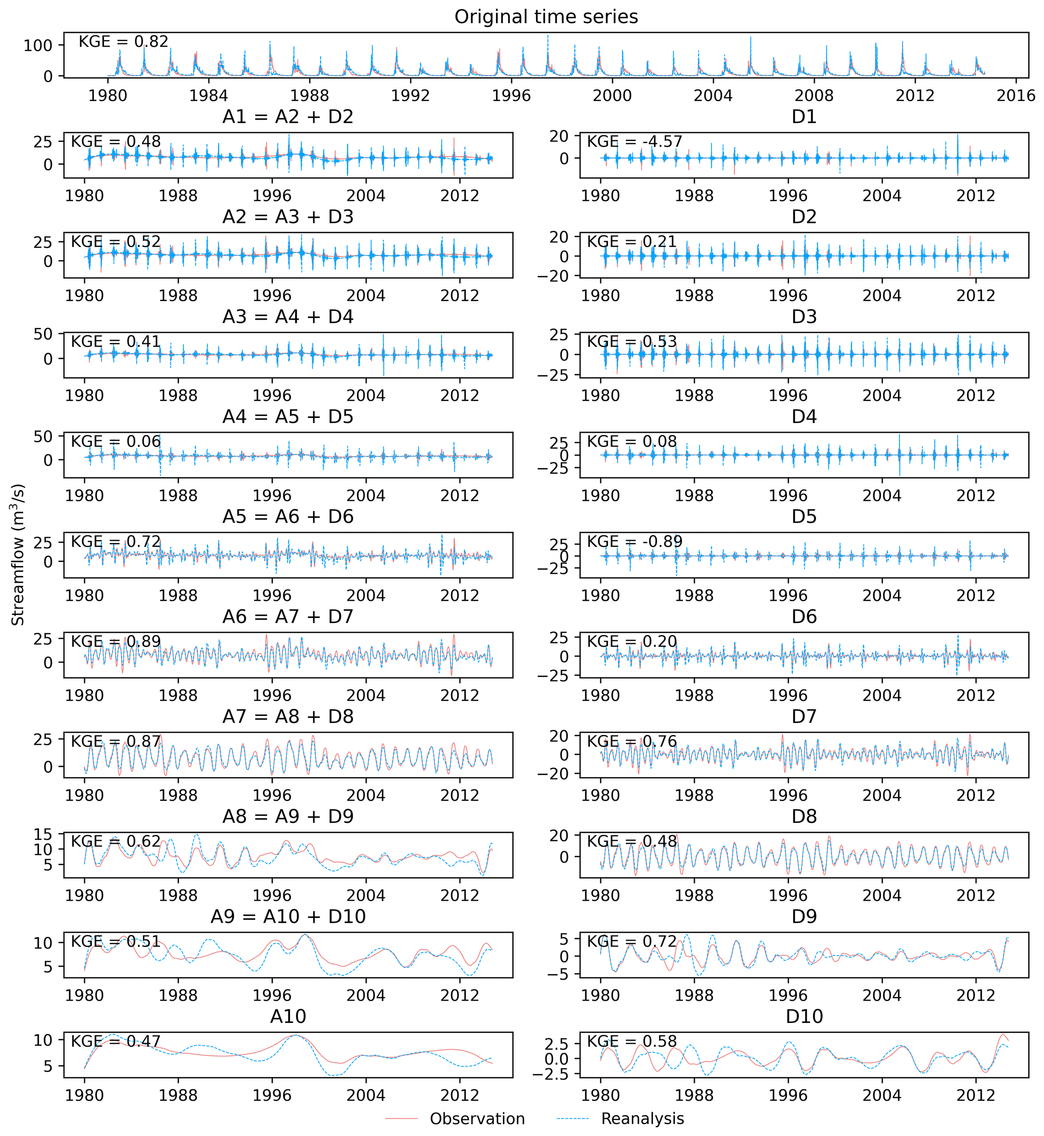
Figure 1 Time series plots of original time series and its approximation and detail components for station 6224000.

The KGEs of approximation and detail components across the CONUS are illustrated in Fig. 2. There are respectively 554 and 417 catchments for the approximation and detail components after removing the outliers. It can be observed that the KGEs of the approximation components tend to increase from A₁ to A₁₀ and that, by contrast, the KGEs of the detail components exhibit considerable fluctuations from D₁ to D₁₀. The comparison between the left and right parts of Fig. 2 highlights that the detail components are more difficult to be characterized than the approximation components. This outcome is attributable to the presence of environmental noise in the original time series (de Macedo Machado Freire et al., 2019). Given that the KGEs of the detail components can drop below −2.5 in some catchments, more attention is paid to the approximation components in the subsequent analysis.

Figure 2 The KGEs of approximation and detail components across the CONUS.

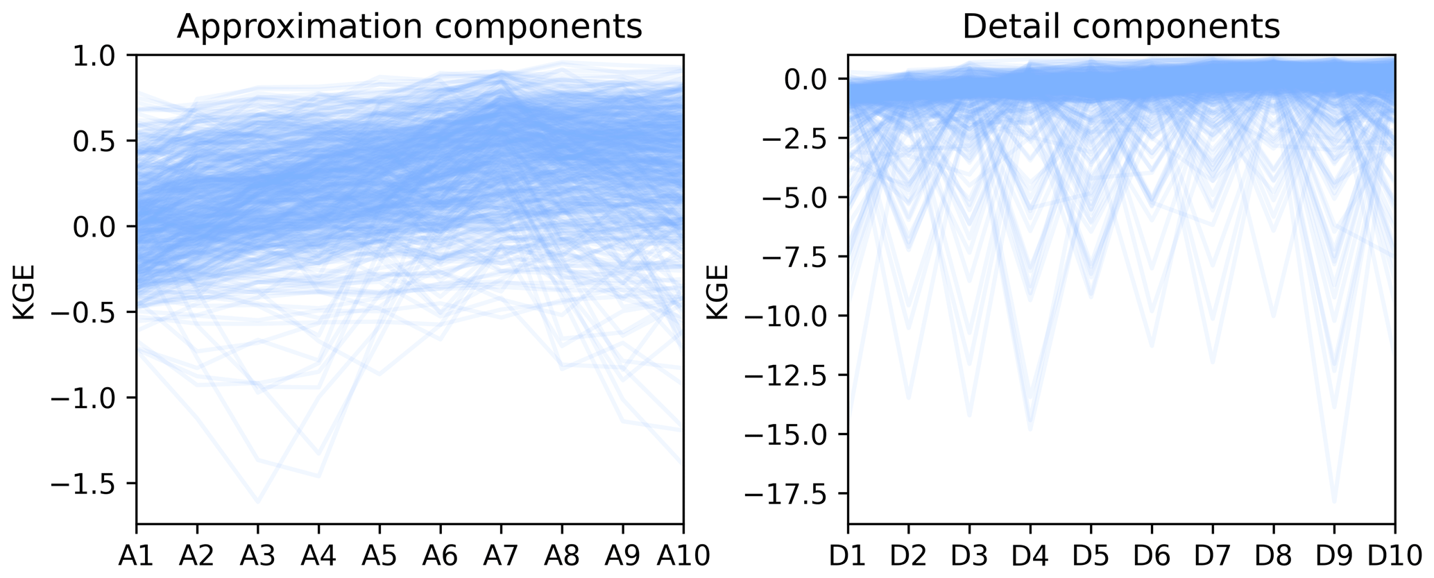
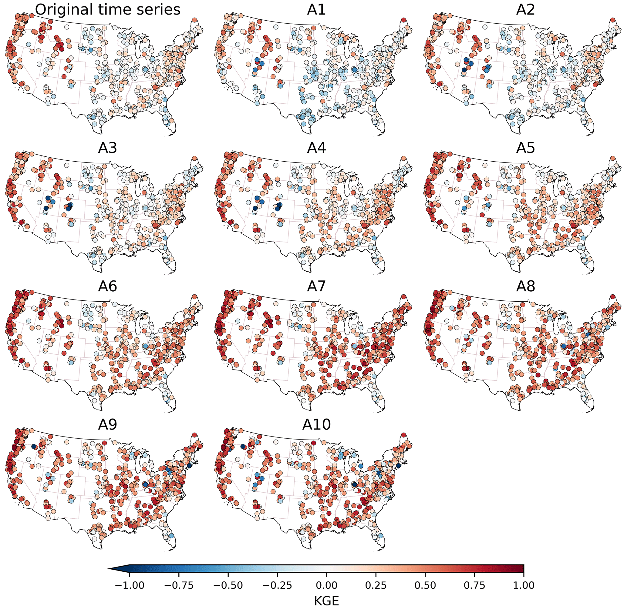
Figure 3 Spatial distribution of the KGE values of original time series and its approximation components from A₁ to A₁₀.

4.2 Performance across the CONUS

The KGE values of original time series and its approximation components for the 554 catchments after removing the outliers are presented in Fig. 3. In total, there are 11 spatial plots for original time series and its components after decomposition. It can be observed that the original time series tends to exhibit relatively high KGEs in the western United States and relatively low KGEs in the central United States. This observation is consistent with those by Addor et al. (2017), who found poor performances in the high plains and deserts of the southwest. In the meantime, the approximation components from A₁ to A₁₀ tend to exhibit high KGEs in the western United States and low KGEs in the central United States. This finding indicates that the KGE values of approximation components are related to the KGE values of original time series. Moreover, as the scale increases from A₁ to A₁₀, the performance of approximation components tends to improve. The KGEs in the central United States change from negative values in A₁ to positive values in A₁₀. That is, seasonal, annual and multi-annual features tend to be better represented by streamflow reanalysis than daily, weekly and monthly features.

The KGE and its three components for the 554 catchments are illustrated by boxplots in Fig. 4. For the KGEs between streamflow reanalysis and observations, it can be observed that the local performance of streamflow reanalysis generally improves from A₁ to A₇ and then remains promising from A₈ to A₁₀. Specifically, the median value of KGE is 0.02 for A₁, 0.09 for A₂, 0.19 for A₃, 0.24 for A₄, 0.29 for A₅, 0.36 for A₆, 0.47 for A₇, 0.43 for A₈, 0.42 for A₉ and 0.40 for A₁₀. This trend is due to the fact that the correlation ratio tends towards 1 from A₁ to A₇. In the meantime, it is noted that A₇ exhibits higher KGE than the original time series. This result implies that errors in the original time series primarily stem from daily, weekly and monthly components. Focusing on the correlation, the medians of correlation for approximation components exceed 0.2, implying valuable information in multiple timescale approximations. The bias ratio remains nearly constant at each scale for approximation components. That is, the mean values of approximation components are generally similar to the mean values of the original time series.

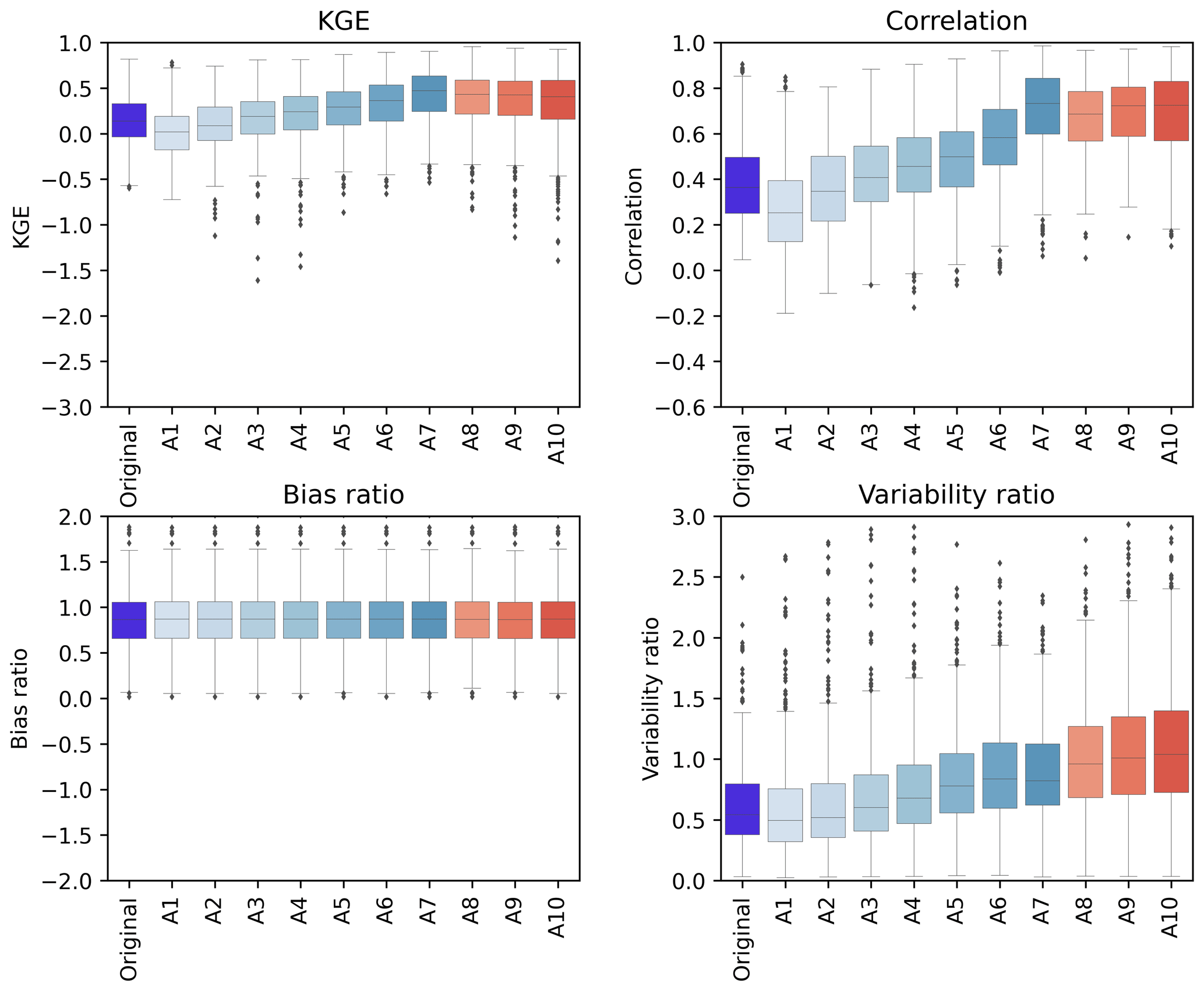
Figure 4 Boxplots of the KGE and its three components for the original time series and its approximation components across 554 catchments in the CONUS. The lines within the boxes mark the median values. The boxes illustrate the interquartile range (IQR), where the lower and upper boundaries of the boxes respectively indicate the lower quartile (Q₁) and upper quartile (Q₃). The lower and upper whiskers show the smallest and largest values within the range of Q₁−1.5IQR to Q₃+1.5IQR. Dark grey diamonds represent outliers that lie beyond the whiskers.

4.3 Influences of catchment attributes

The influences of catchment attributes on the KGE and its three components are measured by the mean absolute ALEs and illustrated in Fig. 5. From the first row, it can be observed that the KGE values of original time series and its approximation components are primarily influenced by precipitation seasonality. Positive (negative) values of precipitation seasonality indicate that precipitation peaks in summer (winter). That is, the season with more precipitation has a significant impact on the KGE. Longitude and mean slope also have a significant impact on the KGE across original time series and daily, weekly, and monthly features (from A₁ to A₅). In the meantime, the correlations of annual and multi-annual features (from A₇ to A₁₀) are mainly affected by the precipitation seasonality, while daily, weekly and monthly features are influenced by longitude and mean slope of the catchment. This result suggests that the influences of catchment attributes on correlation of annual and multi-annual features are different from daily, weekly and monthly features. Furthermore, the bias ratio is primarily influenced by mean precipitation, and the variability ratio is mainly affected by catchment area and depth to bedrock. The geology, soils and vegetation appear to have minor impacts on the local performance of global streamflow reanalysis.

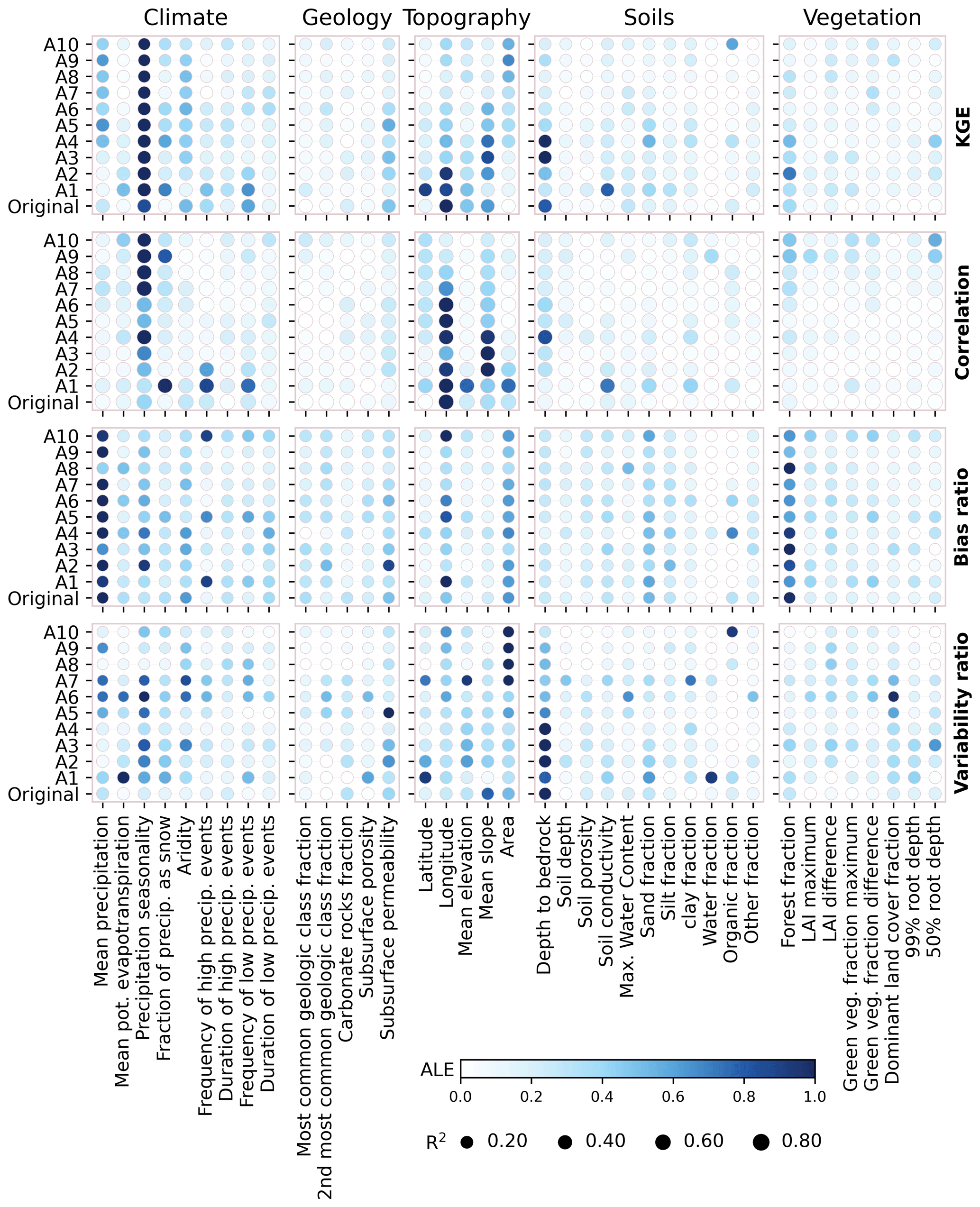
Figure 5 The ALEs of the catchment attributes on the KGE, correlation, bias ratio and variability ratio. The color denotes the mean absolute values for each ALE curve, which is normalized for each original time series (approximation component). The sizes of point represent prediction accuracy indicated by R² for the random forest model using testing set. The “Original” represents original time series.

To further illustrate how catchment attributes affect the performances of original time series and its approximation components, the ALE curves are presented for the three influential attributes of precipitation seasonality, mean precipitation and mean slope of catchment. The influences of precipitation seasonality on the KGE and its three components are presented in Fig. 6. It can be observed that the relationships between the KGE and precipitation seasonality are generally nonlinear. The KGE gradually decreases with the increasing precipitation seasonality. That is, the KGE values are notably low when precipitation tends to concentrate in summer and turn out to be high when precipitation tends to concentrate in winter. The ALE curves of the daily, weekly and monthly features (from A₁ to A₅) are similar to original time series, reducing towards −0.5. The seasonal, annual and multi-annual features (from A₆ to A₁₀) decrease around 0. In the meantime, the influences of precipitation seasonality on the correlation, bias and variability ratios are similar to that on the KGE. These results can be due to low evaporation in winter that results in reasonable simulations of soil moisture and baseflow processes (Poncelet et al., 2017).

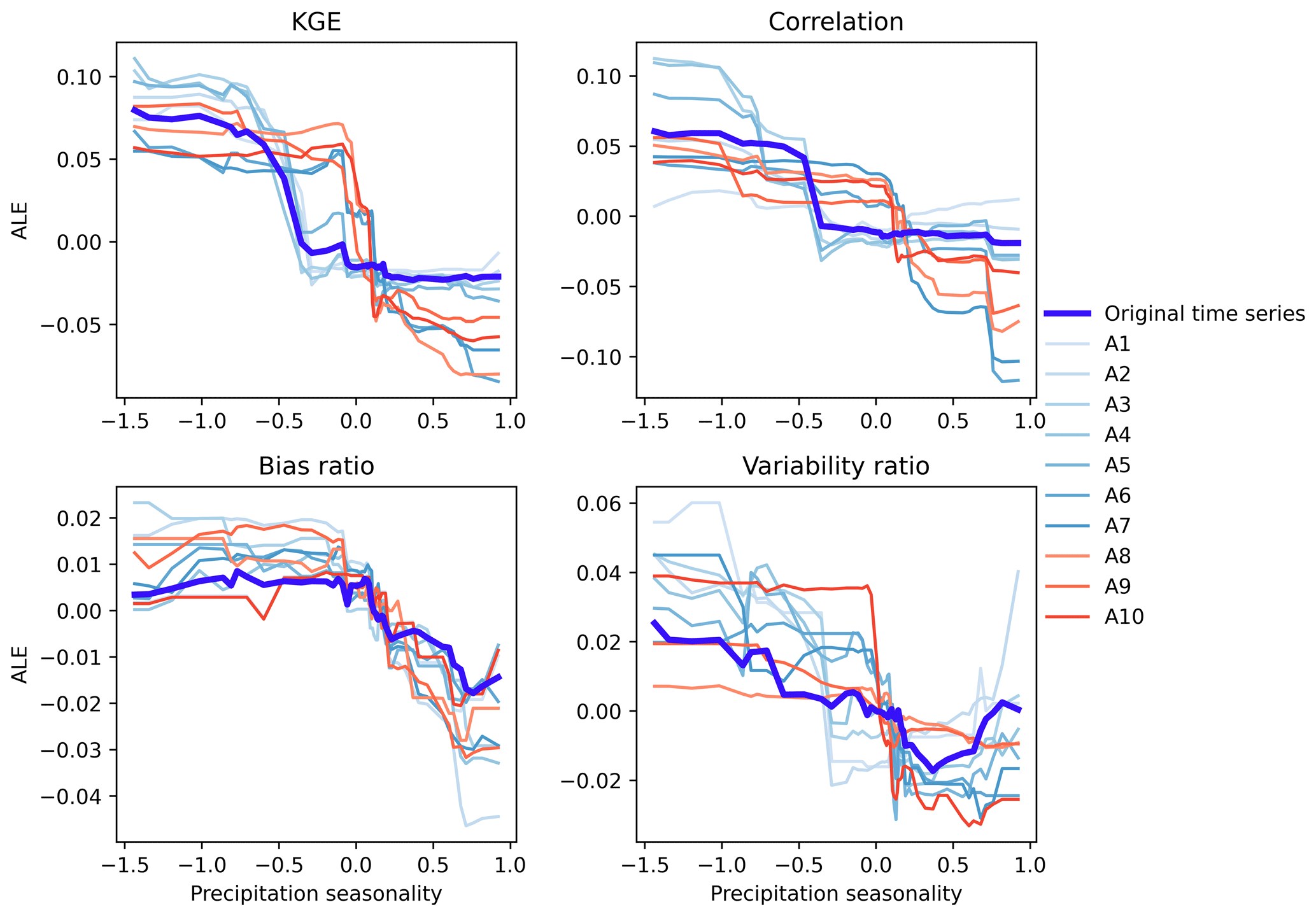
Figure 6 The ALE curves of the relationship between precipitation seasonality and the KGE, correlation, bias ratio and variability ratio for original time series and its approximation components.

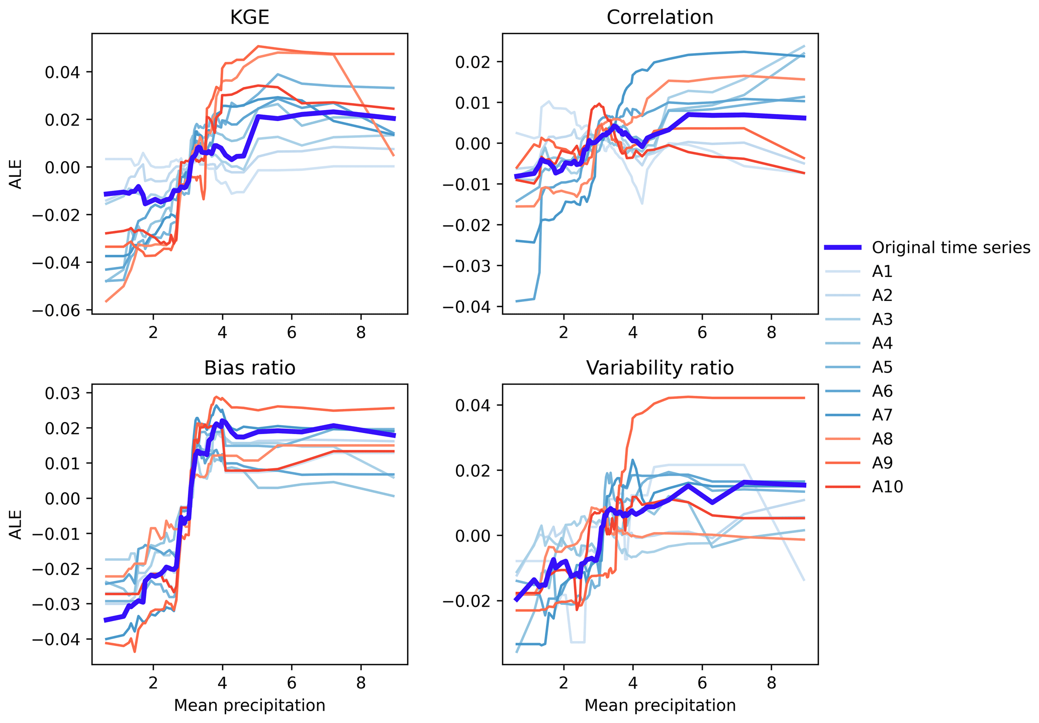
The influences of mean precipitation on the KGE, correlation, bias ratio and variability ratio across different scales are illustrated in Fig. 7. The mean precipitation has a positive effect on the KGE of original time series and its approximation components, with a nonlinear increase of the KGE with rising mean precipitation, particularly for the annual and multi-annual features. In the meantime, it affects the correlation, bias ratio and variability ratio of original time series positively. This result suggests that mean precipitation tends to have a consistent influences on the KGE, correlation, bias and variability ratios for the approximation components. This result can be due to the fact that rainfall–runoff processes are more linear in humid catchments than in arid catchments, leading to less variability in hydrologic states and facilitating more accurate simulations (Parajka et al., 2013).

Figure 7 Same as for Fig. 6 but for mean precipitation.

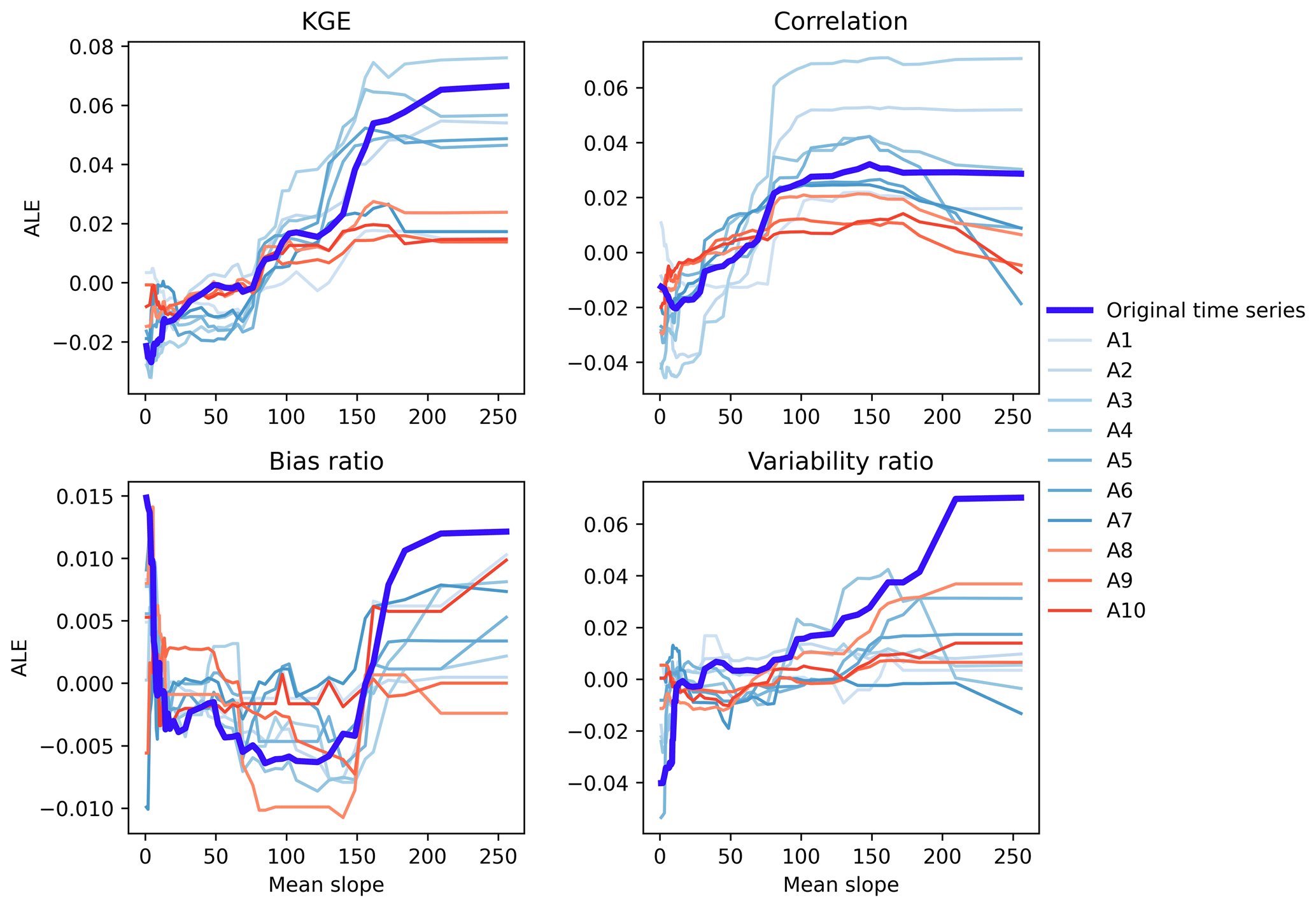
The influences of mean slope on the KGE and its three components across different scales are shown in Fig. 8. It can be observed that there is a nonlinear relationship between the KGE and mean slope of catchment. As the mean slope increases, the KGE of original time series and its approximation components tend to increase. This result may be due to the mean slope of catchment affecting the simulation of runoff generation and infiltration (Stein et al., 2021; Massmann, 2020). It is noted that the KGE values of approximation components gradually increase when the mean slope of catchment surpasses 150. In particular, the correlation and variability ratio of original time series generally increase with the increase in the KGE. That is, the mean slope of catchment has a similar effect on the KGE, correlation and variability ratio. On the other hand, bias ratio initially decreases and then increases with the increase of mean slope. In other words, the relationship between bias ratio and mean slope of catchment is non-monotonic.

Figure 8 Same as for Fig. 6 but for mean slope.

4.4 Driving factors of each catchment

The most important attribute that influences the KGE is identified for each catchment by the LIMEs method and then illustrated by spatial plots in Fig. 9. It can be observed that the most important attributes influencing the KGE exhibit regional clustering. The KGE of original time series is primarily influenced by precipitation seasonality in the western and central United States and by depth to bedrock in the eastern United States (Addor et al., 2017; Pfister et al., 2017). The substantial differences in precipitation seasonality between the western and central United States result in significant differences in the KGE. On the other hand, the most important attribute controlling the KGE of approximation components is different from that of original time series. It can be observed that the KGE values of approximation components from A₆ to A₈ are primarily controlled by precipitation seasonality in the eastern United States, while the original time series is controlled by depth to bedrock. The higher depth to bedrock may exhibit larger storage values, consequently leading to higher baseflow (Pfister et al., 2017). In the meantime, the number of catchments controlled by precipitation seasonality tends to increase from A₁ to A₈, with a high proportion observed in A₆, A₇ and A₈. That is, the performance of the annual variability of streamflow reanalysis is influenced by precipitation seasonality.

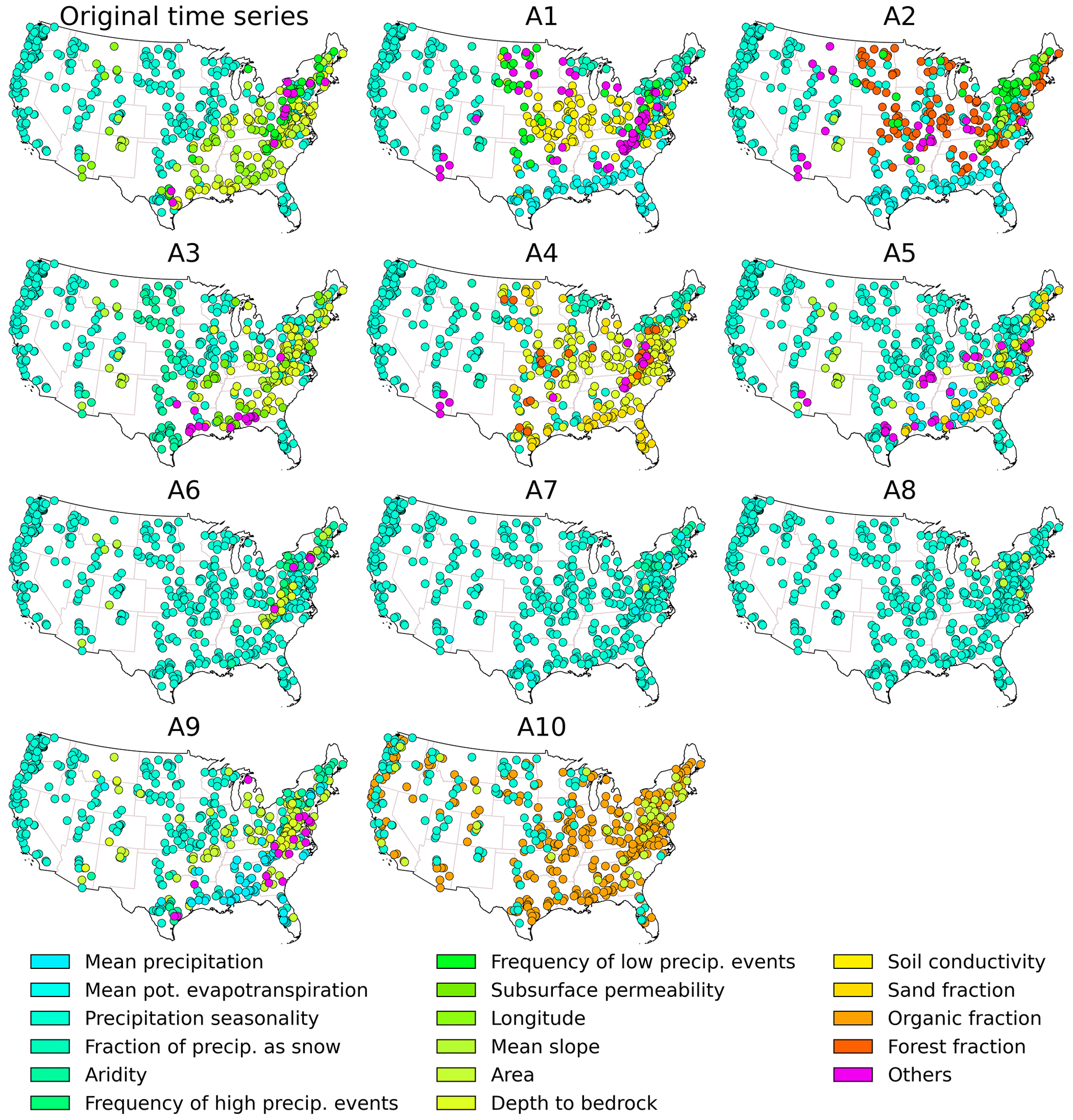
Figure 9 Spatial patterns of the controlling catchment attribute on the KGE of original time series and approximation components for each catchment. For each spatial distribution map, if there are more than five catchment attributes, only the top five attributes are presented, while the rest are labeled as others.

5 Discussion

Global streamflow reanalysis provides valuable information for water resources management (Alfieri et al., 2020; Harrigan et al., 2020; Yang et al., 2021). Building upon previous studies evaluating the performance of hydrological signatures derived from reanalysis and observed streamflow (Beck et al., 2017; Chen et al., 2021; Tu et al., 2024), this paper presents a novel evaluation by combining the wavelet transform with machine learning. Specifically, streamflow reanalysis and observation are respectively decomposed by the DWT into detail and approximation components at different scales. As a result, streamflow characteristics in the time–frequency domain are unraveled by extracting features and removing noise from the original signal (Manikanta and Vema, 2022). This approach provides a new perspective by paying attention to the difference between global streamflow reanalysis and observed streamflow in the time–frequency domain. The KGE generally indicates that streamflow reanalysis exhibits a robust capability to capture the information of seasonal, annual and multi-annual variability, particularly the annual fluctuations. This result suggests that hydrological simulations at daily or even hourly timescales are more challenging.

Hydrological models generally exhibit different performances across different catchments (Newman et al., 2015; O'Neill et al., 2021; Tu et al., 2024). The differences can be related to heterogeneous streamflow patterns under unique combinations of climate and catchment attributes (Stein et al., 2021). Previous studies have found that model performance is related to aridity index, with generally better performance in wetter catchments compared to drier ones (Poncelet et al., 2017). In addition to aridity index, other factors are also linked to the model performance, such as impact of snow (Newman et al., 2015), catchment area (Harrigan et al., 2020), precipitation intermittency (Newman et al., 2015) and human activities (Veldkamp et al., 2018). In this paper, it is found that the KGE values of original time series and approximation components are primarily influenced by precipitation seasonality. This outcome can be due to lower evaporation in winter, when the soil moisture is higher and baseflow can be better simulated (Poncelet et al., 2017). On the other hand, the relationships between KGE and catchment attributes are nonlinear. The results highlight that the wavelet transform can facilitate the evaluation of the local performance of global streamflow reanalysis to provide more effective information.

6 Conclusions

This paper has presented a novel decomposition approach to evaluating global streamflow reanalysis by combining the widely used wavelet transform and machine learning techniques. Specifically, the reanalysis and observed streamflow are decomposed by the DWT, and then they are used to indicate the local performance of the time series characteristics in the time–frequency domain. Furthermore, the influences of catchment attributes on the performance of original time series and its approximation components at various scales are investigated using the ALEs. A large-sample test is conducted for the CAMELS dataset so as to evaluate the effectiveness of GloFAS streamflow reanalysis. The results show that the streamflow reanalysis tends to characterize seasonal, annual and multi-annual variabilities more efficiently than daily, weekly and monthly variabilities. Precipitation seasonality is identified to be the most important attribute influencing the KGE of original time series and its approximation components using the ALEs. The longitude, mean precipitation and mean slope also influence the performance of approximation components. On the other hand, the attributes on geology, soils and vegetation seem to have a relatively minor influence on the performance of approximation components. Overall, the evaluation of global streamflow reanalysis at different timescales using decomposition approaches provides useful information for practical applications of global streamflow reanalysis.