Skill of seasonal flow forecasts at catchment scale: an assessment across South Korea

Recent advancements in numerical weather predictions have improved forecasting performance at longer lead times. Seasonal weather forecasts, providing predictions of weather variables for the next several months, have gained significant attention from researchers due to their potential benefits for water resources management. Many efforts have been made to generate seasonal flow forecasts (SFFs) by combining seasonal weather forecasts and hydrological models. However, producing SFFs with good skill at a finer catchment scale remains challenging, hindering their practical application and adoption by water managers. Consequently, water management decisions in both South Korea and numerous other countries continue to rely on worst-case scenarios and the conventional ensemble streamflow prediction (ESP) method.

This study investigates the potential of SFFs in South Korea at the catchment scale, examining 12 reservoir catchments of varying sizes (ranging from 59 to 6648 km²) over the last decade (2011–2020). Seasonal weather forecast data (including precipitation, temperature and evapotranspiration) from the European Centre for Medium-Range Weather Forecasts (ECMWF SEAS5) are used to drive the Tank model (conceptual hydrological model) to generate the flow ensemble forecasts. We assess the contribution of each weather variable to the performance of flow forecasting by isolating individual variables. In addition, we quantitatively evaluate the “overall skill” of SFFs, representing the probability of outperforming the benchmark (ESP), using the continuous ranked probability skill score (CRPSS). Our results highlight that precipitation is the most important variable in determining the performance of SFFs and that temperature also plays a key role during the dry season in snow-affected catchments. Given the coarse resolution of seasonal weather forecasts, a linear scaling method to adjust the forecasts is applied, and it is found that bias correction is highly effective in enhancing the overall skill. Furthermore, bias-corrected SFFs have skill with respect to ESP up to 3 months ahead, this being particularly evident during abnormally dry years. To facilitate future applications in other regions, the code developed for this analysis has been made available as an open-source Python package.

1 Introduction

Over the last decade, numerical weather prediction systems have improved their forecasting performance at longer lead times ranging from 1 to several months ahead (Bauer et al., 2015; Alley et al., 2019). The water management sector may benefit considerably from these advances. In particular, predictions of weather variables such as precipitation and temperature several months ahead (from now on referred to as seasonal weather forecasts) might be exploited to anticipate upcoming dry periods and implement management strategies for mitigating future water supply deficits (Soares and Dessai, 2016).

To increase relevance for water resource management, seasonal weather forecasts can be translated into seasonal flow forecasts (SFFs) via a hydrological model. SFFs can be provided and evaluated at different temporal and spatial resolutions: a coarser resolution, e.g. magnitude of total next-month runoff over a certain region (Prudhomme et al., 2017; Arnal et al., 2018), or a finer resolution, e.g. daily/weekly flow at a particular river section over the next month (Crochemore et al., 2016; Lucatero et al., 2018). This distinction is important here because coarser-resolution SFFs can only be applied to inform water management in a qualitative way, whereas finer-resolution SFFs can also be used to force a water resource system model for a quantitative appraisal of different management strategies. Proof-of-principle examples of the latter approach are provided by Chiew et al. (2003), Boucher et al. (2012) and Peñuela et al. (2020). These papers have demonstrated, through model simulations, the potential of using SFFs to improve the operation of supply reservoirs (Peñuela et al., 2020), irrigation systems (Chiew et al., 2003) and hydropower systems (Boucher et al., 2012).

Obviously, generating SFFs with good skill at finer scales is challenging and the lack of forecast performance is often cited as a key barrier to real-world applications of SFFs by water managers (Whateley et al., 2015; Soares and Dessai, 2016; Jackson-Blake et al., 2022). In practice, if a water resource system (WRS) model is used to simulate and compare different operational decisions, this is done by forcing the WRS model to repeat of a historical low flow event (“worst-case” scenario) (Yoe, 2019) or against the ensemble streamflow prediction (ESP). ESP is a widely used operational forecasting method whereby an ensemble of flow forecasts is generated by forcing a hydrological model by historical meteorological observations (Day, 1985; Baker et al., 2021). Since the hydrological model is initialized at current hydrological conditions, ESP is expected to have a certain level of performance, particularly in “long-memory” systems, where the impact of initial conditions last over long time periods (Li et al., 2009). Previous simulation studies that examined the use of SFFs to enhance the operation of WRS (e.g. Peñuela et al., 2020, as cited above) did indeed show that ESP serves as a hard-to-beat benchmark. Similar to other countries, in South Korea, the worst-case scenario and ESP are used to inform water management activities, whereas SFFs are not currently applied. Before the use of SFFs can be proposed to practitioners, it is thus crucial to understand the skill of such products with respect to ESP.

Numerous studies have been conducted on the skill of SFFs in different regions of the world. Some of these studies focused on the “theoretical skill”, which is determined by comparing SFFs with pseudo-observations produced by the same hydrological model when forced by observed temperature and precipitation. This experimental setup enables the isolation of the contribution of the weather forecast skill to the flow forecast skill, regardless of structural errors that may be present in the hydrological model. In general, most studies have found that the theoretical skill of SFFs may be only marginally better than that of ESP in specific regions and lead time. For example, Yossef et al. (2013) analysed multiple large river basins worldwide and found that SFFs generally perform worse than ESP. Likewise, the findings of Greuell et al. (2019) indicated that SFFs are more skilful than ESP for the first lead month only. Across Europe, the theoretical skill of SFFs was found to be higher than ESP in coastal and mountainous regions (Greuell et al., 2018).

Although important to how the information content of seasonal weather forecasts varies across regions with different climatic characteristics, from a water management perspective, the theoretical skill may not be the most appropriate metric, as it reflects the performance within the modelled environment (Pechlivanidis et al., 2020) rather than the real world. The “actual skill”, which is determined by comparing SFFs to flow observations, would be more informative for water managers to decide on whether to use SFFs and when. Previous studies that investigated the actual skill showed that, as expected, the actual skill is lower than the theoretical skill due to errors in the hydrological model and in the weather input observations (Van Dijk et al., 2013; Greuell et al., 2018).

In addition, due to the coarse horizontal resolution of seasonal weather forecasts, particularly of precipitation forecasts, the forecast skill can be significantly improved through bias correction (e.g. Crochemore et al., 2016; Lucatero et al., 2018; Tian et al., 2018). However, even after bias correction, SFFs were found to be unable to surpass ESP in many previous applications (e.g. Crochemore et al., 2016; Lucatero et al., 2018; Greuell et al., 2019).

Previous studies reviewed above have mainly used the seasonal weather forecasts provided by the European Centre for Medium-Range Weather Forecasts (ECMWF). Here, it is important to note that the majority of these studies have utilized ECMWF's System 3 (e.g. Yossef et al., 2013) or 4 (e.g. Crochemore et al., 2016; Lucatero et al., 2018; Tian et al., 2018; Greuell et al., 2019). A few studies comparing the performance of SFFs and ESP have been conducted based on ECMWF's cutting-edge forecasting system SEAS5, which became operational in November 2017. These include Peñuela et al. (2020) and Ratri et al. (2023), which, however, did not analyse the skill of SFFs in much detail but rather focused on their operational implementation. Given that the upgrade of forecasting systems can lead to substantial enhancement in the performance (e.g. Johnson et al., 2019; Köhn-Reich and Bürger, 2019), it is interesting to assess whether the improved skill of weather forecasts delivered by SEAS5 translates into the improved skill of flow forecasts.

Our previous research (Lee et al., 2023) on the skill of seasonal precipitation forecasts across South Korea showed that, among various forecasting centres, ECMWF provides the most skilful seasonal precipitation forecasts, outperforming the climatology (based on historical precipitation observations). This is particularly evident during the wet season (June to September) and in dry years, where skill can also be high at longer lead times beyond the first month.

Building on these previous findings, this study aims to investigate the performance of SFFs compared to ESP in predicting flow. Specifically, we focus on 12 catchments of various sizes (from 59 to 6648 km²), which include the most important multipurpose reservoirs across South Korea and where the use of SFFs may be considered for assisting operational decisions and mitigating impacts of droughts. Given this practical long-term goal, our study focuses on assessing the “overall skill”, which represents the long-term probability that SFFs outperform the benchmark (ESP) when comparing the flow forecasts with historical flow observations. As a hydrological model, we use the lumped Tank model (Sugawara et al., 1986) which is the rainfall-runoff model currently in use for national water management and planning. For all catchments, we briefly analyse the hydrological model performance and also investigate which weather forcing input (precipitation, temperature and potential evapotranspiration) contributes most to the performance of SFFs across different catchments before and after bias correction. Finally, we look at how the overall skill varies across seasons, years and catchments to draw conclusions on when and where SFFs may be more informative than ESP for practical water resources management. In doing so, we develop a workflow for SFFs analysis implemented in a Python Jupyter Notebook, which can be utilized by other researchers for evaluating and testing SFFs in various regions.

2 Material and methodology

2.1 Study site and data

2.1.1 Study site

The spatial scope of this study is defined as the catchments upstream of 12 multipurpose reservoirs across South Korea. While there are 20 multipurpose reservoirs nationwide (K-water, 2022), we have specifically selected 12 reservoirs with at least 10 years of flow observation and no external flows from other rivers or reservoirs. The locations of the catchments and the mean annual precipitation, temperature and potential evapotranspiration (PET) are shown in Fig. 1a–c. The weather data for the selected reservoir catchments are reported in Table 1.

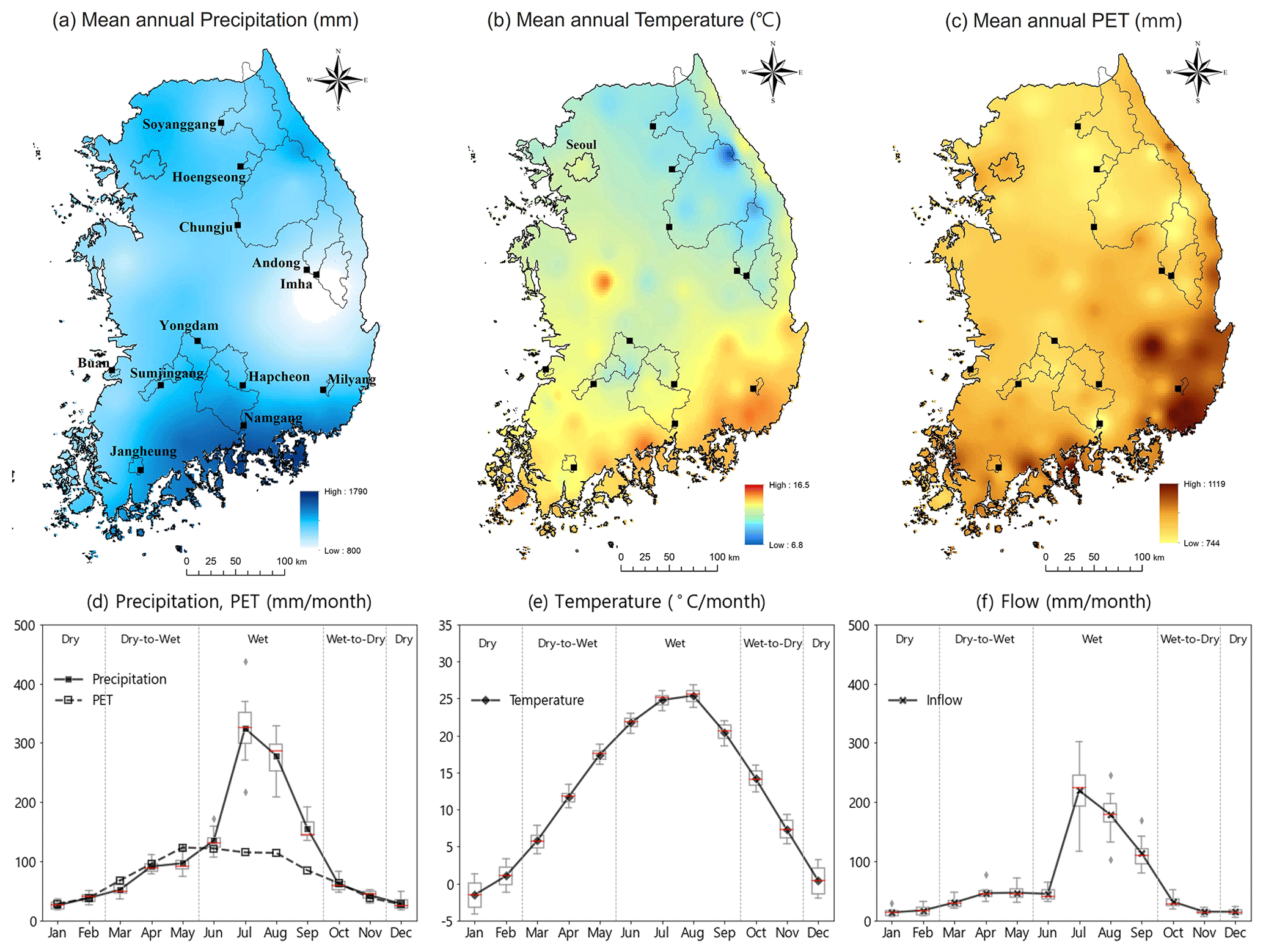
Figure 1 Top row shows mean annual (a) precipitation, (b) temperature and (c) PET across South Korea over the period 1967–2020. Black lines are the boundaries of the 12 reservoir catchments analysed in this study (all maps obtained by interpolating point measurements using the inverse distance weighting method). Bottom row shows (d) cumulative monthly precipitation and PET, (e) mean monthly temperature, and (f) cumulative monthly flow. These three variables are averaged over the 12 reservoir catchments from 2001 to 2020. Boxplots show the inter-catchment variability.

Table 1 Characteristics of the 12 multipurpose reservoirs (from north to south) and the catchments they drain (K-water, 2022). T_min and T_max represent mean monthly minimum and maximum temperatures averaged over 2001–2020, and all other meteorological variables (P: precipitation, T: temperature, PET: potential evapotranspiration) are annual averages over the same period.

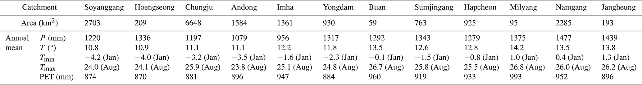
Figure 1d–f shows the monthly precipitation and PET (Fig. 1d), temperature (Fig. 1e), and flow (Fig. 1f), averaged over the 12 selected catchments for the period 2001 to 2020. Generally, the catchments located in the southern region exhibit higher mean annual precipitation, temperature, and PET. In order to examine how the skill of seasonal weather and flow forecasts varies across a year, we divide the year into four seasons based on monthly precipitation (Lee et al., 2023): dry season (December to February), dry-to-wet transition (March to May), wet season (June to September) and wet-to-dry transition (October to November). As shown in this figure, most of the total annual precipitation (and the corresponding flow) occurs during the hot and humid wet season, while the dry season is characterized by cold and dry conditions. Figure 1d–f also shows high inter-catchment variability during the wet season in both precipitation (Fig. 1d) and flow (Fig. 1f), whereas the inter-catchment variability in temperature (Fig. 1e) is more obvious during the dry season. Additionally, there is a high inter-annual variability in precipitation and flow in South Korea, which is attributed to the impacts of typhoons and monsoons (Lee et al., 2023).

2.1.2 Hydrological data and seasonal weather forecasts

Precipitation, temperature and potential evapotranspiration are the key variables required to simulate flow using a hydrological model. To this end, daily precipitation data from 1318 in situ stations from the Ministry of Environment; the Korea Meteorologic Administration (KMA); and the national water resources agency, the Korea Water Resources Corporation (K-water) (Ministry of Environment, 2021) and daily temperature data from 683 in situ stations from the KMA were obtained. Both precipitation and temperature data cover the period from 1967 to 2020 (see Fig. 1). Potential evapotranspiration (PET) data were computed using the standardized Penman–Monteith method suggested by the UN Food and Agriculture Organization (Allen et al., 1998). The precipitation and temperature measurements have been quality-controlled by the Ministry of Environment. We used the Thiessen polygon method to calculate the catchment average precipitation and temperature.

The flow data used in this study refer to the flow into the reservoir from its respective upstream catchment (see Table 1 and Fig. 1). K-water generates daily inflow data using a water-balance equation, which takes into account the daily changes in reservoir volume (from the storage-elevation curve) caused by the water level fluctuations and releases from the reservoir. However, to date, reservoir evaporation has not been considered in the flow estimation process. In this study, quality-controlled daily flow data for each reservoir produced by K-water are used.

Several weather forecasting centres, including ECMWF, UK Met Office and German Weather Service, provide seasonal weather forecast datasets through the Copernicus Climate Data Store (CCDS). According to our previous study (Lee et al., 2023), ECMWF was found to be the most skilful provider of seasonal precipitation forecasts for South Korea. Since precipitation is one of the most important weather forcings in hydrological forecasting (Kolachian and Saghafian, 2019), we have utilized the seasonal weather forecast datasets from ECMWF SEAS5 (Johnson et al., 2019) in this study. Since 1993, ECMWF has been providing 51 ensemble forecasts (a set of multiple forecasts that are equally as likely) on a monthly basis (25 ensembles prior to 2017) with a horizontal resolution of 1°×1° and daily temporal resolution of up to 7 months ahead. In this study, the time period from 1993 to 2020 was selected and the ensemble forecasts for the selected catchments were downloaded from the CCDS. Here, we utilized data from 1993 to 2010 to generate bias correction factors and data from 2011 to 2020 to assess the skill (see Fig. S1 in the Supplement).

2.2 Methodology

The methodology of our analysis is summarized in the schematic diagram shown in Fig. 2. Firstly, we compiled a seasonal weather forecast ensemble from ECMWF for precipitation (P), temperature (T) and PET over the 12 reservoirs for 10 years, from 2011 to 2020. To downscale the datasets, a linear scaling method was applied to each weather forcing (Sect. 2.2.1). Secondly, we estimated the parameters of the hydrological model and validated its performance (Sect. 2.2.2). Utilizing the seasonal weather forecast dataset as input data to the hydrological model, we generated an ensemble of SFFs, and using historical weather observations as input, we produced ESP. Specifically, to calculate ESP, 45 ensemble members of each weather variable were also selected from historical observations (1966–2010; see Fig. S1). Each ensemble member represents the simulated flow using a hydrological model initialized with observed meteorological data to simulate current conditions and forced by historical meteorological observations for the forecasting period. The continuous ranked probability score (CRPS) and the continuous ranked probability skill score (CRPSS) were applied (Sect. 2.2.3) to calculate the absolute performance (score) of each forecast product (Sect. 3.1 and 3.2) and the relative performance (overall skill) of SFFs with respect to ESP (Sect. 3.3 and 3.4).

Figure 2 Schematic diagram illustrating the analysis method of the study.

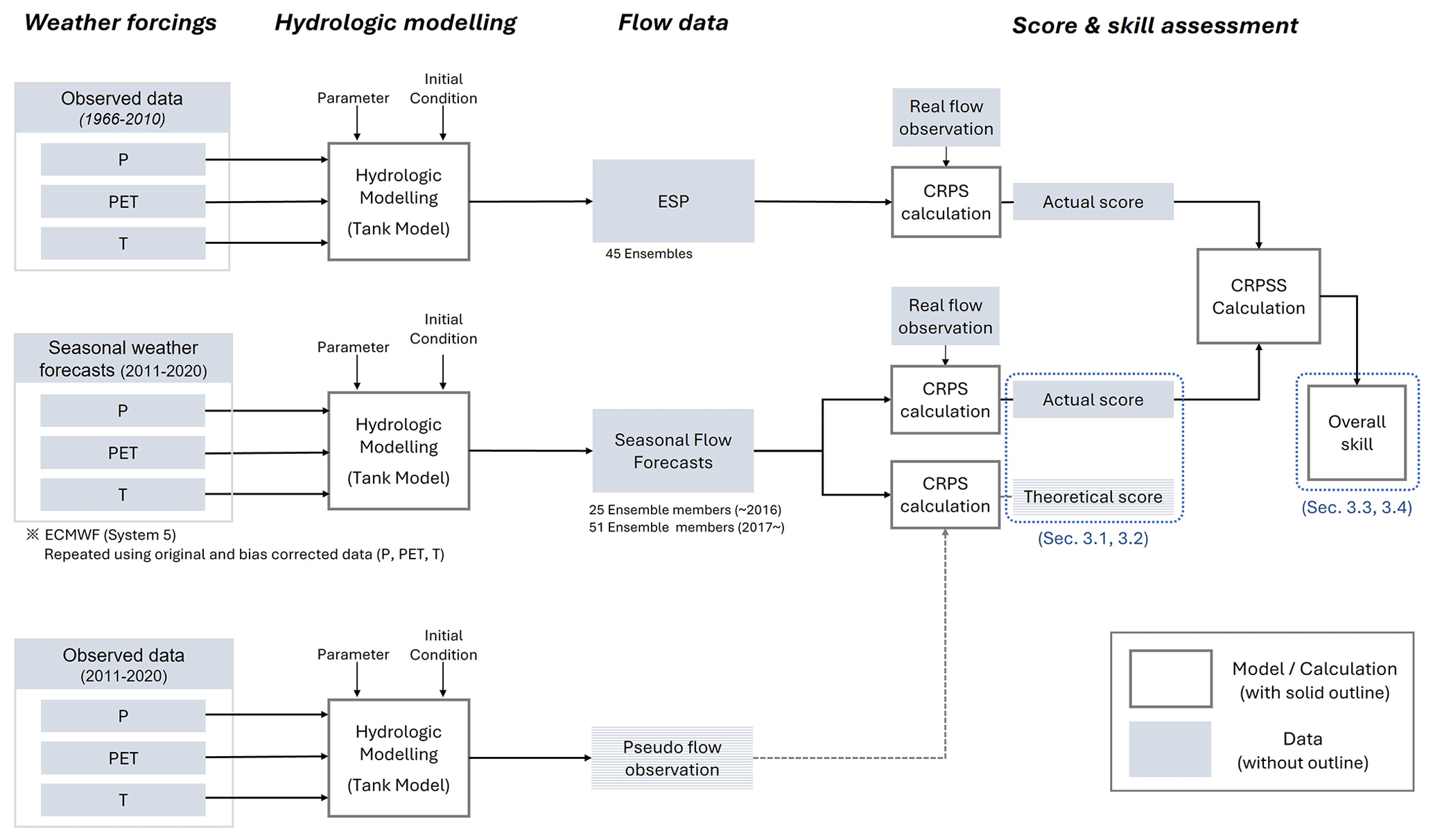
Specifically, in Sect. 3.1, we analyse the contribution of hydrological modelling uncertainty to the performance of SFFs by comparing the actual score calculated using flow observations to the theoretical score calculated using pseudo flow observations. Here, pseudo-observation refers to the flow time series obtained by feeding the hydrological model with weather observations, i.e. where errors due to hydrological model are removed. In Sect. 3.2, we investigate which weather variable mostly influences the performance of SFFs. To do so, we first calculate the “isolated score” of the flow forecasts generated by forcing the hydrological model by seasonal weather forecasts for one meteorological variable while using observational data for the other two variables. For instance, to assess the contribution of precipitation, we calculated the isolated score of precipitation using seasonal precipitation forecasts and observations for temperature and PET. Then, we computed the “integrated score” using seasonal weather forecasts for all three variables and determined the “relative scores” for each variable as the ratio of the isolated score over the integrated score. This workflow is illustrated in Fig. S2. In Sect. 3.3 to 3.5, we examine the regional and seasonal variations and the characteristics of overall skill under extreme climate conditions.

2.2.1 Bias correction (statistical downscaling)

The seasonal weather forecast datasets from CCDS have a spatial resolution of 1°×1°, which is too coarse for the catchment-scale analysis. Previous studies also have reported that seasonal weather forecasts generated from general circulation models contain systematic biases and that this can cause forecast uncertainty (Maraun, 2016; Manzanas et al., 2017; Tian et al., 2018). Moreover, the usefulness of bias correction in enhancing the forecast skill has been shown in many previous studies (Crochemore et al., 2016; Tian et al., 2018; Pechlivanidis et al., 2020; Ferreira et al., 2022). Hence, it is imperative to investigate the potential enhancement in the skill of hydrological forecasts resulting from the bias correction of weather forcings.

Numerous bias correction methods have been developed, including the linear scaling method, local intensity scaling and quantile mapping (Fang et al., 2015; Shrestha et al., 2017). Thanks to its simplicity and low computational cost (Melesse et al., 2019), the linear scaling method is widely adopted. Despite its simplicity, this method has demonstrated practical usefulness in various studies (Crochemore et al., 2016; Shrestha et al., 2017; Azman et al., 2022), including our previous study on seasonal precipitation forecasts across South Korea (Lee et al., 2023). Therefore, the linear scaling method was utilized in this study.

Previous studies found that additive correction is preferable for temperature, whereas multiplicative correction is preferable for variables such as precipitation, evapotranspiration and solar radiation (Shrestha et al., 2016). Consequently, the equations for the linear scaling method for each variable can be expressed as

$$\begin{array}{}\text{(1)}& \begin{array}{rl}{P}_{\mathrm{forecasted}}^{*}& =P_{\mathrm{forecasted}}\cdot {\left(b_{\mathrm{P}}\right)}_{\mathrm{m}}=P_{\mathrm{forecasted}}\\ & \cdot \left[{\displaystyle \frac{{\mathit{\mu }}_{\mathrm{m}}\left(P_{\mathrm{observed}}\right)}{{\mathit{\mu }}_{\mathrm{m}}\left(P_{\mathrm{forecasted}}\right)}}\right],\end{array}\end{array}$$

$$\begin{array}{}\text{(2)}& {\displaystyle }\begin{array}{rl}{\mathrm{PET}}_{\mathrm{forecasted}}^{*}& ={\mathrm{PET}}_{\mathrm{forecasted}}\cdot {\left(b_{\mathrm{PET}}\right)}_{\mathrm{m}}={\mathrm{PET}}_{\mathrm{forecasted}}\\ & \cdot \left[{\displaystyle \frac{{\mathit{\mu }}_{\mathrm{m}}\left({\mathrm{PET}}_{\mathrm{observed}}\right)}{{\mathit{\mu }}_{\mathrm{m}}\left({\mathrm{PET}}_{\mathrm{forecasted}}\right)}}\right],\end{array}\text{(3)}& {\displaystyle }\begin{array}{rl}{T}_{\mathrm{forecasted}}^{*}& =T_{\mathrm{forecasted}}+{\left(b_T\right)}_{\mathrm{m}}=T_{\mathrm{forecasted}}\\ & +\left[{\mathit{\mu }}_{\mathrm{m}}\left(T_{\mathrm{observed}}\right)-{\mathit{\mu }}_{\mathrm{m}}\left(T_{\mathrm{forecasted}}\right)\right]\end{array},\end{array}$$

where $Y_{\mathrm{forecasted}}^{*}$ is the bias-corrected forecast variable Y (such as P, PET and T) at a daily timescale, Y_forecasted is the original forecast variable before bias correction and (b_Y)_m is the bias correction factor for each variable at month m. μ_m represents the monthly mean, and Y_observed is the observed daily data for the variable. In this study, daily precipitation forecasts were bias corrected using the monthly bias correction factor (b_Y)_m for each month (m=1 to 12). The bias correction factor was computed using the observations and original forecast datasets from 1993 to 2010, and these were then applied to adjust each seasonal weather forecast for later years (2011 to 2020).

2.2.2 Hydrological modelling

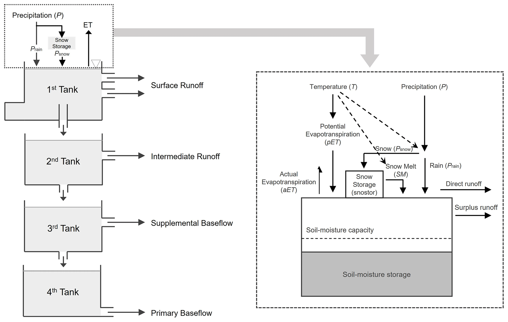
The Tank model was first developed by Sugawara of Japan in 1961 (Sugawara et al., 1986; Sugawara, 1995) and has become a widely used conceptual hydrological model in many countries (Ou et al., 2017; Goodarzi et al., 2020). A modified version of the Tank model, incorporating soil moisture structures and snowmelt modules, is commonly used in South Korea for long-term water resources planning and management purposes due to its good performance (Kang et al., 2004; Lee et al., 2020). As shown in Fig. 3, the modified Tank model used in this study comprises four storage tanks representing the runoff and baseflow in the target catchment (Shin et al., 2010; Phuong et al., 2018) and incorporates a water-balance module suggested by the United States Geological Survey (McCabe and Markstrom, 2007).

Figure 3 The structure of modified Tank model (left) and its water-balance module (right).

This model has 21 parameters (see Table S1 in the Supplement), which were calibrated based on historical observations. We calibrated the model using observations for the period from 2001 to 2010, and the validation was done using the time period from 2011 to 2020. To estimate the model parameters, the Shuffled Complex Evolution (SCE-UA) global optimization algorithm, developed at the University of Arizona (Duan et al., 1992, 1994), is utilized. This algorithm has widely been used for the calibration of hydrological models and has shown more robust and efficient performance compared to many traditional optimization methods, such as genetic algorithm, differential evolution and simulated annealing (Yapo et al., 1996; Rahnamay-Naeini et al., 2019). The following objective function (OF), proposed by Sugawara (Sugawara et al., 1986), is applied for the SCE-UA algorithm because a previous study demonstrated that this objective function generally shows superior results in calibrating the Tank model in South Korean catchments with calibration periods longer than 5 years (Kang et al., 2004):

$$\begin{array}{}\text{(4)}& \mathrm{OF}=\sum _{t=\mathrm{1}}^N\left|q_t^{\mathrm{obs}}-q_t^{\mathrm{sim}}\right|/q_t^{\mathrm{obs}},\end{array}$$

where t and N represent time (in days) and total number of time steps and $q_t^{\mathrm{obs}}$ and $q_t^{\mathrm{sim}}$ represent the observed and simulated flow at time t, respectively. The optimal parameter set is the one that produces the lowest value from the objective function.

In order to evaluate the model performance in diverse perspectives, we used three different evaluation indicators: Nash–Sutcliffe efficiency coefficient (NSE), percentage bias (PBIAS) and ratio of volume (ROV). The calculation of each indicator was carried out as described by the following equations:

$$\begin{array}{}\text{(5)}& {\displaystyle }& {\displaystyle }\mathrm{NSE}=\mathrm{1}-\sum _{t=\mathrm{1}}^N{\left(q_t^{\mathrm{obs}}-q_t^{\mathrm{sim}}\right)}^{\mathrm{2}}/\sum _{t=\mathrm{1}}^N{\left(q_t^{\mathrm{obs}}-q_{\mathrm{mean}}^{\mathrm{obs}}\right)}^{\mathrm{2}},\text{(6)}& {\displaystyle }& {\displaystyle }\mathrm{PBIAS}=\sum _{t=\mathrm{1}}^N{\left(q_t^{\mathrm{obs}}-q_t^{\mathrm{sim}}\right)}^{\mathrm{2}}/\sum _{t=\mathrm{1}}^N{q}_t^{\mathrm{obs}}\times \mathrm{100},\end{array}$$

$$\begin{array}{}\text{(7)}& \mathrm{ROV}=\sum _{t=\mathrm{1}}^N{q}_t^{\mathrm{sim}}/\sum _{t=\mathrm{1}}^N{q}_t^{\mathrm{obs}},\end{array}$$

where t, N, $q_t^{\mathrm{obs}}$ and $q_t^{\mathrm{sim}}$ are as defined in Eq. (4) and $q_{\mathrm{mean}}^{\mathrm{obs}}$ represents the observed mean flow across the total number of time steps (N).

The NSE can range from −∞ to 1. A value of 1 indicates a perfect correspondence between the simulated and the observed flow. NSE values between 0 and 1 are generally considered acceptable levels of performance (Moriasi et al., 2007). PBIAS is a metric used to measure the average deviation of the simulated values from the observation data. The optimal value of PBIAS is 0, and low-magnitude values indicate accurate simulation. Positive (negative) values of PBIAS indicate a tendency to overestimate (underestimate) in hydrological modelling (Gupta et al., 1999). ROV represents the ratio of total volume between the simulated and observed flow. An optimal ROV value is 1, and a value greater (lower) than 1 suggests overestimation (underestimation) of total flow volume (Kang et al., 2004).

2.2.3 Score and skill assessment

As a score metric, we adopted the CRPS developed by Matheson and Winkler (1976), which measures the difference between the cumulative distribution function of the forecast ensemble and the observations. The CRPS has the advantage of being sensitive to the entire range of the forecast and being clearly interpretable, as it is equal to the mean absolute error for a deterministic forecast (Hersbach, 2000). For these reasons, it is a widely used metric in assessing the performance of ensemble forecasts (Leutbecher and Haiden, 2020). The CRPS can be calculated as

$$\begin{array}{}\text{(8)}& \mathrm{CRPS}=\int \left[F\right(x)-H(x\ge y){]}^{\mathrm{2}}\mathrm{d}x,\end{array}$$

where F(x) represents the cumulative distribution of the SFF ensemble; x and y are, respectively, the forecasted and observed flow; H is called the Heaviside function and is equal to 1 when x≥y and 0 when x<y. If SFFs were perfect, i.e. all the ensemble members would exactly match the observations, CRPS would be equal to 0. Conversely, a higher CRPS indicates a lower performance, as it implies that the forecast distribution is further from the observation. Note that the CRPS measures the absolute performance (score) of forecast without comparing it to a benchmark.

Along with the CRPS, we also employed the CRPSS, which presents the forecast performance in a relative manner by comparing it to a benchmark forecast. It is defined as the ratio of the forecast and benchmark score and is expressed as follows:

$$\begin{array}{}\text{(9)}& \mathrm{CRPSS}=\mathrm{1}-{\displaystyle \frac{{\mathrm{CRPS}}^{\mathrm{Sys}}}{{\mathrm{CRPS}}^{\mathrm{Ben}}}},\end{array}$$

where CRPS^Sys is the CRPS of the forecasting system (SFFs in our case) and CRPS^Ben is the CRPS of the benchmark. The values of CRPSS can range from −∞ to 1. A CRPSS value between 0 and 1 indicates that the forecasting system has skill with respect to the benchmark. Conversely, when the CRPSS is negative, i.e. from −∞ to 0, the system has a lower performance than the benchmark. Here, we utilize ESP as a benchmark due to its extensive application in flow forecasting (Pappenberger et al., 2015; Peñuela et al., 2020) and its computational efficiency (Harrigan et al., 2018; Baker et al., 2021). ESP is generated using the Tank model fed with historical daily meteorological records from 1966 to 2010. As this period covers 45 years, ESP is composed of 45 members for each catchment.

Since the CRPSS ranges from −∞ to 1, simply averaging the CRPSS values over a period can result in low or no skill due to the presence of few extremely negative values. To address this issue, here we employ the overall skill metric introduced by Lee et al. (2023). The overall skill represents the probability with which a forecasting system (in our case, the SFFs) outperforms the benchmark (i.e. has CRPSS greater than 0) over a specific period. It is calculated as

$$\begin{array}{}\text{(10)}& \mathrm{Overall}\mathrm{skill}\left(\mathit{\%}\right)={\displaystyle \frac{\sum _{y=\mathrm{1}}^{N_{\mathrm{y}}}\left[H\right(\mathrm{CRPSS}\left)\right(y\left)\right]}{N_{\mathrm{y}}}}\times \mathrm{100}\left(\mathit{\%}\right),\end{array}$$

where N_y is the total number of years and the Heaviside function, H, is equal to 1 when CRPSS (y) > 0 (SFFs have skill with respect to ESP in year y) and 0 when CRPSS (y) ≤ 0 (ESP outperforms SFFs). If the overall skill is greater than 50 %, we can conclude that SFFs generally have skill over ESP during the period.

3 Results

3.1 Contribution of hydrological model to the performance of SFFs

Figure 4a shows the NSE of the modified Tank model for each catchment during the calibration period, 2001–2010 (blue bars), and the validation period, 2011–2020 (orange bars). As seen in this figure, the NSE values for the 12 catchments are generally high (within the range of 0.7 to 0.9) during both the calibration and validation periods, and the relative difference in performance between the two periods is small for all catchments. Specifically, the NSE results indicate a good performance through comparative analysis (Chiew and Mcmahon, 1993; Moriasi et al., 2015). However, the last three catchments (Namgang, Buan and Imha) exhibit a relatively greater gap between calibration and validation periods. Among all 12 catchments, these three exhibit the most distinctive hydrological characteristics: Imha is the driest, while Namgang is the wettest catchment, and Buan is located along the coast, with the smallest catchment area. A detailed model performance evaluation, including other metrics such as PBIAS and ROV (refer to Fig. S3), also supports this result. Overall, Fig. 4 demonstrates that the Tank model utilized in this study shows an excellent performance in simulating flow, with relatively higher modelling challenges observed in those three catchments.

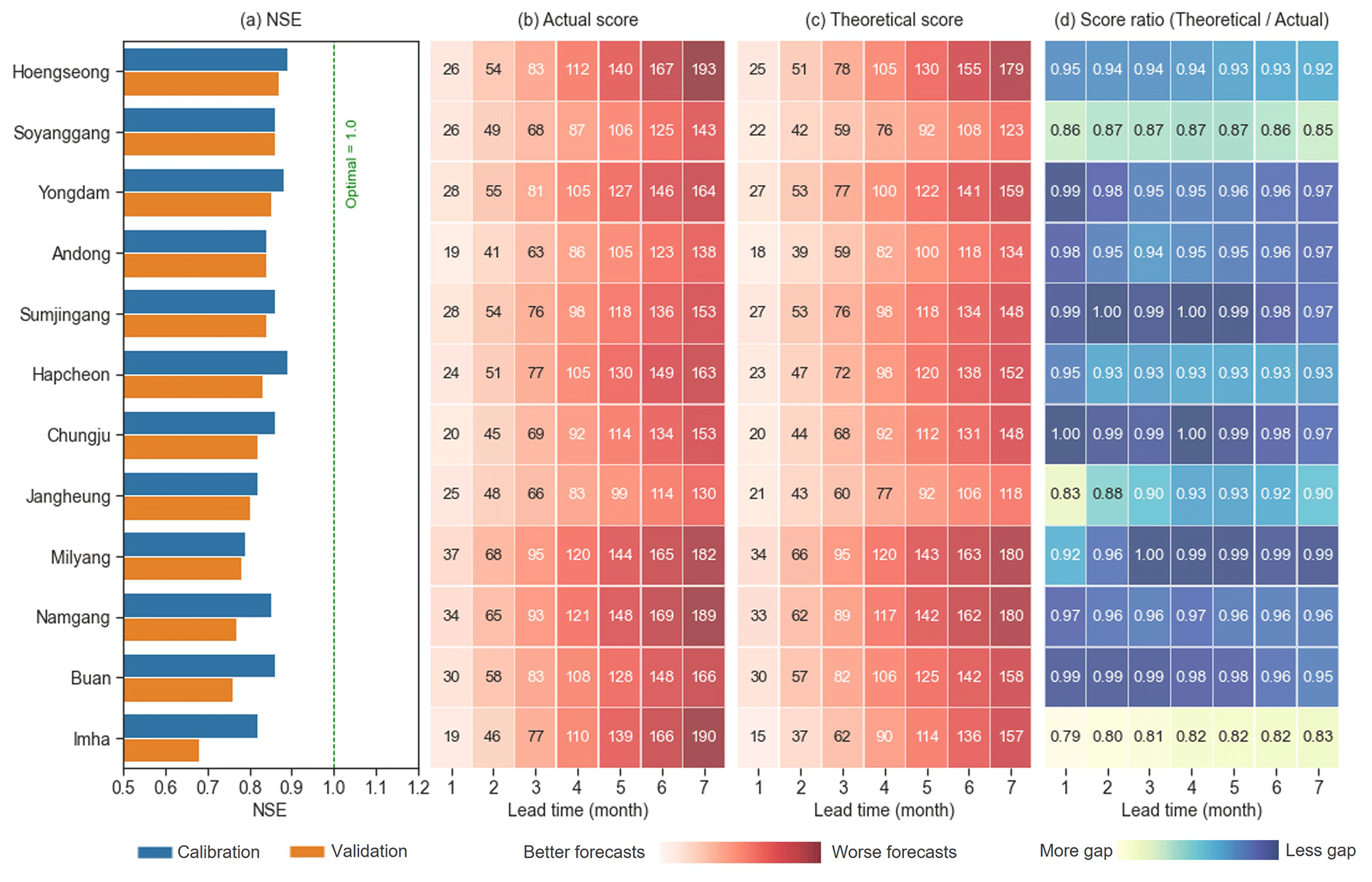
Figure 4 (a) Nash–Sutcliffe efficiency (NSE) of the hydrological models for the 12 catchments analysed in this study, (b) the actual score and (c) the theoretical score of SFFs, and (d) the score ratio (theoretical / actual) in terms of mean CRPS at different lead times (x axis) (the scores are calculated before the bias correction of weather forcings). The actual score is determined by comparing SFFs to flow observations. The theoretical score is determined by comparing SFFs to pseudo-observations produced by the same hydrological model forced by observed precipitation, temperature and PET.

Figure 4b and c represent the actual and theoretical scores (mean CRPS) over the period 2011–2020. Again, these are calculated by comparing the simulated flows with the observed flows (actual score) and with pseudo-observations (theoretical score), respectively. Since the CRPS is computed based on accumulated monthly flow at a given lead time, forecast errors also accumulate over time. Therefore, both scores considerably deteriorate as the lead time increases. Generally, the theoretical scores are slightly smaller than the actual scores, but the difference is marginal.

To facilitate comparison, the ratio between the actual score and the theoretical score is shown in Fig. 4d. For most catchments, the ratio values are close to 1, confirming the small gap between the actual and theoretical score. The noticeable exception is only seen in the Imha catchment, characterized by being the driest among the catchments and exhibiting the lowest modelling performance (Fig. 4a).

3.2 Contribution of weather forcings to the performance of SFFs

In this section, we quantify the contribution of each weather forcing forecast to the performance of SFFs, as measured by the CRPS (see Sect. 2.2 and Fig. S2 for details on the underpinning methodology). Figure 5 shows the relative scores for each non-bias-corrected weather forcing across all seasons (Fig. 5a), dry season (Fig. 5b) and wet season (Fig. 5c) at different lead times (1, 3 and 6 months). The relative score is calculated as the ratio of the integrated score (computed using seasonal weather forecasts for all weather forcings) to the isolated score (when SFFs are computed using seasonal forecasts for one weather forcing and observations for the other two). The closer the isolated score to the integrated score, the larger the contribution of that weather forcing to the overall performance (or lack of performance) of the SFFs.

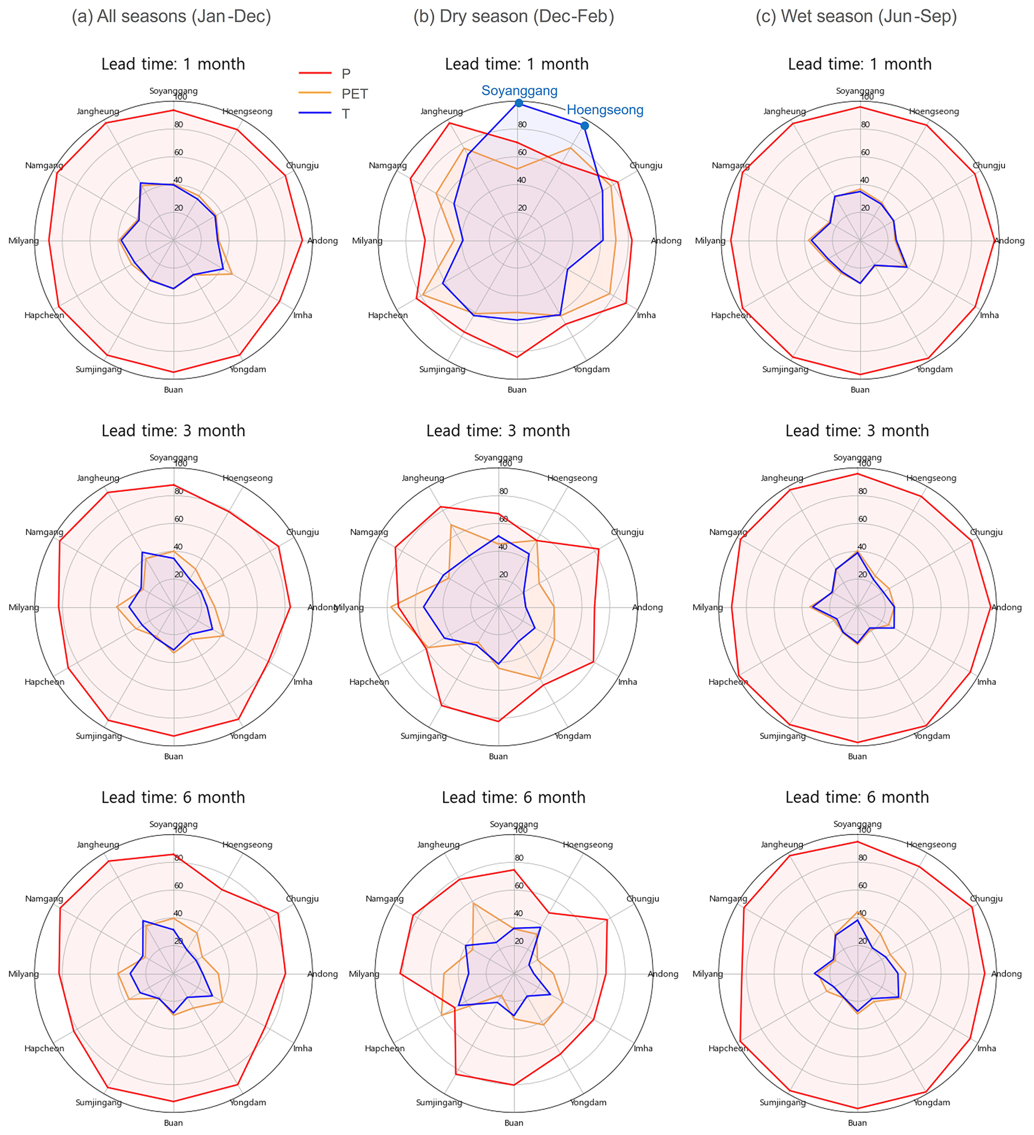
Figure 5 Relative score (in %) of each weather forcing (precipitation in red, PET in orange and temperature in blue) before bias correction compared to the score of SFFs averaged over 10 years (2011–2020) during (a) all seasons, (b) dry season and (c) wet season at 1, 3 and 6 lead months from top to bottom. Catchments are in order of their location, from the northernmost (Soyanggang) to the southernmost (Jangheung) one, in clockwise direction; see Fig. 1.

As shown in Fig. 5a, the contribution of each weather forcing to the performance of SFFs varies with catchment and lead time, but overall precipitation forecast plays a dominant role. Specifically, the contribution of the precipitation forecast (in red) accounts for almost 90 % of the integrated score, which is forced by seasonal weather forecasts for all weather forcings. Meanwhile, PET (in orange) and temperature (in blue) contribute a similar level, ranging between 30 % and 40 %.

During the dry season (Fig. 5b), however, PET and temperature show comparable levels of contribution to precipitation. This is more evident in the Soyanggang and Hoengseong catchments, which are both located in the northernmost region of South Korea (see Fig. 1). These catchments are characterized by low temperatures and heavy snowfall in the dry (winter) season. The correct prediction of temperature is thus crucial here as temperature controls the partitioning of precipitation into rain and snow and hence the generation of a fast or delayed flow response. Further analysis (shown in Fig. S4) reveals that temperature forecasts in these two catchments are consistently lower than those in the observation, which means that the hydrological model classifies rain as snow for several events, and hence retains that “snow” in the simulated snowpack, which in reality should produce a flow response. This explains the significant increase in performance when forcing the model with bias-corrected temperature instead (Fig. S4b).

In order to enhance the forecasting performance, we applied bias correction to each weather forcing and re-generated SFFs with bias-corrected weather forcings. In most catchments and lead times, the overall skill is improved after correcting biases. The overall skill increases by 46 % to 54 % on average across all seasons and more specifically from 31 % to 50 % in the dry season and from 54 % to 55 % in the wet season. The largest increase in overall skill is found in the Imha catchment, which has the lowest skill before correcting biases. For a detailed account of overall skill before and after bias correction, see Figs. S5 and S6.

Figure 6 illustrates the change in the relative score of each weather forcing after bias correction, focusing on the dry season and the first forecasting lead month. One notable finding is that, in the snow-affected catchments (Soyanggang and Hoengseong), there is a significant decrease in the relative score of temperature after applying bias correction. As shown in detail in Fig. S4, this is due to the correction of systematic underestimation biases in temperature forecasts, which leads to a more correct partitioning of precipitation into snow and rain and thus better flow predictions. The relative score of the forecasts for all seasons and lead times after bias correction is reported in Fig. S7.

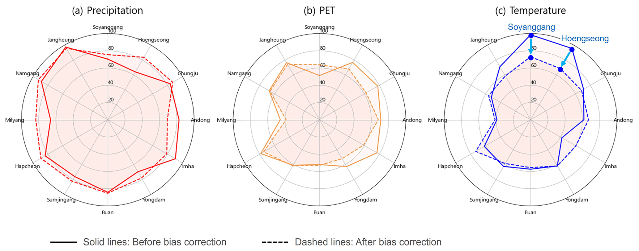
Figure 6 Relative score (in %) of each weather forcing – (a) precipitation, (b) PET and (c) temperature) – before (solid line) and after (dashed line) bias correction compared to the score of SFFs averaged over 10 years (2011–2020) during the dry season and first lead month.

3.3 Comparison between SFFs and ESP across seasons and catchments

In order to comprehensively compare the performance of SFFs and ESP, we employed the overall skill, which quantifies the frequency at which SFFs outperform ESP, as outlined in Sect. 2.2.3 (Eq.10). Figure 7 shows the seasonal and regional variations in overall skill (after bias correction) for all seasons (Fig. 7a), for the dry season (Fig. 7b) and for the wet season (Fig. 7c). For each catchment, the results are visualized as a table showing the overall skill at lead times of 1 to 6 months. The table cells are coloured in green (pink) when SFFs outperform ESP (ESP outperforms SFFs). Yellow colour indicates that the system and benchmark have equivalent performance. In principle, this happens when the overall skill is equal to 50 %; however, in order to avoid misinterpreting small differences in overall skill, we classified all cases as equivalent when the overall skill is between 45 % and 55 %. While the choice of the range (±5 %) is subjective, we find it helpful to assist analysis in avoiding spurious precision in a simple and intuitive manner.

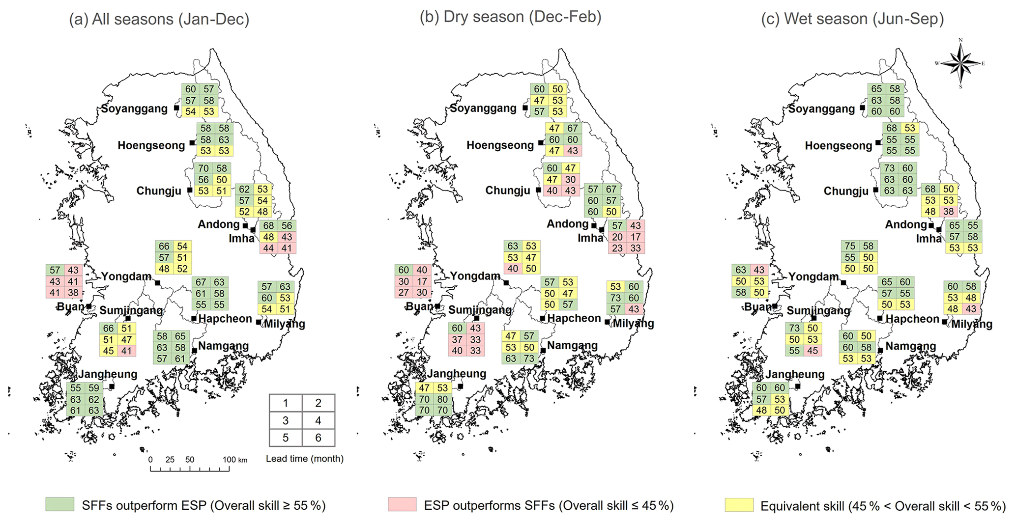
Figure 7 Map of the overall skill of bias-corrected SFFs for 10 years (2011–2020) over (a) all seasons, (b) dry season and (c) wet season. The colours represent whether SFFs outperform ESP or not for each catchment and lead time (1 to 6 months).

As shown in Fig. 7a, the overall skill of SFFs varies according to the lead time, season and catchment. SFFs generally outperform ESP, particularly up to 3 months ahead. At longer lead times, the results vary from catchment to catchment. For instance, in some catchments generally located in the southern region, such as Jangheung, Namgang and Hapcheon, SFFs outperform ESP for longer lead times. On the other hand, in some catchments, such as Imha and Buan, ESP generally exhibits a higher performance than SFFs. Specifically, two catchments, Buan, which is located in the western coastal region and has the smallest catchment area, and Imha, which is the driest catchment, show the lowest skill. Nevertheless, we could not identify a conclusive correlation between catchment characteristics such as size or mean annual precipitation and overall skill.

Comparing the results for the dry and wet seasons, Fig. 7b and c show that SFFs are much more likely to outperform ESP in the wet season, particularly in the catchments in the northernmost region. During the dry season, the overall skill of SFFs is lower, and particularly in the Buan, Imha and Sumjingang catchments, SFFs outperform ESP only for the first lead month.

3.4 Comparison between SFFs and ESP in dry and wet years

We now assess the influence of exceptionally dry and wet conditions on the overall skill of SFFs. Based on the mean annual precipitation across 12 catchments within the period 2011–2020, we classified the years 2015 and 2017 as dry (P<900 mm) and the years 2011 and 2020 as wet (P>1500 mm). Figure 8 shows the overall skill of SFFs averaged over 12 catchments for the entire period (Fig. 8a), dry years (Fig. 8b) and wet years (Fig. 8c) during all seasons (solid black line), dry season (dashed red line) and wet season (dashed blue line), respectively.

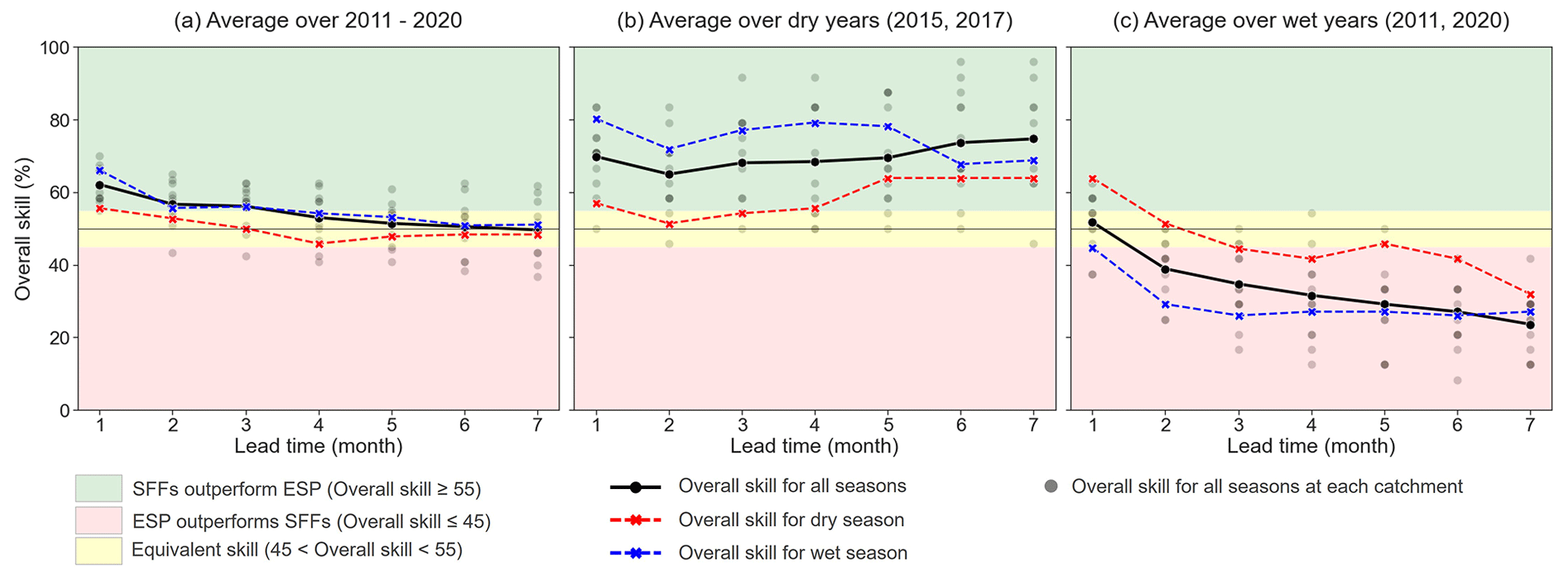
Figure 8 Overall skill of bias-corrected SFFs over 12 catchments averaged over (a) all years (2011 to 2020), (b) dry years (mean annual P<900 mm) and (c) wet years (mean annual P>1500 mm) during all seasons (black lines), dry seasons (dashed red lines) and wet seasons (dashed blue lines). The grey points represent the overall skill in each catchment. Here, mean annual precipitation is averaged across the catchments and years.

Figure 8a shows that SFFs generally outperform ESP for lead times of up to 3 months and maintain equivalent performance levels thereafter. In addition, it is evident that SFFs are more skilful during the wet season than during the dry season. In dry years (Fig. 8b), in contrast to the typical decrease in the overall skill with lead time, we find that SFFs maintain a significantly higher skill at all lead times, particularly during the wet season (blue line). On the other hand, during wet years (Fig. 8c), the overall skill is generally poor, and ESP generally has higher performance than SFFs, especially during the wet season.

Last, we analyse the spatial variability in the overall skill by looking at the spread of individual catchments (grey dots). We see that the spread in dry and wet years (Fig. 8b and c) is larger than in all years (Fig. 8a). This confirms that under extreme weather conditions, the uncertainty and variability in the forecasting performance increase depending on the catchment. A more detailed analysis of the overall skill for each catchment (described in Fig. S8) shows that the catchments located in the southern region consistently exhibit higher skill regardless of lead times and whether the years are dry/wet.

3.5 Example of flow forecasts time series

Figure 9 shows an example of the flow into the Chungju reservoir, which holds the largest storage capacity in South Korea. The overall skill of this catchment is the highest for a 1-month lead time; however, from the second lead month onward, it shows a moderate level of overall skill compared to other catchments (see Fig. S8). In this section, we compare the observed and forecasted cumulative flow forced by seasonal weather forecasts (SFFs; green lines) and historical weather records (ESP; pink lines) for lead times of 1, 3 and 6 months from April during the wettest (2011) and the driest year (2015), respectively.

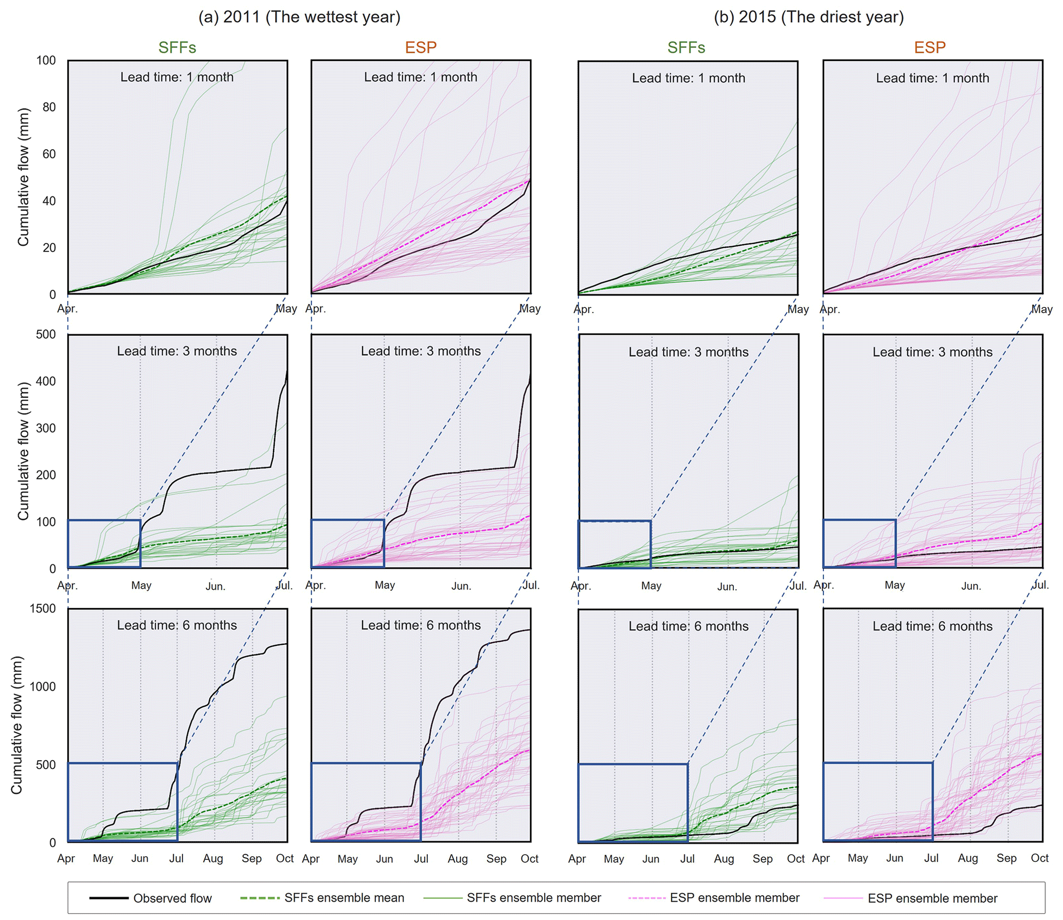
Figure 9 Observed cumulative flow (black lines) and forecasted cumulative flow representing SFFs after bias correction (green lines in left panels) and ESP (pink lines in right panels) in the Chungju reservoir for 1, 3 and 6 months of lead time over (a) the wettest year (2011; 1884 mm yr⁻¹) and (b) the driest year (2015; 74 mm yr⁻¹).

In this specific catchment and during these years, SFFs show equivalent or slightly higher performance than ESP at a 1-month lead time. However, as the lead time increases, the performance of both methods tends to deteriorate. Essentially, there is an underestimation in the wettest year (2011) and an overestimation in the driest year (2015) at the scale of the season. In particular, considerably higher performance was found in SFFs compared to ESP in the driest year (Fig. 9b). On the other hand, it is obvious that the performance of both methods is insufficient in forecasting flow in the wettest year for lead times of 3 and 6 months.

Examining each ensemble member of both SFFs and ESP, we found higher variability in ESP. Furthermore, since ESP utilizes the same weather forcings, the forecasted flows are generally similar in terms of its quantity and patterns regardless of the wettest and driest years. Conversely, the forecasted flow ensemble members of SFFs show distinctive patterns for each year.

Although these results are confined to a single catchment and specific years, this analysis is valuable in quantitatively illustrating the forecasted flow results under dry and wet conditions and different lead times. Furthermore, these features are generally shown in other catchments and align with our previous findings described in Sect. 3.4.

4 Discussion

4.1 The skill of seasonal flow forecasts

This study offers a comprehensive view of the overall skill of SFFs, benchmarked to the conventional – and easier to implement – ESP method. In contrast to the majority of previous studies, which assessed the skill of SFFs at the continental or national level or over large river basins, our study focuses on 12 relatively small catchments (59–6648 km²) across South Korea.

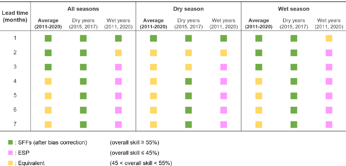
Table 2 summarizes the key findings of this study regarding the overall skill of SFFs across different seasons and years. It demonstrates that SFFs outperform ESP in almost all the cases for forecasting lead times of 1 month. This result is consistent with previous literature (e.g. Yossef et al., 2013; Lucatero et al., 2018). In addition, the higher skill of SFFs is also shown at lead times of 2 and 3 months in several situations, as shown in Table 2, and at even longer lead times in dry years. This is more surprising as this considerable performance of SFFs was not found in previous studies.

Table 2 Summary of key findings regarding the overall skill at different lead times, seasons and years.

Similarly to our study, earlier studies (Crochemore et al., 2016; Lucatero et al., 2018) have explored the skill compared with real flow observations at a catchment scale. Therefore, the comparison between their results and our findings holds interest. In brief, their results suggest that ESP remains a hard-to-beat method compared to SFFs even after bias correction. Crochemore et al. (2016) showed that SFFs using bias-corrected precipitation have an equivalent level of performance with ESP up to 3 months ahead. Lucatero et al. (2018) concluded that SFFs still face difficulties in outperforming ESP, particularly at lead times longer than 1 month.

The difference in our results compared to the literature stems from a combination of several important factors. First, it is worth noting that these two previous studies were conducted at the catchment scale, with a specific focus on Europe – namely France (Crochemore et al., 2016) and Denmark (Lucatero et al., 2018). The skill of SFFs varies according to the geographical locations and meteorological conditions in a given study area, as confirmed by numerous studies (e.g. Yossef et al., 2013; Greuell et al., 2018; Pechlivanidis et al., 2020). Therefore, the skill of SFFs could also be influenced by distinct spatial and meteorological conditions between Europe and South Korea.

Second, we can attribute the difference to the utilization of a more advanced seasonal weather forecasting system. Unlike previous studies which applied ECMWF System 4, our study is conducted based on version 5 of ECMWF's cutting-edge forecasting system. It is reported that ECMWF SEAS5 has improved significantly compared to the previous version, including the predictive skill of the El Niño–Southern Oscillation (ENSO) (Johnson et al., 2019) and rainfall inter-annual variability (Köhn-Reich and Bürger, 2019). Specifically, ENSO is known to be a key driver affecting the skill of seasonal weather forecasts (Weisheimer and Palmer, 2014; Shirvani and Landman, 2015; Ferreira et al., 2022); therefore, its improvement can result in notable changes in forecasting skill. Although the relationship between seasonal weather patterns in South Korea and ENSO is not fully understood, some previous research has shown good correlations in certain regions and seasons (Lee and Julien, 2016; Noh and Ahn, 2022). In this study, it is challenging to quantitatively evaluate the impact of system advancements. However, given the significance of meteorological forecasts in hydrological forecasts, it is highly probable that the development of the system has had a positive influence on the results. Although a few studies have analysed the skill of SFFs based on ECMWF SEAS5 (e.g. Peñuela et al., 2020; Ratri et al., 2023), direct comparisons with our research were deemed difficult due to differences in spatial scale and analysis methods, such as the absence of a comparison with ESP.

Lastly, the performance of the hydrological model also contributes to differences in the results. To evaluate the impact of the hydrological model on SFFs, we compared the actual score (forecast performance compared to observed flow data) with the theoretical score (forecast performance compared to pseudo flow observations) and found that the actual scores are slightly higher than theoretical scores (i.e. theoretical scores show a higher performance). This finding is consistent with previous studies, and the gap between the actual and theoretical score is highly linked to the performance of the hydrological model (Van Dijk et al., 2013; Greuell et al., 2018). When a model's actual score closely approximates its theoretical score, it may suggest that the model is operating at the best possible level given the inherent uncertainties and limitations associated with the available data and methods. Although our results demonstrated that the theoretical score shows higher performance than the actual score, their difference was generally marginal. This close agreement between the two scores indicates that the model is well calibrated and capable of effectively capturing the underlying hydrological processes in those catchments.

Our findings on the impact of bias correction quantitatively showed that generally precipitation controls the performance of SFFs; however, we also found that temperature plays a substantial role in specific seasons and catchments. Specifically, the Hoengseong and Soyanggang catchments, located in the northernmost part of South Korea and affected by snowfall in the dry (winter) season (December to February), exhibit a higher temperature contribution than precipitation for a forecasting lead time of 1 month during the dry season. The main reason for this is the underestimation of temperature forecasts. Our supplementary experiments provide evidence that using bias-corrected temperature forecasts significantly improves the performance of flow forecasts (see Fig. S4). Although the positive impact of bias correction of precipitation forecasts on enhancing the performance of SFFs has been well documented in numerous previous studies (Crochemore et al., 2016; Lucatero et al., 2018; Tian et al., 2018; Pechlivanidis et al., 2020), our result demonstrates the importance of bias correction of temperature too, at least in snow-affected catchments.

An alternative approach to bias correction has been proposed by Yuan and Wood (2012) and Lucatero et al. (2018), who argue that directly correcting the biases in the flow forecasts may result in a better performance at a lower computational cost. However, we tested this approach and found conflicting outcomes (Fig. S9). Therefore, caution should be exercised when directly correcting biases for flow as this approach may exclude the contribution of initial conditions, which is one of the most crucial factors in hydrological modelling. In the cases where the performance of hydrological model is the major source of error, bias correction of the flow might be useful; however, if the model shows an acceptable performance, as demonstrated in this study, incorporating bias correction into the simulated flow could add more errors.

Due to limited data availability, conducting additional validation across a larger number of extreme events is not possible. Nevertheless, our research findings suggest a potential correlation between the overall skill and dry/wet conditions, which should be further validated if new data become available. Specifically, in the period analysed here, SFFs considerably outperform ESP for all lead times during the wet season in dry years. Conversely, the overall skill during the wet season in wet years was not satisfactory. This is because the overall skill is commonly dominated by precipitation forecasting skill, and we previously found that the skill of precipitation forecasts is the lowest in wet years (Lee et al., 2023). The systematic biases of seasonal precipitation forecasts, which tend to underestimate (overestimate) the precipitation during the wet (dry) season, led to the consistent results in flow forecasts. This finding also hints at the fact that SFFs hold the potential to provide valuable information for effective water resources management during dry conditions, which is crucial for drought management.

4.2 Limitations and directions for future research

In this paper, we investigated the overall skill of SFFs at the catchment scale using ECMWF's seasonal weather forecasts (SEAS5) with a spatial resolution of 1°×1°. Based on our previous research, it has been demonstrated that among four forecasting centres, ECMWF provides the most skilful seasonal precipitation forecasts (Lee et al., 2023); thus, we utilized seasonal weather forecast datasets from ECMWF in this study. However, the skill to forecast other weather forcings, such as temperature and PET, has not been tested across South Korea. Additionally, while ECMWF originally generates seasonal weather forecasts with high resolution (36×36 km, which is approximately 0.3°×0.3°), we utilized publicly available low-resolution data (1°×1°) provided by CCDS to maintain consistency with our previous work (Lee et al., 2023). Our additional investigation indicates that the difference in weather data between high and low resolutions is not substantial (see Fig. S10). Nevertheless, prior studies suggest that the skill of seasonal weather forecasts may vary according to factors such as region, season and spatial resolution. Therefore, broader research is required to determine the seasonal weather forecasts provider as well as spatial resolution that can lead to skilful hydrological forecasts in the regions or seasons of interest.

Given the distinct climatic conditions in South Korea, it is important to acknowledge that our results may not be applicable to other regions or countries. Therefore, further work needs to be carried out to reproduce this analysis in different regions. To facilitate this process, two Python-based toolboxes can be useful: SEAFORM (SEAsonal FORecasts Management) and SEAFLOW (SEAsonal FLOW forecasts). The SEAFORM toolbox, developed in our previous study (Lee et al., 2023), offers multiple functions for manipulating seasonal weather forecast datasets (e.g. downloading the datasets, generating the time series and correcting the bias). On the other hand, the SEAFLOW toolbox, developed in this study, is specifically designed for the analysis of SFFs based on the modified Tank model (but it could be useful to apply it to other hydrological models).

In terms of forecast skill, our study highlights the potential of SFFs at the catchment scale for real water resources management. Nevertheless, it is crucial to recognize the difference between skill, which indicates how well hydrological forecasts mimic observed data, and value, which refers to the practical benefits obtained by utilizing those forecasts in the real world. Previous studies have addressed this issue, showing that better skill does not always result in higher value (Chiew et al., 2003; Boucher et al., 2012). While earlier findings suggest that the conventional method (ESP) generally outperforms SFFs in terms of skill (e.g. Yossef et al., 2013; Lucatero et al., 2018), recent research demonstrates that, in terms of value, the use of seasonal forecasts in semi-arid regions offers significant economic benefits by mitigating hydropower losses in a dry year (Portele et al., 2021). Therefore, our future research efforts should concentrate on a quantitative evaluation of the value of SFFs for practical reservoir operations, informing decision-making in water resources management. This evaluation is of significant importance as it directly relates to assessing the potential utilization of SFFs in practical water management.

5 Conclusions

This study assessed the overall skill of SFFs across 12 catchments in South Korea using a hydrological model forced by seasonal weather forecasts from ECMWF (SEAS5). By focusing on operational reservoir catchments with relatively small sizes, our findings showed the potential of SFFs in practical water resources management.

The results first demonstrate that the performance of the hydrological model is crucial in flow forecasting, with the Tank model used in this study exhibiting reliable performance. Secondly, precipitation emerges as a dominant factor influencing the performance of SFFs compared to other weather forcings, and this is more evident during the wet season. However, temperature can also be highly important in specific seasons and catchments, and this result highlights the significance of temperature bias correction as the flow simulation with the bias-corrected temperature provides higher performance. Third, at the catchment scale, which is more suitable for water resources management, bias-corrected SFFs have skill with respect to ESP up to 3 months ahead. Notably, the highest overall skill during the wet season in dry years highlights the potential of SFFs to add value in drought management. Lastly, while our research emphasizes the superior performance of SFFs at the catchment scale in South Korea, it is important to note that outcomes may vary depending on factors such as the type of seasonal weather forecast system used, the study area and the performance of the hydrological model.

As seasonal weather forecasting technologies continue to progress, it is also crucial to concurrently pursue their application and validation in flow forecasting. We hope that our findings contribute to the ongoing validation efforts of the skill of SFFs across various regions and, furthermore, serve as a catalyst for their practical application in real-world water management. At the same time, our proposed workflow and the analysis package we have developed using a Python Jupyter Notebook can offer valuable support to water managers in gaining practical experience so that they could utilize SFFs more effectively.