the Creative Commons Attribution 4.0 License.
the Creative Commons Attribution 4.0 License.
 | 23 Jul 2024
Scientific logic and spatio-temporal dependence in analyzing extreme-precipitation frequency: negligible or neglected?
Francesco Serinaldi
Statistics is often misused in hydro-climatology, thus causing research to get stuck on unscientific concepts that hinder scientific advances. In particular, neglecting the scientific rationale of statistical inference results in logical and operational fallacies that prevent the discernment of facts, assumptions, and models, thus leading to systematic misinterpretations of the output of data analysis. This study discusses how epistemological principles are not just philosophical concepts but also have very practical effects. To this aim, we focus on the iterated underestimation and misinterpretation of the role of spatio-temporal dependence in statistical analysis of hydro-climatic processes by analyzing the occurrence process of extreme precipitation (P) derived from 100-year daily time series recorded at 1106 worldwide gauges of the Global Historical Climatology Network. The analysis contrasts a model-based approach that is compliant with the well-devised but often neglected logic of statistical inference and a widespread but theoretically problematic test-based approach relying on statistical hypothesis tests applied to unrepeatable hydro-climatic records. The model-based approach highlights the actual impact of spatio-temporal dependence and a finite sample size on statistical inference, resulting in over-dispersed marginal distributions and biased estimates of dependence properties, such as autocorrelation and power spectrum density. These issues also affect the outcome and interpretation of statistical tests for trend detection. Overall, the model-based approach results in a theoretically coherent modeling framework where stationary stochastic processes incorporating the empirical spatio-temporal correlation and its effects provide a faithful description of the occurrence process of extreme P at various spatio-temporal scales. On the other hand, the test-based approach leads to theoretically unsubstantiated results and interpretations, along with logically contradictory conclusions such as the simultaneous equi-dispersion and over-dispersion of extreme P. Therefore, accounting for the effect of dependence in the analysis of the frequency of extreme P has a huge impact that cannot be ignored, and, more importantly, any data analysis can be scientifically meaningful only if it considers the epistemological principles of statistical inference such as the asymmetry between confirmatory and disconfirmatory empiricism, the inverse-probability problem affecting statistical tests, and the difference between assumptions and models.
- Article
(10072 KB) - Full-text XML
-
Supplement
(1898 KB) - BibTeX
- EndNote


1.1 Epistemology of scientific inquiry: “model-based” data analysis
Most of the methods reported in handbooks of applied statistics have been developed under the assumption of independence, distributional identity and stationarity, and well-behaving bell-shaped or exponential distributions. Of course, there is a wide array of statistical literature focused on dependence and the related stochastic processes, the lack of distributional identity and nonstationarity, and skewed sub-exponential distributions. However, in some applied sciences such as hydro-climatology, analysts have often neglected the fact that moving from the former set of assumptions (commonly reported in introductory handbooks) to the latter is not just moving to a more general model from one that can be considered to be a special case. A typical example is the generalized extreme value (GEV) distribution, widely used in the study of hydro-climatic extreme events, which converges to the Gumbel distribution as the shape parameter converges to zero. While Gumbel is mathematically a special case of the GEV, assuming that Gumbel is the distribution of choice has relevant consequences as it means assuming exponential tails instead of super-exponential (upper-bounded) or sub-exponential (possibly heavy) tails. In particular, high values of skewness and heavy tails imply possible non-existence of the moments of high order, as well as bias and/or high variability in the estimates of the moments themselves, including variance, covariance, and autocorrelation, as well as long-range dependence (see, e.g., Embrechts et al., 2002; Barunik and Kristoufek, 2010; Lombardo et al., 2014; Cirillo and Taleb, 2016; Taleb, 2020; Dimitriadis et al., 2021; Koutsoyiannis, 2023, and references therein).
Similar remarks hold for nonstationarity, which denotes the dependence of the (joint) distribution function of a set of generic random variables Xt on the parameter t () via well-specified functions of t (e.g., Koutsoyiannis and Montanari, 2015; Serinaldi et al., 2018). For example, if t denotes “time”, dealing with nonstationarity does not mean just adding time-dependent parameters to a stationary model using, for instance, generalized linear models (GMLs) and their available extensions; it means that the ergodicity property, which is key in the interpretation of statistical inference, is no longer valid (e.g., Koutsoyiannis and Montanari, 2015). In these cases, any estimate of whatever summary statistics, such as the sample mean, is uninformative as it does not have a corresponding unique population counterpart since the latter does not exist anymore (e.g., Serinaldi and Kilsby, 2015).
As for the effects of nonstationarity and heavy tails, there is a wide array of literature on the effects of the assumption of dependence on statistical inference. Generally, dependence implies information redundancy and a reduced effective sample size, along with variance inflation and bias in the standard estimators of summary statistics such as marginal and joint moments (e.g., Koutsoyiannis, 2004; Lombardo et al., 2014; Dimitriadis and Koutsoyiannis, 2015, and references therein). Therefore, assuming spatio-temporal dependence means recognizing that such an assumption impacts every sampling property of the process, including marginal distributions. Under spatio-temporal dependence, the classical estimator of the correlation itself is biased and needs to be corrected (e.g., Marriott and Pope, 1954; White, 1961; Wallis and O'Connell, 1972; Lenton and Schaake, 1973; Mudelsee, 2001; Koutsoyiannis, 2003, 2011; Koutsoyiannis and Montanari, 2007; Papalexiou et al., 2010; Tyralis and Koutsoyiannis, 2011; Dimitriadis and Koutsoyiannis, 2015; Serinaldi and Kilsby, 2016a).
The foregoing examples highlight that the statistical inference cannot be reduced to the usage of multiple competing models and methods as every aspect of statistical analysis and its interpretation depends on the underlying assumptions according to the rationale of statistical inference. Even the simplest diagnostic diagram relies on underlying assumptions and models (see, e.g., Serinaldi et al., 2020a, for further discussion). This primary epistemological concept comes before any methodology and/or technicality and marks the boundary between correct interpretation and misinterpretation of inference results and, eventually, “between engineering concepts dictated by expediency, and scientific truth” (Klemeš, 1986). However, while this was routinely presented in statistical handbooks published in the past century (e.g., Aitken, 1947; Cramér, 1946; Papoulis, 1991), most of the modern textbooks seem to miss it, perhaps taking it for granted. Nonetheless, in the hydro-climatological context, von Storch and Zwiers (2003, p. 69) summarized well the primary principles of statistical inference as follows:
-
“A statistical model is adopted that supposedly describes both the stochastic characteristics of the observed process and the properties of the method of observation. It is important to be aware of the models implicit in the chosen statistical method and the constraints those models necessarily impose on the extraction and interpretation of information.”
-
“The observations are analysed in the context of the adopted statistical model.”
These concepts are nothing but the specialization of the principles of scientific inquiry in the context of data analysis. As stressed by Box (1976), “science is a means whereby learning is achieved, not by mere theoretical speculation on the one hand, nor by the undirected accumulation of practical facts on the other, but rather by a motivated iteration between theory and practice... Matters of fact can lead to a tentative theory. Deductions from this tentative theory may be found to be discrepant with certain known or specially acquired facts. These discrepancies can then induce a modified, or in some cases a different, theory. Deductions made from the modified theory now may or may not be in conflict with fact, and so on”. Eventually, “the sciences do not try to explain, they hardly even try to interpret, they mainly make models. By a model is meant a mathematical construct which, with the addition of certain verbal interpretations, describes observed phenomena. The justification of such a mathematical construct is solely and precisely that it is expected to work – that is, correctly to describe phenomena from a reasonably wide area. Furthermore, it must satisfy certain esthetic criteria – that is, in relation to how much it describes, it must be rather simple” (von Neumann, 1955).
Based on the foregoing remarks, appropriate statistical inference (and scientific learning) is an iterative “model-based” procedure, which can be summarized as follows:
-
Make assumptions that are deemed to be reasonable for the data and facts at hand.
-
Build tentative theories and models and make inferences accounting for the effect and consequences of the underlying assumptions.
-
Interpret results according to the nature of the adopted assumptions and models.
-
Retain or change/update assumptions and models based on the agreement or disagreement of the developed theories and models with (new) data and facts.
This procedure should be iterated bearing in mind that the developed models should satisfy some formal criteria such as parsimony, accuracy, generality, and being fit for purpose.
1.2 Box's cookbookery and mathematistry: “test-based” data analysis
Being the prerequisite to any sound scientific investigation, the epistemological principles described in Sect. 1.1 should be obvious and well-known. However, this does not seem to be the case in some applied sciences where data analysis and modeling often neglect or ignore such principles, thus calling into question the scientific validity of results and conclusions.
In this respect, the statistician George E. P. Box highlighted that scientific progress results from the feedback between theory and practice, and this feedback requires a closed loop. Therefore, when the loop is open, progress stops. Box (1976) referred to the main consequences of a lack of feedback between theory and practice as maladies called “cookbookery” and “mathematistry”, claiming that “The symptoms of the former are a tendency to force all problems into the molds of one or two routine techniques, insufficient thought being given to the real objectives of the investigation or to the relevance of the assumptions implied by the imposed method… Mathematistry is characterized by development of theory for theory's sake, which since it seldom touches down with practice, has a tendency to redefine the problem rather than solve it… In such areas as sociology, psychology, education, and even, I sadly say, engineering, investigators who are not themselves statisticians sometimes take mathematistry seriously. Overawed by what they do not understand, they mistakenly distrust their own common sense and adopt inappropriate procedures devised by mathematicians with no scientific experience”.
In the context of climate science, von Storch and Zwiers (2003) raised similar remarks in the preface of their book: “Cookbook recipes for a variety of standard statistical situations are not offered by this book because they are dangerous for anyone who does not understand the basic concepts of statistics”.
This problem is not new in hydrology and hydro-climatology either and was already stressed by Yevjevich (1968) and Klemeš (1986), who discussed some misconceptions concerning the study and interpretation of hydrological processes and variables by methods borrowed from other disciplines such as systems and decision theory, mathematics, and statistics. For instance, often, stochastic processes are no longer considered to be convenient descriptors of hydrological processes for practical purposes, but the former are identified with the latter and vice versa, thus generating confusion and a questionable approach to data analysis and modeling that contrasts with the logic of statistical inference recalled in Sect. 1.1.
A large body of the literature on data analysis of unrepeatable hydro-climatic processes seems to neglect or ignore epistemological principles, thus confusing the role of observations, assumptions, and models. This results in fallacious procedures that share the following general structure, which we call the “test-based” method:
-
Select several models and methods based on different and often incompatible assumptions.
-
Make inferences neglecting the constraints imposed by different underlying assumptions.
-
Interpret results attempting to prove or disprove models' assumptions, which are often (if not always) erroneously attributed to physical processes, whereas they refer to models used to describe such processes.
This approach generally corresponds to a widespread mechanistic use of statistical methods or software and a massive application of statistical hypothesis tests, which are not supported by the required epistemological and theoretical knowledge of the methodologies used. Such an approach neglects the fact that models cannot be used to prove or disprove their own assumptions in the same way a mathematical theory cannot prove or disprove its own axioms and definitions. This is because those models and theories are valid only under those assumptions, axioms, and definitions. Of course, specific models cannot even be used to prove or disprove alternative assumptions as they might not even exist under those alternative hypotheses.
1.3 Aims and organization of this study
While Yevjevich (1968) and Klemeš (1986) provided extemporaneous commentaries about the foregoing issues, we address the problem from a different perspective. Instead of discussing several misconceptions from a general and purely conceptual point of view, we focus on a specific issue (here, the role of dependence in the statistical analysis of the occurrence of extreme precipitation (P)), focusing on theoretical inconsistencies and showing practical consequences by performing a detailed data analysis. In this way, theoretical remarks are complemented by a side-by-side comparison of the output of model-based and test-based methods, emphasizing the concrete effect of conceptual mistakes. Therefore, this work is a proper neutral validation and/or falsification study (see, e.g., Popper, 1959; Boulesteix et al., 2018, and references therein) that expands upon some of the existing literature about the independent check of the theoretical consistency in statistical methods applied in hydro-climatology (Lombardo et al., 2012, 2014, 2017, 2019; Serinaldi and Kilsby, 2016a; Serinaldi et al., 2015, 2018, 2020a, b, 2022).
Focusing on the assumption of spatio-temporal dependence in the analysis of extreme-P frequency, we attempt to show the practical consequences of underestimating and not properly considering and interpreting the effects of dependence, as well as the logical fallacies of the test-based method in this context. In particular, we re-analyze a worldwide precipitation data set comparing the output of a model-based framework (relying on theoretically informed stochastic modeling and diagnostic plots) with that of a test-based approach that led Farris et al. (2021) to conclude that “accounting or not for the possible presence of serial correlation has a very limited impact on the assessment of trend significance in the context of the model and range of autocorrelations considered here” and “Accounting for serial correlation in observed extreme precipitation frequency has limited impact on statistical trend analyses”. Therefore, this study double-checks the role of scientific logic and spatio-temporal dependence in the analysis and characterization of extreme-P frequency at various spatio-temporal scales. Eventually, we compare the two methodologies (model-based and test-based) in terms of their rationale and output to better understand why and how epistemological fallacies and the consequent improper use of statistical analysis and the treatment of dependence might result in misleading conclusions.
This study is organized according to its specific purpose. Therefore, it does not follow the standard structure of problem–model–application–results. In particular, all technical details of models and methods are reported in the Supplement. Indeed, the aim is to emphasize the practical importance of epistemology in data analysis rather than to focus on models' technicalities, which is one of the conceptual mistakes affecting test-based analysis. In this respect, the specific models and methods used are secondary and replaceable with others, whereas the logical reasoning leading the analysis (but systematically neglected in the test-based approach) stays unchanged.
Based on the foregoing remarks, Sect. 2 introduces the P data set. Section 3 presents and discusses the test-based methodology, highlighting shortcomings and pitfalls that lead us to introduce the rationale of a model-based approach, which is described in Sect. 4. In Sect. 5, we analyze the P frequency data, focusing on (i) the marginal distribution of the annual number (Z) of over-threshold (OT) events, (ii) the relationship between the lag-1 autocorrelation ρ1 and the slope ϕ of linear trends estimated based on the Z time series, and (iii) trend analysis of the Z time series. In this respect, we expand the analysis reported by Farris et al. (2021) by focusing on the role of spatio-temporal dependence at various spatio-temporal scales (e.g., Koutsoyiannis, 2020; Dimitriadis et al., 2021). For each stage of the foregoing analysis, we further discuss the logical consistency or pitfalls of the used methodologies and provide empirical results. Finally, Sect. 6 provides general remarks about the interpretation of our study in the context of the existing literature on statistical trend analysis and, more generally, about the problem of approaching the statistical analysis of hydro-climatic data while neglecting epistemological principles that are fundamental to properly set up the analysis itself.
We analyze daily precipitation time series from a sub-set of gauges extracted from more than 100,000 stations of the Global Historical Climatology Network-Daily (GHCN-D) database (Menne et al., 2012a, b) (https://www.ncei.noaa.gov/data/global-historical-climatology-network-daily/, last access: 17 February 2023). To allow a fair comparison with the existing literature, we extracted 1106 worldwide gauges characterized by at least 95 complete years of records in a common 100-year period from 1916 to 2015, using the same criteria applied by Farris et al. (2021). Figure 1 displays the map of the selected GHCN stations, with four sub-regions denoted as North America, Eurasia, Australia, and northwestern Europe. The first three regions are identified to be as close as possible to those used by Farris et al. (2021) in their regional analysis, while northwestern Europe is an additional region corresponding to the most densely gauged area of Eurasia. Overall, the four regions, along with the worldwide scale (hereinafter denoted as “world”), allow us to highlight the behavior of extreme P in nested regions.
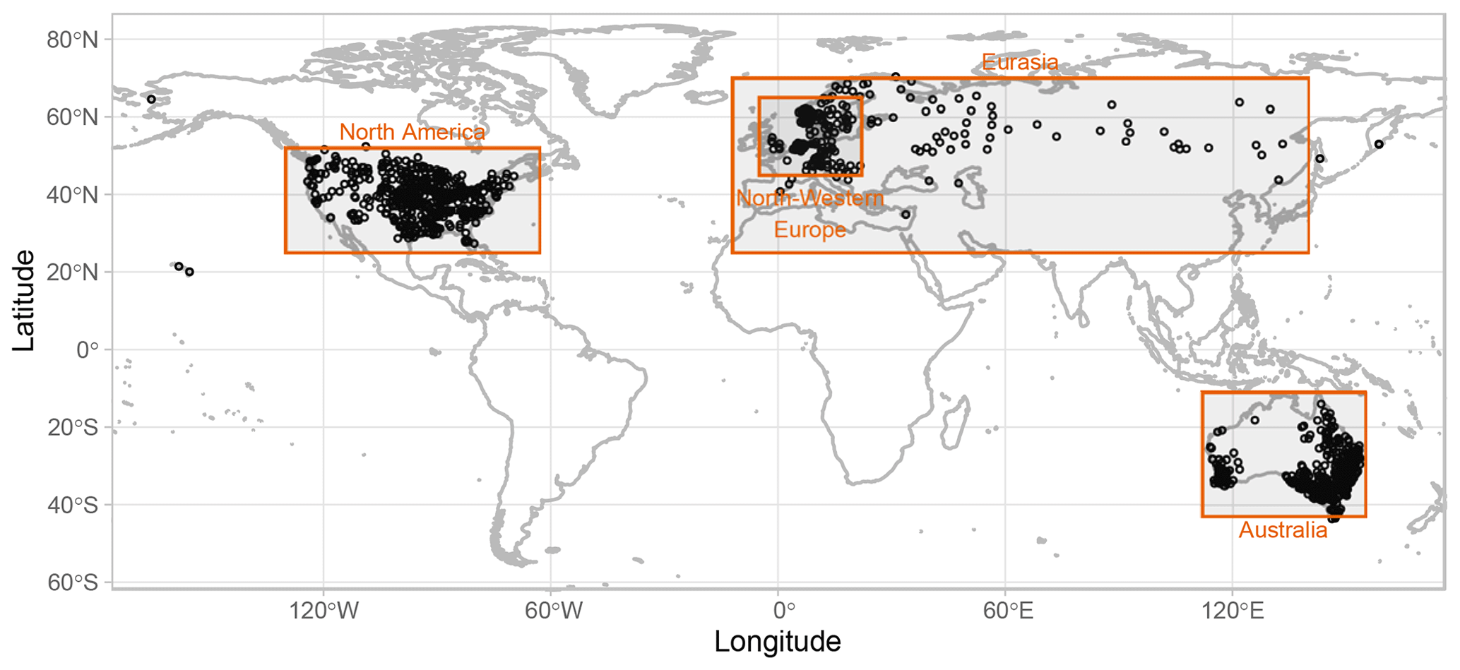
Figure 1Map of GHCN rain gauges used in this study, with the four sub-regions (denoted as North America, Eurasia, northwestern Europe, and Australia) that are discussed in the subsequent analysis.
To allow a fair comparison with the existing literature, we followed Farris et al. (2021) and selected extreme P to be the values exceeding given percentage thresholds according to the at-site empirical cumulative distribution function (ECDF) (including zeros). For each station, the annual number Z of OT exceedances forms the time series of extreme-P frequencies. Note that the “exceedances on consecutive days are counted as separate events” (Farris et al., 2021). Farris et al. (2021) considered several percentage threshold from 90 % to 97.5 % and different sub-sets (i.e., the most recent 30 and 50 years, as well as the complete sequences of 100 years). Since their results are consistent across different thresholds, we limit our analysis to the 95 % and 99.5 % thresholds as the former is the one discussed more extensively by Farris et al. (2021), while the latter serves to highlight the behavior of the occurrence process of P exceedances over a high threshold. As far as the number of years is of concern, we only use 100 and 50 years as shorter time series of 30 annual data points do not provide reliable information on occurrence processes in terms of spatio-temporal properties. The GHCN-D data set was retrieved and handled by the R-contributed package rnoaa (Chamberlain, 2020).
3.1 Assumptions and statistical tests
Before introducing the model-based methodology, we firstly present the test-based approach to data analysis. The aim is two-fold: (i) to explain the motivation of moving from test-based to model-based analysis and (ii) to better understand the discussion in Sect. 5 concerning the differences between the outputs of the two methodologies. For the sake of comparison, we apply the same test-based procedure used by Farris et al. (2021). It consists of the following steps:
-
Firstly, Kolmogorov–Smirnov (KS) and χ2 goodness-of-fit tests are used to check whether Z follow a Poisson distribution.
-
Based on the outcome of the first step, two competing models are selected: (i) the non-homogeneous Poisson (NHP) process describing a collection of independent Poisson random variables, with the rate of occurrence linearly varying with time, and (ii) the first-order Poisson integer autoregressive (Poisson-INAR(1)) process, which is a specific kind of stationary and temporally correlated process with a Poisson marginal distribution (see Sect. S1 in the Supplement). These models are used to study the effect of serial correlation.
-
Therefore, various statistical tests for trend detection are applied. Due to similar performance of parametric and nonparametric tests, Farris et al. (2021) retained and discussed only one test for each category, that is, a nonparametric test based on the Mann–Kendall (MK) test statistic and a parametric test based on the slope parameter of a Poisson regression (PR).
Incidentally, when performing a statistical test at the α significance level many times, we expect a percentage α of false rejections on average. Since all tests are applied to multiple time series, the false-discovery rate (FDR) method – that is, the ratio of the number of false rejections to all rejections (Benjamini and Hochberg, 1995) – is used to account for the effect of test multiplicity, which is also known as field significance (Wilks, 2016; Farris et al., 2021).
The aim of this trend analysis of Z is to investigate the impact of serial correlation on trend detection and the effect of performing multiple tests. Even though technicalities (such as the selection of a particular test or model) can change from case to case, it is easy to recognize that the foregoing procedure follows the same test-based rationale of trend analyses reported in the majority of the literature on this topic. However, are we sure that such a way of analyzing data is compliant with the scientific method and its logic? Can we consider test-based analysis to be theoretically consistent solely due to its widespread application? In the next section, we start to answer these questions.
3.2 Remarks on logical fallacies of the test-based methodology
As mentioned in Sect. 1, every statistical analysis (including diagnostic plots) relies on some assumptions, and these assumptions lead the interpretation of results. In this respect, while the simultaneous application of the techniques or tests listed in the previous section seems to be reasonable, a closer look reveals that the assumptions behind these statistical methods are not compatible with each other and might yield logical contradictions.
For example, KS and χ2 goodness-of-fit tests, which are used to check the suitability of the Poisson distribution for Z, are valid under the assumption that the underlying process is independent and identically distributed. Therefore, if these tests pointed to a lack of rejection of Poisson distributions, this would also imply independence and distributional identity (i.e., stationarity). In fact, if the process were not independent, dependence would generate information redundancy and over-dispersion (variance larger than the mean) of the observed finite-size samples of Z, thus making the Poisson model unsuitable from a theoretical standpoint. On the other hand, if the Z process were time-nonstationary (i.e., not identically distributed), we could not conclude that the distribution of Z is a single, specific distribution, such as Poisson. In that case, the distribution of Z can be, at most, conditionally Poisson (i.e., a Poisson distribution describes the process resulting from filtering nonstationarity out) or compound Poisson (i.e., a compound Poisson distribution describes the process resulting from incorporating nonstationarity by model averaging over time). Therefore, if the Poisson assumption is not rejected according to tests that imply independence and stationarity, we must necessarily exclude the alternative assumptions of dependence and nonstationarity, thus concluding that there is no reason to further proceed with any subsequent analysis of trends and/or dependence. This is the first logical contradiction of the test-based procedure described in Sect. 3.1.
Nonetheless, let us overlook the foregoing contradiction and move to the second step of the procedure. If we assume that the Z process is NHP, this model implies that the data follow a different Poisson distribution at each time step (see Sect. S1 in the Supplement). In this case, the overall distribution of the observed Z is a compound Poisson, and, more importantly, the nonstationarity of NHP hinders the application of KS and χ2 goodness-of-fit tests as the process does not fulfill the underlying assumptions of these tests. Indeed, these tests can, at most, be applied to conditional processes – that is, to values resulting from filtering the effect of “non-homogeneity” out (see e.g., Coles, 2001, p. 110–111). In the present case, non-homogeneity can consist of random fluctuations or a well-defined evolution of the rate of occurrence of extreme P. To summarize, if we assume NHP (and therefore nonstationarity), the results of the first step are theoretically invalid, and they should be discarded a priori. This is the second logical contradiction of the test-based procedure, and it is the dual counterpart of the first one.
Similar remarks hold for the assumption of dependence. It is well known that dependence introduces information redundancy that impacts goodness-of-fit tests, inflating the variance of their test statistics, which must be adjusted accordingly. Variance inflation affects any sampling summary statistics, including sample variance and auto- or cross-correlation, as well as the shape of the distribution of Z, which is expected to be over-dispersed (Marriott and Pope, 1954; White, 1961; Wallis and O'Connell, 1972; Lenton and Schaake, 1973; Mudelsee, 2001; Koutsoyiannis, 2003; Koutsoyiannis and Montanari, 2007; Papalexiou et al., 2010; Dimitriadis and Koutsoyiannis, 2015; Serinaldi and Kilsby, 2016a, 2018; Serinaldi and Lombardo, 2020). Therefore, under dependence, the marginal distribution of Z cannot be Poisson, and the Poisson-INAR(1) models are likely to be unsuitable models for Z. In other words, the preliminary application of goodness-of-fit tests neglecting the subsequent assumption of dependence yields results that are also theoretically invalid in this case because (i) the distribution of the test statistics under independence is not valid under dependence, and (ii) the Poisson distribution is not a valid candidate model for Z under dependence. Therefore, assuming Poisson-INAR(1) models is incompatible not only with the first step of the test-based procedure but also with its own assumption of dependence.
These remarks should clarify why adding or relaxing fundamental assumptions such as (in)dependence and (non)stationarity cannot be reduced to just introducing or removing (or setting to zero) some parameters. Changing these assumptions deeply changes the inferential framework, as well as the expected properties of the observed processes. Generally, conclusions and results obtained under a set of assumptions 𝔸1 cannot be used to support further analysis and models that are valid under a different set of hypotheses 𝔸2. In fact, the results under 𝔸1 might not be valid under 𝔸2 and vice versa. In some cases, models and tests need to be adjusted, and results need to be updated accordingly. In other cases, models and tests used under 𝔸1 might not even exist under 𝔸2.
The foregoing discussion indicates that an analysis based on models or tests relying on mixed assumptions is prone to severe logical inconsistencies and misleading conclusions, thus suggesting that a proper statistical analysis should rely on well-specified assumptions, adopting inference procedures and methods that agree with those assumptions, thus guaranteeing a coherent interpretation of results according to the genuine scientific logic recalled in Sect. 1.1. In the next sections, we introduce this kind of approach and further investigate the aforementioned issues and their practical consequences in real-world data analysis.
The approach described in Sect. 3.1 was referred to as test-based as it generally involves extensive application of several statistical tests and massive use of Monte Carlo simulations, with little or no attention to exploratory data analysis and theoretical assumptions and, thus, their consequences on the interpretation of results. Therefore, we move from statistical tests and their binary and often uninformative outputs (see further discussion in Sect. 6.1) to a model-based approach supported by preliminary theoretical considerations and simple but effective graphical exploratory analysis. The underlying idea is to avoid moving among different and possibly incompatible assumptions, focusing on a single one that is considered to be realistic for the process studied. Thus, we build theoretically supported models and methods that fulfill that set of assumptions, and we check if the framework is able to reproduce key properties of the process of interest (here, Z) over a reasonable range of spatio-temporal scales. Note that this approach is nothing but the standard procedure of scientific inquiry (Aitken, 1947; Cramér, 1946; von Neumann, 1955; Box, 1976; Papoulis, 1991; von Storch and Zwiers, 2003), which has, however, seemingly been forgotten in a large body of literature dealing with statistical analysis of hydro-climatic data.
As recalled in Sect. 1.1, the model-based approach implies the following steps: (i) introduce reasonable assumptions based on preliminary observations and knowledge of the process of interest, (ii) deduce models and diagnostic tools that are consistent with those assumptions, (iii) compare model outputs and observations, (iv) update assumptions and/or models based on the outcome of stage (iii), and (v) iterate the procedure if required.
In the present case, the first two steps of the foregoing procedure specialize as follows:
-
Since the precipitation process exhibits recognizable spatio-temporal patterns evolving over various spatio-temporal scales, the assumptions of independence and distributional identity are reasonably untenable. Therefore, we relax the assumption of independence for Z while retaining that of stationarity. The aim is to keep the modeling task as simple as possible and to check whether models and methods incorporating spatio-temporal dependence provide a reasonable description of Z.
-
Based on the assumption of dependence, we introduce models for marginal distributions and temporal dependence, attempting to balance parsimony and generality. These models are complemented with diagnostic diagrams and statistical tests purposely selected to be consistent with the assumption of dependence. Note that the statistical tests are introduced in the model-based framework only to allow comparison with the test-based procedure, although they are not even applicable to data from unrepeatable hydro-climatic processes (see further discussion in Sect. 6.1).
Section 4.1, 4.2, and 4.3 introduce the above-mentioned models and methods in more detail, highlighting their logical consistency against the logical contradictions affecting test-based methods.
4.1 Modeling marginal distributions
The choice of potential distributions for Z should consider four factors: (i) the size of the blocks of observations over which we compute Z values, (ii) the finite sample size of Z records, (iii) the threshold used to select OT events, and (iv) the effect of dependence.
The number of OT events Z is calculated over 365 d time windows, meaning that Z can be interpreted as the number of successes or failures occurring over a finite number of Bernoulli trials. The sample size of the resulting time series of Z is, at most, 100, which is the number of available years of records, excluding possible missing values. Moreover, assuming a realistic average probability of zero daily P equal to p0=0.7 and OT probability p=0.95 in the ECDF (including zeros), the corresponding non-exceedance probability of non-zero P is , which is not a very high threshold for P if one would like to focus on extreme values. For p=0.95, the probability p+ becomes, at most, ≅0.92 for p0=0.4, which is quite a reasonable value for p0 in wet climates (e.g., Harrold et al., 2003; Robertson et al., 2004; Serinaldi, 2009; Mehrotra et al., 2012; Olson and Kleiber, 2017). Therefore, the OT processes analyzed and the corresponding Z are unlikely to fulfill the assumptions required by asymptotic models such as the Poisson or compound Poisson (Berman, 1980; Leadbetter et al., 1983) in terms of sample size, block size, and threshold, whereas models devised for finite-size counting processes, such as binomial, might be more appropriate.
More importantly, spatio-temporal dependence affects the marginal distribution of Z and the (inter-)arrival times of OT events over finite-size blocks of observations (such as the 365 d forming 1-year blocks). As mentioned in Sect. 3.2, spatio-temporal dependence results in information redundancy and over-dispersion so that the distribution of (inter-)arrival times is expected to depart from the exponential (which is instead valid for independent events), becoming sub-exponential and Weibull-like (see, e.g., Eichner et al., 2007, 2011; Serinaldi and Kilsby, 2016b, and references therein). Similarly, the distribution of Z departs from the binomial (or Poisson) and tends to be closer to over-dispersed distributions like the beta-binomial (βℬ) distribution (see, e.g., Serinaldi and Kilsby, 2018; Serinaldi and Lombardo, 2020). In particular, the βℬ model is a convenient theoretically based distribution as it is an extension of the binomial distribution that accounts for over-dispersion by means of an additional parameter summarizing the average correlation over the spatio-temporal block of interest (see Sect. S2 in the Supplement and references therein).
Recalling that a Poisson distribution is characterized by equi-dispersion (i.e., equality of mean and variance), plotting sample variances () versus means () can provide an effective diagnostic plot to check whether a Poisson distribution can be a valid model for Z.
To allow a direct and fair comparison with the test-based methodology described in Sect. 3.1, we complemented the KS test with two additional tests whose test statistics are (i) the Pearson product moment correlation coefficient (PPMCC) on the probability–probability plots (e.g., Wilk and Gnanadesikan, 1968) and (ii) the variance-to-mean ratio (VMR) , which is also known as the index of dispersion (see, e.g., Karlis and Xekalaki, 2000; Serinaldi, 2013, and references therein). For all tests, the reference hypothesis ℍ0 is that the data are drawn from a Poisson distribution, although such an ℍ0 is expected to be untenable according to the foregoing discussion.
These tests are purposely chosen to highlight the inconsistencies resulting from a test-based methodology if we neglect the rationale of the tests, as well as informative exploratory analysis. In fact, as the PPMCC test relies on empirical and theoretical frequencies, that is, standardized ranks, it misses the information about the absolute values of Z, and it is therefore the less powerful test among the three. On the other hand, the KS test includes such information. However, it is also a general test devised for any distribution, while the VMR test focuses on a specific property characterizing the Poisson distribution, meaning that it is specifically tailored for the problem at hand. Therefore, the VMR test tends to have higher discrimination power under the expected over-dispersion of correlated OT events. Indeed, it was found to be the most powerful among several alternatives in these circumstances (Karlis and Xekalaki, 2000; Serinaldi, 2013).
For each location, the distributions of the test statistics under ℍ0 are estimated by simulating S=1000 samples with the same size of the observed Z time series from a Poisson distribution, with the rate parameter being equal to the observed rate of occurrence.
4.2 Modeling dependence and nonstationarity: distinguishing assumptions and models
The aim of the test-based methodology described in Sect. 3.1 is to investigate the nature of possible trends in Z time series. The underlying idea is that such trends could be a spurious effect of serial dependence or, vice versa, that the serial dependence could be a spurious effect of deterministic trends. Therefore, the Poisson-INAR(1) model is used to check the former case, while NHP is used to check the latter.
While this approach seems to be reasonable at first glance, it suffers from technical problems related to neglecting formal definitions of stationarity and trend, along with lacking a clear distinction between population and sample properties. Note that the word “stationarity” used throughout this study refers to the formal definition given by Khintchine (1934) and Kolmogorov (1938), which is the basis of theoretical derivations in mathematical statistics. The word “stationarity” is often used with different meanings in hydro-climatological literature. However, such informal definitions do not apply to statistical inference and might generate confusion. These issues are discussed in depth by Koutsoyiannis and Montanari (2015), Serinaldi et al. (2018, Sects. 4 and 5), and references therein (see also Sect. S3 in the Supplement for a summary). Here, we focus on additional epistemological aspects that precede such technical issues and call into question the underlying rationale of the test-based approach independently of the specific models and tests used.
As mentioned in Sects. 1 and 3.2, a selected statistical model should describe the stochastic properties of the observed process, and results should be interpreted according to the constraints posed by model assumptions. In the case of Z, the underlying question is whether possible “monotonic” fluctuations are deterministic (resulting from a well-identifiable generating mechanism) or stochastic (as an effect of dependence, for instance). In the former case, we work under the assumption of independence and nonstationarity, whereas, in the latter case, we work under the assumption of dependence and stationarity. Both assumptions are very general and correspond to a virtually infinite set of possible model classes and structures. Therefore, we need to recall the following:
-
Every model developed under a specific set of assumptions is only valid under its own set of assumptions and cannot be used to validate the assumptions it relies on as it cannot exist under different assumptions. For example, Poisson-INAR(1) cannot be used to assess the stationarity assumption as it is not defined (it does not exist) under nonstationarity.
-
No specific model can be representative of the infinite types of models complying with the same set of assumptions. For example, if Poisson-INAR(1) models do not provide a good description of Z, this does not exclude the fact that other dependent and stationarity models with different marginal distributions and linear or nonlinear dependence structures can faithfully describe Z.
-
Every model developed under a specific set of assumptions cannot provide information about different sets of assumptions. For example, if we assume independence and nonstationarity and show that the NHP models describe all the properties of interest of an observed process, we can conclude that the NHP models provide a good description of data, but we cannot say anything about the performance of models complying with the assumption of dependence and stationarity and vice versa.
Therefore, using Poisson-INAR(1) and NHP (with a linearly varying rate of occurrence) to assess stationarity or nonstationarity of Z is conceptually problematic for two key reasons:
-
Stationarity and nonstationarity are not properties of the observed hydro-climatic processes (finite-size observed time series) but are instead assumptions of the models we deem to be suitable to describe physical processes.
-
Poisson-INAR(1) and NHP are valid only under their own assumptions and do not represent the entire class of possible stationary and nonstationary models. Therefore, discarding one of them does not imply invalidating their own assumptions (and the corresponding infinite classes of models), and, for sure, it does not allow invalidation of the assumptions of the alternative model as each model could not even exist under the assumptions of the other one.
In a model-based approach, we do not compare specific models that are valid under different assumptions; instead, we try to find models that describe as closely as possible the observed processes under a specific set of assumptions that are considered to be realistic. In this context, the Poisson-INAR(1) model is not a suitable option as the marginal distribution of Z is expected to be over-dispersed under dependence, and the first-order autoregressive structure can be too restrictive. In other words, while Poisson-INAR(1) is legitimate from a mathematical perspective, it lacks conceptual consistency with the investigated process.
In this study, we use so-called “surrogate” data to represent the class of stationary dependent models, minimizing the number of additional assumptions and constraints. In particular, we apply the iterative amplitude-adjusted Fourier transform (IAAFT), which is a simulation framework devised to preserve (almost) exactly the observed marginal distribution and power spectrum – and therefore the autocorrelation function (ACF) – under the assumption of stationarity (see Sect. S4 in the Supplement). In the present context, IAAFT can be considered to be a “semi-parametric” approach. Indeed, it does not make any specific assumption regarding the shape of the distribution of Z (preserving the empirical one), while a parametric dependence structure is needed to correct the bias of the empirical periodogram caused by temporal dependence (see Sect. S4 in the Supplement).
If the model of choice is well devised, it is expected to mimic the observed fluctuations of Z, including apparent trends. It follows that the statistical tests for trends used in the test-based methodology are expected to yield a rejection rate close the nominal significance level. Here, we use IAAFT samples as a more general stationary alternative closer to the observed time series in terms of marginal distribution and ACF. IAAFT simulations are used to derive the sampling distributions of the MK and PR tests under the assumption of temporal dependence.
4.3 Field significance under dependence
The FDR approach is devised to control the rate of false rejections with respect to the number of rejections rather than the significance level – that is, the rate of false rejections with respect to the total number of performed tests. As a consequence, Benjamini and Hochberg (1995) highlighted that “The power of all the methods [Bonferroni, Hochberg, and Benjamini–Hochberg methods] decreases when the number of hypotheses tested increases – this is the cost of multiplicity control”. However, the decreased power does not justify the recommendation of going back to at-site results, as suggested in the literature (Farris et al., 2021), thus overlooking de facto the field significance. In fact, field significance might be affected by unknown factors generating spurious results in terms of statistical tests at the local, regional, or global scale. In this respect, looking at clusters of rejections of the hypothesis of “no trend”, whereby trends have the same sign in a given area, as suggested, for instance, by Farris et al. (2021), might be misleading as this is exactly the expected behavior under spatio-temporal dependence or dependence on an exogenous (common) forcing factor (see, e.g., Serinaldi and Kilsby, 2018). In other words, the dependence of extreme P upon large-scale processes does not increase the “power” (evidence) of regional trend analysis. On the contrary, it is a sign of redundancy as the common local or regional behavior of multiple P series in a given area might just be the expression of the common forcing factor (e.g., regional weather systems) driving the P process. However, since the effect cannot precede its cause, the question is no longer whether local trends in the P process in a given area are similar or homogenous but rather what the nature of the possible trends of the forcing factor is. In this respect, local or areal effects (e.g., homogeneous regional patterns of P) can only reflect the behavior of their common cause and cannot provide information about the nature of the cause itself. Data analysis in the next sections further clarifies these issues.
Technically, the output of all statistical tests is analyzed in terms of p values and FDR diagrams reporting the sorted p values versus their ranks (Wilks, 2016, Fig. 3). When needed, we also report results at the local significance level α=0.05. This allows a fair comparison with results reported in the existing literature, as well as a discussion about global (field) significance αglobal and the FDR control level αFDR (Wilks, 2016).
4.4 Summary of model-based analysis
Summarizing Sect. 4.1, 4.2, and 4.3, in a model-based approach, marginal distributions are parameterized by βℬ models (when needed), which are consistent with the assumption of spatio-temporal dependence. Goodness of fit is checked by suitable diagnostic diagrams, such as plots of versus and probability plots, and statistical tests purposely devised to discriminate under-, equi-, or over-dispersion.
For the sake of comparison with results reported in the existing literature, IAAFT is used to simulate synthetic samples of Z. This simulation method is semi-parametric in the sense that it uses the empirical marginal distributions of Z, whereas a Hurst–Kolmogorov parametric dependence structure (also known as fractional Gaussian noise (fGn), Koutsoyiannis, 2003, 2010; Iliopoulou and Koutsoyiannis, 2019) is used to allow the correction of the bias of the empirical periodogram caused by temporal dependence (see Sect. S4 in the Supplement).
IAAFT samples are used to build the empirical distribution of the test statistics of MK and PR tests, accounting for the effect of dependence in trend analysis. Such tests are performed both locally and globally, accounting for the test's multiplicity via FDR. Note that the use of statistical tests is not very meaningful in the context of unrepeatable processes. These are used for the sake of comparison with the test-based approach to highlight their inherent redundancy and/or inconsistency.
Finally, we stress once again that, in a model-based approach (i.e., standard statistical inference, as it should be), the choice of the foregoing candidate models and methods was based on theoretical considerations about the effect of a finite sample size, threshold selection, and dependence, as discussed in Sect. 4.1, 4.2, and 4.3. This contrasts with the test-based approach, which relies instead on several distributions, diagnostic plots, and statistical tests that correspond to heterogeneous assumptions. Such test-based methods are generally selected without paying attention to their being fit for purpose, and they are used while neglecting the effect of their assumptions on the inference procedure. This approach yields contradictory results that are further discussed in Sect. 5.
5.1 Marginal distribution of extreme-P occurrences: Poissonian?
As mentioned in Sect. 4, preliminary exploratory analysis based on simple but effective diagnostic plots is often neglected even though it might be more informative than the binary output of statistical tests. Graphical diagnostics are a key step of the model-based approach. Concerning the marginal distribution of Z, the most obvious preliminary analysis consists of checking under-, equi-, and/or over-dispersion.
Figure 2a–f show the diagrams of variance versus mean ( versus ), comparing the scatterplots corresponding to observed OT values over the 95 % and 99.5 % thresholds with those corresponding to samples of the same size drawn from Poisson, NHP, and βℬ distributions with parameters estimated based on the observed samples. In more detail, for each of the 1106 records, 100 synthetic time series of Z are simulated from Poisson, NHP, and βℬ models, thus calculating the ensemble averages of the 100 sample means and variances estimated for each simulated sample of Z. Figure 2a–f display such ensemble averages as circles, along with horizontal and vertical segments denoting the range of mean and variance values obtained over 100 simulations for each of the 1106 records.
As expected, the variance and mean of observed Z are not aligned along the theoretical 1:1 line (dashed line) characterizing the Poisson behavior, not even when considering the sampling uncertainty (Fig. 2a–f). The patterns of observed means and variances of OT data do not even match those of NHP samples, which under-represent the expected and remarkable over-dispersion (Fig. 2b and e). On the other hand, the βℬ distribution provides variance values closer to the observed ones, indicating that the variance inflation is consistent with the assumption of temporally dependent occurrences, as expected from preliminary theoretical considerations.
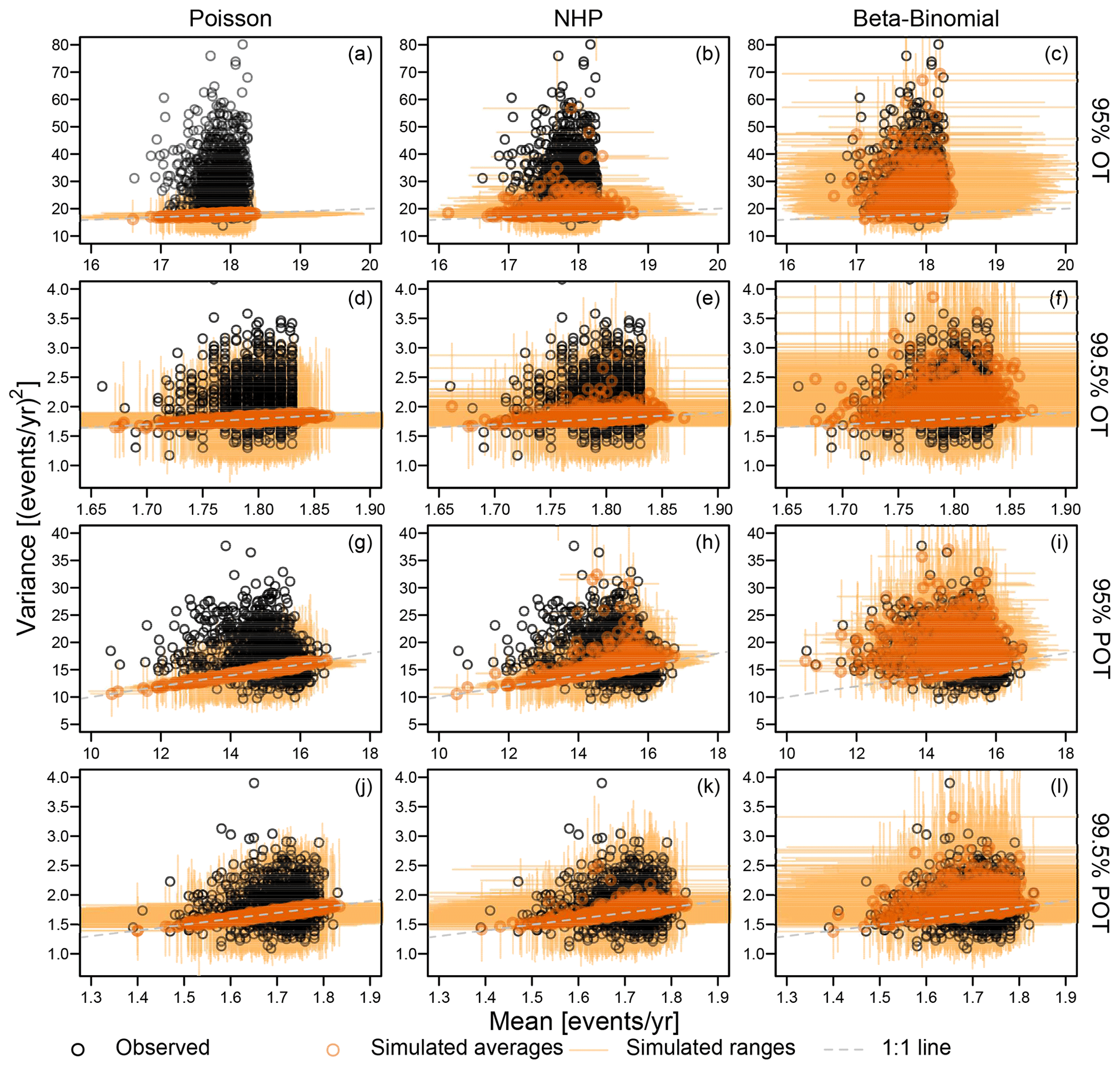
Figure 2Diagrams of sample variance versus sample mean of the annual occurrences of OT values and POT for the 95 % and 99.5 % thresholds. Observed values (in black) are compared with those corresponding to simulated samples from Poisson, NHP, and beta-binomial (βℬ) distributions (in orange). Orange circles denote ensemble averages, while horizontal and vertical segments denote the range of mean and variance values obtained over 100 simulations for each of the 1106 records. Dashed gray lines indicate the 1:1 lines representing the equality of mean and variance characteristics of Poisson distributions.
For the sake of completeness, we also considered the peaks over threshold (POT) – that is, the maximum values of independent clusters of OT values, where each cluster is considered to be a single event. Clusters are identified as sequences of positive values of daily precipitation separated by one or more dry days. Different inter-arrival times for cluster identification can be used, but this parameter is secondary in the present context.
The Poisson distribution might be a valid asymptotic model for peaks over high thresholds under suitable conditions (e.g., Davison and Smith, 1990), whereas there is no theoretical argument supporting its validity for OT data, especially if they are expected to be dependent and if the used threshold is not very high. Sample means and variances of POT show a behavior closer to Poisson and NHP models for both thresholds (Fig. 2g–l). However, Poisson and NHP models still under-represent the observed variances for the 95 % threshold, while βℬ distributions provide a faithful reproduction. According to the foregoing theoretical remarks, this is not surprising as the 95 % threshold is not high enough to identify independent events, resulting in occurrences that are still temporally dependent. As expected, the observed mean and variances of POT start to exhibit a Poissonian behavior only for the high 99.5 % threshold. In this case, both NHP and βℬ provide results close to those of the Poisson distribution as the parameters accounting for nonstationarity in NHP and autocorrelation in βℬ tend towards zero, and these models converge to the Poisson distribution, which is a special case of both.
Since Poisson and NHP provide similar results in terms of VMR for all cases, we retain the former and use probability plots (probability versus quantiles) to further check the agreement between observed data and models. We compare ECDFs Fn(z) with the CDFs F𝒫(z) and Fβℬ(z) of the Poisson and βℬ models, respectively. Probability plots are complemented with diagrams of the differences versus z. For the 95 % threshold, Fig. 3a and b show that the Poisson distribution cannot account for the observed variability in the empirical distributions, while βℬ models cover the range of variability thanks to the additional parameter summarizing the intra-block autocorrelation. This is consistent with the interpretation of over-dispersion as an effect of temporal dependence already highlighted in Fig. 2. The diagrams of δ(z) versus z in Fig. 3e and f confirm that the βℬ models are closer to the empirical distributions for a wider range of Z values compared with Poisson. For the 99.5 % threshold, we have similar results (Fig. 3c, d, g, and h), indicating that the temporal dependence of the generating processes Y still plays a role despite the apparently low correlation of Z time series.
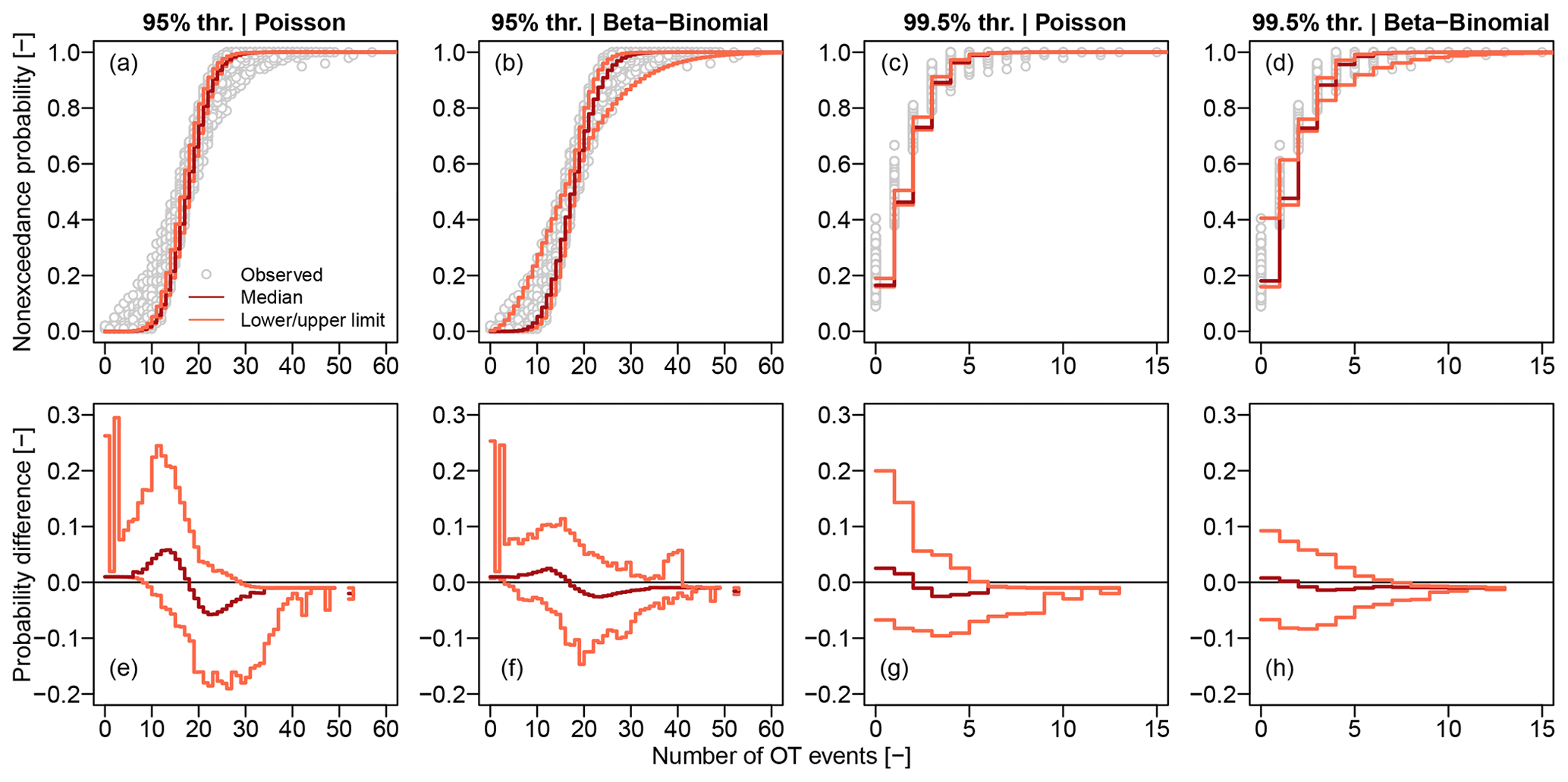
Figure 3Panels (a)–(d) show the ECDFs of Z for the 95 % and 99.5 % thresholds and for each of the 1106 rain gauges. ECDFs are complemented with the median, lower, and upper limits of the ensemble of the Poisson and beta-binomial (βℬ) models corresponding to each rain gauge. Panels (e)–(h) show the median, lower, and upper limits of the differences δ(z) between ECDFs and Poisson and βℬ distributions. Median, lower, and upper values are computed point-wise for each value z of the number of OT events Z.
The outcome of our exploratory analysis disagrees with results of goodness-of-fit tests reported by Farris et al. (2021), who concluded that the hypothesis of the Poisson distribution for Z cannot be rejected in more than 95 % of the gauges at αglobal=0.05 for all values of the percentage threshold and number of years. Therefore, we applied the three goodness-of-fit tests described in Sect. 4.1 to double-check the results of our exploratory analysis and to allow a direct comparison. Figure 4 shows the FDR diagrams reporting the sorted p values versus their ranks (Wilks, 2016, Fig. 3). The number of p values underneath the reference FDR line, which represent significant results according to the FDR control level αFDR=0.10 (Wilks, 2016), strongly depends on the specific test and threshold used. For the 95 % threshold, the FDR rejection rates are 21 %, 3 %, and 53 % for KS, PPMCC, and VMR tests, respectively. For the higher 99.5 % threshold, the number of events decreases, and OT values tend to correspond to POT. Therefore, the rejection rates decrease, becoming 1 %, 0.1 %, and 12 % for KS, PPMCC, and VMR tests, respectively. As anticipated in Sect. 4.1, these results highlight that the choice of statistical tests characterized by different powers can lead to completely different and ambiguous conclusions.
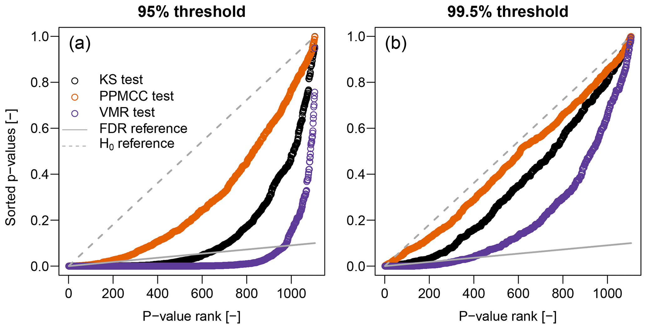
Figure 4Illustration of FDR criterion for αFDR≅0.10 (diagonal gray line) corresponding to αglobal≅0.05 (Wilks, 2016). Plotted points are the sorted p values of 1106 local tests for KS, PPMCC, and VMR tests. Points below the diagonal lines represent significant results (i.e., rejections of ℍ0) according to FDR control level.
Therefore, the theoretical arguments discussed in Sect. 4.1 and the foregoing exploratory analysis indicate that the βℬ distribution might be a good candidate distribution to describe Z, while neither Poisson nor NHP are suitable options. This calls into question the use of the Poisson-INAR(1) model as a stationary dependent reference to be used in the subsequent trend analysis. Note that the emergence of the βℬ distribution is inherently related to the assumption of serial dependence. In other words, even though we can build autocorrelated processes with whatever marginal distribution, and even though these models (e.g., Poisson-INAR(1)) can be technically correct from a mathematical standpoint, they are not necessarily consistent with the studied process. In the present case, theoretical reasoning tells us that the distribution of Z over finite-size blocks under the assumption of temporal dependence is over-dispersed and cannot be Poissonian. It follows that autocorrelated processes with Poisson marginal distributions are known in advance to be unsuitable for these OT processes; albeit, they can be mathematically correct and suitable in other circumstances.
It is also worth noting how simple diagnostic plots supported by theoretical arguments concerning the stochastic properties of the studied process provide more information than the binary output (rejection or no rejection) of whatever statistical test and also help with the identification of consistent models. On the other hand, statistical tests might be misleading. They suffer not only from several logical and technical inconsistencies but also from trivial problems related to the their choice (see discussion in Sect. 6.1). In fact, while KS, PPMCC, and VMR tests seem to be suitable choices, they have very different power for the specific problem at hand and can lead to contrasting conclusions without providing insights into the actual nature of the investigated process.
5.2 Stationary or nonstationary models?
5.2.1 Linear correlation versus linear trends: practical consequences of confusing assumptions with models
The test-based approach led Farris et al. (2021) to discard temporal dependence as a possible cause of apparent trends in Z time series based on disagreement between trend slopes estimated using observed data and Poisson-INAR(1)-simulated samples. In particular, their conclusion is based on diagrams of the lag-1 autocorrelation coefficient versus the slope of the linear trend estimated based on observed Z time series and sequences simulated by NHP and Poisson-INAR(1). Since the foregoing exploratory analysis indicated that the NHP and Poisson-INAR(1) models are not consistent with the marginal distributions of Z, we used IAAFT samples as a more realistic alternative.
Figure 5a compares the observed pairs with those resulting from the Poisson-INAR(1) models. Figure 5a is similar to Fig. 4a in Farris et al. (2021), which compares observed pairs with those corresponding to independent Poisson variables. Figure 5a confirms that the Poisson-INAR(1) models do not provide a good description of the observed behavior, as expected for models that cannot even reproduce marginal distributions. On the other hand, the pattern of the pairs estimated from IAAFT samples matches that of the observed pairs much better (Fig. 5b).
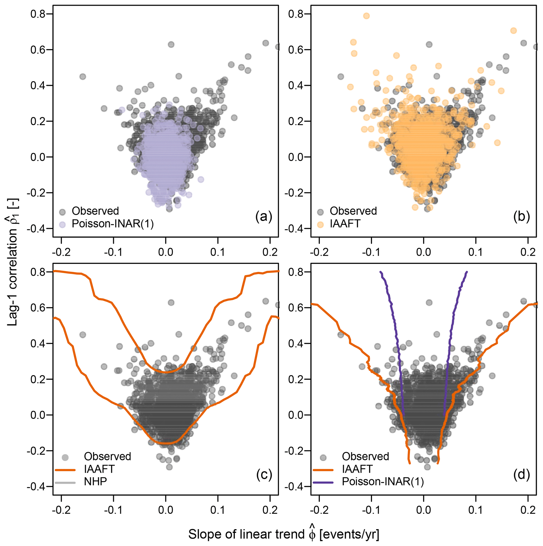
Figure 5Scatterplots of the pairs for the 1106 observed Z time series over the 95 % threshold and over 100 years (1916–2015), along with pairs corresponding to Poisson-INAR(1) samples (a), pairs corresponding to IAAFT samples (b), 95 % CIs of for IAAFT and NHP (c), and 95 % CIs of for IAAFT and Poisson-INAR(1) (d).
Following Farris et al. (2021), we also simulated 10 000 samples from (i) the NHP model for fixed values of ϕ ranging between −0.2 and 0.2, (ii) Poisson-INAR(1) for ρ1 ranging between 0 and 0.8, and (iii) IAAFT. The 10,000 samples from the three models allow the estimation of two different conditional probabilities – that is, and , respectively. Therefore, we can estimate the confidence intervals (CIs) of the conditional variables for NHP and for Poisson-INAR(1). Figure 5c and d show these point-wise CIs. Even though their comparison in unfair since they refer to different conditional distributions, Farris et al. (2021) discarded Poisson-INAR(1) as the CIs of for NHP cover the observed pairs better than the CIs of .
However, as mentioned in Sect. 4.2, if a specific model in the class of stationary models does not fit well, this does not enable us to discard the entire class. In fact, the conditional CIs of built from the IAAFT samples indicate that alternative stationary processes can yield results similar to NHP. On the other hand, IAAFT CIs of are much wider than those from Poisson-INAR(1) samples, thus confirming that such a model is clearly inappropriate to describe Z. Therefore, the class of dependent stationary models and the assumption of stationarity cannot be discarded based on the poor performance of a single misspecified stationary model that does not even reproduce the marginal distribution of the observed data.
The foregoing analysis is complemented by an additional one focusing on sub-samples. Following Farris et al. (2021), we sampled Z values recorded every 4 years, thus extracting four sub-series of size 25 and therefore removing the effect of potential autocorrelation at lags from 1 to 3 years. For each sub-sample, we estimated the linear trend slopes (with ) and plotted these against the slope estimated based on the full series.
Figure 6a and b reproduce Fig. 5 in Farris et al. (2021). Figure 6a shows the scatterplot of the pairs of the observed Z, while Fig. 6b displays the pairs for synthetic series from the NHP model. The similarity of the patterns led Farris et al. (2021) to conclude that the serial dependence does not play any significant role, and observed trends are consistent with NHP behavior. However, the additional Fig. 6c shows that the pairs from stationary and temporally correlated IAAFT samples also exhibit behavior similar to that of the observed Z, thus contradicting the foregoing conclusion.
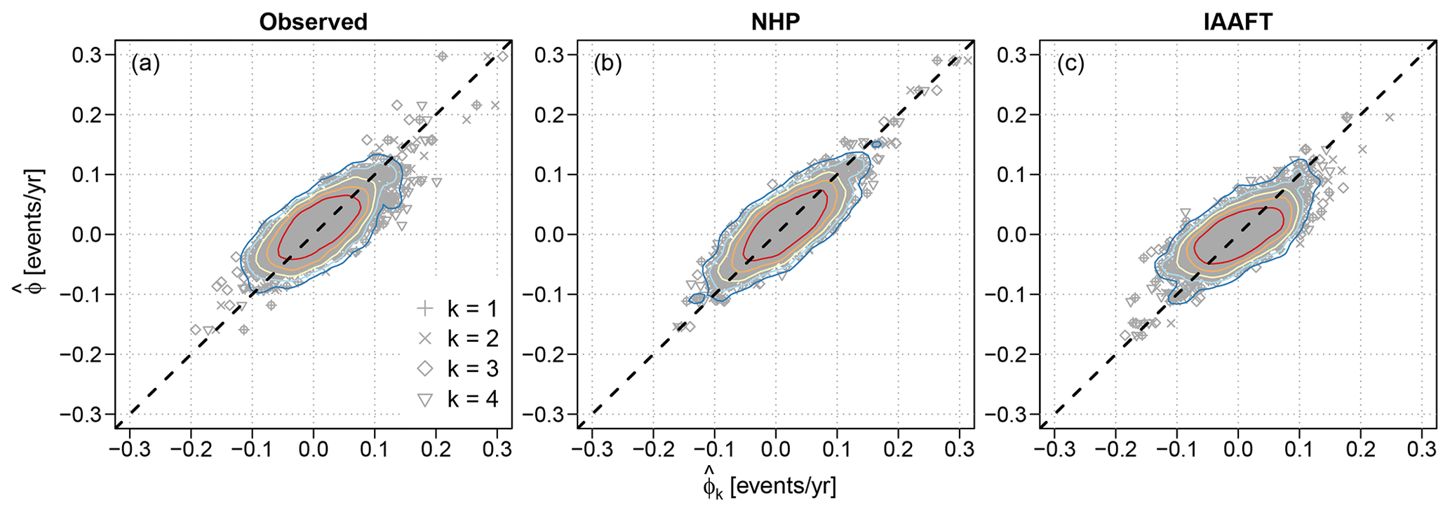
Figure 6(a) Scatterplot of the pairs , where is the slope of the linear trend estimated based on the observed Z time series for the 95 % threshold and 100 years, while (with ) is the slope estimated based on four sub-samples of lengths equal to 25 years. (b, c) Similar to (a) but for time series simulated from NHP and IAAFT, respectively.
Analogously to the analysis of pairs , the analysis of the pairs seems to be reasonable at first glance. However, it suffers from similar inconsistencies:
-
The 4-year-lagged sub-samples are supposed to be approximately independent based on the belief that the correlation is weak and that the value of ACF terms is generally low. However, this assumption misses the fact that, under dependence, the ACF estimates based on finite samples are negatively biased and need to be adjusted according to a parametric model of choice. In this respect, Fig. 5 and the corresponding Fig. 4 in Farris et al. (2021) are not even consistent because all panels show the ρ1 values obtained by standard estimators that are only valid under independence, whereas the panels referring to Poisson-INAR(1) and IAAFT should show ρ1 values adjusted for estimation bias. This further confirms that assumptions like (in)dependence and (non)stationarity influence not only the model parameterization (e.g., Poisson with or without linear trend) but also the entire inference procedure, including diagnostic plots and their interpretation.
-
The performance of a specific independent nonstationary model (NHP) is incorrectly considered to be informative about the performance of an entire alternative class of dependent stationary models, while NHP is not even defined under those alternative assumptions. The ability of NHP to reproduce the patterns of cannot exclude the existence of equally good or better models based on different assumptions. The only way to understand if a class of models (and the underlying assumptions) is suitable for a given data set is to use credible members of such a class. This conceptual mistake is the same one affecting statistical tests, where the rejection of ℍ0 is often misinterpreted and leads us to uncritically embrace the alternative hypothesis ℍ1, while rejection can be due to unknown factors that are not included in either ℍ0 or ℍ1 (see discussion in Sect. 6.1).
To summarize, our analysis shows that neither NHP nor Poisson-INAR(1) are suitable models for Z in the considered range of thresholds. On the other hand, for POT and high thresholds, we recover the theoretically expected Poissonian behavior, and NHP and Poisson-INAR(1) models tend to converge to the Poisson model, thus becoming almost indistinguishable.
5.3 Trend analysis of observed extreme-P occurrences: the actual role of spatio-temporal dependence
After analyzing marginal distributions and temporal dependence, we study spatio-temporal fluctuations of Z, comparing model-based and test-based methods. We expand the analysis of Z (number of annual OT values at each gauging location) considering the number of daily and annual OT events aggregated over the five regions described in Sect. 2 and shown Fig. 1. This allows us to check if the assumption of dependence and the corresponding models provide a reasonable description of OT frequency over a range of spatio-temporal scales.
5.3.1 Trend analysis under temporal dependence
We analyze the presence of trends in Z time series recorded at the 1106 stations selected from the GHCN gauge network. For the sake of comparison with test-based results, trends are investigated by applying the same MK and PR tests. However, the distributions of test statistics (and therefore of critical values) are estimated from 10 000 IAAFT samples to properly account for the over-dispersion of the marginal distributions and the temporal correlation. Moreover, tests are firstly performed at the local 5 % significance level without applying FDR to check if the empirical rejection rate is close to the nominal one, as expected under correct model specification.
Figures 7 and 8 show the maps of trend test results for the 95 % threshold; the 100-year sample size; and the three regions of North America, Eurasia, and Australia, with and without FDR, respectively (results for the other combinations of thresholds and sample sizes with and without FDR are reported in Figs. S2–S7 in the Supplement). Results in Figs. 7 and 8 are different from those reported by Farris et al. (2021) in their analogous Fig. 9. To better understand such differences, we examine the rejection rates of both MK and PR tests for the four combinations of two thresholds (95 % and 99.5 %) and two sample sizes (50 and 100 years) and four different cases: (𝒜) critical values of test statistics obtained by IAAFT without bias correction of the autocorrelation and without FDR, (ℬ) critical values obtained by IAAFT with bias correction and without FDR, (𝒜FDR) critical values obtained by IAAFT without bias correction and with FDR, and (ℬFDR) critical values obtained by IAAFT with bias correction and FDR (Table 1). Case ℬ highlights the effect of adjusting for the bias of classical ACF estimators under the assumption of temporal dependence, while cases 𝒜FDR and ℬFDR show the effects of spatial correlation (albeit indirectly via FDR).
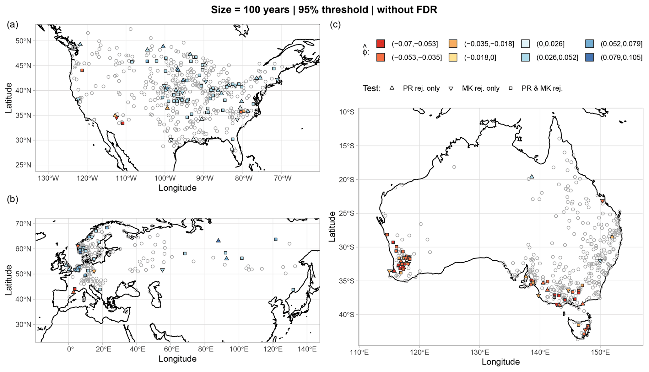
Figure 7Maps of statistically significant trends at the GHCN gauges of the three regions of North America (a), Eurasia (b), and Australia (c). Results refer to MK and PR tests applied to Z time series for the 100-year sample size and the 95 % threshold without FDR. Statistical tests are performed at the local 5 % significance level without applying FDR. The distributions of test statistics (and therefore critical values) are estimated from 10 000 IAAFT samples. Gray circles denote lack of rejection by both tests. Results for the other combinations of thresholds and sample sizes are reported in Figs. S2–S4 in the Supplement.
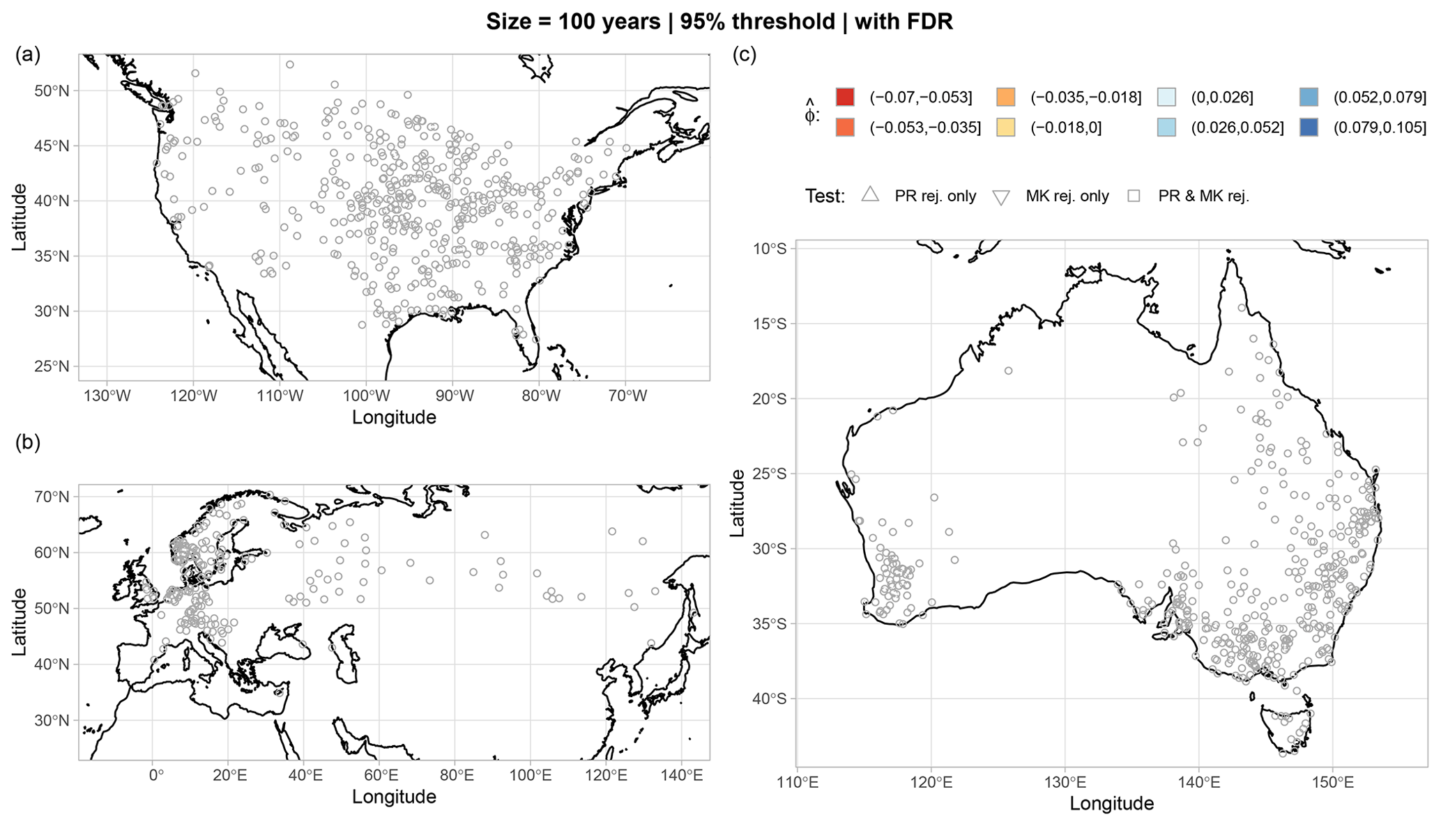
Figure 8Similar to Fig. 7 but with FDR. Results for the other combinations of thresholds and sample sizes are reported in Figs. S5–S7 in the Supplement.
Table 1Rejection rates of PR and MK tests for the four combinations of two thresholds (95 % and 99.5 %) and two sample sizes (50 and 100 years) and different treatments of spatio-temporal dependence (cases 𝒜={Biased ACF | w/o FDR}, ℬ={Bias adjusted ACF | w/o FDR}, 𝒜FDR={Biased ACF | w/ FDR}, and ℬFDR={Bias adjusted ACF | w/ FDR}).
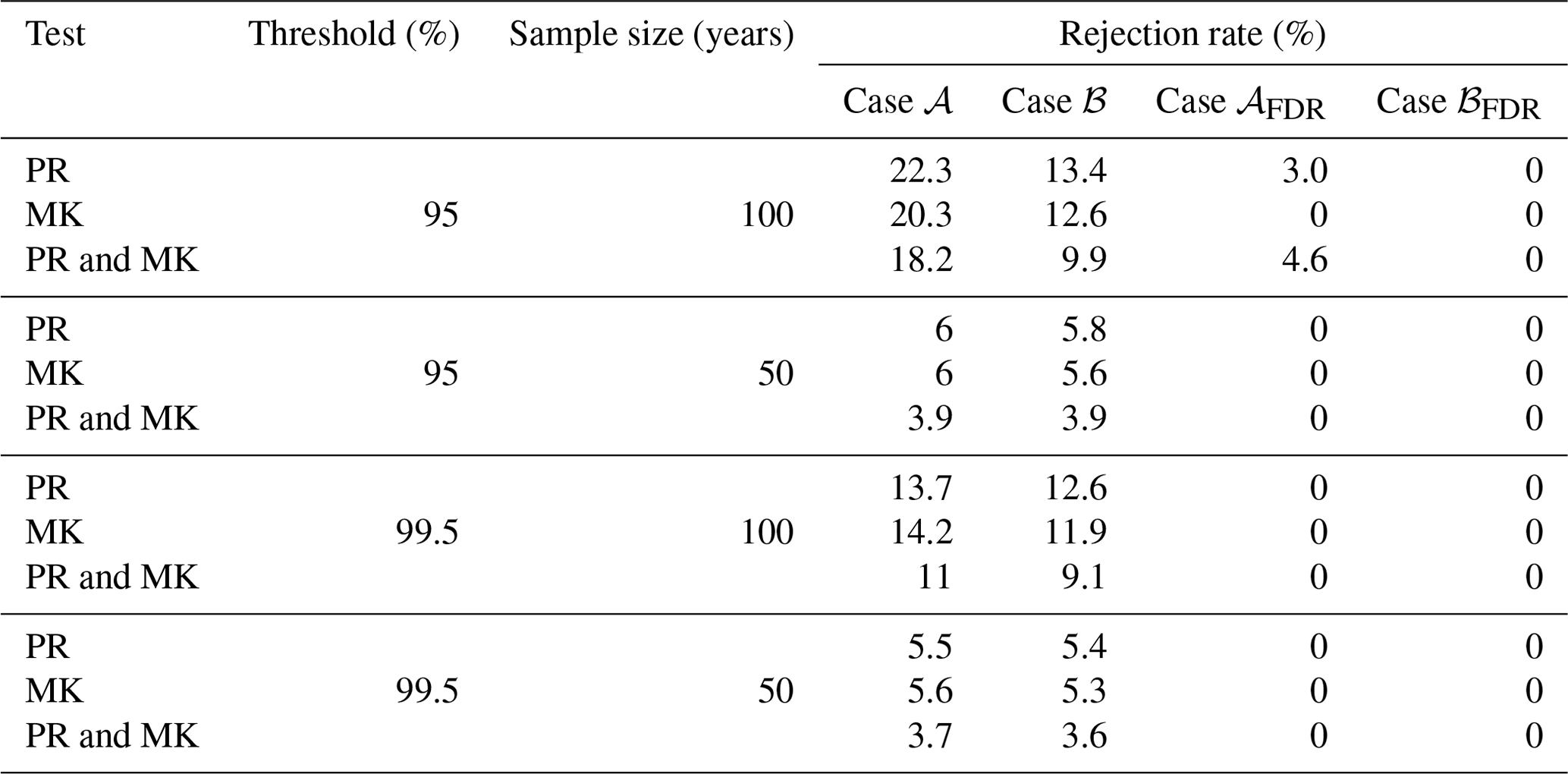
Focusing on case 𝒜, for 50-year time series, local rejection rates are always close to the nominal 5 %, as expected. For 100-year time series, local rejection rates corresponding to the 95 % and 99.5 % thresholds reach a maximum of 22 % and 14 %, respectively. These values seems to be higher than expected. However, after correcting ACF bias (case ℬ), the maximum rejection rate for the 95 % threshold drops to 13 %, whereas the rejection rates for the 99.5 % threshold stay almost unchanged. This is due to the higher (lower) autocorrelation of OT values corresponding to lower (higher) thresholds and, therefore, stronger (weaker) bias correction. Overall, accounting for ACF bias results in rejection rates ranging between 9 % and 13 %. After considering (indirectly) the effects of spatial correlation via FDR (cases 𝒜FDR and ℬFDR), the rejection rate drops to zero in all cases if we correct ACF bias (case ℬFDR), meaning that all tests are globally not significant at αFDR≅0.10. If we do not adjust ACF bias (case 𝒜FDR), a small percentage of tests indicate global significance at αFDR≅0.10 for a sample size of 100 and a threshold equal to 95 %. This is expected as the correction of ACF bias is more effective for larger sample sizes and lower thresholds. In fact, decreasing thresholds generally correspond to an increasing temporal correlation of Z samples, and larger samples allow a better quantification of the properties of a correlated process.
Some simple diagnostic plots can provide a clearer picture. Figure 9 shows the scatterplots of the pairs , with the rejections highlighted by different markers. Figure 9 is analogous to Fig. 10 in Farris et al. (2021) but using IAAFT samples and considering the cases 𝒜, ℬ, 𝒜FDR, and ℬFDR. It shows how the number of rejections decreases as the effects of temporal and spatial correlation are progressively compounded. Focusing on case ℬ, rejections tend to occur for higher values of conditioned to the value of , but there is no systematic rejection for all exceeding a specified value, as for the case 𝒜. On the contrary, the pairs marked as rejections overlap with the pairs marked as no rejection, indicating that we can have both rejections and no rejections for time series with similar values of and .
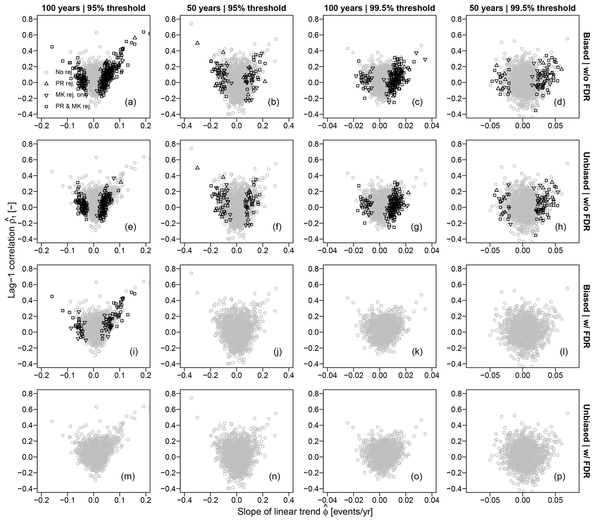
Figure 9Scatterplots of the pairs , with the rejections highlighted by different markers. Markers refer to rejections of the MK test, PR test, or both for Z time series corresponding to the four combinations of two thresholds (95 % and 99.5 %) and two sample sizes (50 and 100 years) and the three cases 𝒜={Biased ACF | w/o FDR}, ℬ={Bias adjusted ACF | w/o FDR}, 𝒜FDR={Biased ACF | w/ FDR}, and ℬFDR={Bias adjusted ACF | w/ FDR}. Gray circles denote lack of rejection by both tests.
These results disagree with those reported by Farris et al. (2021), who found that the hypothesis of a significant trend is always rejected for events per year and concluded that “the occurrence of the different cases is controlled by , while is not influential, thus providing additional evidence on the limited effect of autocorrelation on trend detection”. However, those rejections result from MK and PR tests performed under the assumption of temporal independence (case ρ=0; φ=0 in Farris et al., 2021). In this case, rejections are necessarily independent of due to the implicit model under which the tests are performed. As recalled in Sect. 1, results should be interpreted in light of the underlying statistical model and not vice versa.
As mentioned throughout this study, a suitable diagnostic plot might be more informative than just reporting the number and/or rate of rejections. Figure 10 displays the FDR diagrams of the sorted p values versus their ranks for MK and PR tests. All p values are above the FDR reference line. Independently of the geographic region one focuses on, all tests are not significant at αFDR≅0.10, and ℍ0 cannot be rejected at the global level. Moreover, FDR diagrams provide additional information. In fact, when ℍ0 is consistent with the underlying (implicit or explicit) model and corresponding assumptions, p values are expected to be uniformly distributed – that is, aligned along a straight line connecting the origin (0,0) and the point with abscissa equal to the maximum rank and ordinate equal to the maximum p value, where the latter is equal to 1 (0.5) for one-sided (two-sided) tests (e.g., Falk and Michel, 2006; Serinaldi et al., 2015). Figure 10 shows that the estimated p values are reasonably aligned along such a line, thus confirming the overall (global) consistency of ℍ0 with a temporally correlated and over-dispersed process for Z.
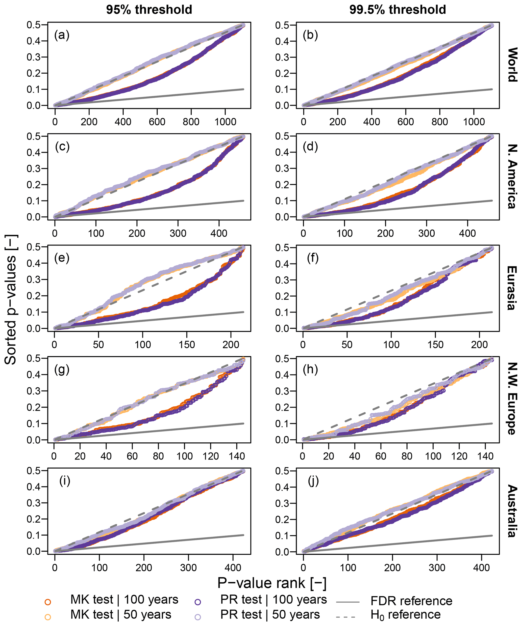
Figure 10Illustration of FDR criterion with αFDR≅0.10 (diagonal gray line). Plotted points are the sorted p values resulting from the application of MK and PR tests to data recorded at each location. Results are reported for the five regions described in Sect. 2. The distributions of test statistics (and therefore critical values) are estimated from 10 000 IAAFT samples. Points below the diagonal lines represent significant results (i.e., rejections of ℍ0) according to FDR control levels.
5.3.2 Space beyond time: the non-negligible effects of spatial dependence
Figure 7 (and Figs. S2–S4 in the Supplement) shows that the locally significant trends tend to cluster in geographic areas where such trends exhibit the same sign (e.g., southwestern Australia, North America, and European coastal areas around the North Sea). Often, this behavior is interpreted as further evidence of trend existence. However, this interpretation neglects the fact that the spatial clustering is also an inherent expression of spatial dependence in the same way temporal clustering is the natural expression of temporal dependence (see, e.g., Serinaldi and Kilsby, 2016b, 2018; Serinaldi and Lombardo, 2017a, b, 2020, for examples of spatio-temporal clustering).
For example, Farris et al. (2021) state that the detection of significant trends with similar signs or magnitudes over spatially coherent areas “is also supported by the physical argument that extreme P is often controlled by synoptic processes (Barlow et al., 2019), and that their occurrence is changing in time (Zhang & Villarini, 2019)”. However, while a similar evolution of the occurrence of extreme P and synoptic systems is due to their physical relationships, statistical tests for trends cannot provide information about the nature of the temporal evolution of such processes. Indeed, as shown in Sect. 5.3.1, the outcome of statistical tests depends on the underlying assumptions. Therefore, the jointly evolving fluctuations of both processes (extreme P and synoptic systems) can be identified as not significant or significant based on the assumptions used to perform the statistical tests. Loosely speaking, if we observe an increasing trend in the occurrence of synoptic systems, a similar behavior is likely to emerge in local P records observed over the area where the synoptic processes occur as the latter causes the former. Therefore, what we actually need is to identify the physical mechanism causing trends in the synoptic systems as trends in extreme P are just a consequence. In this respect, performing massive statistical testing is rather uninformative as it does not matter whether the observed fluctuations are statistically significant or not. Detecting trends in multiple local processes that are known to react to fluctuations in synoptic generating processes does not add evidence and just reflects information redundancy due to their common causing factor.
To support the foregoing statements with quantitative analysis, we checked the consistency of the spatio-temporal behavior of observed OT occurrences with the assumption of spatio-temporal dependence. Following the model-based approach, we avoid statistical tests for trend detection and rely on theoretical reasoning to formulate a coherent model, thus checking the agreement with observations by means of simple but effective diagnostic plots.
We firstly check the role of the possible spatial dependence of OT occurrences, focusing on the distribution of the number ZS of daily OT occurrences over the five regions introduced in Sect. 2 (i.e., the world, North America, Eurasia, northwestern Europe, and Australia). A daily timescale is selected to isolate the effect of spatial dependence from that of temporal dependence as it is the finest timescale, and the counting procedure does not involve any aggregation over time. The occurrence of OT events over m locations can be seen as the outcome of m Bernoulli trials. Under dependence, the distribution of ZS can be described by a βℬ distribution, where the parameter ρβℬ controlling over-dispersion can be expressed as the average of the off-diagonal terms of the lag-0 correlation matrix of the process Y describing the daily occurrence or non-occurrence of OT events at each spatial location (see Sect. S4 in the Supplement). In other words, if the spatial correlation is sufficient to describe the spatial clustering, we expect that the βℬ distribution with ρβℬ estimated as the average cross-correlation between binary time series of daily OT occurrences faithfully matches the empirical distribution of ZS over any region.
Figure 11 shows that the βℬ distribution reproduces accurately the above-mentioned empirical distributions for any threshold and region. Note that North America, Eurasia, Australia, and northwestern Europe are nested regions of the world, and northwestern Europe is also a nested region of Eurasia. Therefore, the remarkable fit of βℬ indicates that the spatial correlation is sufficient to describe the spatial clustering both globally and locally. In other words, the simultaneous occurrence of daily OT events in North America or northwestern Europe, for instance, is consistent with a stationary spatially correlated process. Figure 11 also reports the binomial distribution that would be valid under independence, thus highlighting the huge (but too often neglected) impact of spatial dependence on the distribution of ZS (see also Douglas et al., 2000; Serinaldi and Kilsby, 2018; Serinaldi et al., 2018, for additional examples).
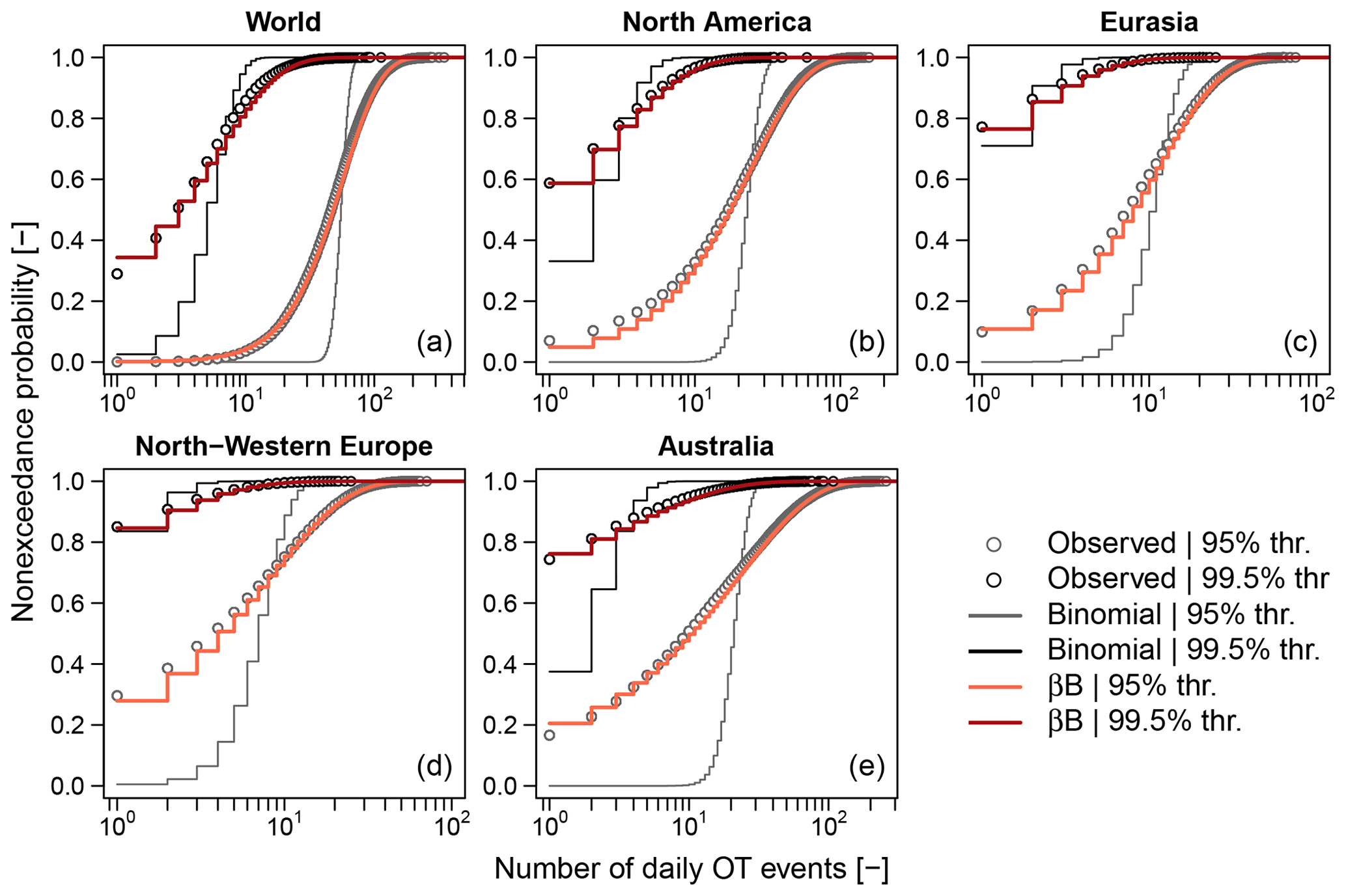
Figure 11ECDFs of number of OT events (for the 95 % and 99.5 % thresholds) occurring at a daily timescale over different regions, along with binomial and βℬ CDFs.
Since the aim of tests for trends should be the detection of “deterministic” temporal patterns, we checked the possible temporal evolution of the distribution of ZS over the five regions. This information is summarized in Fig. 12 in terms of boxplots of ZS aggregated at a decadal scale to better visualize temporal patterns along the century. Figure 12 also shows the 95 % prediction intervals from binomial and βℬ distributions reported in Fig. 11. Of course, these prediction intervals are constant as the binomial and βℬ distributions are unique under the assumption of stationarity. The empirical distributions of ZS do not show any evident temporal evolution throughout the 10 decades, and more importantly, any possible fluctuation is well within the range of values allowed by the βℬ distribution. The comparison of the 95 % prediction intervals from binomial and βℬ models further highlights the huge effect of spatial dependence, which can yield prediction intervals from ≅2 up to ≅6 times wider than those corresponding to spatial independence.
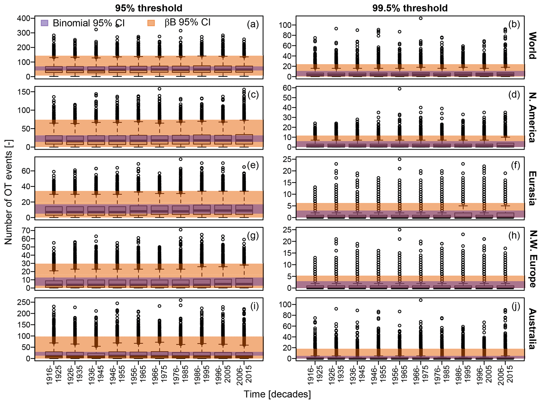
Figure 12Boxplots summarizing the decadal distributions of the number of OT events (for the 95 % and 99.5 % thresholds) occurring at a daily timescale over different regions, along with the 95 % prediction intervals corresponding to binomial and βℬ distributions.
5.3.3 Space and time: the non-negligible effects of spatio-temporal dependence
While the analysis at a daily scale allowed us to focus on spatial dependence, here we focus on the annual number ZST of OT events over multiple locations. Studying the spatial clustering of such data implies aggregation in space and time. In other words, the occurrence of OT events can be thought of as a set of Bernoulli trials over m locations (i.e., the number of stations in each geographic region) and n time steps (i.e., the 365 d in a 1-year time interval), and we are interested in the distribution of ZST resulting from m⋅n Bernoulli trials. This case is analogous to that concerning daily OT occurrences. The βℬ distribution is still a theoretically consistent model for ZST, and its over-dispersion parameter ρβℬ can be expressed as the average of all lagged auto- and cross-correlation values of the generating binary process Y up to time lag n=365 (see Sect. S4 in the Supplement). As with the case of spatial dependence, we use probability plots and boxplots to assess the validity of the βℬ distribution and, therefore, its underlying assumption of spatio-temporal dependence.
Figure 13 shows that the βℬ model faithfully describes the ECDFs of ZST for any threshold and region. This means that the local spatio-temporal correlation is sufficient to describe the differences in all regions and sub-regions without introducing any ad hoc local models involving, for instance, physically unjustified linear trends or generic links with local exogenous factors. We stress again that the parameter ρβℬ is not estimated based on the 100 values of ZST in each region; instead, it comes from the spatio-temporal correlation values of the generating binary process Y. Therefore, the goodness of fit of the βℬ distribution is not related to the minimization of some distance metric for 100-size samples but depends on the agreement of the observed binary time series with the hypothesized stationary spatio-temporal stochastic process Y.
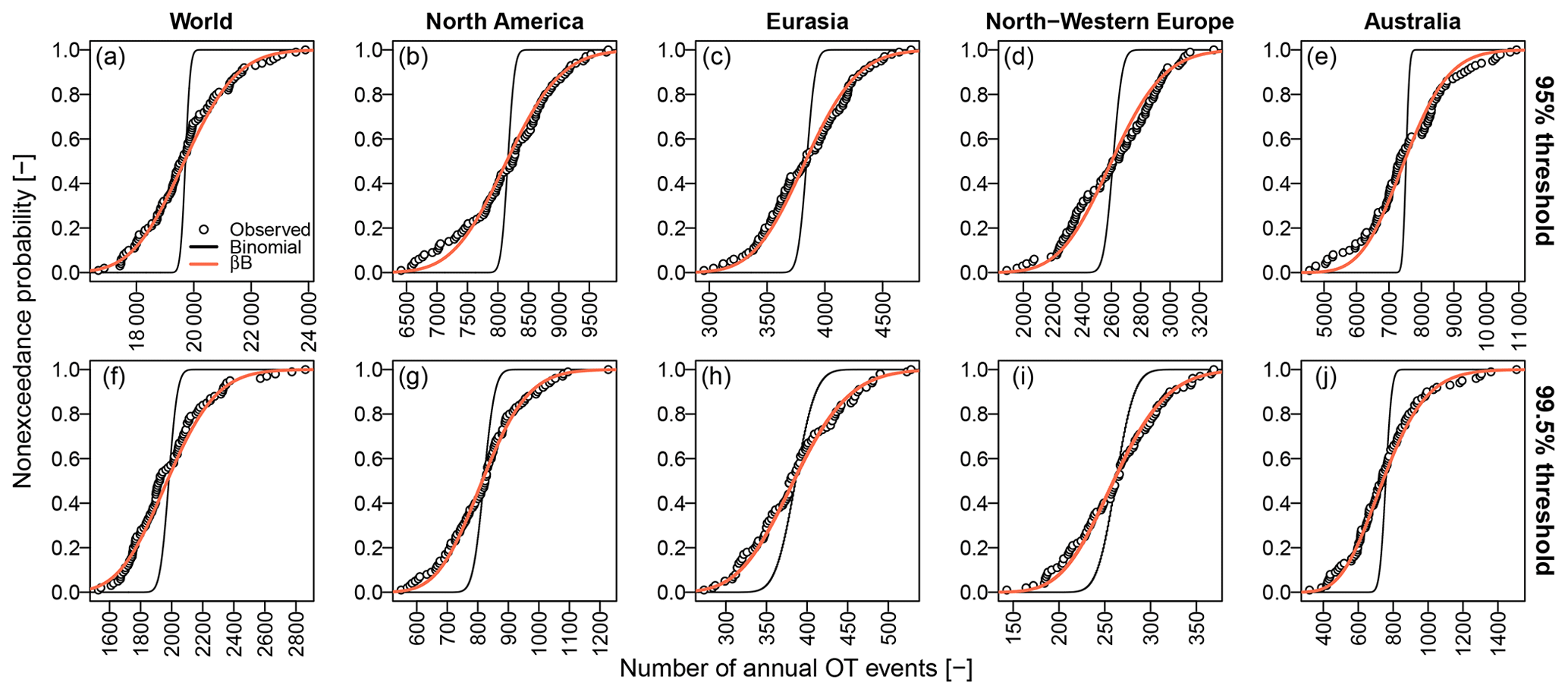
Figure 13ECDFs of number of OT events (for the 95 % and 99.5 % thresholds) occurring at an annual timescale over different regions, along with binomial and βℬ distributions.
For any threshold and region, Fig. 14 confirms that the temporal fluctuations of the distribution of ZST are well within the range of values expected from a stationary stochastic process characterized by the observed spatio-temporal correlation structure. In this case, the 95 % prediction intervals from βℬ models under spatio-temporal dependence are from ≅3 up to ≅13 times wider than those yielded by binomial distribution under spatio-temporal independence. Of course, an increasing pattern along the decades is evident in the regions of the Northern Hemisphere. However, accounting for spatio-temporal correlation dramatically changes their interpretation. Such fluctuations are obviously inconsistent with the assumption of independence and, therefore, the binomial model. This explains the high rejection rate of the trend tests performed under independence. On the other hand, low-frequency fluctuations evolving over wide spatial scales and timescales comparable to or longer than the observation period are the expected behavior of spatio-temporally dependent processes. Therefore, we should ask ourselves whether such fluctuations can look unexpected or surprising because they are actually unusual or just because humans tend to systematically underestimate the actual uncertainty characterizing the surrounding environments, thus looking at hydro-climatic processes with a too-anthropocentric point of view, which is inherently uncertainty-averse or behaviorally biased towards known outcomes.
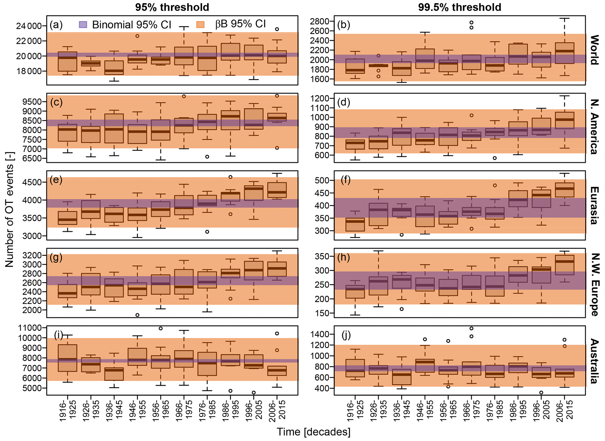
Figure 14Boxplots summarizing the decadal distributions of the number of OT events (for the 95 % and 99.5 % thresholds) occurring at an annual timescale over different regions, along with the 95 % prediction intervals corresponding to binomial and βℬ distributions.
6.1 Statistical tests for trend detection: unfit for purpose!
Disagreements between model-based and test-based methods are mainly related to the inherent problems affecting statistical hypothesis tests. These are statistical methods developed for the evaluation of differences in repeatable experiments that “have been misused to create an illusion of a scientific analysis of unrepeatable hydrologic events” (Klemeš, 1986). Logical, conceptual, and practical inconsistencies in statistical tests have been widely discussed in both theoretical and applied literature (Pollard and Richardson, 1987; Gigerenzer et al., 1989; Flueck and Brown, 1993; McBride et al., 1993; Meehl, 1997; Gill, 1999; Johnson, 1999; Nicholls, 2001; Krämer and Gigerenzer, 2005; Levine et al., 2008; Ambaum, 2010; Clarke, 2010; Beninger et al., 2012; Ellison et al., 2014; Nuzzo, 2014; Briggs, 2016; Greenland et al., 2016; Wasserstein and Lazar, 2016; Serinaldi et al., 2018, 2020a; Wasserstein et al., 2019, and references therein).
One of the key drawbacks of statistical tests is the error of the “transposed conditional” (also known as the “converse inequality argument” or “inverse-probability problem” (Pollard and Richardson, 1987; Gill, 1999; Krämer and Gigerenzer, 2005; Ambaum, 2010; Beninger et al., 2012; Serinaldi et al., 2018, 2022)). This consists of confusing conditional and conditioning events so that we are interested in the probability of the null hypothesis ℍ0 given the observational evidence (data); hence, we end up calculating the probability observational data when ℍ0 is assumed to be true. This is like confusing the probability ℙ [a man is a UK citizen | a man is the King of the UK] ≅1 with the probability ℙ [a man is the King of the UK | a man is a UK citizen] .
In the context of statistical tests for trend detection applied to hydro-climatic data, the rejection of ℍ0 (e.g., no trend) does not provide information about the likelihood of ℍ0 given the observations. Rejection does not allow any statement about possible deterministic trends because deterministic trends are not a property of the model ℍ0 assumed to perform the test. In other words, rejection can be due to something that is unknown and different from deterministic trends. Similarly, no rejection might be related to the violation of implicit assumptions of the model ℍ0, thus introducing spurious effects due to exogenous factors (Serinaldi et al., 2022). One of these factors is the spatio-temporal dependence. Its effects on statistical inference have been widely studied in the literature (Jones, 1975; Katz, 1988a, b; Katz and Brown, 1991; Kulkarni and von Storch, 1995; Hamed and Rao, 1998; Douglas et al., 2000; Yue and Wang, 2002; Koutsoyiannis, 2003; Yue and Wang, 2004; Hamed, 2008, 2009a, b, 2011; Bayazit and Önöz, 2007; Serinaldi and Kilsby, 2016a, 2018; Serinaldi et al., 2018, 2020a). In particular, von Storch and Zwiers (2003, p. 97) recalled that “the use of statistical tests in a cookbook manner is particularly dangerous. Tests can become very unreliable when the statistical model implicit in the test procedure does not properly account for properties such as spatial or temporal correlation”. Nonetheless, the foregoing iterated warnings and recommendations are systematically ignored.
6.2 Models, tests, and their interpretation
The aim of most of the literature applying statistical tests for trend detection in hydro-climatic processes is to find the answer to a question that can generally be summarized as “are these processes stationary or nonstationary?”. However, such a question is scientifically ill-posed as natural processes cannot be either stationary or nonstationary. Only mathematical models used to describe physical processes can be one or the other.
It can be argued that “statistical trend testing attempts to assess whether the natural process has manifested in a stationary or nonstationary fashion during the period of observation to ultimately support decision-making in the future”. However, this type of statement confuses sampling fluctuations, which can look monotonic or not, with a population property such as stationarity. Statistical trend tests attempt to infer the latter as theoretical properties or assumptions are the only one behind any statistical method. As with every statistical method, statistical tests for trend detection make inferences about “population stationarity” (Khintchine, 1934; Kolmogorov, 1938) and not about sampling fluctuations, which can result from a variety of stationary and nonstationary processes. These tests attempt to establish what kind of population behavior is compatible with observed sampling fluctuations. Otherwise, we would not need any test to state that an observed sample shows a given (monotonic or non-monotonic) temporal pattern as we would just need to look at the diagrams of time series. We infer the population properties because these allow us to assume a model and to make out-of-sample predictions. We argue that the vague use of the term “stationarity”, overlooking a formal definition and its consequences, is one the main reasons for the widespread misuse and misinterpretation of the output of statistical tests (see Koutsoyiannis and Montanari, 2015; Serinaldi et al., 2018, and Sect. S3 in the Supplement for further discussion).
The comparison of test-based and model-based approaches discussed in this study attempts to clarify the foregoing concepts. For the same physical process (i.e., the OT occurrences of P), we showed two options. On the one side, we can choose to model the number Z of OT occurrences by nonstationary Poisson distributions (NHP). In this way, (i) we neglect the fact that the Poisson distributions are theoretically unsuitable to describe Z and, therefore, do not reproduce the observed marginal distribution of the Z process, and (ii) we assume that the rate of occurrence in NHP models changes in time according to linear (or nonlinear) laws that have no physical justification. The aim of these types of regression models is exactly to follow sampling fluctuations, and they hardly ever provide information about the underlying population properties. This also explains why extrapolation for these types of models is always deprecated in textbooks and introductory courses in statistics, and why, when it is done, it might yield paradoxical results (Serinaldi and Kilsby, 2015; Luke et al., 2017; Iliopoulou and Koutsoyiannis, 2020; Anzolin et al., 2024). On the other side, we can attempt to preliminarily understand the general theoretical properties of spatio-temporal OT processes, look for appropriate models reproducing such expected population properties, and check if these models are general enough to reproduce the observations at various spatio-temporal scales. Using this approach, we ended up with the conclusion that the spatio-temporal correlation structure of a stationary stochastic process provides a good description of the behavior of the observed OT frequencies at various spatio-temporal scales. Thus, the actual question is not about the (non)stationarity of natural processes or “(non)stationary behavior of observed samples” but rather which kind of model we deem to be more suitable in terms of generality, reliability, and parsimony.
Conversely to what is often iterated in the literature, accurate statistical trend analyses of observed and modeled P time series are not key to validate hypotheses regarding the underlying physical mechanisms and do not improve our ability to predict the magnitude of these changes. On the contrary, the foregoing discussion shows that the statistical tests for trend detection might generate confusion, potentially concealing model misspecification (see also Serinaldi and Kilsby, 2016a; Serinaldi et al., 2018, 2020a, 2022, for further examples). Statistical tests can just reflect the properties of the underlying models at most, while well-devised models do not need any statistical test to be validated. In fact, we did not use any statistical test to show the validity of the model-based approach. We only needed to visually compare observed properties with those expected from the theory for a range of spatio-temporal scales. When we applied statistical tests for the sake of comparison with the existing literature, the tests' outcomes just reflected what was already known and expected from a theoretical point of view.
6.3 Confirmatory versus disconfirmatory empiricism
Why do our results contrast with those reported in most of the existing literature on trend detection? The reason is that most of this literature resorts to methods based on the same unrealistic assumption of independence and corresponding trivial models such as those discussed in this study. On the other hand, when dependence is accounted for, its true consequences for the entire inference procedure are commonly underestimated, partially missed, or neglected (e.g., Lombardo et al., 2014; Koutsoyiannis, 2020; Dimitriadis et al., 2021, and references therein). Therefore, the resulting (expected) high rejection rates are incorrectly interpreted as evidence of a specific alternative, whereas rejection can be due to a variety of causes that are not considered in the analysis. The missing key point is that the results of statistical analysis and their interpretation depend on the underlying assumptions and models according to the rationale of statistical inference (Aitken, 1947; Cramér, 1946; Papoulis, 1991; von Storch and Zwiers, 2003). Conversely to what is too often incorrectly stated in the literature, even the simplest diagnostic diagram relies on an underlying model.
Why does most of the literature on trend detection rely on the same methods? There are several reasons. We argue that the main one is a too-superficial approach to probability and statistics, along with insufficient exposure to the epistemological principles of science. Using similar methods based on the same assumptions always gives similar results. However, “a million observations of white swans do not confirm the non-existence of black swans”, and “a million confirmatory observations count less than a single disconfirmatory one… What is called `evidence based' science, unless rigorously disconfirmatory, is usually interpolative, evidence-free, and unscientific” (Taleb, 2020). Since most of the literature on trend detection is just an iterative application of test-based approaches and, eventually, statistical tests under the assumption of independence or ill-defined dependence, one should wonder whether the general agreement is related to the common misinterpretation of the output of the same inappropriate methodologies rather than to physical properties. In this study, we offered an alternative point view, which is nothing but the specialization for data analysis of the scientific method used for centuries and seemingly forgotten in recent decades in some research areas. Obviously, according to the scientific method, the content of this study should also be taken critically, and interested readers should independently assess which approach (test-based, model-based, or something else) looks more general; reliable; parsimonious; and, eventually, consistent with the epistemological principles of scientific inquiry.
Data are freely available from the Global Historical Climatology Network repository (Menne et al., 2012a, https://doi.org/10.7289/V5D21VHZ).
The supplement related to this article is available online at: https://doi.org/10.5194/hess-28-3191-2024-supplement.
The author has declared that there are no competing interests.
Publisher's note: Copernicus Publications remains neutral with regard to jurisdictional claims made in the text, published maps, institutional affiliations, or any other geographical representation in this paper. While Copernicus Publications makes every effort to include appropriate place names, the final responsibility lies with the authors.
The author acknowledges the support from the Willis Research Network. The author thanks the handling editor, Nadav Peleg (University of Lausanne), and the eponymous reviewers, Panayiotis Dimitriadis (National Technical University of Athens), Demetris Koutsoyiannis (National Technical University of Athens), and Giuseppe Mascaro (Arizona State University), for their critical remarks that helped substantially to improve the content and presentation of the original draft of the paper. The author also thanks Hans von Storch for his feedback on a previous version of this paper. The analyses were performed in R (R Development Core Team, 2023).
This paper was edited by Nadav Peleg and reviewed by Giuseppe Mascaro, Demetris Koutsoyiannis, and Panayiotis Dimitriadis.
Aitken, A. C.: Statistical mathematics, Oliver and Boyd Interscience Publishers, New York, USA, 5th edn., 1947. a, b, c
Ambaum, M. H. P.: Significance tests in climate science, J. Climate, 23, 5927–5932, 2010. a, b
Anzolin, G., de Oliveira, D. Y., Vrugt, J. A., AghaKouchak, A., and Chaffe, P. L.: Nonstationary frequency analysis of extreme precipitation: Embracing trends in observations, J. Hydrol., 637, 131300, https://doi.org/10.1016/j.jhydrol.2024.131300, 2024. a
Barunik, J. and Kristoufek, L.: On Hurst exponent estimation under heavy-tailed distributions, Physica A, 389, 3844–3855, 2010. a
Bayazit, M. and Önöz, B.: To prewhiten or not to prewhiten in trend analysis?, Hydrol. Sci. J., 52, 611–624, 2007. a
Beninger, P. G., Boldina, I., and Katsanevakis, S.: Strengthening statistical usage in marine ecology, J. Exp. Marine Biol. Ecol., 426–427, 97–108, 2012. a, b
Benjamini, Y. and Hochberg, Y.: Controlling the false discovery rate: A practical and powerful approach to multiple testing, J. Roy. Stat. Soc. B, 57, 289–300, 1995. a, b
Berman, S. M.: A compound Poisson limit for stationary sums, and sojourns of Gaussian processes, Ann. Probab., 8, 511–538, 1980. a
Boulesteix, A., Binder, H., Abrahamowicz, M., Sauerbrei, W., and for the Simulation Panel of the STRATOS Initiative: On the necessity and design of studies comparing statistical methods, Biometrical J., 60, 216–218, 2018. a
Box, G. E. P.: Science and statistics, J. Am. Stat. A., 71, 791–799, 1976. a, b, c
Briggs, W.: Uncertainty: The soul of modeling, probability & statistics, Springer, New York, USA, 2016. a
Chamberlain, S.: rnoaa: `NOAA' Weather Data from R, r package version 1.2.0, https://CRAN.R-project.org/package=rnoaa (last access: 17 February 2023), 2020. a
Cirillo, P. and Taleb, N. N.: On the statistical properties and tail risk of violent conflicts, Physica A, 452, 29–45, 2016. a
Clarke, R. T.: On the (mis)use of statistical methods in hydro-climatological research, Hydrol. Sci. J., 55, 139–144, 2010. a
Coles, S.: An introduction to statistical modeling of extreme values, Springer Series in Statistics, Springer-Verlag, London, ISBN 1-85233-459-2, 2001. a
Cramér, H.: Mathematical Methods of Statistics, Princeton University Press, New Jersey, USA, 1946. a, b, c
Davison, A. C. and Smith, R. L.: Models for exceedances over high thresholds, J. Roy. Stat. Soc. B, 52, 393–442, 1990. a
Dimitriadis, P. and Koutsoyiannis, D.: Climacogram versus autocovariance and power spectrum in stochastic modelling for Markovian and Hurst–Kolmogorov processes, Stoch. Env. Res. Risk A., 29, 1649–1669, 2015. a, b, c
Dimitriadis, P., Koutsoyiannis, D., Iliopoulou, T., and Papanicolaou, P.: A global-scale investigation of stochastic similarities in marginal distribution and dependence structure of key hydrological-cycle processes, Hydrology, 8, 59, https://doi.org/10.3390/hydrology8020059, 2021. a, b, c
Douglas, E., Vogel, R., and Kroll, C.: Trends in floods and low flows in the United States: impact of spatial correlation, J. Hydrol., 240, 90–105, 2000. a, b
Eichner, J. F., Kantelhardt, J. W., Bunde, A., and Havlin, S.: Statistics of return intervals in long–term correlated records, Phys. Rev. E, 75, 011128, https://doi.org//10.1103/PhysRevE.75.011128, 2007. a
Eichner, J. F., Kantelhardt, J. W., Bunde, A., and Havlin, S.: The Statistics of Return Intervals, Maxima, and Centennial Events Under the Influence of Long-Term Correlations, in: In Extremis, edited by: Kropp, J. and Schellnhuber, H.-J., 2–43, Springer, Berlin, Heidelberg, 2011. a
Ellison, A. M., Gotelli, N. J., Inouye, B. D., and Strong, D. R.: P values, hypothesis testing, and model selection: it's déjà vu all over again, Ecology, 95, 609–610, 2014. a
Embrechts, P., McNeil, A. J., and Straumann, D.: Correlation and dependence in risk management: Properties and pitfalls, 176–223, Cambridge University Press, 2002. a
Falk, M. and Michel, R.: Testing for tail independence in extreme value models, Ann. I. Stat. Math., 58, 261–290, 2006. a
Farris, S., Deidda, R., Viola, F., and Mascaro, G.: On the role of serial correlation and field significance in detecting changes in extreme precipitation frequency, Water Resour. Res., 57, e2021WR030172, https://doi.org/10.1029/2021WR030172, 2021. a, b, c, d, e, f, g, h, i, j, k, l, m, n, o, p, q, r, s, t, u, v, w, x, y, z, aa
Flueck, J. A. and Brown, T. J.: Criteria and methods for performing and evaluating solar–weather studies, J. Climate, 6, 373–385, 1993. a
Gigerenzer, G., Swijtink, Z., Porter, T., Daston, L., Beatty, J., and Krüger, L.: The empire of chance: How probability changed science and everyday life, Cambridge University Press, New York, USA, 1989. a
Gill, J.: The insignificance of null hypothesis significance testing, Polit. Res. Quart., 52, 647–674, 1999. a, b
Greenland, S., Senn, S. J., Rothman, K. J., Carlin, J. B., Poole, C., Goodman, S. N., and Altman, D. G.: Statistical tests, P values, confidence intervals, and power: A guide to misinterpretations, Eur. J. Epidemiol., 31, 337–350, 2016. a
Hamed, K. H.: Trend detection in hydrologic data: The Mann–Kendall trend test under the scaling hypothesis, J. Hydrol., 349, 350–363, 2008. a
Hamed, K. H.: Enhancing the effectiveness of prewhitening in trend analysis of hydrologic data, J. Hydrol., 368, 143–155, 2009a. a
Hamed, K. H.: Effect of persistence on the significance of Kendall's tau as a measure of correlation between natural time series, The European Physical Journal Special Topics, 174, 65–79, 2009b. a
Hamed, K. H.: The distribution of Kendall's tau for testing the significance of cross-correlation in persistent data, Hydrol. Sci. J., 56, 841–853, 2011. a
Hamed, K. H. and Rao, A. R.: A modified Mann–Kendall trend test for autocorrelated data, J. Hydrol., 204, 182–196, 1998. a
Harrold, T. I., Sharma, A., and Sheather, S. J.: A nonparametric model for stochastic generation of daily rainfall occurrence, Water Resour. Res., 39, 1300, https://doi.org/10.1029/2003WR002570, 2003. a
Iliopoulou, T. and Koutsoyiannis, D.: Revealing hidden persistence in maximum rainfall records, Hydrol. Sci. J., 64, 1673–1689, 2019. a
Iliopoulou, T. and Koutsoyiannis, D.: Projecting the future of rainfall extremes: Better classic than trendy, J. Hydrol., 588, 125005, https://doi.org/10.1016/j.jhydrol.2020.125005, 2020. a
Johnson, D. H.: The insignificance of statistical significance testing, J. Wildlife Manage., 63, 763–772, 1999. a
Jones, R. H.: Estimating the variance of time averages, J. Appl. Meteorol., 14, 159–163, 1975. a
Karlis, D. and Xekalaki, E.: A simulation comparison of several procedures for testing the Poisson assumption, J. Roy. Stat. Soc. D, 49, 355–382, 2000. a, b
Katz, R. W.: Statistical procedures for making inferences about climate variability, J. Climate, 1, 1057––1064, 1988a. a
Katz, R. W.: Use of cross correlations in the search for teleconnections, J. Climatol., 8, 241–253, 1988b. a
Katz, R. W. and Brown, B. G.: The problem of multiplicity in research on teleconnections, Int. J. Climatol., 11, 505–513, 1991. a
Khintchine, A.: Korrelationstheorie der stationären stochastischen Prozesse, Mathematische Annalen, 109, 604–615, 1934. a, b
Klemeš, V.: Dilettantism in hydrology: Transition or destiny?, Water Resour. Res., 22, 177S–188S, 1986. a, b, c, d
Kolmogorov, A. N.: A simplified proof of the Birkhoff-Khinchin ergodic theorem, Uspekhi Matematicheskikh Nauk, 5, 52–56, [English edition: Kolmogorov, A. N., 1991, Selected Works of A. N. Kolmogorov – Volume 1, Mathematics and Mechanics, edited by: Tikhomirov, V. M., Kluwer, Dordrecht, The Netherlands, 271–276], 1938. a, b
Koutsoyiannis, D.: Climate change, the Hurst phenomenon, and hydrological statistics, Hydrol. Sci. J., 48, 3–24, 2003. a, b, c, d
Koutsoyiannis, D.: Statistics of extremes and estimation of extreme rainfall: I. Theoretical investigation, Hydrol. Sci. J., 49, 575–590, 2004. a
Koutsoyiannis, D.: HESS Opinions ”A random walk on water”, Hydrol. Earth Syst. Sci., 14, 585–601, https://doi.org/10.5194/hess-14-585-2010, 2010. a
Koutsoyiannis, D.: Hurst-Kolmogorov dynamics and uncertainty, J. Am. Water Resour. A., 47, 481–495, 2011. a
Koutsoyiannis, D.: Revisiting the global hydrological cycle: is it intensifying?, Hydrol. Earth Syst. Sci., 24, 3899–3932, https://doi.org/10.5194/hess-24-3899-2020, 2020. a, b
Koutsoyiannis, D.: Stochastics of hydroclimatic extremes – A cool look at risk, Kallipos, Open Academic Editions, Greece, third edn., 2023. a
Koutsoyiannis, D. and Montanari, A.: Statistical analysis of hydroclimatic time series: Uncertainty and insights, Water Resour. Res., 43, W05429, https://doi.org/10.1029/2006WR005592, 2007. a, b
Koutsoyiannis, D. and Montanari, A.: Negligent killing of scientific concepts: The stationarity case, Hydrol. Sci. J., 60, 1174–1183, 2015. a, b, c, d
Krämer, W. and Gigerenzer, G.: How to confuse with statistics or: The use and misuse of conditional probabilities, Stat. Sci., 20, 223–230, 2005. a, b
Kulkarni, A. and von Storch, H.: Monte Carlo experiments on the effect of serial correlation on the Mann–Kendall test of trend, Meteorol. Z., 4, 82–85, 1995. a
Leadbetter, M. R., Lindgren, G., and Rootzén, H.: Extremes and related properties of random sequences and processes, Springer-Verlag, New York, US, 1 edn., 1983. a
Lenton, R. L. and Schaake, J. C.: Comments on `Small sample estimation of ρ1' by James R. Wallis and P. Enda O'Connell, Water Resour. Res., 9, 503–504, 1973. a, b
Levine, T. R., Weber, R., Hullett, C., Park, H. S., and Lindsey, L. L. M.: A critical assessment of null hypothesis significance testing in quantitative communication research, Human Commun. Res., 34, 171–187, 2008. a
Lombardo, F., Volpi, E., and Koutsoyiannis, D.: Rainfall downscaling in time: Theoretical and empirical comparison between multifractal and Hurst-Kolmogorov discrete random cascades, Hydrol. Sci. J., 57, 1052–1066, 2012. a
Lombardo, F., Volpi, E., Koutsoyiannis, D., and Papalexiou, S. M.: Just two moments! A cautionary note against use of high-order moments in multifractal models in hydrology, Hydrol. Earth Syst. Sci., 18, 243–255, https://doi.org/10.5194/hess-18-243-2014, 2014. a, b, c, d
Lombardo, F., Volpi, E., Koutsoyiannis, D., and Serinaldi, F.: A theoretically consistent stochastic cascade for temporal disaggregation of intermittent rainfall, Water Resour. Res., 53, 4586–4605, 2017. a
Lombardo, F., Napolitano, F., Russo, F., and Koutsoyiannis, D.: On the exact distribution of correlated extremes in hydrology, Water Resour. Res., 55, 10405–10423, 2019. a
Luke, A., Vrugt, J. A., AghaKouchak, A., Matthew, R., and Sanders, B. F.: Predicting nonstationary flood frequencies: Evidence supports an updated stationarity thesis in the United States, Water Resour. Res., 53, 5469–5494, 2017. a
Marriott, F. H. C. and Pope, J. A.: Bias in the estimation of autocorrelations, Biometrika, 41, 390–402, 1954. a, b
McBride, G. B., Loftis, J. C., and Adkins, N. C.: What do significance tests really tell us about the environment?, Environ. Manage., 17, 423–432, 1993. a
Meehl, P. E.: The problem is epistemology, not statistics: Replace significance tests by confidence intervals and quantify accuracy of risky numerical predictions, 393–425, Erlbaum, Mahwah, NJ (USA), 1997. a
Mehrotra, R., Westra, S., Sharma, A., and Srikanthan, R.: Continuous rainfall simulation: 2. A regionalized daily rainfall generation approach, Water Resour. Res., 48, W01536, https://doi.org/10.1029/2011WR010490, 2012. a
Menne, M. J., Durre, I., Korzeniewski, B., McNeill, S., Thomas, K., Yin, X., Anthony, S., Ray, R., Vose, R. S., Gleason, B. E., and Houston, T. G.: Global Historical Climatology Network – Daily (GHCN-Daily), Version 3.26, NOAA National Climatic Data Center [data set], https://doi.org/10.7289/V5D21VHZ, 2012a. a, b
Menne, M. J., Durre, I., Vose, R. S., Gleason, B. E., and Houston, T. G.: An Overview of the Global Historical Climatology Network-Daily Database, J. Atmos. Ocean. Tech., 29, 897–910, 2012b. a
Mudelsee, M.: Note on the bias in the estimation of the serial correlation coefficient of AR(1) processes, Statistical Papers, 42, 517–527, 2001. a, b
Nicholls, N.: Commentary and analysis: The insignificance of significance testing, B. Am. Meteorol. Soc., 82, 981–986, 2001. a
Nuzzo, R.: Statistical errors: P-values, the `gold standard' of statistical validity, are not as reliable as many scientists assume, Nature, 506, 150–152, 2014. a
Olson, B. and Kleiber, W.: Approximate Bayesian computation methods for daily spatiotemporal precipitation occurrence simulation, Water Resour. Res., 53, 3352–3372, 2017. a
Papalexiou, S. M., Koutsoyiannis, D., and Montanari, A.: Mind the bias!, STAHY Official Workshop: Advances in statistical hydrology (International Association of Hydrological Sciences), 23–25 May 2010, Taormina, Italy, https://doi.org/10.13140/RG.2.2.12018.50883, 2010. a, b
Papoulis, A.: Probability, Random Variables, and Stochastic Processes, McGraw Hill, New York, 3rd edn., 1991. a, b, c
Pollard, P. and Richardson, J. T.: On the probability of making Type I errors, Psychol. Bull., 102, 159–163, https://doi.org/10.1037/0033-2909.102.1.159, 1987. a, b
Popper, K. R.: The logic of scientific discovery, Hutchinson & Co., Ltd., London, UK, 1959. a
R Development Core Team: R: A Language and Environment for Statistical Computing, R Foundation for Statistical Computing, Vienna, Austria, ISBN 3-900051-07-0, http://www.R-project.org/ (last access: 31 October 2023), 2023. a
Robertson, A. W., Kirshner, S., and Smyth, P.: Downscaling of daily rainfall occurrence over Northeast Brazil using a Hidden Markov model, J. Climate, 17, 4407–4424, 2004. a
Serinaldi, F.: A multisite daily rainfall generator driven by bivariate copula-based mixed distributions, J. Geophys. Res.-Atmos., 114, D10103, https://doi.org/10.1029/2008JD011258, 2009. a
Serinaldi, F.: On the relationship between the index of dispersion and Allan factor and their power for testing the Poisson assumption, Stoch. Env. Res. Risk A., 27, 1773–1782, 2013. a, b
Serinaldi, F. and Kilsby, C. G.: Stationarity is undead: Uncertainty dominates the distribution of extremes, Adv. Water Resour., 77, 17–36, 2015. a, b
Serinaldi, F. and Kilsby, C. G.: The importance of prewhitening in change point analysis under persistence, Stoch. Env. Res. Risk A., 30, 763–777, 2016a. a, b, c, d, e
Serinaldi, F. and Kilsby, C. G.: Understanding persistence to avoid underestimation of collective flood risk, Water, 8, 152, https://doi.org/10.3390/w8040152, 2016b. a, b
Serinaldi, F. and Kilsby, C. G.: Unsurprising surprises: The frequency of record-breaking and overthreshold hydrological extremes under spatial and temporal dependence, Water Resour. Res., 54, 6460–6487, 2018. a, b, c, d, e, f
Serinaldi, F. and Lombardo, F.: BetaBit: A fast generator of autocorrelated binary processes for geophysical research, EPL (Europhysics Letters), 118, 30007, https://doi.org/10.1209/0295-5075/118/30007, 2017a. a
Serinaldi, F. and Lombardo, F.: General simulation algorithm for autocorrelated binary processes, Phys. Rev. E, 95, 023312, https://doi.org/10.1103/PhysRevE.95.023312, 2017b. a
Serinaldi, F. and Lombardo, F.: Probability distribution of waiting time of the kth extreme event under serial dependence, J. Hydrol. Eng., 25, 04020025, https://doi.org/10.1061/(ASCE)HE.1943-5584.0001923, 2020. a, b, c
Serinaldi, F., Bárdossy, A., and Kilsby, C. G.: Upper tail dependence in rainfall extremes: Would we know it if we saw it?, Stoch. Env. Res. Risk A., 29, 1211–1233, 2015. a, b
Serinaldi, F., Kilsby, C. G., and Lombardo, F.: Untenable nonstationarity: An assessment of the fitness for purpose of trend tests in hydrology, Adv. Water Resour., 111, 132–155, 2018. a, b, c, d, e, f, g, h, i
Serinaldi, F., Chebana, F., and Kilsby, C. G.: Dissecting innovative trend analysis, Stoch. Env. Res. Risk A., 34, 733–754, 2020a. a, b, c, d, e
Serinaldi, F., Lombardo, F., and Kilsby, C. G.: All in order: Distribution of serially correlated order statistics with applications to hydrological extremes, Adv. Water Resour., 144, 103686, https://doi.org/10.1016/j.advwatres.2020.103686, 2020b. a
Serinaldi, F., Lombardo, F., and Kilsby, C. G.: Testing tests before testing data: An untold tale of compound events and binary dependence, Stoch. Env. Res. Risk A., 36, 1373–1395, 2022. a, b, c, d
Taleb, N. N.: Statistical consequences of fat tails: Real world preasymptotics, epistemology, and applications, Tech. Rep. 2001.10488, https://ideas.repec.org/p/arx/papers/2001.10488.html (last access: 6 March 2023), 2020. a, b
Tyralis, H. and Koutsoyiannis, D.: Simultaneous estimation of the parameters of the Hurst–Kolmogorov stochastic process, Stoch. Env. Res. Risk A., 25, 21–33, 2011. a
von Neumann, J.: Method in the physical sciences, in: The unity of knowledge, edited by Leary, L. G., 157–164, Doubleday & Co., New York, 1955. a, b
von Storch, H. and Zwiers, F. W.: Statistical analysis in climate research, Cambridge University Press, New York, US, 2003. a, b, c, d, e
Wallis, J. R. and O'Connell, P. E.: Small sample estimation of ρ1, Water Resour. Res., 8, 707–712, 1972. a, b
Wasserstein, R. L. and Lazar, N. A.: The ASA's statement on p-values: Context, process, and purpose, The American Statistician, 70, 129–133, 2016. a
Wasserstein, R. L., Schirm, A. L., and Lazar, N. A.: Moving to a world beyond “p<0.05”, The American Statistician, 73, 1–19, 2019. a
White, J. S.: Asymptotic expansions for the mean and variance of the serial correlation coefficient, Biometrika, 48, 85–94, 1961. a, b
Wilk, M. B. and Gnanadesikan, R.: Probability plotting methods for the analysis of data, Biometrika, 55, 1–17, 1968. a
Wilks, D. S.: “The stippling shows statistically significant grid points”: How research results are routinely overstated and overinterpreted, and what to do about it, B. Am. Meteorol. Soc., 97, 2263–2273, 2016. a, b, c, d, e, f
Yevjevich, V.: Misconceptions in hydrology and their consequences, Water Resour. Res., 4, 225–232, 1968. a, b
Yue, S. and Wang, C. Y.: Regional streamflow trend detection with consideration of both temporal and spatial correlation, Int. J. Climatol., 22, 933–946, 2002. a
Yue, S. and Wang, C.-Y.: The Mann–Kendall test modified by effective sample size to detect trend in serially correlated hydrological series, Water Resour. Manage., 18, 201–218, 2004. a