Assessing the impact of climate change on high return levels of peak flows in Bavaria applying the CRCM5 large ensemble

​​​​​​​Severe floods with extreme return periods of 100 years and beyond have been observed in several large rivers in Bavaria in the last 3 decades. Flood protection structures are typically designed based on a 100-year event, relying on statistical extrapolations of relatively short observation time series while ignoring potential temporal non-stationarity. However, future precipitation projections indicate an increase in the frequency and intensity of extreme rainfall events, as well as a shift in seasonality. This study aims to examine the impact of climate change on the 100-year flood (HF₁₀₀) events of 98 hydrometric gauges within hydrological Bavaria. A hydrological climate change impact (CCI) modeling chain consisting of a regional Single Model Initial-condition Large Ensemble (SMILE) and a single hydrological model was created. The 50 equally probable members of the Canadian Regional Climate Model version 5 large ensemble (CRCM5-LE) were used to drive the hydrological model WaSiM (Water balance Simulation Model) to create a hydro-SMILE. As a result, a database of 1500 model years (50 members × 30 years) per investigated time period was established for extreme value analysis (EVA) to illustrate the benefit of the hydro-SMILE approach for a robust estimation of HF₁₀₀ based on annual maxima (AM) and to examine the CCI on the frequency and magnitude of HF₁₀₀ in different discharge regimes under a strong-emission scenario (RCP8.5). The results demonstrate that the hydro-SMILE approach provides a clear advantage for a robust estimation of HF₁₀₀ using the empirical probability of 1500 AM compared to its estimation using the generalized extreme value (GEV) distribution of 1000 samples of typically available time series sizes of 30, 100, and 200 years. Thereby, by applying the hydro-SMILE framework, the uncertainty from statistical estimation can be reduced. The study highlights the added value of using hydrological SMILEs to project future flood return levels. The CCI of HF₁₀₀ varies for different flow regimes, with snowmelt-driven catchments experiencing severe increases in frequency and magnitude, leading to unseen extremes that impact the distribution. Pluvial regimes show a lower intensification or even decline. The dynamics of HF₁₀₀ driving mechanisms depict a decline in snowmelt-driven events in favor of rainfall-driven events, an increase in events driven by convective rainfall, and almost no change in the ratio between single-driver and compound events towards the end of the century.

1 Introduction

The devastating force of floods poses a significant threat to infrastructure, livestock, and human life. In Germany, two of the most severe floods in the last 3 decades were the 2002 and 2013 flood events (along with other major events in 1999, 2005, and 2016) (Thieken et al., 2016; Blöschl et al., 2013). The 2002 and 2013 events caused a total of about EUR 17 billion in economic damage due to their large spatial extent and high water levels, with the 2013 flood considered to be the most extreme event in the last 60 years (Thieken et al., 2016). However, different climatic and catchment conditions caused these events, with the 2002 event resulting from intense rainfall and leading to flash floods across multiple small catchments, while the 2013 event was due to high antecedent soil moisture from long-lasting precipitation followed by more moderate but spatially widespread rainfall (Thieken et al., 2016). In addition to precipitation magnitude, other flood drivers such as antecedent soil moisture conditions, snowmelt, and flood-driving processes determined by catchment and river characteristics contribute to the non-linearity of the hydrological response to extreme-precipitation events (Blöschl et al., 2015). Recent studies analyzing European flood events over the last 5 decades suggest an increase in the magnitude and frequency of high flows and flood events depending on the event type and region (Blöschl et al., 2019; Bertola et al., 2020; Blöschl et al., 2015). However, this trend depends on the time frame considered for the analysis, and the evaluation period remains crucial for either the estimation or the development of high return periods (Blöschl et al., 2015; Schulz and Bernhardt, 2016). Precipitation (heavy precipitation and long-lasting rainfall) and snowmelt (in regions with snowmelt-governed regimes) remain the primary natural causes of flooding, with other influences (e.g., catchment characteristics, antecedent catchment conditions, compound events with snow- or glacier melt) and snowmelt becoming less important once a certain threshold of extreme precipitation is exceeded (Brunner et al., 2021b).

According to the sixth Intergovernmental Panel on Climate Change (IPCC) Assessment Report, there is high confidence that a warmer climate will intensify wet weather and climate conditions affecting flooding (IPCC, 2021). Even with a 1.5 °C warming limit under the Paris Agreement, heavy precipitation, along with extreme-discharge events, is likely to intensify in Europe, with increasing confidence above 2 °C warming (IPCC, 2021).

For most discharge gauges, observational records begin in the 19th century or even later (Blöschl et al., 2015). Although most of these observations offer sufficiently long time series of data for estimating peak flows of moderate return periods, they still hinder a robust statistical estimation of extreme return periods, such as the 100-year flood and above. These types of extreme hydrological events are required for structural flood protection and risk management (Wilhelm et al., 2022; Brunner et al., 2021a; Blöschl et al., 2019). Brunner et al. (2021a) illustrate the challenges in modeling and predicting high flows due to data availability, process representation, and human influences.

Recently, single-model initial-condition large ensembles (SMILEs) have emerged as a powerful tool to enhance the statistical analysis of extremes in climatological behavior (von Trentini et al., 2020; Wood and Ludwig, 2020; Wood et al., 2021; Aalbers et al., 2018; Martel et al., 2020). Unlike other common ensembles of different global or regional climate model (GCM/RCM) combinations, SMILEs comprise multiple equiprobable realizations (members) of a single GCM or a GCM–RCM combination that differ only in their initial conditions, representing the chaotic nature of the climate system (Arora et al., 2011; Fyfe et al., 2017; Kirchmeier-Young et al., 2017; Sigmond et al., 2018; Leduc et al., 2019). The actual model structure, physics, parameterization, and external forcings are preserved. Thus, SMILEs offer a profound database for analyzing internal (or natural) climate variability (Wood and Ludwig, 2020; Martel et al., 2018), separating natural variability from an actual change signal (Aalbers et al., 2018; Wood and Ludwig, 2020) and extreme events (Wood et al., 2021; Martel et al., 2018). Applying SMILEs for hydrological modeling allows for the creation of a so-called hydro-SMILE, which in turn allows for the exploitation of vast data for the analysis of the hydrological response of catchments to extreme-precipitation events.

Due to the high spatiotemporal resolution, this ensemble-based climate and hydrological modeling approach is computationally demanding. However, the high spatiotemporal resolution of a hydro-SMILE is particularly valuable for an enhanced representation of extreme values in models as it allows for spatially refined catchment features (e.g., slopes, soil characteristics, land use) and more precise values (e.g., discharge) due to a higher temporal resolution. Thus, this study focuses on only a single region comprised of the major Bavarian river basins (upper Danube, Main, Inn) with all their tributaries to account for the computational demand, as well as the advantages gained by the high resolution.

In this study, a climatological SMILE is employed to drive a physically based hydrological model with high spatiotemporal resolution for the major Bavarian river catchments. The resulting hydro-SMILE is used to answer the following questions.

• Is there a benefit in applying a SMILE for hydrological impact modeling regarding the estimation of high flows of large return periods?

• How does climate change affect the dynamics in terms of the frequency and magnitude of extreme discharges?

• How are the driving mechanisms of these extreme discharges changing?

Although the data presented in this study would allow for an analysis of events beyond the 100-year flood, we focus on this extreme event to answer these questions as this event is widely used in the literature, higher return periods are prone to increased uncertainties (e.g., HF₁₀₀₀), and HF₁₀₀ serves as design criterion for water management infrastructure in this region and elsewhere. The study area is first introduced in Sect. 2.1, followed by an overview of the climatological SMILE post-processing in Sect. 2.2.1. The hydrological model setup used to produce the hydro-SMILE, along with an evaluation of its performance, is then presented in Sect. 2.2.2. The subsequent sections describe the methods to illustrate the benefit of a hydro-SMILE for the estimation of peak flow with high return periods (Sect. 2.2.3), to assess the influence of climate change on the change in the magnitude and frequency of the 100-year flood (Sect. 2.2.4), and to determine the changes in drivers of events with magnitudes of at least that of the 100-year flood (Sect. 2.2.5). Finally, the results of the analysis are then presented in Sect. 3.1 to 3.3 and are later discussed in Sect. 4, followed by concluding remarks in Sect. 5.

2 Study area, data, and methods

2.1 Study area

This study focuses on the major Bavarian rivers, including the upper Danube upstream of Achleiten, the Main, the Inn, and the upstream tributaries of the Elbe, as well as their smaller and larger tributaries originating from adjacent states (Baden-Württemberg, Hesse, Thuringia) and countries (Austria, Switzerland, Italy, Czech Republic). The catchments of these rivers extend beyond the political borders of Bavaria (Fig. 1). The entirety of these catchments is referred to as hydrological Bavaria in this study.

Figure 1 Map showing the elevation of hydrological Bavaria (red line; European Environment Agency, 2013), which comprises political Bavaria (dashed purple line) and the 98 hydrometric gauges used in this study, as well as their respective discharge regime type (colored dots) at their respective rivers (blue lines).

Hydrological Bavaria covers approximately 100 000 km² and features a diverse landscape ranging from the Alps (with the highest point being Piz Bernina at 4049 m above sea level (m a.s.l.)) and the alpine foreland in the south to the southern German escarpment in the north of the study area (with the lowest point being 90 m a.s.l. at Frankfurt-Osthafen) and the eastern mountain ranges to the east (Willkofer et al., 2020; Poschlod et al., 2020). The complexity of these landscapes and different climatological conditions (up to 1100 mm annual total precipitation in the north and 2500 mm in the south; an mean annual temperature of 10 °C in the north down to 5 °C (−8 °C on alpine summits; Poschlod et al., 2020) in the south) result in a variety of runoff regimes (Poschlod et al., 2020).

The discharge of many rivers within hydrological Bavaria is influenced by artificial retention structures (i.e., dams, retention basins), naturally formed lakes or transfer systems (drinking-water supply, low-flow elevation) (Willkofer et al., 2020). The major river catchments were divided into a total of 98 smaller sub-catchments to better represent the various flow regime types of the respective gauges, which are, furthermore, of common interest for flood protection (Willkofer et al., 2020).

2.2 Data and methods

To assess the impact of climate change on extreme return periods of peak flows, the hydroclimatic modeling chain illustrated in Fig. 2 was introduced within the scope of the ClimEx project (Climate Change and Hydrological Extreme Events, https://www.climex-project.org, last access: 19 July 2023). This common chain is divided into a climate section and a hydrological impact section and covers three spatial scales (GCM scale, RCM scale, hydrological model scale), with increasing resolutions along the chain.

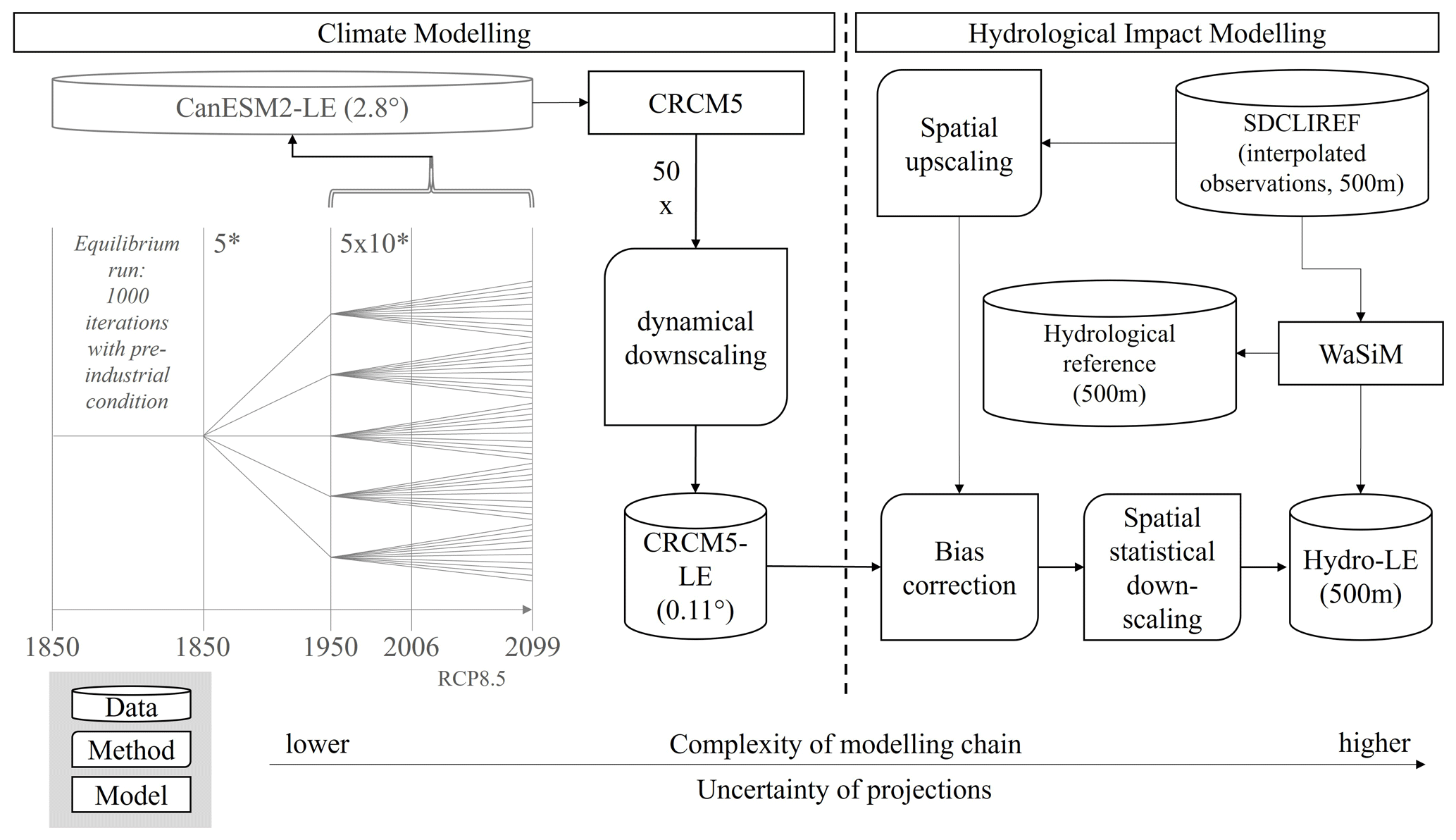
Figure 2 The ClimEx modeling chain uses the CanESM2 large ensemble (LE, gray, not created within the ClimEx project) to generate the CRCM5-LE. The CRCM5-LE is then used to explore the impacts of climate change on the hydrology of hydrological Bavaria through a hydrological large ensemble (hydro-LE) created using the hydrological model WaSiM. The SDCLIREF dataset of interpolated meteorological observations was employed to calibrate and validate the hydrological model, as well as for the bias correction. The CRCM5-LE represents a SMILE, consisting of a single model that downscales output from the employed ESM using slight differences in the initialization.

Since the introduced model chain requires a vast number of computational resources, the ClimEx project employed the high-performance computing systems of the Leibniz Supercomputing Centre (LRZ), as well as its technical and consultative support to migrate and adapt software and data to its systems, to facilitate calculations, and to provide an extensive amount of storage to archive the data and make them available to the scientific community (data available at https://www.climex-project.org).

2.2.1 Climate data

A SMILE composed of 50 independent members of the Canadian Earth System Model version 2 (CanESM2) large ensemble (LE) was used as a base for all further analysis. The CanESM2-LE was produced by the Canadian Centre for Climate Modeling and Analysis (CCCma) and has been described in previous publications (Fyfe et al., 2017; Kirchmeier-Young et al., 2017; Arora et al., 2011; Leduc et al., 2019). All members of the CanESM2-LE used natural and anthropogenic forcings for the historical period from 1950 to 2005 and the representative concentration pathway 8.5 (RCP8.5; van Vuuren et al., 2011) emission scenario from 2006 to 2099 (Kirchmeier-Young et al., 2017; Leduc et al., 2019; Fyfe et al., 2017; Sigmond et al., 2018). The individual members differ only in terms of their initial conditions rather than in terms of changes in model structure, physics, or parameters; therefore, they offer a range of internal or natural variability of the climate system at a global scale.

These 50 members were dynamically downscaled from ∼ 2.85° (≈ 310 km) to 0.11° (≈ 12 km) using the Canadian Regional Climate Model version 5 (CRCM5; Martynov et al., 2013; Šeparoviæ et al., 2013) over two spatial domains, the European and the northeastern North American domains (Leduc et al., 2019). As with the CanESM2-LE, variations between the individual members were obtained by unique initial conditions for each member, thus providing a range of internal or natural variability on a regional scale. The resulting CRCM5 large ensemble (CRCM5-LE; Leduc et al., 2019) of 50 transient members provides the basis for assessing the impact of climate change on hydro-meteorological extreme events for hydrological Bavaria. We focus on the model years 1961 to 2099 as opposed to 1950 to 2099 to account for the time it takes for the RCM to produce fully independent realizations due to the inertia of the ocean model (Leduc et al., 2019). A comparison between the CRCM5-LE and the E-OBS observational gridded dataset (Haylock et al., 2008) on the CRCM5 grid revealed biases for a historical period between 1980 and 2012, showing regional and seasonal variations in the magnitude of temperature and precipitation over Europe (Leduc et al., 2019). Since the creation of RCM-LEs is challenging in terms of computational demand (performance and storage), only a few are available to date (Addor and Fischer, 2015; Leduc et al., 2019; Aalbers et al., 2018; Brönnimann et al., 2018). However, all of the RCM-LEs differ in terms of their domain size, spatial resolution, and ensemble size. All RCM-LEs are ensembles of opportunity and are dependent on the availability of the driving GCM-LEs, which, in the CMIP5 phase, are all based on RCP8.5. Thus, in this study, only a single RCM-LE, as well as a single scenario, was employed.

Since this bias was considered to affect the behavior of the outputs of the hydrological model due to shifts in seasonality and magnitude, a bias correction was applied. The required meteorological data of precipitation, air temperature, relative air humidity, incoming shortwave radiation, and wind speed were adjusted to match a meteorological reference of interpolated 3-hourly station data (Sub-Daily Climate REFerence, SDCLIREF; Ludwig et al., 2019) on the RCM grid using an adaptation of the quantile-mapping approach of Mpelasoka and Chiew (2009). This approach, as described in Willkofer et al. (2018), involved using multiplicative or additive correction factors and was further adapted for using 3-hourly correction factors for every quantile and month (for further details, see Sect. S3 in the Supplement). To preserve an internal spread between the members, a single set of factors was deduced from a combination of all 50 members. Despite the numerous benefits (increased reliability of climate change projections of the hydrological impact model, reduced bias in mean annual discharge) and shortcomings (disrupting feedbacks between fluxes, modification of change signals, assumption of a stationary bias) of bias correction (e.g., Teutschbein and Seibert, 2012; Maraun, 2016; Ehret et al., 2012; Dettinger et al., 2004; Chen et al., 2021; Huang et al., 2014), bias correction is often inevitable for climate change impact studies (Gampe et al., 2019).

Subsequently, the bias-corrected data were statistically downscaled to the hydrological model scale (500 m × 500 m) using a mass-preserving approach (Marke, 2008; Ludwig et al., 2019). This approach involved the spatial interpolation (inverse distance weighting) of anomalies for each time step from the monthly mean reference state (1981–2010) at the CRCM5-LE cell center points to the hydrological model scale (Brunner et al., 2021b). The interpolated time step anomalies at the hydrological scale were then applied (multiplied or added) to the respective gridded monthly climatological reference fields of the SDCLIREF (Brunner et al., 2021b). In order to ensure the mass conservation, the downscaled RCM data were upscaled to the original RCM grid scale (mass conservative remapping) and compared to the RCM time step values to determine any correction factors necessary, which were then applied to the downscaled grid cells to close the mass balance.

For further details, readers are referred to a comprehensive summary in the Supplement for the CanESM2-LE (Sect. S1), the CRCM5-LE (Sect. S2), and the bias correction (Sect. S3).

2.2.2 Hydrological model WaSiM

The Water balance Simulation Model (WaSiM; Schulla, 2021) was employed to perform the hydrological simulations driven by the CRCM5-LE, resulting in a hydro-SMILE (the WaSiM-LE). WaSiM is a distributed, mostly physically based, and deterministic model for simulations on various spatial (1 m to 10 km) and temporal (minute to daily) scales, with a constant time step. It includes routines for evapotranspiration, snow accumulation and snowmelt, glaciers, soil water transfer, groundwater, and discharge generation and routing (Schulla, 2021). The model is frequently used for hydrological climate change impact studies on various topics, such as glaciers, groundwater, and discharge, for small-scale to mesoscale catchments (Iacob et al., 2017; Neukum and Azzam, 2012; Jónsdóttir, 2008).

The model was set up at a high spatiotemporal resolution (500 m and 3 h) for 98 catchments of hydrological Bavaria, with a focus on high-flow representation using distributed data derived from the European DEM (EU-DEM; European Environment Agency, 2013), land use data provided by the CORINE land cover dataset (European Environment Agency, 2019), distributed soil information from the European Soil Database (ESDBv2.0; Panagos, 2006; European Commission and the European Soil Bureau Network, 2004), and groundwater information provided by the Hydrogeologische Übersichtskarte (HÜK; Dörhöfer et al., 2001) and International Hydrogeological Map of Europe (IHME; BGR, 2014). A single set of parameters for spatially distributed modules (i.e., evapotranspiration, soil properties) was defined globally for the entire modeling domain (Willkofer et al., 2020). Although there are abundant in situ data available for the study region, these are mainly provided as point measurements which are often representative of the entire catchment area and therefore require interpolation to the hydrological model resolution, which can introduce large uncertainties. Furthermore, some approaches of the hydrological model offer free parameters which cannot be measured. Hence, a calibration of the model for a limited number of free and usually locally measurable parameters was deemed to be necessary. For further details about the model calibration procedure, we would like to refer to Willkofer et al. (2020). Local parameters for discharge storage components (i.e., interflow, direct flow) were calibrated using an automated algorithm (dynamically dimensioned search (Tolson and Shoemaker, 2007) and simulated annealing with progressing iterations (Černý, 1985; Kirkpatrick et al., 1983)), minimizing a weighted combination of performance metrics (overall metric – OM; Eq. 1), including the Nash–Sutcliffe efficiency (NSE; Nash and Sutcliffe, 1970), the Kling–Gupta efficiency (KGE; Gupta et al., 2009), the logarithmic NSE, and the ratio of root mean squared error to standard deviation (RSR; Moriasi et al., 2007; Willkofer et al., 2020). A best fit would result in OM = 0, with larger deviations from 0 indicating a worse model fit. Due to the focus on high-flow representation, more emphasis was placed on the respective measures (i.e., NSE and KGE). For further details about the model setup, the reader is referred to Willkofer et al. (2020).

$$\begin{array}{}\text{(1)}& \begin{array}{rl}\mathrm{OM}& =\mathrm{0.5}\times \left(\mathrm{1}-\mathrm{NSE}\right)+\mathrm{0.25}\times \left(\mathrm{1}-\mathrm{KGE}\right)\\ & +\mathrm{0.15}\times \left(\mathrm{1}-\log \mathrm{NSE}\right)+\mathrm{0.1}\times \mathrm{RSR}\end{array}\end{array}$$

The simulations of a single parameter set for various catchments within a heterogeneous landscape revealed satisfactory to very good results for most of the 98 gauges during the 30-year reference period of 1981 to 2010. However, for a few gauges, the model was not able to reproduce the observed discharge satisfactorily (16 (5) gauges showing NSE (KGE) values below 0.5; see also Fig. S1a and b in Sect. S4 in the Supplement) (Willkofer et al., 2020; Poschlod et al., 2020). Furthermore, the simulations reproduced the mean high flow sufficiently well, with over 60 % of the gauges showing absolute deviations from observed values below 20 %. Nonetheless, gauges in alpine or pre-alpine catchments exhibited a deficit in mean high-flow values due to the lack of observed precipitation resulting from an undercatch of precipitation for that region (Poschlod et al., 2020). Consequently, the level of trust (LOT) for the peak flows of flood events with return periods of 5, 10, and 20 years, introduced in Willkofer et al. (2020), showed a moderate to high confidence for most catchments. The LOT further depends on the model performance to a certain degree, where gauges depicting a lower model performance often exhibit a lower LOT as well. LOT values were not provided for extreme flood events (i.e., 100-year flood events) since they are subject to significant epistemic uncertainty due to the restricted availability of simulated data (30 years). In Brunner et al. (2021a), the same hydrological model simulations were evaluated on a daily timescale – in contrast to the 3-hourly timescale used here – in terms of general evaluation metrics (i.e., NSE, KGE, volume efficiency, and mean absolute error), as well as for flood-specific characteristics (i.e., number of events, mean timing of the event, mean volume, mean duration). The evaluation of flood characteristics showed a good agreement on the number of events, showing only a slight underestimation of events; a good agreement on the timing of events, with only a slight delay in flood occurrence; and an overestimation of flood volume and duration.

Due to the holistic calibration approach employing a single set of parameters over several heterogeneous catchments, the at times poor performance of individual catchments can be expected as catchment-specific characteristics can only be considered to a certain extent (e.g., karstic soils, transfer systems, artificial reservoirs). While calibrating each catchment individually might lead to a higher performance at the respective catchment scale, it also increases the likelihood of overfitting. Furthermore, since the hydrological model serves climate change impact analysis, relative change values are of more interest than changes in absolute values. Nonetheless, the performance must be considered for interpretation. A brief overview of the model's performance for each gauge is given in the Supplement (Sect. S4).

The resulting hydro-SMILE comprises 50 members of transient simulated data from 1961 to 2099, providing a total of 6950 model years to be exploited to analyze extreme values.

2.2.3 Benefit of a hydro-SMILE for the estimation of extreme peak flows

This study used the simulated discharge for the reference period of 1981 to 2010, taken out of the entire dataset, to assess the benefits of the hydro-SMILE in estimating return levels. Like the individual members of the CRCM5-LE, the members of the WaSiM-LE are equally probable and, therefore, provide a comprehensive database to facilitate the analysis of extreme values.

Figure 3 Process chain illustrating the benefit of a hydro-SMILE for climate change impact studies on peak flows of extreme return periods. The process includes extreme value analysis (EVA) based on annual maximum (AM), with bootstrapping resampling to create n different samples of sample size m. The probability of non-exceedance (p) and the generalized extreme value (GEV) distribution with the L-moment (LM) estimators are used to derive estimates for high-flow values of the return period T (HF_T) for the samples (m), all data (1500), and the benchmark (BM). The statistical analysis was performed using the extRemes package (v2.0) for R (Gilleland and Katz, 2016).

Figure 3 illustrates the approach taken to emphasize the benefits of the hydro-SMILE in analyzing peak flows of high return periods for the reference period. The 30-year reference period (ref) was selected for all 50 members, resulting in 1500 model years (50 members × 30 years) of discharge data for each of the 98 gauges. First, the annual maximum of each model year (hydrological year) was extracted for the analysis. Since the database consists of 1500 model years, this number is considered to be sufficient to employ empirical non-exceedance probabilities (Martel et al., 2020). However, to demonstrate the benefit of the hydro-SMILE database a statistical analysis using the stationary GEV distribution was also conducted for comparison purposes. A bootstrapping approach with resampling was used to create 1000 samples (n) of different sizes m (30, 100, and 200 years) (each sample without replacement). Using 1000 samples ensures that one value of the 1500 AM has a chance of > 99 % of being selected by chance for m = 30. The GEV was employed to estimate the return periods and corresponding confidence intervals. The parameters of the GEV distribution were estimated using L-moments (LMs). The GEV distribution was selected as it is among the better-performing methods relying on AM (Bezak et al., 2014) and is the recommended choice for German gauges (Salinas et al., 2014; Fischer and Schumann, 2016).

Although the sample size of 30 and 100 AM may be small for estimating peak flows of high return periods, they were selected along with a size of 200 AM as they represent an average (30 years) to rare (100 and 200 years) data availability of observed discharge values at different gauges (GRDC, 2021). The resulting 1000 estimates for return levels of peak flows offer a comprehensive database to demonstrate the benefit of the hydro-SMILE. Additionally, the GEV was calculated using the entire 1500-AM database for each gauge to allow for a comparison with a benchmark value. This benchmark for the return levels of peak discharge was deduced by applying the quantile based on the empirical probability of non-exceedance p (Eq. 2) to all 1500 AM values for each gauge, and it is considered to represent a robust estimate. This analysis focused on the 100-year flood, which is an event of the 100-year return period T (HF₁₀₀; T = 100), and the corresponding 99th percentile p of the distribution of the 1500 AM values as a benchmark.

$$\begin{array}{}\text{(2)}& p=\mathrm{1}-{\displaystyle \frac{\mathrm{1}}{T}}\end{array}$$

Values for the benchmark derived by the empirical probability, as well as the HF₁₀₀ values estimated using the GEV, are further normalized to the benchmark to allow for a better comparison.

2.2.4 Projection of changes in frequency and magnitude

This study further investigates the dynamics of the magnitude and frequency of HF₁₀₀ for three future periods (near future: 2020–2049, mid-future: 2040–2069, far future: 2070–2099) frequently used in similar CCI studies (e.g., Hattermann et al., 2018), providing the same database of 1500 AM values as for the benefit analysis. Therefore, the robust estimates of extreme return levels of peak flows derived by the empirical probabilities are used for the assessment of climate change impacts on their magnitude (C_M, Eq. 3) and frequency (C_F, Eq. 4a to c) in the three future periods.

$$\begin{array}{}\text{(3)}& C_{\mathrm{M}}=\left({\displaystyle \frac{{\mathrm{HF}}_{T_{\mathrm{fut}}}-{\mathrm{HF}}_{T_{\mathrm{ref}}}}{{\mathrm{HF}}_{T_{\mathrm{ref}}}}}\right)\times \mathrm{100}\mathit{\%}\end{array}$$

$$\begin{array}{}\text{(4a)}& {\displaystyle }{C}_{\mathrm{F}}={\displaystyle \frac{\mathrm{1}}{\mathrm{1}-f\left({\mathrm{HF}}_{T_{\mathrm{ref}}}\right)}}\text{(4b)}& {\displaystyle }f=F\left({\mathrm{HF}}_{T_{\mathrm{fut}}}\right)\text{(4c)}& {\displaystyle }F\left(x\right)={\sum }_{i=\mathrm{1}}^j{h}_i={\sum }_{i=\mathrm{1}}^j{\displaystyle \frac{h\left(x_i\right)}{n}}\end{array}$$

The change in magnitude is given as the difference between the future (HF${}_{T_{\mathrm{fut}}}$) and reference value (HF${}_{T_{\mathrm{ref}}}$) relative to the reference value in percent. The change in frequency is expressed as the return period value T and is calculated by applying the empirical cumulative distribution function F (with a frequency for an event h_i described as the ratio between the frequency for the specific event h_(xi) and the number of all values n, Eq. 4c) for the respective future period (f, Eq. 4b) to the value of the 100-year flood of the reference period (Eq. 4a). The quantile value of f for the reference 100-year flood value is then used to deduce the future return period by solving the empirical probability of non-exceedance for the return period T (Eq. 4a). The change signals are calculated for each of the above-mentioned 30-year future periods. However, this analysis requires stationarity for the underlying data. Since we use all the 1500 model years provided by the 50 members, we determine stationarity if fewer than 5 % of the members exhibit a significant trend for each individual gauge. A Mann–Kendall (MK) test (Mann, 1945; Kendall, 1955) for stationarity conducted on each individual member and gauge revealed no significant trend for the reference period (with significance level α = 0.01) for more than 95 % of the members along all gauges. However, for the future periods, the MK test exhibits significant trends for more than 5 % of the members in 6 of the 98 gauges. Limiting the evaluation periods to 20 years instead of 30 years lead to similar results for the MK test, showing no apparent trend for all gauges in the reference period but showing a significant trend (more than 5 % of members with a trend) for at least one gauge in the future periods. Poschlod et al. (2020) and Brunner et al. (2021b) conducted their analysis on the same database using time slices of at least 30 years as well. Thus, we choose to use 30-year periods since stationarity criteria are met in most catchments, and we opt for the larger database, as well as maintaining consistency with these studies.

2.2.5 Dynamics of driving mechanisms

The employed process-based hydrological model allows for a more detailed investigation of the dynamics of the driving mechanisms of extreme discharges of the 100-year flood and beyond. First, extreme events of magnitudes of at least HF₁₀₀ are extracted for each of the 98 gauges and 50 members of the hydro-LE. To avoid sampling a single event multiple times, a 5 d period was used to separate individual events, as suggested by Svensson et al. (2005). The starting date of the events served as entry to extract data from potential flood drivers, which include precipitation, melt from snow and glaciers, and soil water content prior to the event. Precipitation events were further separated into heavy-rain events (hr) and steady-rain events (sr), while there was no distinction between liquid and solid precipitation. The respective thresholds to identify and separate the different precipitation event types (see Table 1) were adopted from the German Weather Service (DWD, Deutscher Wetterdienst, 2024).

Table 1 Thresholds for the identification of the driving mechanisms (drivers) of extreme-discharge events above HF₁₀₀. P represents the precipitation events of heavy rain (hr) and steady rain (sr), melt represents melting water from snow and glaciers (in mm snow water equivalent), and SWC_root represents the soil water content of the soil's root zone.

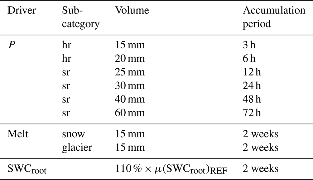
Table 2 Composition of the different drivers for the analysis of the dynamics of the HF₁₀₀ driving mechanisms.

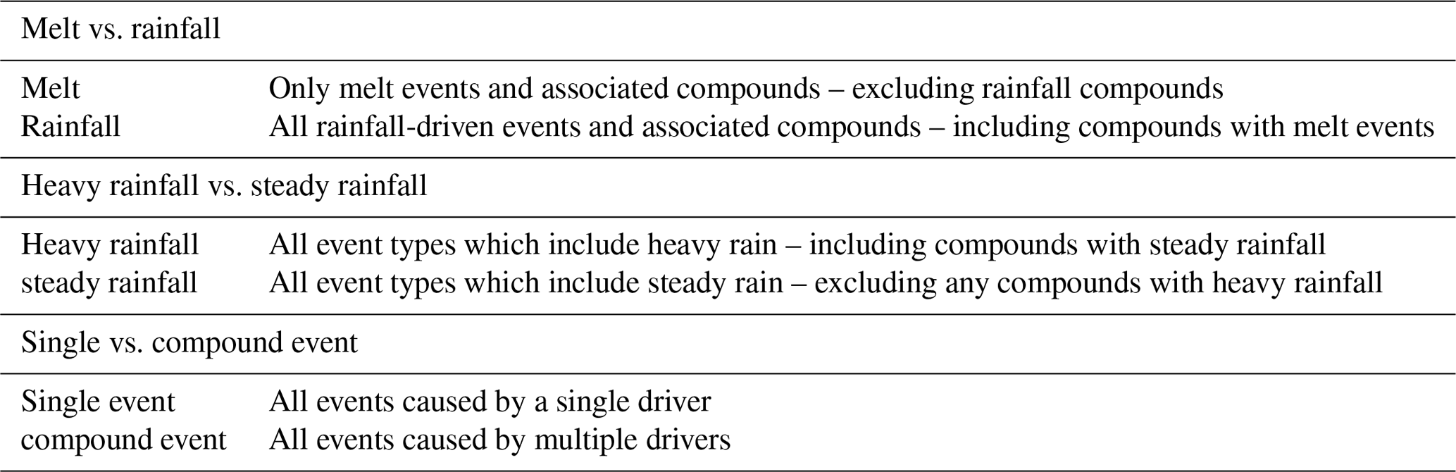
A melt-driven event (snow and/or glacier) was identified if the snow water equivalent from melt exceeded 15 mm 2 weeks before the event (adapted from Brunner et al., 2021b). Extreme-discharge events may also be caused by a superposition of these driving mechanisms and are often referred to as compound events (e.g., rain on snow, rain on saturated soils). Thus, if more than one driver is identified, we ascribe it to the compound event type. Furthermore, since an elevated soil water content cannot be responsible for an extreme-discharge event alone, it is only considered to be a contributing factor and is always part of the compound event type. In this case, the contribution of an elevated soil water content is considered when the soil water content is 10 % higher than the long-term mean soil water content for the entire reference period. All possible combinations (single drivers and compound events) result in 32 different or superimposed mechanisms. To reduce complexity and to focus on specific aspects of the different drivers, we aggregate the 32 possible combinations to six different major contributions listed in Table 2.

First, we analyze the dynamics of melt vs. rainfall events; second, the dynamics of heavy rainfall (convective events) vs. steady rainfall (advective events) are investigated; and third, we illustrate the dynamics of single drivers (any type) vs. compound events (any type).

3 Results

3.1 Benefits of hydro-SMILEs for the estimation of extreme return periods of peak flows

Large ensembles provide a vast amount of data; therefore, they are considered to be beneficial for extreme value analysis (Kendon et al., 2008; Kjellström et al., 2013; Wood and Ludwig, 2020). The benefit of a hydro-SMILE in determining robust extreme hydrological discharge values for hydrological Bavaria is analyzed, specifically for the 100-year flood. The robust values for the discharge gauges, derived using the empirical probability of non-exceedance for a 100-year event, serve as a benchmark for comparison with values derived by the GEV distribution using three different sample sizes (30, 100, 200) of AM values (Fig. 4).

Figure 4 Comparison of HF₁₀₀ estimates calculated using the GEV distribution with 1000 AM samples of (a) 30, (b) 100, and (c) 200 years per gauge (blue markers) with the respective benchmark value (solid black line) for 98 gauges.

Table 3 Summary of overall statistics of the relative deviation of the HF₁₀₀ estimates from the benchmark value across all gauges. The table includes the number of samples (n), the sample size (m) given in annual maximum (AM) values, and the 0.25 and 0.75 quantile (Q25, Q75) values.

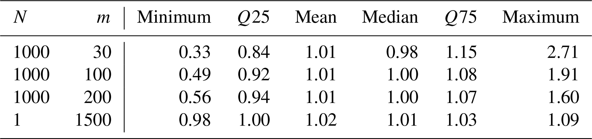
The results shown in Fig. 4a, b, and c illustrate that the estimates of HF₁₀₀ are more robust with an increasing number of AM values used for the GEV, as indicated by the decreasing spread of the blue markers around the black benchmark line with increasing sample size. Table 3 summarizes the statistical characteristics of the deviation of the estimates from the benchmark across all 98 gauges. While the range of the relative deviation of the 1000 samples of HF₁₀₀ estimates from the benchmark is between 0.33 and 2.71 when calculated with a sample size of 30 AM values (Fig. 4a), this range diminishes to 0.49 and 1.91 for 100 AM values (Fig. 4b) and 0.56 and 1.60 for 200 AM values (Fig. 4c). Therefore, the range of the 1000 estimates diminishes with an increase in sample size, and the values cluster more densely around the benchmark. However, despite the remaining non-negligible range of deviations from the benchmark, the mean (1.01) and the median (0.98 to 1.0) across all values for all gauges are close to the benchmark value for different sample sizes. The inner 50 % of the 1000 samples across all 98 gauges exhibits the largest deviation with a sample size of 30 AM (between 0.84 and 1.15) and the lowest deviation for 200 AM (0.94 to 1.07). Therefore, only 25 % of the samples show underestimations below 0.84 (0.92, 0.94), and only 75 % exhibit overestimations larger than 1.15 (1.08, 1.07) with a sample size of 30 AM (100 AM, 200 AM). Thus, with deviations larger than 15 % for 50 % of the estimates calculated using a sample size of 30 AM, only half of the estimated HF₁₀₀ values are within an acceptable range (±15 %, considering model parameter uncertainty and errors in observations affecting the model quality regarding high flows) compared to the benchmark. This number increases with a larger sample size.

While the majority of gauges show estimates that are evenly distributed around the benchmark, some gauges exhibit a tendency towards over- or underestimation of the HF₁₀₀ estimates, with more values falling above or below the benchmark line. This behavior may be different when using more than 1000 samples to conduct the analysis. The difference between the benchmark value obtained from empirical probability and the estimates obtained from the GEV distribution can vary greatly depending on the samples selected from 1500 AM values.

A comparison between the HF₁₀₀ estimates derived using the empirical probability of non-exceedance and those obtained using the GEV distribution is shown in the Supplement (Sect. S5). The values gained from the GEV distribution still exhibit deviations from the benchmark, although they are only marginally different from it.

3.2 Changing dynamics of the 100-year peak flows in future projections

The changes in HF₁₀₀ for the investigated gauges in hydrological Bavaria in the 21st century are summarized for five distinct discharge regimes (defined by the Pardé coefficient) which were adapted from Poschlod et al. (2020) (Fig. 1). The regimes comprise the glacio-nival regime of four high-alpine catchments, a nival regime of mostly alpine to pre-alpine catchments, a nivo-pluvial regime of pre-alpine catchments, a balanced pluvial regime (little variation in mean monthly discharges) along the Danube and its tributaries in the Alpine Foreland, and the unbalanced pluvial regime (more pronounced peak in monthly discharge from January to March) (Poschlod et al., 2020). One gauge that was originally assigned to its own regime in Poschlod et al. (2020) has been re-allocated to the pluvial (unbalanced) regime as it exhibits a similar mean discharge behavior.

Within the study area, the flood protection structures are typically designed based on a stipulated estimation of HF₁₀₀ from observations, which represent a stationary condition in the past. Any future increase in the magnitude and frequency of these extreme values poses a threat to these structures.

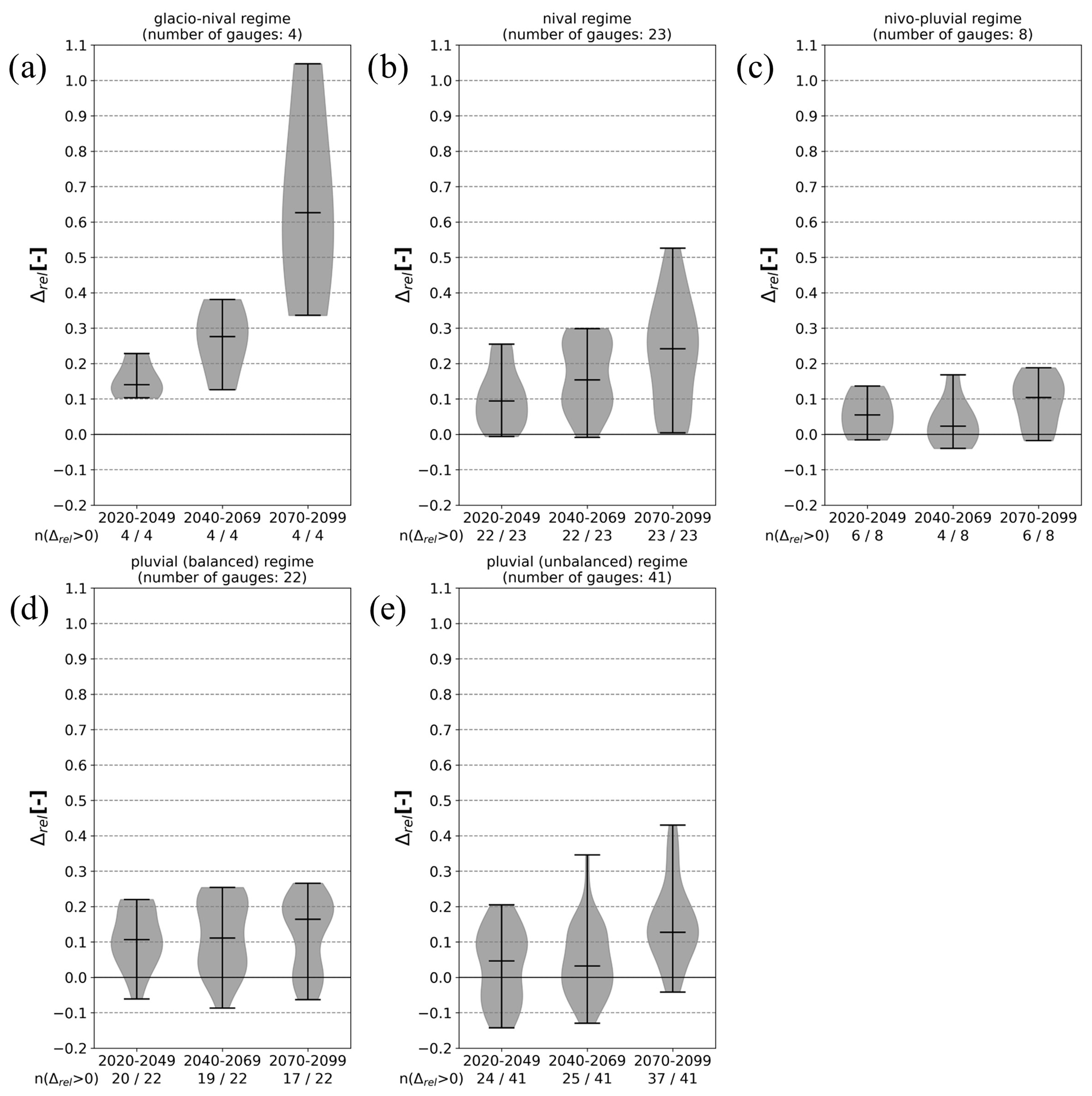
Figure 5 Violin plots indicating the changes in the magnitude of HF₁₀₀ for the three future periods (near, middle, far) compared to the reference period, with changes presented as the relative difference (Λ_rel) between the reference and the future HF₁₀₀ value for each gauge. Results of the 98 gauges are aggregated for the five discharge regimes: (a) glacio-nival, (b) nival, (c) nivo-pluvial, (d) pluvial (balanced), and (e) pluvial (unbalanced). The figures display the total number of gauges per regime, as well as the number of gauges depicting an increase in magnitude.

Figure 5 displays violin plots that illustrate the range of changes in the magnitude of HF₁₀₀ events for the different discharge regimes, as well as the distribution of changes across the respective clusters of gauges for the near- (horizon 2035), mid- (horizon 2055), and far-future (horizon 2085) periods. Overall, 78 % of all gauges ($\mathrm{76}/\mathrm{98}$) show an increase in magnitude for the 2035 horizon, 76 % ($\mathrm{74}/\mathrm{98}$) show an increase in magnitude for the 2055 horizon, and 89 % ($\mathrm{87}/\mathrm{98}$) show an increase in magnitude for the 2085 horizon.

The CCI values are most severe for the glacio-nival regime (Fig. 6a) as all three future periods exhibit an increase in the magnitude of the HF₁₀₀ events of at least 10 % compared to the reference period. The nivo-pluvial regime (Fig. 6c) shows the smallest spread and the lowest increase in HF₁₀₀ magnitude across all future periods compared to the reference period. As the distance from the Alps increases and the discharge regimes shift from snowmelt influenced to more precipitation driven, the number of gauges projecting a decrease in HF₁₀₀ intensities increases. However, the majority of gauges still exhibit an increase in intensities, with up to 18.8 % for the nivo-pluvial regime (Fig. 5c), 26.6 % for the balanced pluvial regime (Fig. 5d), and 43 % for the unbalanced pluvial regime (Fig. 5e) in the far future. The gradient of an increase in magnitude over all three projection periods is small for the nivo-pluvial and balanced pluvial regimes, which show the least intensification in terms of HF₁₀₀ values for the respective periods. However, the gradient of increase is more distinct for the remaining regimes, with the largest increase in the glacio-nival regime (Fig. 5a). The gauges in this regime depict the strongest increase in HF₁₀₀ intensities for the 2085 horizon, with an increase of 36.6 % to 104.7 %.

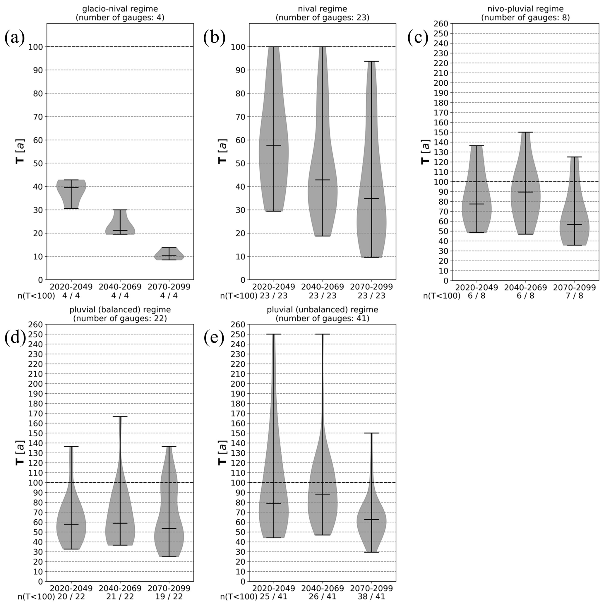
Figure 6 Violin plots indicating the changes in the frequency of HF₁₀₀ for the three future periods (near, middle, far) compared to the reference period, with changes presented as absolute values of return periods (T[a]) of the respective future period compared to the 100-year return period for each gauge. Results of the 98 gauges are aggregated for the five discharge regimes: (a) glacio-nival, (b) nival, (c) nivo-pluvial, (d) pluvial (balanced), and (e) pluvial (unbalanced). The figures display the total number of gauges per regime, as well as the number of gauges depicting an increased frequency.

Based on the future projections of the hydro-SMILE, the discharge values of HF₁₀₀ are likely to increase for most of the gauges of hydrological Bavaria. Consequently, the frequency of the HF₁₀₀ discharge for the reference period also increases. Figure 6 shows the change in frequency between the future and the reference period for the different regimes.

Values indicate the new return period associated with the HF₁₀₀ discharge from the reference period. This means values below 100 indicate an increase in frequency. The glacio-nival regime (Fig. 6a) also exhibits the strongest increase in frequency among all regimes, with HF₁₀₀ of the past becoming equivalent to a 31- to 43-year event in the near future, thus becoming roughly 2 to 3 times more frequent. For the 2085 horizon, the same HF₁₀₀ event becomes an 8- to 14-year event, showing a 7- to 12-fold increase in frequency. A similar development is visible for some gauges in the nival regime (Fig. 6b). While the violin plot for this regime indicates that the reference 100-year event will become a 70-year event for more than 50 % of gauges, some gauges show no or only a minor increase in frequency as well. The changes for the remaining regimes are less severe but still indicate an increase in frequency for up to 50 % of the respective gauges until the middle of the century and for more than 50 % in the far future. The changes for the nivo-pluvial regime (Fig. 6c) and the unbalanced pluvial (Fig. 6d) regime show that the frequency declines for less than 50 % of the gauges in the near- and mid-future periods. Therefore, the 100-year event becomes more frequent for more than 50 % of the gauges with varying extent. While the magnitude of changes is similarly moderate (except for the far future) for Fig. 6c and e, projected future return periods for the HF₁₀₀ event for Fig. 6d depict stronger change signals towards higher frequencies with more than 50 % of gauges showing values smaller than 60 years. Furthermore, the nivo-pluvial, as well as the balanced and unbalanced pluvial regimes, exhibits a slight decrease in frequency in the middle future compared to the remaining projection periods, while the magnitude does not show this behavior. However, this circumstance may be explained by the change in the driving agent from snowmelt-driven events in the near future to rainfall-induced events at the end of the century. Thus, at the 2055 horizon, the shift in the ratio of both event types contributes to this slight decline in frequency.

Some gauges within the nivo-pluvial and both pluvial regimes depict an, in part, large decrease in frequency and/or magnitude. These gauges usually exhibit natural or artificial influences, such as the retention effect of natural lakes, reservoirs, or diversions or gauges of small catchments which might experience fewer dynamics in the changing of flood drivers or even a reduction.

Overall, the changes in frequency and magnitude due to the projected changes in climate according to the CRCM5-LE become less severe with increasing distance from the Alps. Furthermore, the increase in frequency and magnitude for alpine catchments is seemingly high but is in line with the results of Hattermann et al. (2018), which showed comparable results for the near-future period (100-year event frequency between 20 and 40 years). The influencing factors for these sometimes severe changes are manifold. However, Brunner et al. (2021b) analyzed the relation between the extremeness of precipitation and discharge for 78 out of the 98 gauges within hydrological Bavaria and concluded that an increase in extreme-precipitation magnitude is of higher importance for extreme return levels of discharge than land surface processes, such as antecedent soil moisture or changes in snowpack due to warmer temperatures. If precipitation volumes are sufficiently large, they quickly saturate the soil or yield an excessive amount of direct runoff due to infiltration excess (Brunner et al., 2021b).

The mean magnitude of the annual maximum precipitation is projected to change for different temporal aggregation levels (3-hourly to 5-daily) in the CRCM5-LE (Wood and Ludwig, 2020); in addition, the magnitude of the 100-year return period rainfall increases by 10 %–20 %, and the frequency increases by 2 to 4 times (Martel et al., 2020) for hydrological Bavaria. The changes are associated with seasonal shifts from summer to winter events and are particularly pronounced in the alpine region (Martel et al., 2020; Wood and Ludwig, 2020). Severe floods that occur simultaneously in different catchments of the study area are usually associated with a cutoff-low Vb cyclone that results in prolonged precipitation events lasting up to 15 d over the same region (Stahl and Hofstätter, 2018; Mittermeier et al., 2019). Under the changing climate conditions projected by the CRCM5-LE by the end of the 21st century employing the RCP8.5 scenario, these events are likely to intensify in volume and frequency during winter and spring and are likely to occur less frequently during the summer months but with an increased precipitation volume (Mittermeier et al., 2019).

The spatial distribution of the dynamics in HF₁₀₀ frequency and magnitude is shown in the Supplement (Sect. S6).

3.3 Changes in driving mechanisms

Figure 7 shows the dynamics of three different combinations of driving mechanisms (columns of panels) listed in Table 1 for extreme-discharge events equal to and above HF₁₀₀ between the reference period (REF) and the three future periods (FUT1 to FUT3) for the five different discharge regime types (rows of panels). As mentioned in the “Data and methods” section, the 32 possible combinations were aggregated to six groups, as listed in Table 2.

Figure 7 Dynamics in driving mechanisms of floods equal to or larger than HF₁₀₀ for the five different discharge regimes and within the four different periods. The columns of panels show the composition of melt- vs. rainfall-driven events (left), heavy-rainfall vs. steady-rainfall events (center), and single vs. compound events (right). The rows of panels correspond to the five different discharge regimes, as indicated by the regime type on the right y axis. The bars in each individual panel show the cumulative ratio of the different mechanisms for the reference period (REF, 1981–2010) in the first bar, and the following bars represent the different future periods (FUT1: 2021–2040; FUT2: 2041–2070; FUT3: 2070–2099).

The first column of panels in Fig. 7 shows the changes in the ratio between snowmelt-driven events (excluding rainfall compounds) and rainfall-driven events (including melt compounds). Figure 7f–j show the changes in the ratio between heavy-rainfall and steady-rain events (excluding snowmelt events from Fig. 7a–e), and Fig. 7k–o depict the changes in the ratio of events that can be attributed to a single cause and to a compound of drivers.

The glacio-nival and the nival regimes show the highest ratio of snowmelt-driven events (Fig. 7a and b). For the reference period, this event type is the major driver for the extreme discharges for the glacio-nival regime (67.7 %), while, for all other regimes and periods, rainfall and its compounds dominate the ratio. Figure 7a to e also show a seventh category of “other”, which, in this case, comprises events which could not be ascribed to any of the investigated drivers and are likely events that originate from an upstream flood. All regimes indicate a decrease in snowmelt-driven event types form the REF period to the far-future (FUT3) period, with the largest decrease being visible for the glacio-nival regime (67.7 % to 20.6 %). In the nivo-pluvial and pluvial regimes (Fig. 7c to e), the ratio of snowmelt event types becomes negligible in the future, with values of only slightly above 0 %. Furthermore, the ratio of snowmelt events diminishes from the glacio-nival and nival regime to the pluvial regimes (Fig. 7c to e) with increasing distance to the Alps. The pluvial regimes (Fig. 7d and e) show only minor changes in the ratio of rainfall events from REF to FUT3 (89.3 % to 80.6 % for the unbalanced regime and 84.6 % to 87.5 % for the balanced regime). The disappearance of snowmelt-driven events in future periods indicates that more events are driven factors falling in the category of other, with an increase in this category being seen especially in the nival regime (3.2 % to 10.1 %) and the unbalanced pluvial regime (9.2 % to 18.9 %). Overall, these results indicate a reduction in snow accumulation during the winter due to an increase in winterly temperatures of between 3 and 5 °C, as projected by the driving CRCM5-LE for the end of the century (FUT3) for middle Europe (von Trentini et al., 2020). For the glacio-nival and nival regimes, the large decrease in the snowmelt ratio also indicates a reduced contribution of melt from glaciers due to severe loss of mass towards the far future.

Figure 7f–j illustrate the dynamics in the ratio of hr and sr event types, therefore representing only the rainfall part of Fig. 7a to e. In all five regime types, the hr event type and its compounds (including compounds with sr) are the dominant driver, with a ratio of 58.8 % in the pluvial unbalanced regime (REF) to 88.4 % in the glacio-nival regime (FUT3). The percentage of hr events increases towards the end of the century for all regimes by 4 (pluvial balanced) to 17.2 (pluvial unbalanced) percent points, except for the pluvio-nival regime, where the percentages first increase from REF in FUT1 (88.9 %) and FUT2 (89.2 %) and then decrease again for FUT3 to the level of REF (REF: 84.4 %, FUT3: 84.8 %). The glacio-nival and pluvial unbalanced regimes show the strongest increase in hr event types from REF to FUT3, with 14.7 and 17.2 percent points, respectively. The dynamics for these regimes may be caused by an increase in summer temperatures (between 5 and 6.5 °C) but also in spring and fall temperatures towards the end of the century, as projected by the CRCM5-LE (von Trentini et al., 2020). The higher temperatures result in more available water vapor and, thus, precipitable water in the atmosphere and a higher potential for convective (hr) events, especially over the Alps (Giorgi et al., 2016). Furthermore, the strong increase for the alpine gauges of the glacio-nival regime may be related to a stronger increase in heavy-precipitation events over the Alps compared to regimes outside the Alps (Wood and Ludwig, 2020). In general, the balanced and unbalanced pluvial regimes show the lowest contribution of hr events (59 % and 58.3 % in REF); therefore, any change in the number of hr events or a general increase in the intensity of short-duration rainfall might lead to more events being classified as hr compounds. On the other hand, in other regimes, the hr compound is already large, and, hence, any changes in the rainfall dynamics will only yield a limited increase in the event classification.

Figure 7k–o illustrate the dynamics in the ratio between single-driver event types and compound event types for the five different regimes. Here, the compound class comprises the snowmelt and rainfall event types in Fig. 7a–e, neglecting events classified as other. Therefore, single-driver event types depict events caused by only one of the driving mechanisms listed in Table 1, whereas compound event types comprise all other possible combinations. In all five regimes and time periods, compound drivers are attributed to at least 50.7 % (FUT3, pluvial unbalanced) and up to 82.9 % (FUT3, nivo-pluvial) of events. Except for the two pluvial regimes (balanced and unbalanced), there is very little change in the ratio. For these regimes, the number of events caused by a single driver increases form REF to FUT3 by 6 and 18.8 percent points for the balanced and unbalanced regimes, respectively. This strong signal in the dynamics for the unbalanced pluvial regime indicates an increase in short events of high intensity, which, in turn, may lead to a higher risk for flash floods. The nivo-pluvial regime further depicts a slight decrease of 8.8 percent points in events caused by a single driver from REF to FUT3.

4 Discussion

The variability of statistical characteristics within a time series can affect the estimation of extreme values due to extraordinary events (Fischer and Schumann, 2016). The results of this study emphasize the benefit of using data provided by a climatological SMILE for hydrological impact studies as this provides a profound basis for extreme value statistics and allows for more accurate estimation of extreme values, as also shown by other studies (van der Wiel et al., 2019; Champagne et al., 2020; Ehmele et al., 2020; Maher et al., 2021). In particular, van der Wiel et al. (2019) follow a similar approach for comparing statistical distributions and use an empirical approach to derive extreme-discharge values by employing a different approach for the creation of a 2000-year large ensemble of climate data forcing a global hydrological model. Our study shows similar results for the comparison between statistical estimates and empirically derived HF₁₀₀ values, favoring the empirical over the statistical approach when using a large ensemble of hydrological model data. However, the sometimes large deviations between the benchmark (robust estimate derived from the empirical probability for a 100-year flood event using 1500 AM values) and the estimates derived using a GEV based on different sample sizes (30, 100, 200) might be reduced when using an extreme value distribution (EVD), which is better suited to the respective sample when enough data are available (i.e., when using a hydro-SMILE, as shown here). In some cases, the GEV might not be the best distribution for the samples of the respective gauge, which might affect the differences from the benchmark since higher quantiles heavily depend on the distribution (Schulz and Bernhardt, 2016). Hence, a large ensemble of hydrological model data further reduces the uncertainties originating from different distributions, which may be considerable, as shown by Lawrence (2020). However, the approach presented in this study illustrates the benefit of a hydro-SMILE as it provides a more robust estimate by employing empirical probabilities for the deduction of extreme values. Therefore, these robust estimates allow for a more robust assessment of future dynamics of extremely high flows and their driving mechanisms, as also shown in Brunner et al. (2021b).

The results of this study are subject to uncertainties (parameters, process description) as they are produced by data created at the end of a cascade of modeling steps usually applied for climate change impact studies, as displayed in Fig. 2. Different components (e.g., climate model, hydrological model, bias correction) affect different discharge characteristics or indicators (e.g., extreme indicators, mean discharge) (Gampe et al., 2019; Muerth et al., 2012, 2013; Velázquez et al., 2013; Willkofer et al., 2018). A thorough assessment of the contribution of the chain compartments to the overall uncertainty would require an ensemble of multiple climate and hydrological models.

The overall strong increase in the frequency and magnitude of HF₁₀₀ in the future may be driven by deficiencies in the employed hydrological model, such as the generalized glacier model among affected catchments, or the single snowmelt approach used for the entirety of hydrological Bavaria (as described in Willkofer et al., 2020). However, as stated in the previous section, this scale of change was also found by Hattermann et al. (2018) for the upper Danube basin using the same emission scenario projections but a different hydrological and climate model, which might indicate that the change signals are likely independent of the chosen hydrological or climate model. However, several gauges north of the Alps exhibit a decrease in the frequency and magnitude of HF₁₀₀ over the three different future periods compared to the reference period. As mentioned, these gauges are, in parts, affected by artificial or natural retention (e.g., reservoirs) or transfer systems which are implemented in the model, and this may influence the results. Additionally, despite the projected increase in extreme rainfall events of the CRCM5-LE, even north of the Alps (Wood and Ludwig, 2020), the non-linear behavior of the processes involved in runoff generation may not translate this increase into extreme-discharge events (Brunner et al., 2021a). Furthermore, this increase in extreme rainfall events is less severe north of the Alps (Wood and Ludwig, 2020), which may further contribute to the decline or minor increase in the frequency and magnitude of the HF₁₀₀ events.

The results of the CCI in relation to the frequency and magnitude also depend on the performance of the hydrological model. Since the performance is influenced by observations used for parameter calibration, the quality of these data is crucial, especially for extreme values. For the most extreme events (e.g., HF₁₀₀ and above), the river may inundate the surrounding area, and the water level–discharge relationship at the gauging station used to determine discharge values may not be valid anymore and is likely to underestimate the peak discharge. Therefore, the actual observed discharge – and, thus, the calibrated model – is prone to these measurement uncertainties. This is a general limitation in hydrological modeling. Furthermore, the discharge of rivers within hydrological Bavaria is heavily impacted by management structures for flood protection or hydro-power generation; in particular, the southern tributaries of the Danube in the Alpine Foreland and within the Alps are heavily regulated. Since the management follows somewhat fuzzy rules and because actual data are restricted by private companies in most cases, the management rules for these structures must be deduced from publicly available data and implemented in the hydrological model. These rules are susceptible to extreme conditions as they do not allow for adaptations during model runtime (e.g., flushing a reservoir prior to an anticipated heavy-precipitation event).

The projected future changes in extreme discharges may be attributed, in part, to the climatological reference dataset as it affects the performance of the hydrological model, as well as the climate change signal, through bias adjustment (Gampe et al., 2019; Meyer et al., 2019; Willkofer et al., 2018). Precipitation in high altitudes (e.g., the Alps) may be under-captured (Westra et al., 2014; Poschlod, 2021; Prein and Gobiet, 2017; Rauthe et al., 2013; Poschlod et al., 2020; Willkofer et al., 2020), resulting in an underestimation of observed precipitation in these regions, especially when it comes to extreme values. Assuming a temporally stationary bias, changes in the extremes might be overestimated due to an over-adjustment of the distribution of the reference period towards underestimated observations compared to the future periods. Furthermore, the variables are adjusted individually, and, thus, physical coherency, as for a multivariate approach proposed by Meyer et al. (2019), is not guaranteed. This specifically affects discharges governed by snowmelt or glacier melt of higher elevation within the Alps (Meyer et al., 2019).

The analysis of the dynamics in driving mechanisms of extreme discharges of HF₁₀₀ and above involved a set of thresholds for several parameters (rainfall, snowmelt and glacier melt, soil water content), as well as their combinations. Thresholds other than those selected according to the DWD (Deutscher Wetterdienst, 2024) may yield different ratios of the illustrated dynamics. The different drivers and their different combinations considered for this analysis could have been aggregated to other overarching categories (e.g., showing the contribution of soil moisture). However, we opted for the illustrated aggregations as changes in the extremeness of these events directly translate into changes in the extremeness of the discharge (Brunner et al., 2021a). Furthermore, the analysis only focuses on discharge events which are above the benchmark 100-year flood event calculated for the reference period. Hence, for gauges depicting a decrease in HF₁₀₀ frequency and magnitude in future periods, events resulting from the changes in future return levels are not considered here. However, it is unlikely that the overall dynamics gained from this approach might considerably change by applying the future HF₁₀₀ values as a threshold to extract the events.

Since the presented modeling approach only comprises one GCM–RCM combination forced by the more extreme RCP8.5 emission scenario, as well as one hydrological model, the significance of the findings regarding the variance of change effects in the future in the development of extreme peak flows is limited. Furthermore, the projected climate change signals of the CRCM5-LE were found to depict a stronger warming and drying compared to other large ensembles (von Trentini et al., 2020), which might result in these partly extreme increases in the frequency and magnitude of the HF₁₀₀ values among many gauges of hydrological Bavaria.

Projected discharge extremes at the upper end of the distribution that have not been observed to date might be created by unrealistic compound events due to flaws in the bias correction approach (Kelder et al., 2022). Thus, these events directly influence the EVD, producing higher return values and, consequently, a larger change signal. However, as extreme-precipitation events of various durations are expected to intensify within the studied region, the probability of yet unseen floods due to compounding events may also increase in the future.

5 Conclusion

This study emphasizes the benefit of employing a climatological SMILE with a hydrological model to create a hydro-SMILE to foster extreme value statistics and to analyze the impacts of climate change on hydrological extreme values such as HF₁₀₀ due to the provision of a very large database. This database allows for the application of empirical exceedance probabilities to estimate robust discharge values of high return periods rather than statistical extrapolation based on extreme value distributions. The results show that the performance of statistical estimates largely depends on the available length of the time series and their values when compared to the empirical benchmark. However, even with a length of 200 AM, the variance of the scatter of the HF₁₀₀ estimates of the 1000 samples was rather large.

As mentioned by Willkofer et al. (2020), the performance of the hydrological model allows for CCI studies – in this case, using the CRCM5-LE to elaborate on the effects of climate change on the development of HF₁₀₀. The projections reveal a strong increase in the magnitude and frequency of HF₁₀₀ events for alpine and pre-alpine catchments exhibiting a snowmelt-driven discharge regime within the reference period. This strong increase in the magnitude and frequency is considerably smaller for catchments north of the Alps and of a more pluvial discharge regime. The sometimes tremendous changes in HF₁₀₀ intensities and frequencies may be ascribed to the emission scenario (RCP8.5). Thus, the addition of different SMILEs and hydrological models may foster the significance of the findings due to different climate projections and simulated climatological and hydrological processes along the model chain. However, the establishment of such extensive model chains requires vast computational resources. Nevertheless, this effort should be considered in light of the benefits this profound database offers for extreme value statistics, fostering knowledge about the propagation of the natural variability of the climate system to the hydrological response (Brunner et al., 2021b) or allowing us to distinguish climate change signals (or forced responses) from natural variability for extreme values (Wood and Ludwig, 2020; Aalbers et al., 2018).

This study further shows the benefit of a hydro-SMILE when driven by a processed-based hydrological model as it allows for a more detailed analysis on the processes responsible for the genesis of such extreme discharges. Within the study area, extreme-discharge events larger than HF₁₀₀ are less likely to be caused by snowmelt events in the future as higher winterly temperatures will result in less snow accumulation. Hence, rainfall becomes the dominant driver in the future. Further, those events are more likely to be caused by heavy rainfall compared to steady rainfall in the future, although the degree in dynamics may vary for the different regimes. While compound events of superimposing drivers might remain the major cause for discharges equal to and greater than the 100-year flood, the number of events caused by a single driver such as heavy rainfall is likely to increase in the future, at least for the two pluvial regimes.

Furthermore, the results highlight the need to incorporate climate projections in the design of new flood protection infrastructures or to adapt existing structures to reduce future flood risk, not only in hydrological Bavaria but everywhere in general. Further studies that focus on flood inundation are necessary to fully analyze the extent of the increase and frequency of this event for the design of flood protection infrastructures.