High-resolution long-term average groundwater recharge in Africa estimated using random forest regression and residual interpolation

Groundwater recharge is a key hydrogeological variable that informs the renewability of groundwater resources. Long-term average (LTA) groundwater recharge provides a measure of replenishment under the prevailing climatic and land-use conditions and is therefore of considerable interest in assessing the sustainability of groundwater withdrawals globally. This study builds on the modelling results by MacDonald et al. (2021), who produced the first LTA groundwater recharge map across Africa using a linear mixed model (LMM) rooted in 134 ground-based studies. Here, continent-wide predictions of groundwater recharge were generated using random forest (RF) regression employing five variables (precipitation, potential evapotranspiration, soil moisture, normalised difference vegetation index (NDVI) and aridity index) at a higher spatial resolution (0.1° resolution) to explore whether an improved model might be achieved through machine learning. Through the development of a series of RF models, we confirm that a RF model is able to generate maps of higher spatial variability than a LMM; the performance of final RF models in terms of the goodness of fit (R²=0.83; 0.88 with residual kriging) is comparable to the LMM (R²=0.86). The higher spatial scale of the predictor data (0.1°) in RF models better preserves small-scale variability from predictor data than the values provided via interpolated LMMs; these may prove useful in testing global- to local-scale models. The RF model remains, nevertheless, constrained by its representation of focused recharge and by the limited range of recharge studies in humid, equatorial Africa, especially in the areas of high precipitation. This confers substantial uncertainty in model estimates.

1 Introduction

Groundwater is the largest store of unfrozen freshwater on Earth and enables vital, climate-resilient access to water for drinking, agriculture and industry (Müller Schmied et al., 2021). Across Africa, most rural and many urban communities are strongly dependent on groundwater, especially in the arid and semi-arid regions where it is often the only perennial source of water (UNEP, 2010; Gaye and Tindimugaya, 2019). Groundwater resources are unevenly distributed across the African continent and are characterised primarily by two aquifer systems: low-recharge/high-storage regional sedimentary aquifers and high-recharge/low-storage weathered crystalline rock aquifers (MacDonald et al., 2021). Freshwater demand is projected to increase substantially in pursuit of the United Nations sustainable development goals 2 (zero hunger) and 6 (water and sanitation for all), among others. Only approximately 30 % of the population of Africa has access to safe drinking water (WHO and UNICEF, 2021), and less than 5 % of the arable land is irrigated (Siebert et al., 2010; Villholth, 2013). Calls to increase groundwater abstraction across Africa (e.g. Calow et al., 2010; Altchenko and Villholth, 2015; Gaye and Tindimugaya, 2019; Olago, 2019; Cobbing and Hiller, 2019) are growing to support economic development according to the United Nations Agenda 2030 sustainable development goals (Guppy et al., 2018).

Recharge is the downward flow of water that reaches the saturated (phreatic) zone and contributes to aquifer storage (De Vries and Simmers, 2002). Groundwater recharge is often assumed to be diffuse, derived from the direct or near-direct infiltration of rainfall at the soil surface through the landscape. Recent research has highlighted, however, the importance of focused recharge in African drylands (Cuthbert et al., 2019; Seddon et al., 2021; Goni et al., 2021), which takes place via leakage from ephemeral streams and ponds. The definition of what constitutes renewable groundwater resources varies (Gleeson et al., 2020), but the long-term average (LTA) groundwater recharge provides a measure of aquifer replenishment under the prevailing climatic and land-use conditions and is therefore of considerable interest in assessing the sustainability of groundwater withdrawals not only in Africa but globally.

A range of climatic, hydrological and hydrogeological variables influence groundwater recharge fluxes (e.g. Van Wyk et al., 2011; Mohan et al., 2018; Moeck et al., 2020). Precipitation and potential evapotranspiration as well as their seasonal variability have the biggest influence, as they directly affect the initial amount of water available for recharge. Some studies estimate that precipitation alone can explain 80 % of the variation in groundwater recharge (Keese et al., 2005). Recently, Berghuijs et al. (2022) showed that much of the variations in groundwater recharge can be explained by a sigmoidal function of climate aridity and precipitation. Vegetation influences important processes such as infiltration rates, deep drainage and effective rainfall. Consequently, changes in land cover can lead to substantial variations in groundwater recharge (Scanlon et al., 2006; Favreau et al., 2009). Also, the root-zone saturation impacts the distribution of soil hydraulic conductivity and affects both the percolation of water to the groundwater table and water uptake by plant roots (O'Geen, 2013). Due to the complexity of the processes influencing recharge, other parameters related to the aforementioned factors are identified by regional and global-scale studies as important recharge factors, including seasonality in temperature, depth to the water table, elevation, slope and soil texture (Nolan et al., 2007; Mohan et al., 2018; Moeck et al., 2020).

Large-scale estimates of groundwater recharge typically involve the use of mechanistic models (Döll and Fiedler, 2007; Wada et al., 2010; Koirala et al., 2012). The accuracy of these models suffers from knowledge gaps in the relationships among recharge and topographical, lithological and land-cover factors (Mohan et al., 2018) as well as inadequate representation of focused recharge, which often is the main source of aquifer replenishment in semi-arid and arid areas (Taylor et al., 2013; Cuthbert et al., 2019). Recent developments of the WaterGAP global hydrological model incorporate groundwater recharge below surface waterbodies and improved rules for the conditions under which water remains in the soil instead of becoming surface runoff in semi-arid and arid regions (Müller Schmied et al., 2021), with a planned integration of a gradient-based groundwater model to further incorporate focused recharge (Reinecke et al., 2019). Still, global- and continental-scale models are tested at the ecoregion, climatic region or large river basin scales and are untested by recharge observations, leading to considerable inaccuracies in groundwater recharge estimates, which are currently addressed by tuning parameters in WaterGAP v2.2d (Müller Schmied et al., 2021).

Data-driven empirical models can be developed as an alternative to process-driven physical models, as they bypass the current knowledge gaps concerning the processes governing long-term groundwater storage and recharge. Such an approach was recently followed by MacDonald et al. (2021), who employed a linear mixed model (LMM) to map groundwater recharge across Africa for the first time using a curated database of long-term ground-based recharge observations. Their results demonstrate that long-term mean annual precipitation is by far the strongest predictor of long-term groundwater recharge. In combination with the outcome of a previous study on groundwater storage (MacDonald et al., 2012), the perception of water scarcity across Africa can be re-evaluated, as most countries with little groundwater storage experience high groundwater recharge, whereas most arid areas in Africa with negligible precipitation are located above regional sedimentary aquifers. As a result of these studies, the areas of renewable and non-renewable groundwater resources can be identified, which can inform sustainable water use.

1.1 Data-driven methods for groundwater modelling

The LMM technique employed by MacDonald et al. (2021) is a well-established statistical approach for regression in life sciences and beyond (e.g. Harrison et al., 2018) that is able to handle multicollinearity of covariates. However, it requires careful fitting and makes several assumptions about the distribution of errors. There has been a growing interest in the potential of machine learning (ML) methods as an alternative to statistical models in the field of groundwater modelling. ML methods such as artificial neural networks, support vector machines and decision trees have been applied to predict groundwater levels (Bowes et al., 2019), map groundwater contamination (Podgorski and Berg, 2020) and identify groundwater potential zones (Al-Fugara et al., 2020). A recent study by Huang et al. (2019) employed a multi-layer perception network and deep learning to predict a time series of annual average groundwater recharge on a regional scale in Australia. Although such models operate in a black-box manner and have no explanatory power with regards to the underlying physical processes, they can often deliver accurate predictions. These are, however, limited by the choice and quality of forcing data, as well as by the availability of measurements necessary for model training and testing. Additionally, different ML methods pose different challenges in their application. For example, neural networks require careful choice of hyperparameters, logistic regression lacks sensitivity towards outliers, and support vector machines can only be applied to independent and identically distributed input data. These limitations can be avoided using modern ML methods that include ensemble learning algorithms that average a series of predictions to create a more robust final model, such as random forest (Breiman, 2001).

The random forest (RF) technique is based on a series of classification or regression decision trees whose individual predictions are averaged to create a unique model. Of note is that it can handle complex interactions between variables, multicollinearity and non-linearity of predictors. Due to its non-parametric nature, it does not require extensive hyperparameter tuning. In the field of groundwater modelling, the RF technique has been successfully applied to map arsenic contamination globally (Podgorski and Berg, 2020) and nitrate concentrations in groundwater across Africa (Ouedraogo et al., 2018).

1.2 Aims

The aims of this study are (1) to test the results of the continental-scale 0.5° (approx. 55 km on the Equator) spatial resolution LMM of groundwater recharge (MacDonald et al., 2021) against a data-driven random forest (RF) regression model, (2) to develop a higher-resolution (0.1°; approx. 10 km on the Equator) continental-scale groundwater recharge RF model and (3) to compare recharge maps obtained using both approaches at 0.5 and 0.1° resolutions.

The first aim is achieved by fulfilling the following tasks:

• revisiting the study by MacDonald et al. (2021) and the acquisition of datasets of explanatory factors at an appropriate resolution,

• training a RF model and mapping of LTA groundwater recharge at a spatial resolution of 0.5° for the time period 1981–2010, and

• comparing model performance and spatial differences in predicted groundwater recharge patterns across the African continent.

The second aim is achieved through

• collation of datasets for explanatory factors at a higher spatial resolution of 0.1° and

• training of a RF model and producing a map of LTA groundwater recharge at a spatial resolution of 0.1°.

The final aim involves

• development of a linear mixed model at a spatial resolution of 0.1° and

• comparison of predicted LTA groundwater recharge between the two different models.

Section 2 summarises the study area and the spatial characteristics of its groundwater resources, and it outlines the data sources and the model development process. Section 3 presents the results of the modelling experiments. Section 4 discusses these results in the wider context and critically evaluates the developed model. This study is accompanied by a Supplement that provides extensive information on the predictors used and additional analyses that extend the investigation presented in this paper.

2 Materials and methods

2.1 Study area

The occurrence of groundwater resources and their accessibility in continental Africa is conditioned by geology, geomorphology, and historic and current climatic conditions. There are four main hydrogeological environments across the continent: crystalline basement, consolidated sedimentary rocks, unconsolidated sediments and volcanic rocks, which occupy 34 %, 37 %, 25 % and 4 % of the land area, respectively (MacDonald and Calow, 2009; Fig. S2). However, there are significant variations in the characteristics of groundwater resources between and within these environments. Aquifers within crystalline basement rocks found primarily across equatorial Africa are shallow with generally low yields. In contrast, regional sandstone aquifers in the Sahara contain enormous groundwater volumes that originate from wet climatic periods in the late Pleistocene and early Holocene (Abouelmagd et al., 2012).

Rainfall is highly variable across the continent due to the interactions of continental tropical, maritime equatorial and maritime tropical air masses in the intertropical convergence zone (Van Wyk et al., 2011). These provide a basis for the division of the continent into eight climatic regions (hot desert, semi-arid, tropical wet-and-dry, equatorial, Mediterranean, humid subtropical marine, warm temperate upland and mountain areas; https://www.britannica.com/place/Africa/Climate, last access: 28 June 2024), most of which experience high interannual rainfall seasonality. Mean annual precipitation varies from negligible across the Sahara to very high rates in equatorial regions, notably ∼10 000 mm yr⁻¹ in the Gulf of Guinea.

2.2 The groundwater recharge dataset for Africa

The dataset of ground-based groundwater recharge measurements used for model fitting and testing was compiled by MacDonald et al. (2021). It aggregates recharge estimates from various published and grey studies across the continent, including direct and indirect field measurements obtained using common methods: chloride mass balance, environmental and isotropic tracers, groundwater-level fluctuation, and soil moisture balance methods, as well as modelled recharge values reconciled to field data. The existing online databases were critically reviewed and assigned confidence ratings ranging from 1 (high confidence) to 5 (low confidence). Out of 316 identified studies, 134 sample points were selected for the final dataset, with the majority of entries classified as medium confidence (ranks 2–4) and only four points that obtained the lowest confidence score. This compilation thus constitutes the most robust dataset yet of multi-decadal estimates of distributed natural groundwater recharge for the period 1970–2019. It primarily comprises estimates of diffuse recharge but may, in places, include recharge from focused pathways; studies of focused recharge from surface waterbodies, ephemeral overland flow, urban leakage and irrigation returns were explicitly excluded.

Given that this investigation examines modern recharge and the renewability of groundwater resources using a data-driven approach that assumes a causal link to the set of predictors, a few data points representing no rainfall-fed recharge, primarily in deep fossil north-eastern Saharan basins, were excluded from most of this analysis. As a result, 127 estimates from the original dataset were used in all but one experiment that investigated the impact of the inclusion of these zero-recharge samples on the recharge prediction when compared to the initial map. The spatial distribution of groundwater recharge observational points is shown in Fig. 1. There is a visible inequality in the representation of different climatic zones. Southern Africa has good data coverage, whereas central Africa, including the Congo Basin, is data sparse. Notably, only a few measurements in the drought-prone Horn of Africa are available, where the aridity of the climate, high water stress and the recent decrease in rainfall fuel the projected high dependence on groundwater (Funk et al., 2015; Thomas et al., 2019).

Spatial distribution of groundwater recharge samples

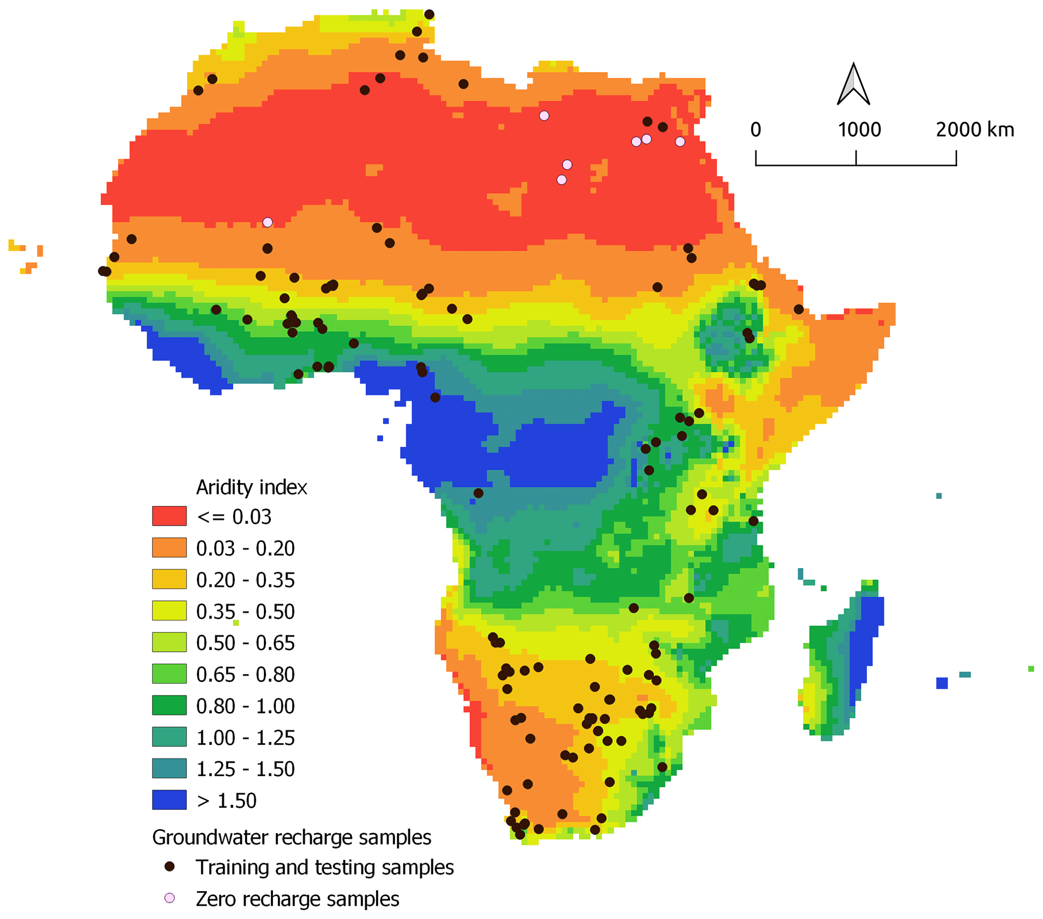
Figure 1 Data samples used for model training and testing, alongside zero-recharge points omitted in the initial variable importance analysis, compiled by MacDonald et al. (2021) in relation to the aridity of the region. Aridity index data were obtained from the CRU TS dataset (Harris et al., 2020).

2.3 The dataset of explanatory factors

Predictors related to climate, land use, soil type and hydrogeology, in particular those used by MacDonald et al. (2021), were considered to have the highest explanatory power in estimating groundwater recharge. According to the earlier study, precipitation dominates all other signals. Consequently, the same dataset on precipitation for the time period 1981–2010, originating from Climate Research Unit gridded Time Series (CRU TS) (Harris et al., 2020), was used to replicate its results. CRU TS is created by interpolating monthly climate anomalies obtained from numerous international weather stations, giving a global gridded dataset at a spatial resolution of 0.5°. Gridded data on remaining explanatory factors (MacDonald et al., 2021) were obtained from the same sources as in the original analysis. Potential evapotranspiration, aridity index and the number of wet days were provided alongside precipitation data by the CRU TS dataset. Normalised difference vegetation index (NDVI) data are provided by NASA's Moderate Resolution Imaging Spectroradiometer (MODIS) satellite product at a spatial resolution of 0.05°. Aquifer domain data were obtained from an earlier study by the British Geological Survey (MacDonald et al., 2012); soil group information derives from the Soil Atlas of Africa developed by a joint research effort of the European Union and FAO (Jones et al., 2013). Land cover data were extracted from the Historical Land-Cover Change and Land-Use Conversions Global Dataset based on HYDE 3.1 at a resolution of 0.5° (Meiyappan and Jain, 2012). Additionally, based on the latest literature findings, a range of other factors were identified as potentially insightful for this investigation (Mohan et al., 2018; Moeck et al., 2020). Of these, two variables (elevation and soil moisture) were incorporated into the models. The corresponding datasets were obtained from NASA's Shuttle Radar Topography Mission (SRTM) digital elevation version 4 and Famine Early Warning Systems Network Land Data Assimilation System (FLDAS) Noah Land Surface Model L4 products. Using meteorological variables from MERRA-2 analysis as forcing data, the FLDAS model, Noah 3.6.1, produced global estimates of land surface variables at a spatial resolution of 0.1°.

To create a groundwater recharge map at a spatial resolution of 0.1°, additional datasets of higher resolution from the Consultative Group on International Agricultural Research Consortium for Spatial Information (CGIAR-CSI) are employed for potential evapotranspiration and aridity. They are both modelled at a spatial resolution of 0.01°, using long-term monthly-averaged climate data from WorldClim. Also, another precipitation dataset of a higher resolution (Climate Hazards Group InfraRed Precipitation with Station data (CHIRPS) version 2 at a spatial resolution of 0.05°) is used for developing both RF and LMMs. CHIRPS data are produced by combining models of terrain-induced precipitation enhancement with interpolated ground-based station data and gridded satellite-based precipitation estimates from NASA and NOAA (Funk et al., 2015). A summary of the data sources for each variable, alongside the maps of spatial distributions of all explanatory factors, is given in Table S1 in the Supplement.

2.4 Random forest model

Random forest (RF) is an ensemble machine learning method for classification and regression based on randomised decision trees (Breiman, 2001). The fundamental concept behind the algorithm is that an average of the prediction probabilities of a large number of models outperforms any of the individual models in terms of accuracy. Consequently, RF, assembling an average model out of a large number of decision trees, is superior to just one model (one decision tree), which is very sensitive to outliers, unstable and tends to overfit. RF inherits most of the advantages of decision trees: the ability to handle both numerical and categorical input data, the lack of a need for data preparation such as input data normalisation, and robustness against multicollinearity of features. The theory and technical description of a decision tree algorithm and subsequently the random forest regression are introduced by Breiman et al. (1984) and Breiman (2001).

When training a RF model, every contributing decision tree is built based on a subset of training data drawn with replacement (bagging) so that the same sample can occur multiple times or might be omitted in a single tree creation process. About two-thirds of these samples are used for training, while the remaining “out-of-bag” (oob) samples are used for internal cross-validation, resulting in an oob performance score for the entire random forest model (Breiman, 2001). Additionally, the nodes in an individual tree are split using the best split predictive variable from a selected subset of features that changes randomly across different trees. The actual tree training data, being a subset of the original model training set used for creating a RF, vary in the number of employed predictors and in the number and composition of training samples across different decision trees. As a single tree tends to overfit its training dataset, an average over a high number of decision trees greatly reduces the prediction variance and delivers a model that is relatively robust to outliers which could distort the performance of other algorithms such as neural networks.

2.5 Linear mixed model

The statistical model tested against the random forest model is a linear mixed model (LMM), a well-established method that is suitable for handling spatially dependent data. MacDonald et al. (2021) used this approach to generate a continental LTA groundwater recharge map at a spatial resolution of 0.5°. Here, their procedure is replicated to obtain a map at a higher resolution of 0.1° and to allow for the result-based comparison of RF and LMMs at both resolutions; LMM is an extension of a simple linear model that allows for both fixed and random effect terms. While fixed effects comprise all predictors, which have a fixed relationship with the response variable across all observations, random effects account for the fact that fixed effects are expected to be spatially dependent, as observations in one area are likely to be more similar than those further apart. The map generation procedure closely follows the steps from MacDonald et al. (2021); that is, the LMM is used to compute the empirical best linear unbiased prediction (E-BLUP) of LTA recharge at unsampled sites on a prediction grid. As the locations of LTA recharge observations exhibit spatial dependence, E-BLUP combines the predicted value from the fixed effects and interpolated random effects to account for the variability among observation clusters and to minimise the expected prediction error variance. Further details on the developed model are described in Sect. S3 and MacDonald et al. (2021), whereas the theoretical description of the LMM can be found in Lark et al. (2006).

2.6 Residual kriging

Residual kriging is applied as a part of the procedure to compute E-BLUP of LTA recharge at a spatial resolution of 0.1° to minimise the expected squared prediction error. As the input data values for the LMM at 0.1° come from related predictor datasets as used for the LMM by MacDonald et al. (2021) and the residuals most likely exhibit similar patterns, the same assumptions are made regarding the choice of initial variogram parameters, covariance function and model fitting method. The final interpolation setup, including optimised model parameters, is described in Sect. S3. Residual kriging is also applied on top of the prediction results from the RF model. As algorithmic modelling (unlike parametric modelling) does not make any assumptions about the underlying process from which the observations originate, the spatial dependence of observations is not taken into consideration at any point by the base RF model. However, we explicitly account for variability in LTA recharge observations around the fitted values by investigating the residuals and performing kriging-type interpolation so that the correction of RF results is carried out under the assumption that the LTA recharge observations are likely to be similar for all unsampled sites in the proximity to the sampled sites.

2.7 Model development

The computer code developed in this analysis is written in Python 3.9 and R 4.2.0 and is available on GitHub at https://github.com/pazolka/rf-groundwater-recharge-africa (last access: 28 June 2024). The main code is partitioned into multiple Jupyter Notebooks, the names of which correspond to the names of the major steps of the analysis. The processed input raster files, derived from data freely accessible online, are available through an open-access repository linked to this paper.

The random forest implementation used in this study is RandomForestRegressor from Python library scikit-learn version 0.24.2. To generate a LMM based recharge map at 0.1°, the steps described by MacDonald et al. (2021) were followed using R library spaMM version 3.11.14. Residual interpolation applied in addition to RF and LMM results was performed using R library gstat because of more advanced variogram fitting options.

For interactive inspection of LTA recharge maps generated using developed models, the results were visualised using the Python package geemap (Wu et al., 2019; Wu, 2020).

2.7.1 Input data processing

All data were obtained in the form of GeoTIFF raster files (WGS84 projection), using both data provider websites and the Google Earth Engine platform. Time series for precipitation and soil moisture were averaged for the period 1981–2010 to obtain gridded long-term mean values commensurate with the temporal resolution of recharge observational data. Where necessary, input grids were rescaled to an appropriate resolution of 0.5 or 0.1°. Continuous point data were upscaled using bilinear interpolation, whereas the mode resampling method was applied to categorical data.

To ensure the consistency of the training data, the predictor values were sampled at each groundwater recharge observational point, resulting in two input datasets, one for each spatial resolution of interest.

2.7.2 Training and testing datasets for the random forest model

RF is a supervised ML algorithm. It uses labelled training data to construct a function inferring the desired output value from an input object in a process called model training. Apart from the training dataset, a testing dataset is typically employed to assess the ability of the algorithms to generalise from the training values to unseen data. As the RF model employs a form of internal cross-validation and builds each decision tree using only a subset of the training data, as outlined in Sect. 2.4, all recharge samples were used to build the final models used for predicting recharge values on the continental scale. In that step, model validation using a separate testing set was omitted and the out-of-bag score was used to check the generalisation ability of the final models. However, explicit partition of data into training and testing data consisting of 88 and 39 recharge samples (70 % and 30 %, respectively, following Nguyen et al., 2021) was performed for different subtasks in this study that required external validation, such as hyperparameter optimisation and performance assessment.

2.7.3 Performance metrics

The goodness of fit of models is primarily evaluated by calculating the coefficient of determination R² of the modelled and observed values, expressed as

$$\begin{array}{}\text{(1)}& R^{\mathrm{2}}=\mathrm{1}-{\displaystyle \frac{\sum _{i=\mathrm{1}}^n{\left(y_i-\widehat{y_i}\right)}^{\mathrm{2}}}{\sum _{i=\mathrm{1}}^n{\left(y_i-\stackrel{\mathrm{‾}}{y}\right)}^{\mathrm{2}}}},\end{array}$$

where y_i is the observed ith value, $\widehat{y_i}$ is the predicted ith value and $\stackrel{\mathrm{‾}}{y}$ is the mean value. Also, the out-of-bag (oob) performance score, a random-forest-specific metric of internal model validation, is investigated after each model training. R² is a measure of goodness of fit in capturing the variance and is expressed in relative values; therefore, root mean squared error (RMSE) is employed to quantify the absolute fit of the model. Apart from calculating the quantitative performance metrics, a visual analysis of a plot of observed versus modelled values and plots of observed and modelled values versus residuals were undertaken to inspect the presence of possible problems in the underlying data.

2.7.4 Data transformation

The LMM assumes the normality of residuals so that log transformation of LMM input data was required. The RF algorithm is non-parametric and makes no assumptions about the underlying statistical nature of the data. Predictive variables may be numerical or categorical, follow any distribution, and have different scales, requiring no extensive transformation. Although non-parametric models are rarely affected by skewness in the dependent variable, transforming the response variable can lead to predictive improvement in some cases (Boehmke and Greenwell, 2019). A preliminary check suggested that log transformation does not significantly improve the predictive ability of the random forest algorithm. However, to increase the prediction performance of low recharge values and to make the treatment of dependent variable consistent across the models, log transformation was applied to RF input data as well. The output data were back-transformed to the original scale. A similar transformation procedure was applied in other random forest applications (e.g. Wheeler et al., 2015; Ouedraogo et al., 2018).

2.7.5 Hyperparameter tuning

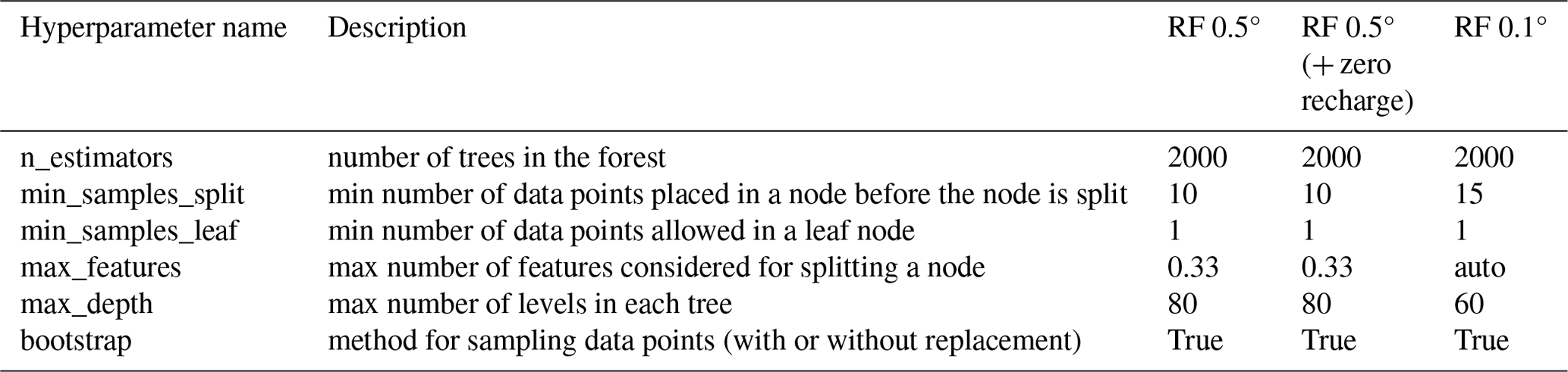
The RF model has two important user-defined hyperparameters: the number of decision trees and the number of randomly selected predictors used to split the nodes. Optimisation of these parameters can significantly reduce the generalisation error (Breiman, 1996; Peters et al., 2007). Concerning the number of trees, this value can be as large as possible since RF does not overfit and is computationally efficient and parallelisable (Breiman, 2001; Probst and Boulesteix, 2017); this study utilised 2000 decision trees. The recommended number of randomly selected predictors for each node split in a regression tree is the number of all predictors divided by three (Breiman, 2001; Hastie et al., 2009). Other minor hyperparameters were tuned using the random search technique with threefold cross-validation across 100 different combinations. Their values are summarised in Table 1. The hyperparameters were optimised again when adding zero-recharge samples to the recharge dataset and when using input data at a spatial resolution of 0.1° in further analysis.

Table 1 Optimal random forest hyperparameters found through random search with cross-validation for different random forest model variants used in this study.

2.7.6 Random forest models for LTA groundwater recharge in Africa

Complementary to the development of a RF model for continental LTA groundwater recharge, a simple predictor importance analysis using the RF's built-in feature importance was performed (see Sect. S5a). As the result, the predictor list for the final RF models used to generate maps was reduced to contain five variables (precipitation, soil moisture, NDVI, potential evapotranspiration and aridity index), as land cover, aquifer group, soil group and elevation were found to have a negligible effect on the explanatory power of the model.

The creation of a continental recharge map at a spatial resolution of 0.5° incorporated the selected variable set and the optimised hyperparameters. A single RF model was trained using all available samples. Finally, recharge values were predicted for the whole domain, and model performances in terms of R² and RMSE values of both the RF model and the LMM by MacDonald et al. (2021) were compared. Additionally, the absolute and relative spatial differences in recharge estimates between the models were obtained and investigated. A similar procedure was applied to obtain continental recharge values at a spatial resolution of 0.1° using higher-resolution predictor data, with an additional step needed to create a LMM at 0.1° by replicating the procedure by MacDonald et al. (2021).

Another pair of LTA recharge maps – at 0.5 and 0.1° – was created by extending the results of base RF models and interpolating the residuals from the RF predicted value and the observed LTA recharge. Section 3.2.2 and 3.3.3 compare the continental maps generated by base and kriged RF models and the LMM at the respective resolutions.

Although samples within aquifers where no modern recharge was detected were explicitly excluded from the variable sensitivity analysis and from the principal recharge modelling due to the assumed lack of causality between the predictors and the recharge, another recharge map was created to assess the influence of the inclusion of zero-recharge samples. As the previously found optimal hyperparameters might have become suboptimal after the inclusion of seven extreme values, hyperparameter tuning was performed again. A new RF model was trained using all 134 recharge samples and applied to the feature data of the whole domain to predict the recharge. Finally, the absolute and relative spatial differences between the recharge map obtained using the principal model and the model including zero-recharge samples were investigated. These results are presented in Sect. 3.2.1.

Additionally, a supporting sensitivity analysis was carried out to investigate the influence of different input precipitation datasets on the continental LTA recharge map at the spatial resolution of 0.5°. The results confirmed that the choice of the precipitation data source has a considerable impact on predicted values, as the precipitation signal is dominant over other predictors and the RF model directly reflects the spatial distribution of the precipitation data and accentuates differences between the individual datasets (see Sect. S5b). Further, the 90 % prediction intervals for the LTA recharge maps were constructed using quantile regression forest (QRF) (see Sect. S6). The average prediction of LTA recharge produced by RF is very highly correlated with the median prediction from QRF (R²=0.99). The accompanying maps visualise lower and upper bounds for the prediction interval at each grid cell (Figs. S12 and S13).

3 Results

To check the initial performance of the RF model before hyperparameter optimisation, a series of 100 models was built. The R² values of training and testing sets ranged between 0.94 and 0.96 and 0.28 and 0.80, respectively. The oob score oscillated between 0.57 and 0.73. It was possible to trade some accuracy on the training set for more accuracy on the testing set through tuning minor hyperparameters limiting trees capacity. Table 1 lists the optimal hyperparameters found through random search with cross-validation.

After applying the aforementioned hyperparameters to another series of 100 RF models, R² values of the training and testing sets ranged between 0.8 and 0.84 and 0.52 and 0.86, respectively. The oob score oscillated between 0.59 and 0.73. The optimised hyperparameters were used for generating recharge maps at spatial resolutions of 0.5 and 0.1°.

3.1 Evaluation of model performance on training and testing data

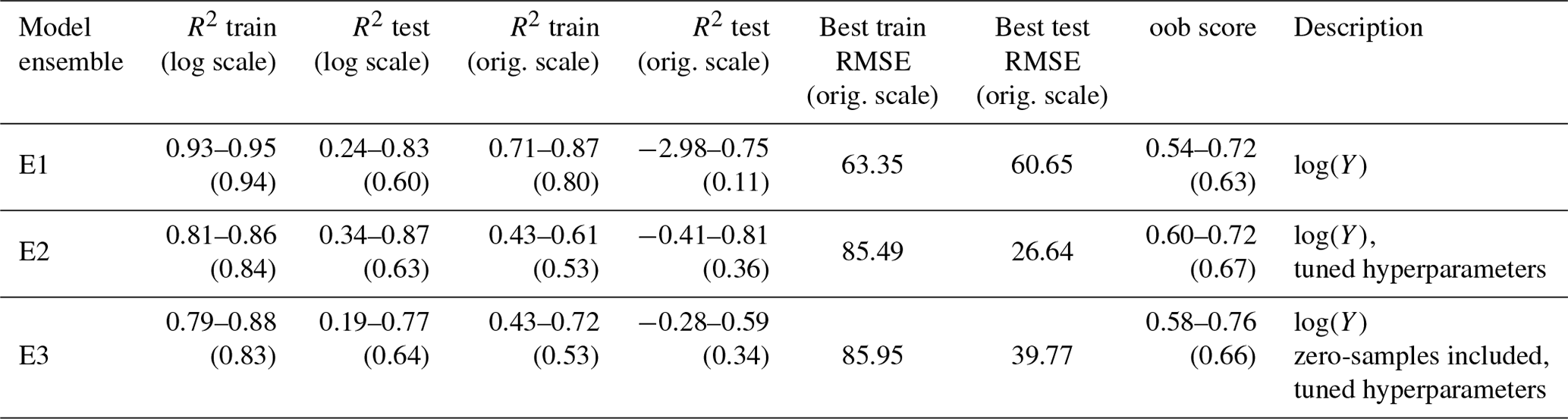
In addition to performance assessment based on the quantitative metrics (summarised in Table 2), a visual analysis of model residuals was performed based on a single model selected randomly out of the series of models (E2). The model R² values were 0.85 and 0.59 for the training and testing datasets, respectively, and the oob value was 0.69. The residual and predicted vs. observed plots across training and testing sets are included in Sect. S5c. High recharge values are mostly underestimated in both sets, as there are only a few measurements in the areas of high precipitation and high recharge. Also, some low recharge values are overestimated on a relative scale.

Table 2 Performance results of multiple random forest ensemble runs, each consisting of 100 random forest models, for both training and testing datasets. R² values, calculated for both log-transformed and back-transformed results, are expressed as an ensemble range, with the average value across all runs indicated within parentheses. RMSE values are calculated in the original scale for the best single model run in the series. Y refers to the target variable: groundwater recharge.

Several groundwater recharge sample points from the training and the testing set exhibit significant discrepancies between their observed and predicted values. Notably, this includes all samples obtained from Burkina Faso, situated in the semi-arid and tropical wet-and-dry climate zones. The model underestimates these samples (136 obs./38 pred., 221 obs./64 pred., 266 obs./126 pred.), which may indicate the influence and importance of preferential recharge pathways in this area (Mathieu and Bariac, 1996; Rusagara et al., 2022). A similar situation applies to two observational points in the semi-arid region in northern Ethiopia (185 obs./19 pred. and 167 obs./24 pred.), where recharge is highly variable on interannual scales (Yenehun et al., 2017). In general, the model underestimates extremely high recharge values in the humid equatorial regions of the Democratic Republic of the Congo (DRC), Cameroon and Benin. The recharge observations amount to 420, 941 and 491 mm yr⁻¹, whereas modelled values were 123, 125 and 167 mm yr⁻¹, which results in a few large residuals driving down the overall model performance. The substantial underestimation of recharge in the humid equatorial regions derives, in part, from a relative paucity of observations in these regions, compared to drylands. Interestingly, the predicted recharge for an observational point in Uganda, situated in the highlands, is overestimated (17 obs./67 pred.). In this area of runoff-dominated regime, recharge is restricted to years of exceptionally high rainfall (Taylor and Howard, 1999). Inadequate model performance here is possibly caused by the scarcity of data obtained from similar environments and the absence of topography-related variables in the set of explanatory factors.

3.2 Modelling groundwater recharge across Africa at 0.5° spatial resolution

Performance of the base RF model used for the groundwater recharge modelling on the continental scale is presented in Table 3. As the model was trained using all non-zero groundwater recharge sample points, its generalisation ability was assessed based exclusively on the oob score. Prediction performance on the training set, in terms of the R² value in the log scale, was compared with the performance of the LMM by MacDonald et al. (2021). Both models fit the observed recharge with similar results. The RF model was able to reproduce the results and, in some cases, provide marginally better predictions, e.g. for the recharge values $\mathrm{200}<Y<\mathrm{500}$, as illustrated in Fig. S9. The satisfactory out-of-bag value indicated that the model did not overfit the training data. However, both models did not generalise well for high recharge values.

MacDonald et al. (2021)

Table 3 Performance of random forest models used to predict groundwater recharge on the continental scale at a spatial resolution of 0.5°. Obtained R² values refer to the training set consisting of the entire available recharge sample data in the log scale, including or excluding the zero-recharge points. Metrics of the linear mixed models are included for comparison.

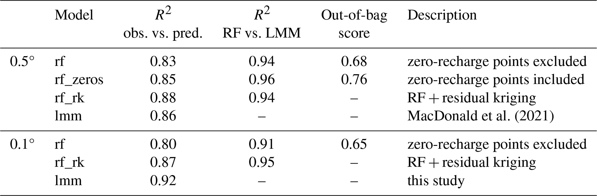
The combined model consisting of a RF model and residual kriging shows an improved fit in terms of R² value (0.88 vs. 0.83), but the effect is very localised, as the spatial dependence of residuals based on the fitted variogram is restricted to around 180–200 km.

3.2.1 Inclusion of zero-recharge samples

The inclusion of zero-recharge samples increased the overall fit of the RF model to observations (R²=0.83 vs. 0.89). However, this effect was caused predominantly by the inclusion of samples whose residuals were relatively small, driving the overall error down and thus increasing the score. Therefore, the RMSE values of non-zero recharge samples in both RF models were compared. A reduction from 79.5 to 76.5 mm yr⁻¹ suggests that the inclusion of zero-recharge samples did not negatively influence the recharge predictions of the remaining samples. The increased out-of-bag score confirmed that the model generalisation ability did not get compromised. The overall agreement of the LMM and RF model improved as well.

As illustrated in Figs. 2d and 3, the inclusion of zero-recharge samples mostly impacted recharge predictions in hyper-arid regions of northern Africa, although in absolute terms this was equivalent to a decrease from less than 2 mm yr⁻¹ to nearly zero recharge. It also contributed to modelled values being up to 10 % to 20 % higher in the tropics, in particular in the Congo Basin. The modelled values across other parts of Africa remained mostly unchanged. Curiously, there is a slight rise in the recharge values along the borderline between the southern Sahara and the Sahel.

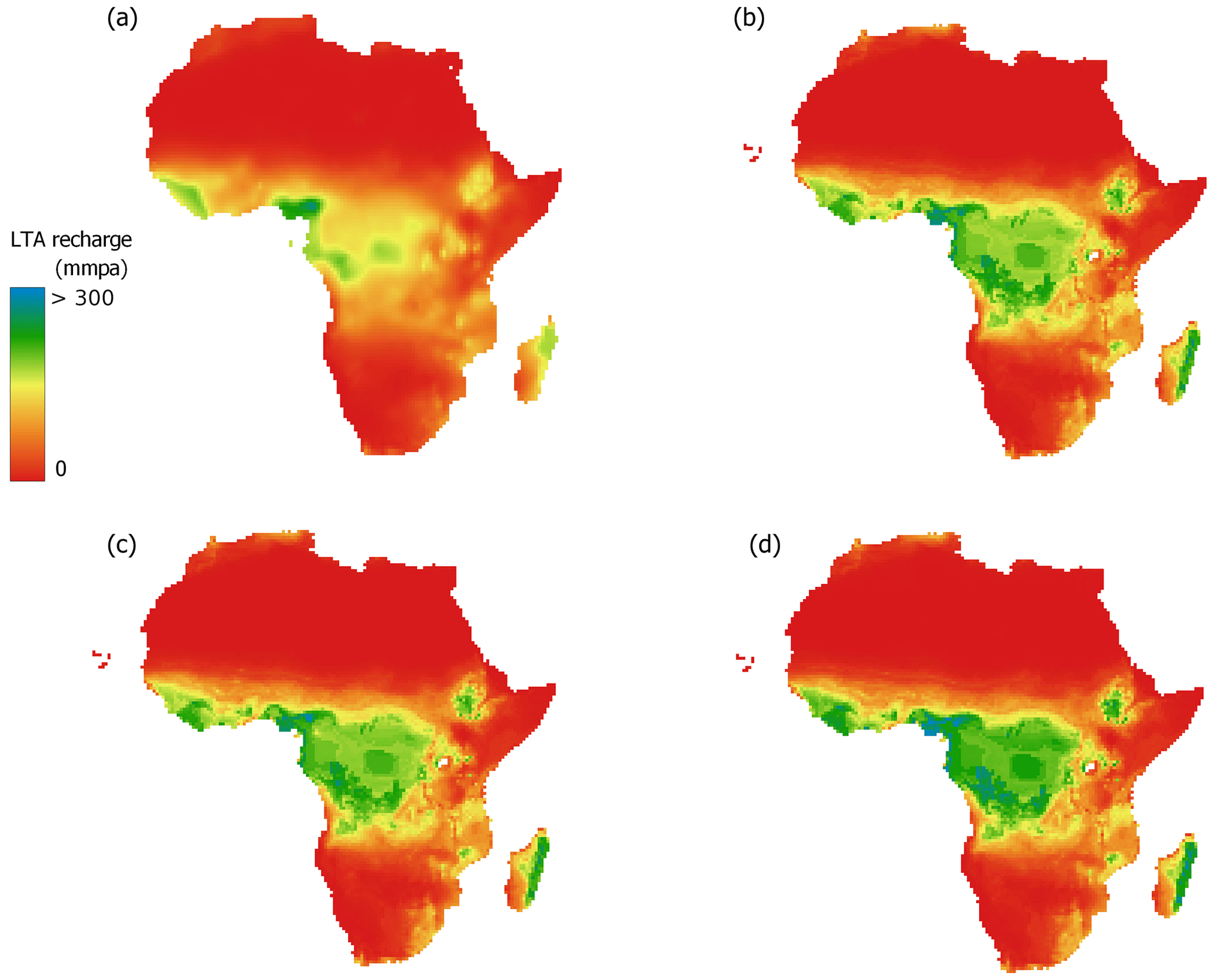
Figure 2 Comparison of LTA groundwater recharge maps for continental Africa at a spatial resolution of 0.5°, obtained using a linear mixed model by MacDonald et al. (2021) (a) and three variants of random forest model: base random forest model (b), random forest with additional residual kriging (c)and random forest applied to a dataset extended by sample points from zero-recharge sampling sites (black dots) (d). Differences between these models are detailed in Sect. 3.2.2.

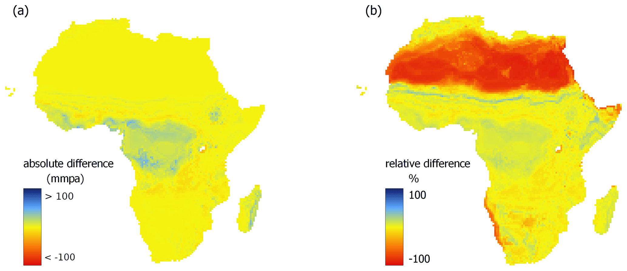
Figure 3 Effects of including zero-recharge observations on continental LTA recharge maps generated using random forest. Absolute (a) and relative (b) spatial differences between groundwater recharge maps for continental Africa, obtained using two variants of random forest model (without and with zero-recharge observations – Fig. 2b, and d) at the spatial resolution of 0.5°. The difference was calculated as follows: RF (zero-recharge sites included) – RF (base).

3.2.2 Spatial differences between models at 0.5° spatial resolution

The recharge maps generated by the RF models demonstrate a higher level of spatial detail on regional scales than the LMM-derived recharge map (Fig. 2). Recharge values predicted by RF models vary more significantly in one region (e.g. in the tropics), whereas the LMM predictions are smoothed out by kriging interpolation. Such a high level of spatial variability in recharge can be expected in the tropics due to the inclusion of a greater number of high-resolution explanatory factors: precipitation, soil moisture, aridity index, potential evapotranspiration and NDVI, as the variability in recharge is associated with the variability in the predictors, especially since there are no observations from this region that could constrain it.

The highest absolute differences in recharge estimates (Fig. 5) occur south from the Equator, in the tropical and humid wet-and-dry climate zones. The RF model predictions are more than 75 mm yr⁻¹ higher than the LMM values. Other areas exhibiting similarly high differences are the Ethiopian Highlands and the western part of Madagascar. The high relative difference in modelled values in the Sahara is simply due to the difference between very low recharge values predicted by the RF model (<1.5 mm yr⁻¹) and negligible LMM-derived recharge (<0.1 mm yr⁻¹). The underestimation of recharge values by the RF models in comparison to the LMM along the borderline between the southern Sahara and the Sahel is caused by the fact that the RF recharge values increase more gradually when moving towards the Equator. The most substantial difference in both absolute and relative recharge is found in Angola and in the southern part of the DRC, in the tropical savannah climate. Here, RF model-derived values are twice as large as the LMM predictions (160–240 mm yr⁻¹ vs. 80–120 mm yr⁻¹). However, no observations are available from this region to assess the accuracy of these estimates.

The effects of residual kriging added to the base RF model are very localised (Fig. 5c and g), leading to a correction of RF-predicted values and pixels within a small radius around the fitted values (180–200 km). This indicates that the base RF model at 0.5° can capture most of the spatial variation in the observational data. The difference in predicted LTA recharge ranges between ±17 % and 39 %, depending on the sample point (e.g. Burkina Faso: from 29 to 44 mm yr⁻¹, +39 %; Libya: from 1.3 to 0.8 mm yr⁻¹, −38 %; Cameroon: from 265 to 334 mm yr⁻¹, +26 %).

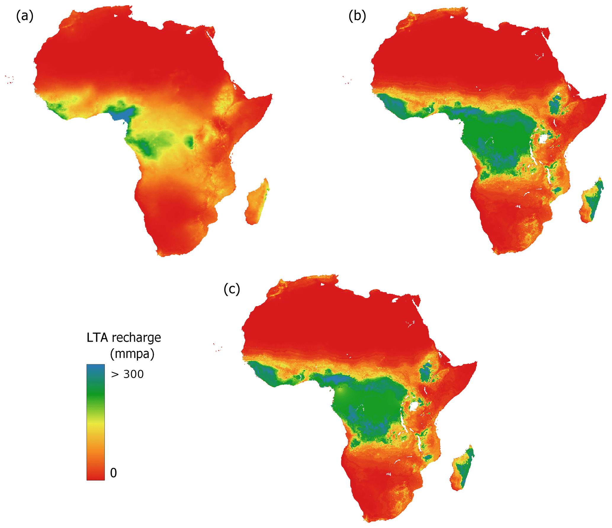
Figure 4 LTA groundwater recharge modelled at a spatial resolution of 0.1° using (a) linear mixed model with residual kriging, (b) base random forest and (c) random forest with residual kriging.

3.3 Modelling groundwater recharge across Africa at 0.1° spatial resolution

3.3.1 Random forest-based LTA groundwater recharge maps and comparison with 0.5° model

Recharge maps at the spatial resolution of 0.1° obtained employing a RF model with and without residual kriging, built using the explanatory factors (Table S1) and the corresponding optimal hyperparameters (Table 1), are illustrated in Fig. 4. Apart from a higher resolution, these models differ from the models at the spatial resolution of 0.5° primarily by employing predictor datasets from other sources and by using recalculated hyperparameters. At 0.1°, the influence of additional residual kriging is also very localised. The fitted residual variogram demonstrates only a slightly higher spatial dependence of residuals up to around 200–250 km. The predictive performance of both versions of a RF model, in terms of the R² value in the log scale, is comparable to the performance of the models at 0.5° (Table 3). The RF model with residual kriging explains 7 % more variance than the base RF model.

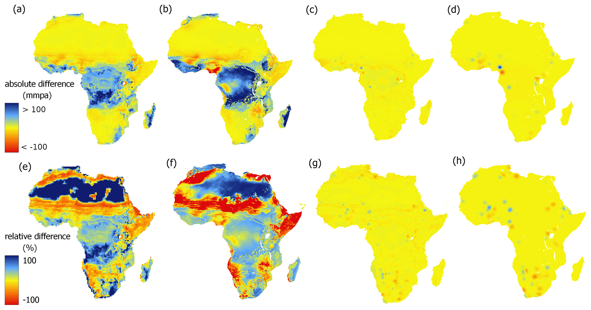
Figure 5 Absolute (a–d) and relative (e–h) spatial differences between groundwater recharge maps for continental Africa: (a, e) random forest model with residual kriging and linear mixed model at 0.5° RF_RK – LMM, (b, f) random forest model with residual kriging and linear mixed model at 0.1° RF_RK – LMM, (c, g) random forest model with residual kriging and base random forest model at 0.5° RF_RK – RF, (d, h) random forest model with residual kriging and base random forest model at 0.1° RF_RK – RF.

Moving from 0.5 to 0.1°, several substantial differences in regional groundwater recharge are evident using both RF models. In the most humid areas of western Africa and the Gulf of Guinea, the modelled recharge reached 250–350 mm yr⁻¹. Also, a significant increase in the recharge in the eastern part of the DRC was modelled (from 160–180 to 220–260 mm yr⁻¹). Notably, high recharge values were predicted in Morocco, reaching up to 120–170 mm yr⁻¹, compared to 10–30 mm yr⁻¹ modelled by the lower resolution RF models. A possible anomaly in the soil moisture dataset around the South African cities of Pretoria and Johannesburg (0.4 m³ m⁻³ vs. 0.24 m³ m⁻³ in the neighbouring cells) led to a high local recharge estimate. However, high soil moisture content in the highly urbanised areas might be linked to extensive irrigation and therefore cause elevated recharge rates.

3.3.2 Linear mixed model-based LTA groundwater recharge map and comparison with 0.5° model

The LMM at 0.1° scores a marginally better R² than the original LMM at 0.5° by MacDonald et al. (2021) (0.92 vs. 0.86; Table 3). The spatial patterns are unchanged which is expected, as both LMMs rely on precipitation datasets of similar spatial distributions (CRU TS at 0.5° and CHIRPS at 0.1°) – see the additional precipitation sensitivity analysis in Sect. S5b. With a higher resolution precipitation dataset, more small-scale details become visible (Figs. 2a and 4a). For example, LTA recharge values in Morocco are twice as high at higher resolution: 20–30 mm yr⁻¹ vs. 60–70 mm yr⁻¹; in the eastern DRC: 120 mm yr⁻¹ vs. 240 mm yr⁻¹; in the Republic of the Congo: 190 mm yr⁻¹ vs. 250 mm yr⁻¹. A decrease in predicted LTA recharge is found in some places like Mozambique and Madagascar, where no observations are available. Also, at the higher resolution, exceptionally high observed recharge values lead to the creation of distinct spikes in localised, considerably higher modelled recharge, e.g. the observations in Cameroon (obs. 941, pred. 469 mm yr⁻¹) and the DRC (obs. 420, pred. 250 mm yr⁻¹).

3.3.3 Spatial differences between models at 0.1° spatial resolution

At 0.1°, spatial differences between all models are visibly more prominent than at the lower resolution, as shown in Fig. 5. The addition of residual kriging to the base RF model leads to higher variation in predicted recharge values in the entire domain (Fig. 5h). The biggest absolute changes are present in the humid areas of central Africa, almost symmetrically around the Equator. These increases in results of the extended RF model may be driven by high residual values from two observations: in Cameroon and the DRC/Republic of the Congo. Other significant increases occur in Ethiopia and western Africa. Decreases are driven by negative residuals primarily in Morocco, Côte d'Ivoire and along the west edge of the East African Rift.

Similarly to the results at 0.5°, RF models predict higher recharge rates in northern Africa than the LMM. The extraordinarily high recharge observation in Cameroon drives a high local anomaly in DRC due to a high residual in the LMM, which is more localised in the LMM than in RF models. The LMM-derived map resembles closely the input precipitation map, as precipitation is the only explanatory factor, whereas RF models also incorporate signals from the remaining employed predictors: soil moisture, NDVI, aridity index and potential evapotranspiration. There is therefore a significant difference in recharge predictions in central Africa, where there are no observations to constrain the models.

4 Discussion

4.1 Random forest (RF) vs. linear mixed model (LMM)

The results of this study confirm that the RF technique is able to model the LTA groundwater recharge with an accuracy comparable with the linear mixed model by MacDonald et al. (2021). The overall fit of both LMM and RF models to observations was comparable, as indicated by high R² values. It confirmed that a LMM based only on precipitation was able to perform on the observational set as well as a more sophisticated RF model driven by five variables. When modelling groundwater recharge on a continental scale, the RF model resulted in a considerably higher spatial variability of the recharge, especially in the tropics. This was expected given that very high spatial variability is also modelled in other parts of the world (Shamsudduha et al., 2015) and that there is a significant precipitation variability in the tropics, as confirmed by the variability in the rainfall-correlated datasets (precipitation, soil moisture, NDVI). The ability of the RF model to capture a small-scale variability in the input datasets and to mirror it in the recharge predictions, given sparse observations, is a clear advantage over the LMM. The latter produced a recharge map with values that are smoothed out through kriging interpolation, consequently losing the degree of detail of the high-resolution predictor datasets.

Apart from the improved spatial level of detail, the RF model was able to detect additional areas of recharge such as coastal regions of Morocco and Algeria. Other substantial spatial differences occurred in all climatic zones, especially south of the Equator and in south-east Africa. This was possibly caused by the extended predictor set and by different model structure.

4.2 Effects of adding residual kriging

Additional residual kriging on top of RF-based recharge estimates does not have a significant effect on the prediction at both spatial resolutions. Compared with the residual variograms of the LMMs, RF-based residual variograms exhibit considerably smaller semi-variance, which indicates that the base RF model captures the variance in LTA groundwater recharge predictions well, based only on the predictor dataset. There is no strong smoothing effect as seen in the LMM.

4.3 What insight do we gain from higher resolution?

The observed differences in the low- and high-resolution LTA groundwater recharge maps have two likely origins. Firstly, as both LMMs and RF models heavily depend on the employed precipitation datasets, some of the spatial differences might naturally be caused by using rainfall data from different sources. Some global precipitation datasets exhibit significant discrepancies in the long-term mean over equatorial western Africa because of their low gauge densities, as well as in interannual and decadal variations in rainfall over the Congo Basin (Sun et al., 2018). In this analysis, regional rainfall discrepancies could have induced small-scale differences that became apparent in both LMMs and RF models, when comparing their results at different resolutions. Both data-driven models require careful input selection and quantification of uncertainties in the input dataset, as the quality of output can only be as good as the quality of the input dataset. Secondly, differences could also result from small-scale variability in predictor datasets at a very high resolution. Due to the ability to retain a high spatial variability in predictor datasets (despite sparse observations), the RF model could be used for an extended study that incorporates observations of focused recharge. Such an approach, combined with high-resolution data on the occurrence of surface water and more advanced soil- and aquifer-related predictors, could identify areas of small-scale, focused recharge that largely contributes to aquifer replenishment in drylands (Cuthbert et al., 2019; Seddon et al., 2021).

4.4 Bias towards dry regions

It is apparent from the LTA recharge map generated using regression combined with residual kriging that the sample of observations is not sufficient to create a model that generalises well for observations in the humid regions. High residuals are present for the great majority of sample points in the tropical wet regions of high aridity index (e.g. observations in Uganda, Burundi, DRC, Cameroon and south-west Nigeria), where the difference amounts to 25 %–60 %. These residuals lead to localised spikes in the predicted recharge around the fitted values, mostly visible in the LMM-derived maps. Due to the very limited number of observations in the equatorial humid regions, the models are not well constrained at high mean precipitation rates, which is also reflected in the high uncertainty in these areas (see the 90 % prediction intervals, Sect. S6). The LTA groundwater recharge predictions are very likely largely underestimated. Additionally, the high number of observations from drylands dominates the training of the RF model and fitting of the LMM, leading to the conclusion that climatic and meteorological factors can explain a large majority of variance. Other topographic and geological factors, alongside a higher number of observations in equatorial humid areas, need to be incorporated into the models to better predict higher recharge rates.

4.5 Uncertainty and sensitivity of the random forest model

Regional recharge estimates should be interpreted with caution, as they depend on input data quality and the spatial distribution of observations. Despite using high-quality, auxiliary input datasets, these data introduce uncertainty into this analysis, as has the data processing through standard techniques such as bilinear interpolation. In the following, uncertainty related to the choice of the modelling algorithm is discussed.

Both RF and LMM models were sensitive to the changes in input datasets, especially in the areas of limited observations. In addition, the inclusion of the Saharan zero-recharge points had a substantial impact on the groundwater recharge predictions by the RF model in other areas that lack observational data such as the following: in central Africa, the Horn of Africa and Namibia. The effects of additional residual kriging are visible across the whole domain, including the areas where no observations could constrain corrected predictions.

Additional potential stability issues were observed during the supplementary variable selection process. As the RF model is characterised by a data-dependent tree structure, the composition of the training and testing datasets had a large impact on the model performance. In some extreme cases, the model was unable to generalise from the training samples to the unseen (testing) data, as indicated by a disparity of the R² values in a series of RF models calculated in that process (see Table 2). All these results highlight a possible problem with the suitability of the model in this domain with the current training dataset of groundwater recharge observations. The observational data are highly skewed to a few high recharge samples, which led to high model residuals at these points. This is a fundamental problem of the loss of prediction accuracy with the increasing observed values, and the incorporation of additional high-recharge data could possibly improve the model performance and constrain high differences in the predicted recharge in the observation-sparse equatorial regions and reduce the current bias towards drylands. Nevertheless, the RF technique was able to reproduce the results of the LMM by MacDonald et al. (2021), which indicates that further prediction improvement depends heavily on the quality of input data and the inclusion of more observational points.

Contrary to other ML algorithms, the RF model does not require extensive hyperparameter optimisation, so only a small performance gain can be achieved through model tuning (Probst et al., 2019a). Although this was indeed the behaviour observed when comparing the performance metrics before and after the hyperparameter search in this study (Table 2), hyperparameter tuning led to a substantial reduction in predicted recharge in some regions where no observations were present, as evident from Fig. 2b (with model tuning) and Fig. S7a (without model tuning). In some cases, the difference reached up to 150 mm yr⁻¹.

A similar situation was detected when comparing the influence of various precipitation datasets. Although the spatial differences between the CRU and CHIRPS precipitation datasets were relatively small and the other predictor datasets remained mostly unchanged apart from their resolution, the recharge values obtained at the spatial resolutions of 0.1° (Fig. 4b) and 0.5° (Fig. 2b) differed significantly not only in the humid areas along the Equator but also in the semi-arid regions of north-west Africa. A sensitivity analysis to model hyperparameters would be a natural extension to this study and investigate the extent of uncertainty in the modelled recharge linked to hyperparameter tuning. Also, a more sophisticated hyperparameter search technique could be employed in the future (Probst et al., 2019b). However, the inclusion of more groundwater recharge measurements would likely constrain the variance in the modelled values caused by hyperparameter tuning.

The RF technique makes no assumptions about the distribution of the underlying data and thus is non-parametric. Although it can deal with a limited sample size (Scornet et al., 2015), some research applications need very large datasets to achieve accurate predictions (e.g. for medical prediction problems, van der Ploeg et al., 2014). In the context of continental-scale long-term groundwater modelling with sparse and unevenly distributed observations, the observed variance in the modelled recharge values across the continent suggests that the current dataset size and sample distribution leads to high uncertainty. The accompanying work presented in Sect. S6 shows that prediction intervals in humid equatorial regions with limited observations are very wide. This suggests that a more diverse and larger training dataset that is better able to represent the climatic and geological diversity and the size of the study area might achieve significantly better results.

4.6 Future work

The new RF model could be extended by other explanatory factors and more measurements in high recharge areas in order to improve model fits as the existing distribution of values is not well explained by the variability in the currently employed climatic and vegetation predictor variables. Moeck et al. (2020) point out that recharge estimates based solely on climatic variables can be misleading and that vegetation and soil structure have an explanatory power too. It is a reasonable assumption and this could be addressed in a future study that looks more carefully into variable importance and focuses on interpretability of machine learning models. In this study, variables were selected for the model to match the data used previously in the linear mixed model by MacDonald et al. (2021); most of the input data are the same datasets. The observational dataset on groundwater recharge underwent a more thorough and transparent QA to give a curated dataset using techniques appropriate to the African environment. Interestingly, although local factors in soil and geology are important in controlling local recharge as shown by the residuals in the model, they do not improve the large-scale continental model (MacDonald et al., 2021). In the follow-up paper from Moeck et al. (2020), only climatic factors are used for global modelling (Berghuijs et al., 2022).

The modelling outputs of this study at both spatial resolutions can be compared directly with the output from large-scale process-based models such as WaterGAP (Müller Schmied et al., 2021) and PCR-GLOBWB (Sutanudjaja et al., 2018). When employing a RF model to an observational dataset from a different time window, other variables (e.g. total terrestrial water storage) can be employed to test the model, such as GRACE satellite data (e.g. Bonsor et al., 2018; Scanlon et al., 2022), which have been employed to identify inaccuracies in global hydrological model-derived decadal trends in terrestrial water storage (Scanlon et al., 2018).

More importantly, a modified approach to input data preparation could significantly improve model accuracy. West et al. (2022), based on the work by Winter (2001), proposed large-scale regionalisation and incorporation of the concept of recharge landscape units (RLUs) to group similar areas (in terms of climatic, land-cover/land-use, topographic and geological features, as well as occurrence of perennial and ephemeral waterbodies). Such an approach could capture important groundwater recharge factors that dominate locally, within a specific hydrogeological setting. As the observational dataset used in this study is biased towards arid and semi-arid regions, the use of the entire dataset for the continental recharge modelling without explicitly taking into consideration distinct regional differences and intracontinental diversity (tropical and humid vs. dry, upland vs. lowland) might effectively ignore significant local drivers. Although West et al. (2022) concludes that grouping based on the applied global datasets of selected predictors is insufficient for explaining the variability within individual RLUs, the combination of the concept of RLUs, comparative hydrology and machine learning could improve large-scale LTA groundwater recharge estimations; use of samples from other regions classified as similar RLUs would increase the number of observational points to train the algorithm and could potentially reduce the current bias towards drylands.

5 Conclusions

In this study, a random forest (RF) model was developed for the first time to predict long-term average groundwater recharge on a continental scale. It is capable of reproducing the results of a linear mixed model (LMM) developed by MacDonald et al. (2021) in terms of the model fit to the groundwater recharge dataset compiled in the aforementioned study. At a spatial resolution of 0.5°, the key advantage of the RF model over LMM is its greater ability to capture high spatial variability in the input dataset and to mirror it in the predicted recharge values. In this way, it has been possible to identify the areas of recharge that were previously unrepresented (e.g. in north-west Africa) and to map the variability in recharge at small scales, which is expected to be particularly characteristic of humid regions.

The use of the input dataset at a finer spatial resolution of 0.1° enabled the generation of a high-resolution continental recharge map that could inform country-level groundwater management decisions and support testing and calibration of mechanistic global hydrological models. However, the results should be interpreted with caution, primarily in regions of sparse observational data, due to high model uncertainty. This limitation was identified through the use of precipitation data from different sources, tuning of hyperparameters and the inclusion of zero-recharge sample points that were initially excluded from the analysis due to the assumed lack of causality between the precipitation and the groundwater recharge. The addition of residual kriging to the base RF model slightly improved its fit to high recharge observations, though the applied predictors (precipitation, potential evapotranspiration, aridity index, NDVI and soil moisture) were unable to explain those high recharge values. High residual values for the data points located in the Gulf of Guinea and in the DRC suggest that the model is not able to create a link between the current set of predictors and the few very high recharge observations. The incorporation of yet unidentified factors representing subsurface heterogeneity may improve the prediction accuracy of the model for these points and effectively allow us to incorporate focused recharge that is crucial to accurately assess the renewability of groundwater resources in the semi-arid regions, but it would require a significant amount of data engineering. Future work should also aim to incorporate the concept of “recharge landscape units”, which could help to capture the variability in dominance of individual explanatory factors across different hydrogeological environments. In general, the inclusion of more LTA groundwater recharge sample points, especially from tropical humid regions, could improve model predictions and reduce the current bias towards drylands in the input dataset. As the interest in groundwater resources in Africa is growing due to their resilience to short-term climatic variability, more groundwater recharge surveys are expected to be conducted across the continent, which will allow for the full use of RF's predictive potential.