To bucket or not to bucket? Analyzing the performance and interpretability of hybrid hydrological models with dynamic parameterization

Hydrological hybrid models have been proposed as an option to combine the enhanced performance of deep learning methods with the interpretability of process-based models. Among the various hybrid methods available, the dynamic parameterization of conceptual models using long short-term memory (LSTM) networks has shown high potential. We explored this method further to evaluate specifically if the flexibility given by the dynamic parameterization overwrites the physical interpretability of the process-based part. We conducted our study using a subset of the CAMELS-GB dataset. First, we show that the hybrid model can reach state-of-the-art performance, comparable with LSTM, and surpassing the performance of conceptual models in the same area. We then modified the conceptual model structure to assess if the dynamic parameterization can compensate for structural deficiencies of the model. Our results demonstrated that the deep learning method can effectively compensate for these deficiencies. A model selection technique based purely on the performance to predict streamflow, for this type of hybrid model, is hence not advisable. In a second experiment, we demonstrated that if a well-tested model architecture is combined with an LSTM, the deep learning model can learn to operate the process-based model in a consistent manner, and untrained variables can be recovered. In conclusion, for our case study, we show that hybrid models cannot surpass the performance of data-driven methods, and the remaining advantage of such models is the access to untrained variables.

1 Introduction

Rainfall–runoff models are useful tools to support decision-making processes related to water resources management and flood protection. Over the past decades, hydrological conceptual models have emerged as important tools for these purposes, finding widespread usage in academia, industry, and national weather services (Boughton and Droop, 2003). These models, known for their simplicity, computational efficiency, and ability to generalize, encode our understanding of hydrological processes within a fixed model structure. By connecting the various macroscopic storages (also known as buckets) through a network of fluxes, conceptual models try to emulate the internal processes occurring within a catchment. The accurate representation of these processes relies on calibrated parameters, which are adjusted to achieve consistency with observed data. Examples of widely used conceptual models include Hydrologiska Byråns Vattenavdelning (HBV) (Bergström, 1992), Sacramento (Burnash et al., 1973), GR4J (Perrin et al., 2003), Precipitation-Runoff Modeling System (PRMS) (Leavesley et al., 1983), and TOPMODEL (Beven and Kirkby, 1979), to name a few. Additionally, there are software tools available, such as Raven (Craig et al., 2020) and Superflex (Dal Molin et al., 2021), which facilitate the creation of customized models tailored to specific basin characteristics and key hydrological processes.

Despite the widespread use of conceptual models, data-driven techniques, particularly long short-term memory (LSTM) (Hochreiter and Schmidhuber, 1997) networks, have recently shown the potential to outperform conceptual models, particularly in large sample model comparison studies (Kratzert et al., 2019b; Lees et al., 2021; Feng et al., 2020). The improvement in performance can be attributed, partly, to the inherent flexibility of LSTM networks (LSTMs hereafter), which surpasses the constraints imposed by fixed model structures by effectively mapping connections and patterns through optimization techniques. However, the characteristic that allows LSTMs to excel in performance has also sparked criticism regarding their interpretability (Reichstein et al., 2019), owing to the fact that weights and biases in LSTMs lack clear semantic meaning, making it challenging to discern the underlying reasons for their decision and predictions. In recent years, notable advancements in linking hydrological concepts to the internal states of LSTMs have been made (Kratzert et al., 2019a; Lees et al., 2022), and we seek to further contribute in this research direction.

Reichstein et al. (2019) and Shen et al. (2023) indicate that combining process-based environmental models with machine learning (ML) approaches, into so-called hybrid models, can harness the strengths of both methodologies, leveraging the improved performance of data-driven techniques while retaining the interpretability and consistency offered by physical models. Among the various approaches proposed by the authors, one method involves the parameterization of physical models using data-driven techniques. Kraft et al. (2022) applied this method, with the idea that replacing poorly understood or challenging-to-parameterize processes with ML models can effectively reduce model biases and enhance local adaptivity. Moreover, their study demonstrated that the hybrid approach achieved comparable performance to process-based models. Feng et al. (2022) followed a similar procedure, in which the parameters of an HBV model were dynamically estimated using an LSTM network. Their study convincingly demonstrates the effectiveness of this approach, revealing its ability to achieve state-of-the-art performance that directly rivals purely data-driven methods when applied to the Catchment Attributes and Meteorology for Large-sample Studies (CAMELS) dataset (Addor et al., 2017) in the United States (CAMELS-US). In their study, Feng et al. (2022) implemented both static and dynamic parameterization techniques and observed that the latter led to slightly improved performance.

The dynamic parameterization of a process-based model is not a new idea. Lan et al. (2020) indicate that, historically, the most common approach to accomplish this is the calibration for different sub-periods. They support this statement by referencing over 20 studies on this subject published in the last 15 years. According to those authors, this method divides the data into sub-periods, considering seasonal characteristics or clustering approaches and proposing a set of parameters for each sub-period. The idea is to capture the temporal variations of the catchment characteristics.

Using an LSTM to give a dynamic parameterization of a process-based model may be seen as a generalization of this process. Specifically, one uses a recurrent neural network that analyzes a given sequence length, so the proposed parameters are context informed and reflect the current state of the system. The main difference is that the data-driven parameterization is much more flexible, as a custom parameterization can be proposed for each prediction, and it is not constrained to a typical small set of predefined sub-periods. Also, one can include as input to the LSTM any information that is considered useful to make an informed parameter inference, even if this is not used later in the conceptual part of the model.

However, it is important to note that Feng et al. (2022) warn about the flexibility of LSTM networks when used for dynamic parameterizations. They posed the hypothesis that, while applying dynamic parameterization increases the likelihood of achieving high performance, there is a risk of compromising the physical significance of the model, potentially resulting in the system behaving more like an LSTM variant rather than a hydrologically meaningful model. In other words, model deficits and ill-defined process descriptions might be compensated by the LSTM. Moreover, Frame et al. (2022) argue that adding any type of constraint, physically based or otherwise, to a data-driven model is only beneficial when such constraints contribute to the optimization process.

Motivated by the outcomes achieved in the aforementioned articles, our study aims to dig deeper into the coupling of LSTM and conceptual models. We believe that dynamic parameters provided by an LSTM allow the conceptual model to not only adapt to changes in the hydrological regime, which is physically reasonable (Loritz et al., 2018), but also to compensate for inherent deficiencies or oversimplifications within the model structure. More specifically, and guided by the warning given by Feng et al. (2022) and Frame et al. (2022), our study aims to address the following research questions:

1. Do conceptual models serve as an effective regularization mechanism for the dynamic parameterization of LSTMs?

2. Does the data-driven dynamic parameterization compromise the physical interpretability of the conceptual model?

To address the research questions at hand, we have structured our article as follows. In Sect. 2 we describe the structure and training process of the conceptual, data-driven, and hybrid models employed in this study. Additionally, we outline the details of the dataset used to train and test the rainfall–runoff models. In Sect. 3, after proving that the hybrid model performance is comparable with the LSTM, we conduct experiments to answer our first research question. By systematically modifying the conceptual model, we assess how different forms of regularization affect the overall performance of the hybrid model. This will allow us to better understand the effect of different conceptual models as regularization and the interaction between the data-driven and conceptual components. Furthermore, to address the second research question, we analyze the internal states of the conceptual model to evaluate how much physical interpretability the different variants of our conceptual model are keeping. Finally, we summarize our key findings in Sect. 4.

2 Data and methods

To answer the research questions stated in the previous section, we compared three types of models: purely data-driven (LSTM), stand-alone process-based models, and the hybrid approach. The first two types served as baselines in the different experiments we performed for the latter.

The first subsections of this section present an overview of the dataset utilized for training and testing our models. The second subsection describes the dataset used to evaluate the internal states of our process-based models. The last three segments explain the structures of the different models.

2.1 Dataset

To train and test our rainfall–runoff models, we used the CAMELS-GB dataset (Coxon et al., 2020a). This dataset contains information about river discharge, catchment attributes, and meteorological time series for 671 catchments in Great Britain.

To facilitate the comparison of our results with the studies of Lees et al. (2021, 2022), we maintained the periods for training (1 October 1980–31 December 1997), validation (1 October 1975–30 September 1980), and testing (1 January 1998–31 December 2008) from their studies.

2.2 ERA5-LAND

As outlined in the Introduction, one of the primary objectives of this study is to assess the physical consistency of our hybrid model. To achieve this, we conducted several tests, one of which involved comparing the unsaturated zone reservoir of the conceptual model with soil moisture estimates (details in Sect. 3.5). Following the procedure proposed by Lees et al. (2022)), we compared our model's results with data from ERA5-LAND (Muñoz Sabater et al., 2021). This dataset, based on a 9 km × 9 km gridded format, is a land component reanalysis of the ERA5 dataset (Hersbach et al., 2020). According to Lees et al. (2022), reanalysis data offer several advantages, including longer time series availability, easy transferability to basin-average quantities (consistent with the CAMELS-GB process) due to the gridded format, and global coverage, enabling its application in various locations. As our study region and testing period aligns with that of Lees et al. (2022), we utilized the NetCDF file provided by the authors, which was publicly accessible. We then extracted the values and normalized the data to a [0–1] range for comparative purposes. This normalization approach is consistent with Ehret et al. (2020), where they followed a similar process to assess the realism of the unsaturated zone soil moisture dynamics of a conceptual hydrological model.

ERA5-Land contains information about soil water volume at four different levels. Level 1 (swvl1) provides information at a depth of 0 to 7 cm, level 2 (swvl2) from 7 to 28 cm, level 3 (swvl3) from 28 to 100 cm, and level 4 (swvl4) from 100 to 289 cm. When using this information to evaluate our models, we consistently found higher correlations for all cases when compared against swvl3. Therefore, the results reported in Sect. 3.5 are associated with that depth.

2.3 Conceptual hydrological model

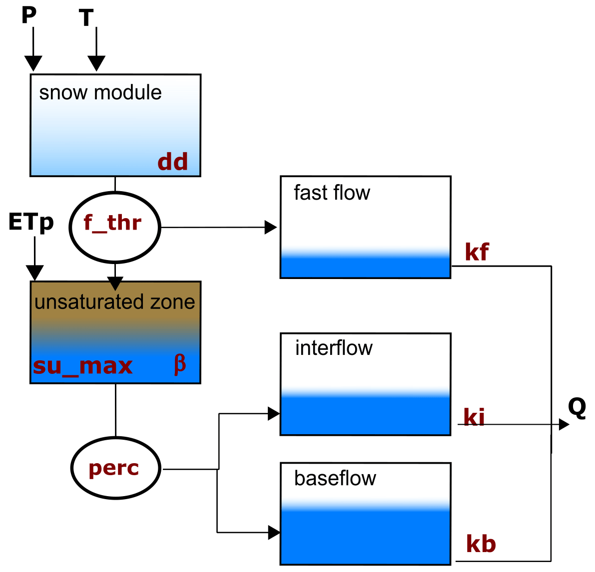
In this study, we employ a conceptual model named the Simple Hydrological Model (SHM) (Ehret et al., 2020) that is in its essence a slightly altered HBV model. A description of the model architecture and its internal working can be found in Appendix A. We used the SHM both as a stand-alone benchmark and as an integral component of the hybrid model.

To establish a benchmark for comparing our data-driven and hybrid methods, we performed individual calibrations of the SHM for each specific basin of interest. This approach is in line with Kratzert et al. (2019b, 2024) and Nearing et al. (2021), who indicate that conceptual models generally perform better when calibrated at the individual basin level rather than using a regional calibration approach. To ensure a fair comparison and mitigate potential calibration biases that may favor our hybrid model, we employed two established calibration methods and selected the one that yielded the best performance for each basin. We used “shuffled complex evolution” (SCE-UA) (Duan et al., 1994) and “differential evolution adaptive metropolis” (DREAM) (Vrugt, 2016), both implemented within the SPOTPY (Statistical Parameter Optimization Tool for Python) library (Houska et al., 2015).

2.4 LSTM

As mentioned in previous sections, we incorporated an LSTM model as a benchmark for our comparison. For a comprehensive understanding of the internal workings of LSTM networks, we refer to the work by Kratzert et al. (2018). In this subsection, we will provide an overview of the key aspects required to comprehend the training process. Our data-driven model was implemented using the PyTorch library (Paszke et al., 2019), and the corresponding code can be found in the repository accompanying this paper.

The model architecture and hyperparameters align with Lees et al. (2021) and Lees et al. (2022). We used a single LSTM layer with 64 hidden states, a dropout rate of 0.4, an initial learning rate of $\mathrm{1}\times {\mathrm{10}}^{-\mathrm{3}}$, and a sequence length of 365 d. The batch size was set to 256, and the initial bias of the forget gate was set to 3. Additionally, the Adam algorithm (Kingma and Ba, 2014) was used for the optimization.

We also maintained as input three dynamic forcing variables (precipitation, potential evapotranspiration, and temperature), along with the same 22 static attributes proposed in the original studies, which encode key characteristics of the catchments. The model output was compared against the observed specific discharge. Following common ML practices, both the input and output data were standardized using the global mean and standard deviation of the training dataset.

To train the LSTM, we used the basin-averaged Nash–Sutcliffe efficiency (NSE^*) loss function proposed by Kratzert et al. (2019b). This function divides the squared error between the modeled and observed output by the variance of the specific discharge series associated with each respective basin in the training period. As described by the authors, NSE^* provides an objective function that reduces bias towards large humid basins during the optimization process, avoiding the underperformance of the regional model in catchments with lower discharges. Given that we are training our regional model for a batch size N=256, the training loss was calculated according to Eq. (1):

$$\begin{array}{}\text{(1)}& {\mathrm{NSE}}^{*}={\displaystyle \frac{\mathrm{1}}{N}}\cdot \sum _{i=\mathrm{1}}^N{\displaystyle \frac{{\left(y_i^{\mathrm{obs}}-y_i^{\mathrm{sim}}\right)}^{\mathrm{2}}}{{\left(s_i+\mathit{ϵ}\right)}^{\mathrm{2}}}},\end{array}$$

where $y_i^{\mathrm{obs}}$ is the observed discharged (standardized), $y_i^{\mathrm{sim}}$ the simulated discharged (standardized), s_i the standard deviation of the flow series (in training period) for the basin associated with element i, and ϵ is a numerical stabilizer (ϵ=0.1) so that the loss function remains stable even when basins with low-flow standard deviations are considered.

2.5 Hybrid model: LSTM+SHM

Our hybrid model was created by combining an LSTM network, with the same architecture as the one from the previous section, with the SHM. The LSTM network predicts a set of values that serve as parameters for the SHM for each simulation time step. These parameter values are then utilized by the SHM to simulate the discharge, as indicated in Fig. 1.

Figure 1 Structure of the hybrid hydrological model: LSTM+SHM.

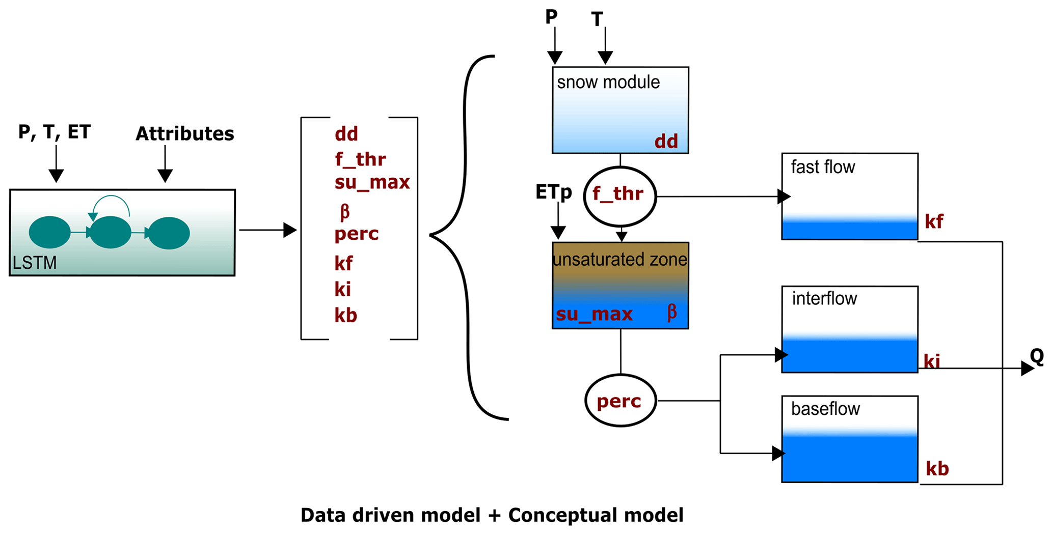
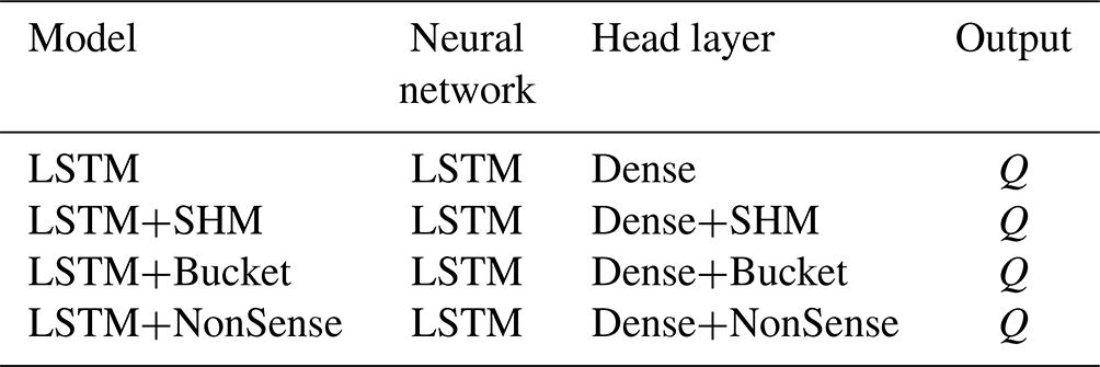
An alternative way to interpret the hybrid model is to see the conceptual model as a head layer on the LSTM. As we see in Table 1, in our stand-alone LSTM we require a dense layer (e.g., fully connected linear layer) to translate the information contained in the hidden states into a single output signal. In the LSTM+SHM case, a dense layer is still used to convert the hidden states into as many output signals as parameters in the conceptual model. However, these signals are further processed using the conceptual model to obtain the final discharge. One of the hypotheses that will be tested in the following sections is if further processing of the signals through the conceptual structure allows us to recover information about non-target variables, e.g., soil moisture.

Table 1 Visualization of hybrid models as head layers of data-driven methods.

Appendix B provides a comprehensive explanation of the training process for the hybrid models, emphasizing the distinctions from the training approach utilized for the LSTM models.

3 Results and discussion

3.1 Benchmarking our LSTM model

Kratzert et al. (2024) explains the importance of using community benchmarks to test if new ML pipelines are configured appropriately. They suggest that in the case that the researchers decide to use their own models or different setups, they should first recreate standard benchmarks to make sure that their model is up to date with the current state of the art and then make the respective changes.

Considering that the stand-alone LSTM model was going to be used as a baseline for all our experiments, we trained our LSTM model architecture on the benchmark established by Lees et al. (2021) for CAMELS-GB and compared its performance against their model. To further validate our architecture, we also trained on the benchmark established by Kratzert et al. (2019b) for CAMELS-US and again compared the performance of our model against theirs.

As we can see in Fig. 2, the cumulative distribution functions (CDFs) for the Nash–Sutcliffe efficiency (NSE) of the different basins are very much alike. For the case of Great Britain, Lees' model achieved a median NSE of 0.88, while ours reached 0.87. In the case of the USA, Kratzert's benchmark reported a median NSE of 0.759, while our model got 0.74. The small differences can be explained by the fact that both benchmark studies make the calculation based on an ensemble of various LSTM models, while we only presented the results for a single run. However, the overall agreement validates our model's pipeline and increases the confidence in the results.

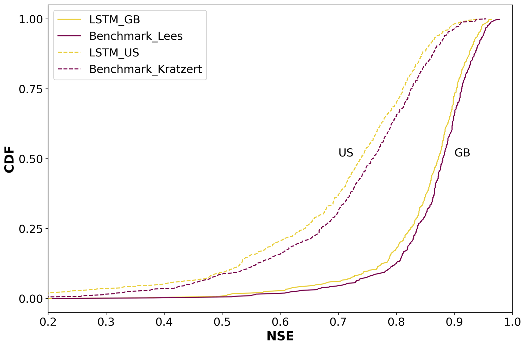
Figure 2 Cumulative density functions of the NSE comparing our LSTM model with current state-of-the-art benchmarks.

3.2 LSTM vs. LSTM+SHM

Once we tested our stand-alone LSTM pipeline, the next task was to develop our hybrid model (LSTM+SHM). By following the data and methods outlined in Sect. 2, we achieved a performance comparable to that of an LSTM. When evaluated across the 669 basins in the testing period, the LSTM reported a median NSE of 0.87, while the LSTM+SHM yielded a value of 0.84. Figure 3a displays a CDF–NSE curve, clearly demonstrating the close performance between both models. In the same figure, we can see that both models outperformed the basin-wide calibration of the SHM model, which achieved a median NSE of 0.76.

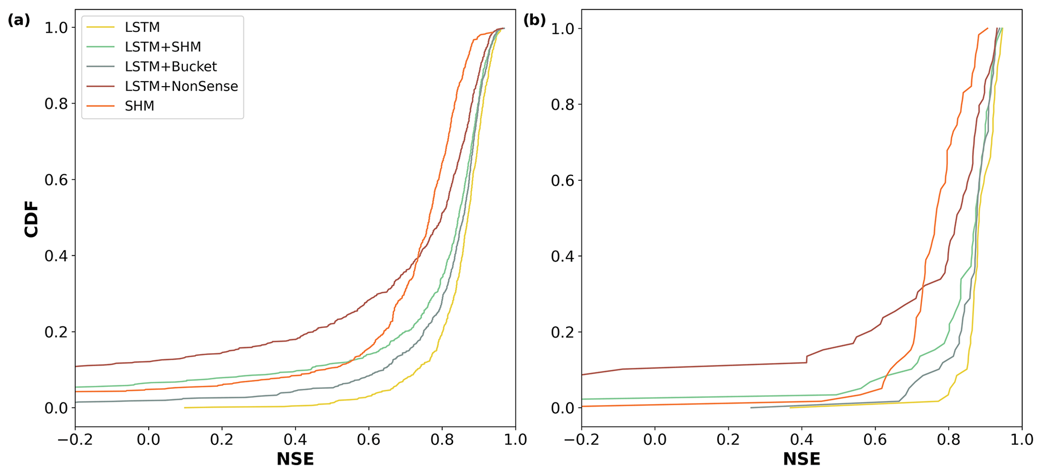
Figure 3 Cumulative density functions of the NSE for the different models. (a) CDF was calculated using all 669 basins; (b) CDF was calculated using a subset of 60 basins.

One point worth explaining is the decreased performance of our hybrid model compared to the LSTM in the low-performing basins. More specifically, the LSTM reported only 3 basins with NSE lower than zero, while the hybrid reported 44. Of these 44 basins, 37 were also the lowest-performing basins in the stand-alone SHM model, which suggests a problem with the input data. The LSTM network can account for biases in the forcing variables (e.g., precipitation or evapotranspiration) because mass conservation is not enforced (Frame et al., 2023). However, both the conceptual and the hybrid approaches have a mass conservative structure, so the input quantities cannot be adjusted. This problem was also reported by Feng et al. (2022) when applied to certain basins in CAMELS-US. It is important to highlight that this issue was observed in under 7 % ($\mathrm{44}/\mathrm{669}$) of the data, and in most cases, the performance of the hybrid approach is fully comparable with the LSTM.

In summary, we observed comparable performance between the LSTM and LSTM+SHM models. Moreover, both models outperformed the SHM-only model, which indicates that the dynamic parameterization given by the LSTM is able to improve the predictive capability of the model. This finding aligns with Feng et al. (2022), where they reached a similar conclusion despite using a different conceptual model and applying it to a different dataset. However, as described in the Introduction, we are interested in looking at the LSTM–SHM interaction to evaluate if the good performance of the hybrid model is due to the right reasons (Kirchner, 2006) and based on a consistent interaction between the two model approaches, or if the LSTM network is overwriting the conceptual element. This will be explored in the following section.

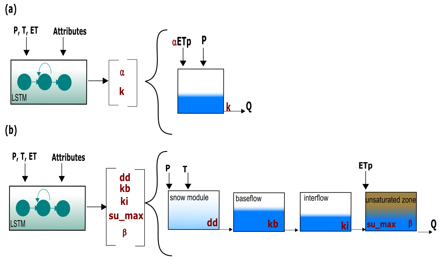
Figure 4 Structure of the different regularization mechanisms: (a) LSTM+Bucket; (b) LSTM+NonSense.

3.3 Effect of different regularization mechanisms

The first step to answer the aforementioned research question was to evaluate if the dynamic parameterization given by the LSTM can overcome the regularization imposed by the conceptual model. For this, we conducted two experiments, in which the structure of the conceptual model was modified. In the first experiment (see Fig. 4a), we substituted the SHM with a single linear reservoir, leading to the removal of most hydrological processes typically represented in a conceptual model through different reservoirs and interconnecting fluxes. A single bucket model only assures mass conservation and a dissipative effect in which the input is lagged based on the recession coefficient in combination with a macroscopic storage. As observed in Fig. 4a, the model involves two calibration parameters: the recession parameter k and a factor for the evapotranspiration term (α). Similar to the previous cases, we defined predefined ranges in which the parameters were allowed to vary, with k in the range [1–500] and α in the range [0–1.5]. Our initial expectation was that if our head layer (a) restricts the flexibility of the LSTM because the output of the LSTM (after our dense layer) is further passed through a one-process (single bucket) layer and (b) the one-process layer encodes almost no hydrological process understanding, then the performance of the model would drop. However this was not the case. The performance of this hybrid model (LSTM+Bucket) is fully comparable to that of the LSTM and LSTM+SHM, achieving a median NSE of 0.86 (see Fig. 3a). For reference, when calibrated without dynamic parameterization, the median NSE of the stand-alone bucket model drops to 0.59. This finding indicates that the LSTM's dynamic parameterization effectively compensates for the missing processes, and the regularization provided by the single bucket is insufficient to impact the model's performance.

Given the insights gained from the LSTM+Bucket experiment, we conducted a second experiment introducing an intentionally implausible structure in the conceptual model, referred to as LSTM+NonSense. As shown in Fig. 4b, we removed the fast-flow reservoir, creating a single flow path comprising the baseflow, interflow, and unsaturated zone, in that specific order. We also maintained the parameter ranges specified in Table B1, which restrict the baseflow reservoir to have smaller recession times than the interflow. Then, only after the water has been routed through these two reservoirs can it enter the unsaturated zone, where the outflow is no longer controlled by a recession parameter but by an exponential relationship depending on su_max and β. The stand-alone NonSense model yielded a median NSE of 0.51. However, after applying dynamic parameterization, the LSTM+NonSense achieved a median NSE of 0.80 (see Fig. 3a), improving the stand-alone NonSense by over 50 % and surpassing the SHM model in 60 % of the basins. During the test, we observed that the optimization routines tried to reduce the recession parameter of the baseflow and interflow to avoid the initial lagging. This caused the optimized parameters to reach the lower limits, which might have limited an additional performance increase. Expanding the parameter ranges might lead to a further performance gain; however, this would come at the cost of reducing the differences between the reservoirs, which contradicts the objective of the experiment. Taken together, these experiments provided valuable insights into addressing the first research question posed in the Introduction: can conceptual models effectively serve as a regularization mechanism for the dynamic parameterization given by the LSTMs? Based on our results, we observed that the regularization offered by the conceptual model is not strong enough to reduce the hybrid model performance, and the dynamic parameterization given by the LSTM can even compensate for missing processes and implausible structures. Figure 5 highlights that, for some basins, we obtained a similar hydrograph for all models used. Therefore, we recommend being careful about using this hybrid scheme for comparing different types of conceptual models or multiple working hypotheses (Clark et al., 2011), especially if we are evaluating model adequacy by performance alone, as the overall performance can be adjusted by the data-driven part.

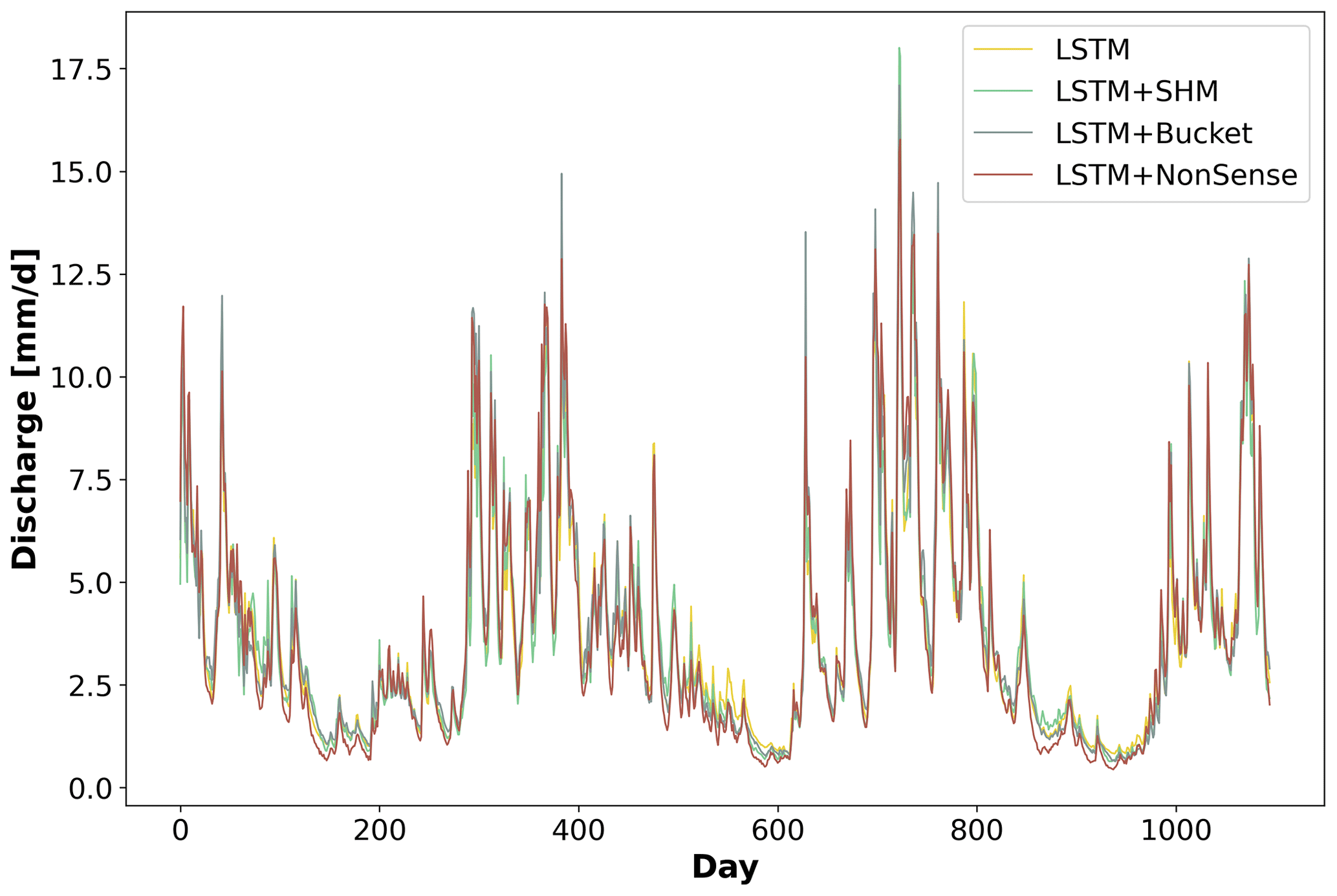
Figure 5 Specific discharge series in the testing period for basin ID 15006, simulated by the different models.

3.4 Testing on a subset of basins

In the above sections, we showed that both LSTMs and hybrid models outperformed stand-alone conceptual models. In this subsequent section, we replicate the experiments focusing on a subset of basins. This subset responded to an inherent limitation of conceptual models, which in principle does not affect data-driven techniques. Unlike LSTM networks, which learn directly from the data without a predefined structure, conceptual models have fixed model architectures designed to represent specific processes. This means that anthropogenic impacts such as reservoir operations, withdrawals, or transfers may not be adequately captured by conceptual models unless they are directly accounted for. While this limitation is a clear advantage of data-driven techniques, we wanted to make a comparison on a level playing field. Therefore, as a first filter, we selected only basins with the label “benchmark_catch=TRUE”, which, according to Coxon et al. (2020a), can be treated as “near-natural”, i.e., catchments in which the human influence in flow regimes is modest and where natural processes predominantly drive the flow regimes. As a second filter, we considered the temporal resolution of the data and the size of the catchment. The CAMELS-GB dataset contains data with a daily resolution. Consequently, we need to consider catchments with a sufficient size such that discharge variations are resolved by daily data. After applying the aforementioned filters, we identified 60 basins that passed both criteria. For detailed information on the specific basin IDs, please refer to the Supplement of this article.

Figure 3b shows the results when the models are tested on the subset of 60 basins. We can see that the LSTM (median NSE = 0.88), LSTM+SHM (0.87), LSTM+Bucket (0.88), and LSTM+NonSense (0.82) continue to outperform the stand-alone SHM (0.76) in a setting designed to account for the limitation of the latter. This result reaffirms the findings highlighted in the preceding sections.

3.5 Analysis of LSTM+SHM

To tackle our second research question and assess the interpretability of the conceptual part of our LSTM+SHM model, we conducted several tests. Hybrid models, as highlighted by Feng et al. (2022), Kraft et al. (2022), and Hoge et al. (2022), offer the advantage of providing access to untrained variables as the model's states and fluxes have dimensions and semantic meaning. As such, our first test was a model intercomparison. Specifically, we evaluated the filling level of the unsaturated zone reservoir, representing soil moisture in our model (LSTM+SHM), against ERA5-LAND soil water volume information. The process of utilizing reanalysis data and the necessary data processing steps for this comparison are detailed in Sect. 2.2.

Across the 669 basins in the testing period, the LSTM+SHM model demonstrated a median correlation of 0.86 when compared against the soil moisture simulation provided by ERA5-LAND. This result indicates that the unsaturated zone dynamics are well represented in our model and that the hybrid approach allows us to recover this variable without including any soil moisture information in our training.

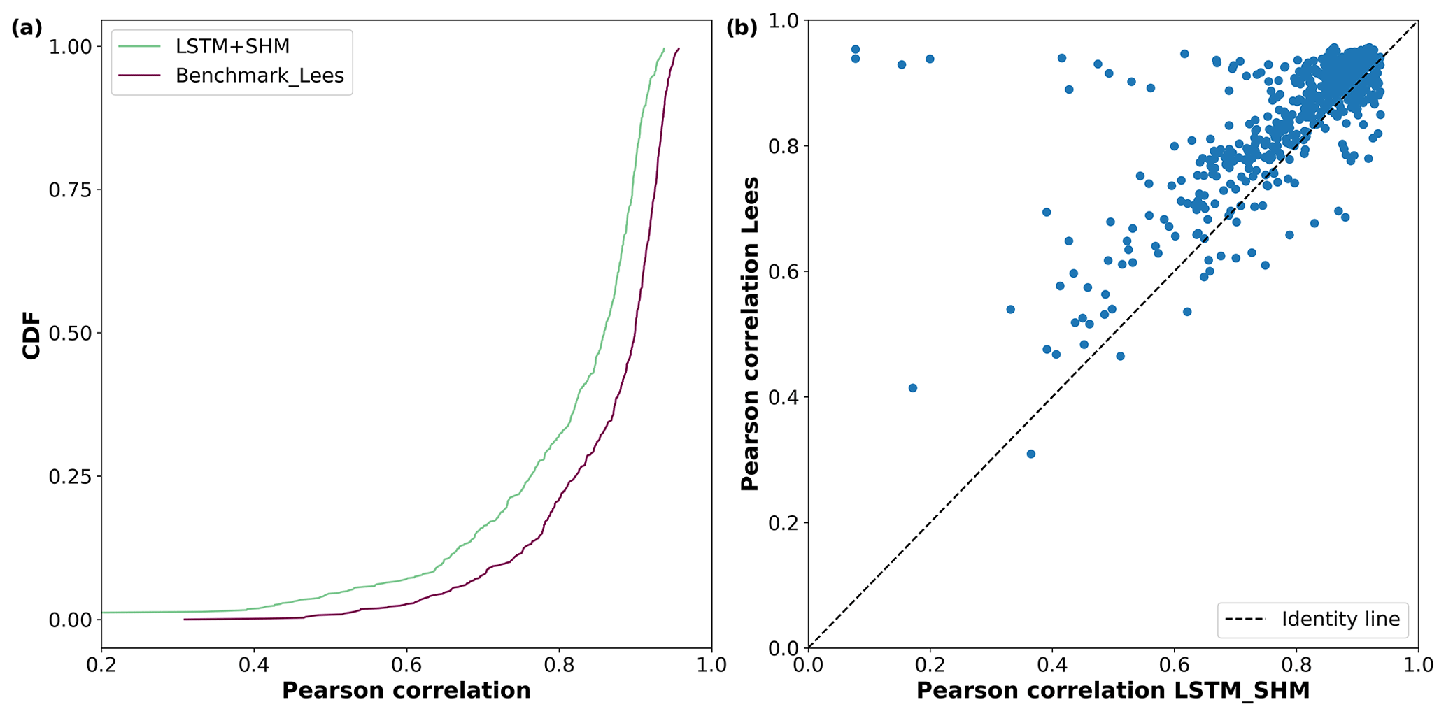
Figure 6 Comparison of soil moisture estimates using our hybrid approach method and the Lees et al. (2022) approach. The simulated results of both approaches were compared against ERA5-Land data. (a) CDF for the correlation coefficient obtained by both models when applied to the testing dataset; (b) comparison of correlations provided by both models.

Lees et al. (2022) present an alternative method to extract non-target variables from data-driven techniques. They train a model (which they call a probe) to map the information contained in the cell states of the LSTM to a given variable. Specifically, they trained an LSTM using CAMELS-GB, mapped the soil moisture information using a probe, and evaluated their outcome against ERA5-LAND data. Because our testing period was aligned with their experiment, we were able to directly compare their results to ours.

Lees' probe method reported a median correlation against ERA5-LAND data of 0.9, surpassing our value of 0.86. Figure 6 shows a more detailed comparison. Both methods got similar results in basins with high correlation; however, Lees' method was more robust in low-performing basins. This effect can be directly linked to the explanation we gave above when a similar behavior was observed when predicting discharge. The LSTM network can account for biases in the forcing variables because mass conservation is not enforced, while our hybrid approach is limited by their mass conservative structure.

The main difference with Lees et al. (2022) is that their probe to extract non-target variables needs to be trained, while in our hybrid approach no extra training needs to be done. The fact that in Lees et al. (2022) the probe can be as simple as a linear model, which requires few points to train, is not being argued, and in many cases, this will reduce the advantage given by our method.

Lastly, we would like to point out that the correlation obtained by the LSTM+Bucket (0.82) and LSTM+NonSense (0.85) models is still high, which can be attributed to the strong dependence of soil moisture with the precipitation and evapotranspiration series, both of which serve as boundary conditions for all models. This point also highlights our previously stated concern about using hybrid models for comparing different types of conceptual models or multiple working hypotheses.

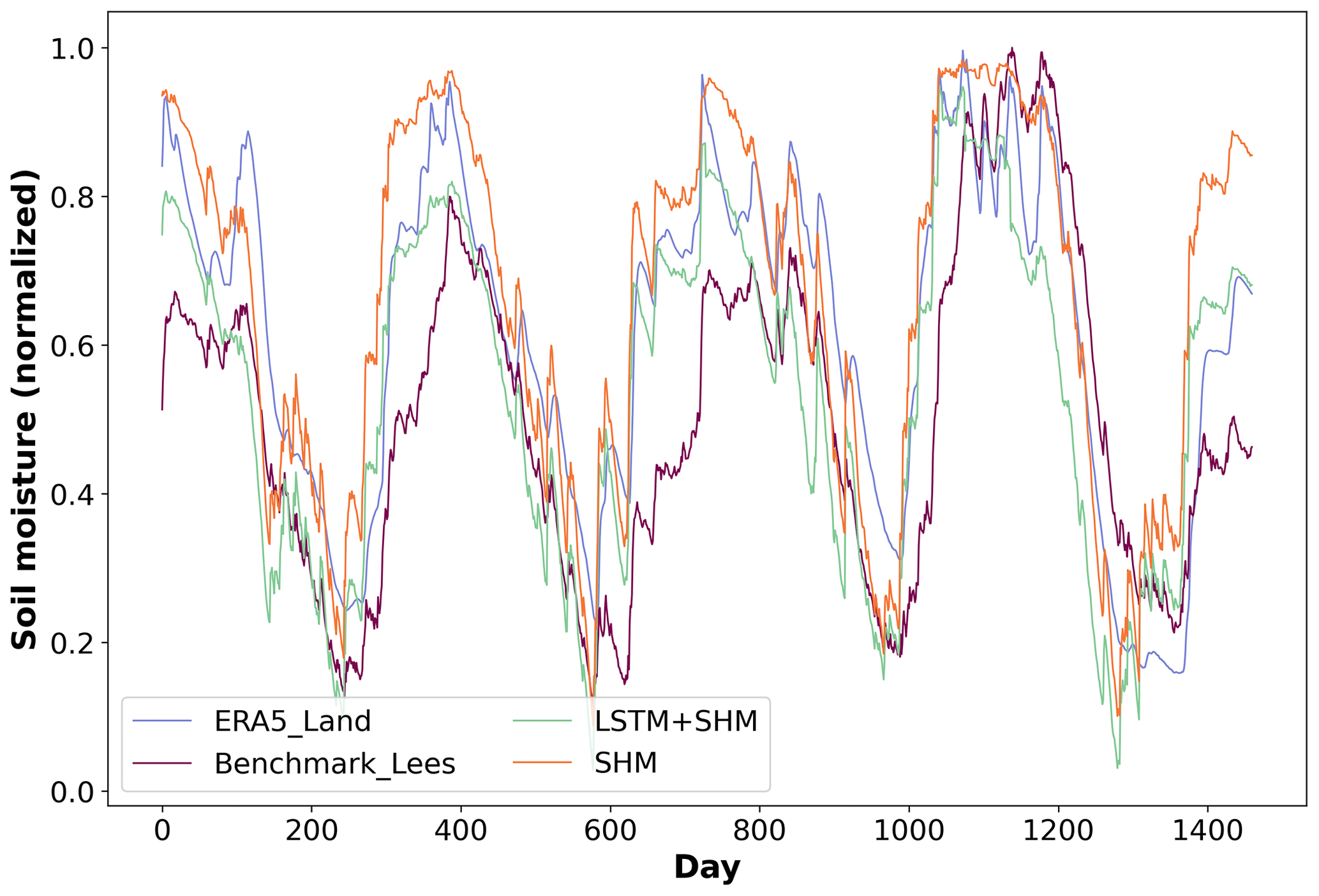
In addition to the comparison with external data, we also examined the correlation between soil moisture estimates produced by the LSTM+SHM model and the stand-alone SHM. The median correlation value of 0.96 further confirms that the unsaturated zone within our hybrid model operates under our initial expectations. Figure 7 exemplifies this agreement for basin 42010, where the modeled (LSTM+SHM) and ERA5-LAND series exhibit a correlation of 0.86, equivalent to the median correlation observed across all 669 basins. For reference, the median correlation of the stand-alone SHM over all basins was also 0.86.

Figure 7 Soil moisture time series comparison during the testing period for basin ID 42010.

The last experiment to further evaluate the consistency of our hybrid model was to analyze the parameter variation over time. Figure 8 presents the results for four calibration parameters: su_max, β, k_b, and k_i, across two different basins (reasons for choosing these two basins are explained below). We begin by examining the behavior of the first two parameters.

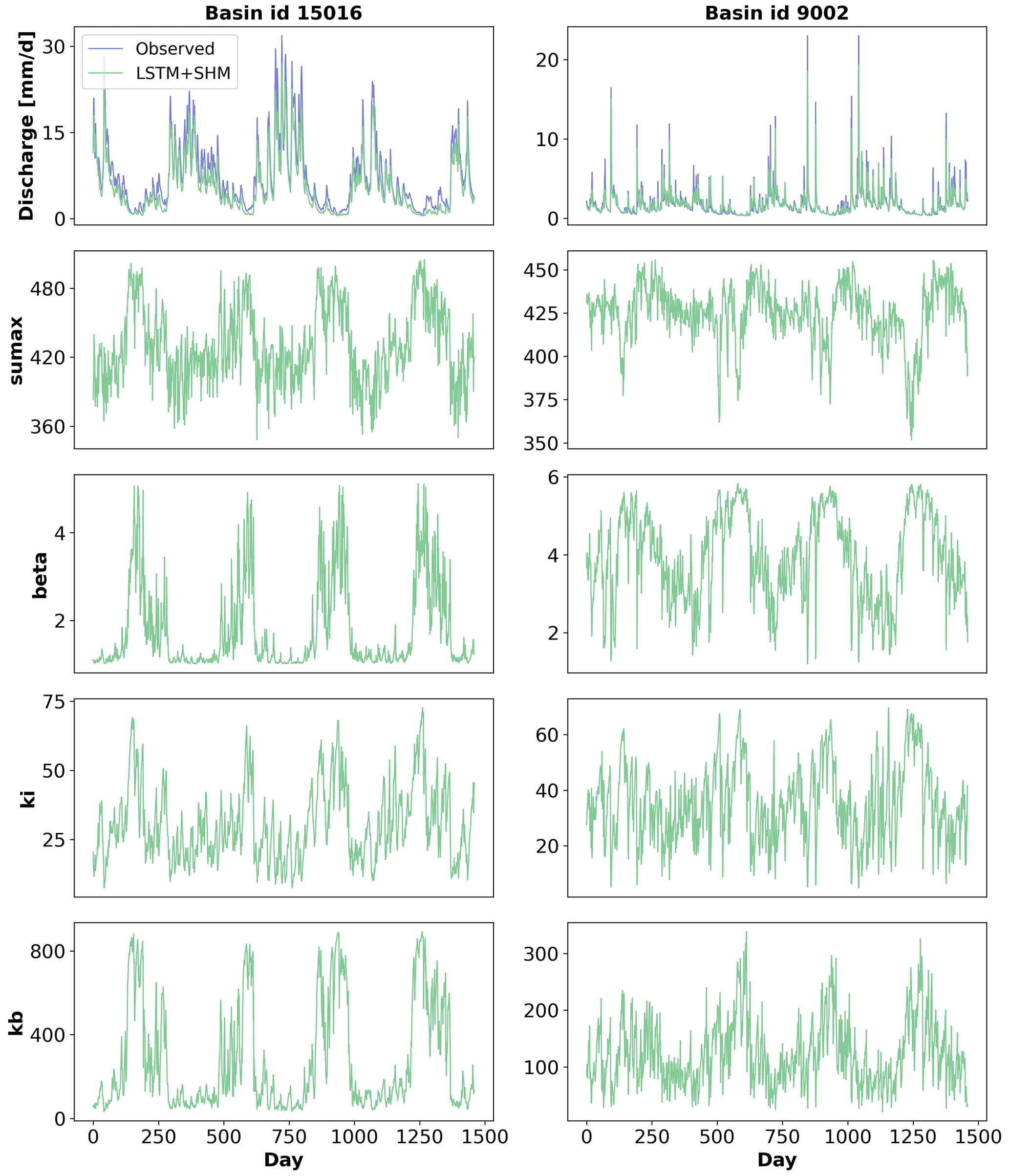
Figure 8 Time variation of parameters for basins 15016 (left column panels) and 9002 (right column panels). It should be noted that the y-axis ranges of the two basins differ.

The purpose of su_max and β is to control the water transfer from the unsaturated zone reservoir to the interflow and baseflow, following Eq. (2):

$$\begin{array}{}\text{(2)}& \mathrm{qu}\mathrm{\_}\mathrm{out}=\mathrm{qu}\mathrm{\_}\mathrm{in}\cdot {\left({\displaystyle \frac{\mathrm{su}}{\mathrm{su}\mathrm{\_}\max }}\right)}^{\mathit{\beta }},\end{array}$$

where qu_out represents the water going out of the unsaturated zone, qu_in represents the water entering the unsaturated zone from precipitation and snowmelt, su refers to the unsaturated zone storage or soil moisture, and su_max and β are the calibration parameters. It is important to note that the value of su cannot exceed su_max, which forces their quotient to be less or equal to one. Consequently, a larger value of su_max and/or β leads to a decrease in the unsaturated zone outflow.

The parameter variation in basin ID 15016 presents clear seasonal patterns. During low-flow periods, both parameters increase, resulting in reduced water availability for the remaining two reservoirs and, consequently, a decrease in the total outflow. On the other hand, during high-flow periods, the opposite happens. As both parameters decrease, there is an increase in water availability, resulting in higher outflows.

Regarding the other two parameters, k_b and k_i have a linear relationship with their respective outflows, acting as the denominator of their storage units $\left(q_{[i,b]}=\frac{s_{[i,b]}}{k_{[i,b]}}\right)$. For k_b, we can observe seasonal patterns, which allows the model to further increase the baseflow in wet periods and reduce it during dry seasons. This also aligns with our knowledge that hydraulic conductivity is lower when the soil is drier. On the contrary, k_i displays faster variations.

Basin 9002 shows high-frequency variability for most of the parameters but still a good agreement between the observed and simulated discharge. This basin also exhibits a large increase in performance when the dynamic parameterization is applied, achieving an NSE of 0.90 for the LSTM+SHM against an NSE of 0.73 for the stand-alone SHM. This boost in performance when the dynamic parameterization is applied is 4 times as high as the equivalent scenario for basin 15016. We argue that this is the basis for explaining the high-frequency variability we see in the figure.

In a hypothetical case in which we have a perfect conceptual model that considers all the processes happening in the basin, the predicted parameters will be constant. However, due to structural limitations of the conceptual architecture, the LSTM does take part in the predicting. Because of how the LSTM and the conceptual model are connected, the only way for the former to pass predicting information to the latter is through the parameters. Some deficiencies can be compensated with a more seasonal pattern, while others need faster pulses.

An alternative approach is to increase the complexity of our process-based part, reducing the necessity of the data-driven method to compensate for structural deficiencies. For example, Feng et al. (2022) represent the catchment processes using 16 HBV models acting in parallel, which are parameterized through an LSTM. In their case, the recession parameters were predicted as constant in time, and the necessary flexibility to get state-of-the-art performance and account for missing sub-processes was considered by the semi-distributed format.

It is worth considering that the bigger and more complex a process-based model is, the more similar it can become to an LSTM. More buckets generate higher flexibility, which can account for more complex process representation, such as different processes, multiple residence times, and mass transfers. Moreover, these buckets are normally updated considering some input and output fluxes and some losses. In an LSTM each cell state can be interpreted as a bucket, which can be modified by a forget gate, input gate, and (indirectly) output gate. The main difference is that the gates in the LSTM depend on the input and the previous hidden states, and in conceptual models, for simplicity, we usually take these as constants. However, this can be modified by making the gates of the buckets context dependent, and then both models would be alike. Therefore, regularizing a hybrid model with a complex conceptual model will probably reduce the work that needs to be done by the LSTM, but the final product will not be that different from having just a stand-alone LSTM.

4 Summary and conclusions

In recent years, the idea of creating hybrid models by combining data-driven techniques and conceptual models has gained popularity, aiming to combine the improved performance of the former with the interpretability of the latter. Following this line of thought, Feng et al. (2022) used as a hybrid approach the parameterization of a process-based hydrological model by an LSTM network. The authors demonstrated the potential of the technique to achieve comparable performance as purely data-driven techniques and to outperform stand-alone conceptual models. Kraft et al. (2022) also achieved promising results following a similar process.

Motivated by this outcome, our article dug into the effect of dynamic parameterization in our conceptual model and the consequences this might have on the interpretability of the model. More specifically, we tried to answer the following questions. (1) Do conceptual models effectively serve as a regularization mechanism for the dynamic parameterization given by the LSTMs? (2) Does the dynamic parameterization of the data-driven component overwrite the physical interpretability of the conceptual model?

The first step towards answering these questions was to create a hybrid model. We coupled an LSTM network with a conceptual hydrological model (SHM), using the former as a dynamic parameterization of the latter. In our study, we demonstrated that our hybrid approach (LSTM+SHM) was able to achieve state-of-the-art performance, comparable to purely data-driven techniques (LSTM). Both models were trained in a regional context, using the CAMELS-GB dataset. The median NSE of 0.87 and 0.84 for the LSTM and LSTM+SHM, respectively, outperform the basin-wise calibrated conceptual model, which served as the baseline and achieved a median NSE of 0.76. These findings align with existing literature. For instance, Feng et al. (2022) reached similar conclusions when applying a hybrid model to the CAMELS-US dataset.

Having accomplished a well-performing hybrid model, we addressed the first research question. By modifying the regularization given by the conceptual model, we tested to which degree the dynamic parameterization given by the LSTM has the potential to compensate for missing processes. We proved that a hybrid model composed of an LSTM plus a single bucket (LSTM+Bucket) was able to achieve a similar performance as the LSTM+SHM and LSTM-only models. This indicates that the regularization given by the conceptual model is not strong enough to drop the predictive capability of the hybrid model, and missing processes are outsourced to the data-driven part. We also demonstrated that if we use an intentionally implausible structure (LSTM+NonSense), the LSTM also has the flexibility to artificially increase performance.

However, the fact that the data-driven component possesses this capability does not necessarily imply that a well-structured conceptual model cannot be consistently utilized by the LSTM. Therefore, we further analyzed the internal functioning of our LSTM+SHM model to answer our second research question. We compared the soil moisture predicted by our hybrid model with data from ERA5-LAND. This test addressed one of the main benefits of hybrid models over purely data-driven ones, which is their ability to predict untrained states. Across our testing set, comprised of 669 basins, we obtained a median correlation of 0.86 between our simulated soil moisture and the ERA5-LAND data. This result indicates that our hybrid model was able to produce coherent temporal patterns of the untrained state variables, without having access to the corresponding data during the training period. We also compared the unsaturated zone reservoir of the LSTM+SHM against the unsaturated zone of the stand-alone SHM, which reported a median correlation of 0.96. These results indicate that the dynamic parameterization was operating the unsaturated zone reservoir consistently and according to our initial expectations. The last section of the study presented the results of the dynamic parameterization for two basins, where we showed that the high-frequency variations of the parameter's time series are caused by the LSTM trying to compensate for structural deficiencies in our process-based model.

We summarize the key findings of our study as follows:

1. Do conceptual models serve as an effective regularization mechanism for the dynamic parameterization of LSTMs?

   No. Our initial expectation was that if (a) our head layer restricts the flexibility of the LSTM and (b) the process layer encodes almost no hydrological understanding, then the performance of the model would drop; however, this was not the case. This indicates that structural deficiencies in the architectures can be compensated by the data-driven part. Therefore, we recommend being careful about using this hybrid scheme for comparing different types of process-based models, especially if we are evaluating model adequacy by performance alone, as the overall performance can be adjusted by the data-driven part.

2. Does the data-driven dynamic parameterization compromise the physical interpretability of the conceptual model?

   Partially. We showed that a well-structured conceptual model maintains certain interpretability and even gives us access to untrained variables. However, we also showed that even with a well-structured conceptual model, the LSTM is going to compensate for missing processes and structural limitations, especially when the architecture of the process is not well suited for a specific case. Increasing the complexity of the process-based model would result in less intervention of the data-driven part; however, we argue that the more complex a process-based model is, the more similar it will be to an LSTM network.

3. To bucket or not to bucket?

   In our experiments, we were not able to increase the performance of the data-driven models by adding a conceptual head layer, and even though the mean performance of the different models was the same, purely data-driven methods showed better results in low-performing basins. Therefore, until this point, the remaining advantage is the access to non-target variables, which other authors have accomplished with the use of probes. In future research, we will conduct other experiments to evaluate the performance of hybrid models under different conditions, but until this point, we do not have evidence that adding buckets gives a considerable advantage over purely data-driven techniques.

Appendix A: SHM model

In this section, we offer a concise overview of the conceptual model's key features. For a fully detailed explanation, we refer to Ehret et al. (2020). In a slight variation from the original paper, we included a snow module, and the potential evapotranspiration is read directly from the CAMELS-GB dataset.

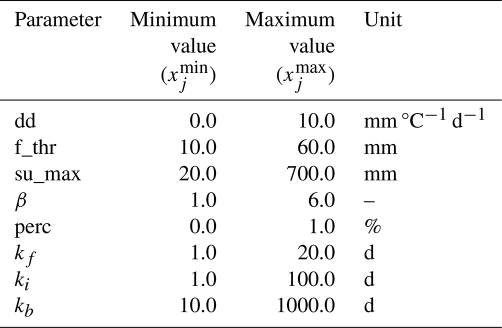
Figure A1 illustrates the overall structure of the model. The model input consists of three forcing variables: precipitation (P) [mm d⁻¹], temperature (T) [°C], and potential evapotranspiration (ET_p) [mm d⁻¹]. These three quantities were read directly from the CAMELS-GB dataset (Coxon et al., 2020a). To emulate the hydrological processes occurring in the basin, the model uses five storage components, namely, snow module, unsaturated zone, fast flow, interflow, and baseflow. Overall, to regulate the fluxes between components, eight parameters need to be calibrated: dd, f_thr, su_max, β, perc, k_f, k_i, and k_b (see units in Table B1).

The snow module receives P and T as inputs. Based on the temperature, precipitation is either stored as snow or moves forward together with additional discharge from snowmelt (if any). Snowmelt is calculated using the degree-day method in which the parameter dd relates to the volume of snowmelt at a given temperature. If the outflow of the snow module exceeds a threshold (f_thr), the excess is directed to the fast-flow reservoir, while the remaining portion enters the unsaturated zone bucket. On the other hand, if the snow storage outflow is smaller than f_thr, all water enters the unsaturated zone as input. Within the unsaturated zone, several processes occur. First, evapotranspiration causes water loss. The potential evapotranspiration (ET_p) is provided as a forcing variable but is adjusted to reflect the actual evapotranspiration considering water availability. Additionally, there is an outflow from the unsaturated zone, determined by a power relationship involving the parameters su_max and β. This outflow is then divided by the perc parameter, allocating portions to the inflows of the interflow and baseflow storages. Finally, the total discharge of the basin is computed as the sum of the outflows from the fast-flow, interflow, and baseflow storages. Each outflow is a linear function of its corresponding storage and the recession parameters k_f, ki, and k_b, respectively.

Figure A1 Structure of the SHM hydrological model used for rainfall–runoff prediction.

Appendix B: Training process comparison between hybrid and LSTM models

While the coupling of the data-driven and conceptual models may appear straightforward from a general perspective, it is important to highlight several details. First, as one can notice from Fig. 1 in the main paper, the forcing variables (P, T, ET) are used as inputs for both the LSTM and the SHM. The forcing variables and static attributes used as inputs for the LSTM are standardized using the method described in the previous section. However, due to the mass-conservative structure of the SHM, their input variables (P, T, ET) are used in the original scale. Second, it is important to consider that the SHM parameters have certain feasible ranges. While the LSTM could theoretically learn these ranges, the optimization process becomes highly challenging due to the immense search space involved. We found that without constraining the parameter ranges, the LSTM was not able to identify parameters that yield a functional hydrological model. Hence, we predefined ranges within which the parameters can vary (see Table B1). These ranges were defined considering the findings in Beck et al. (2016, 2020), which provide valuable insights into the appropriate parameter values of conceptual models. By defining these ranges, we not only reduced the computational costs of the optimization but also ensured consistency with the methodology employed by Feng et al. (2022).

To map the output of the LSTM network to the predefined ranges, the j outputs (j=8, one per parameter) are passed through a sigmoid layer to transform the values to a [0, 1] interval. Then the transformed values are mapped to the predefined ranges through a min–max transformation, as exemplified in Eq. (B1):

$$\begin{array}{}\text{(B1)}& {\mathit{\theta }}_j=x_j^{\min }+\mathrm{sigmoid}\left(o_j\right)\cdot \left(x_j^{\max }-x_j^{\min }\right),\end{array}$$

where θ_j is each of the values passed as parameters to the SHM, o_j are the original outputs of the LSTM network, and $x_j^{\min }$ and $x_j^{\max }$ correspond to the minimum and maximum values of the predefined ranges (see Table B1) in which each parameter can vary, respectively.

Table B1 Search range for SHM parameters during hybrid model optimization.

mm: millimeters; °C: degrees Celsius; d: days.

Lastly, there is a difference in how we trained our LSTM and hybrid model. The first one was trained using a seq2one approach, while the second one used a seq2seq methodology. Furthermore, even though both models used a spin-up period (e.g., sequence length), the spin-up period of the hybrid model also considered a time to stabilize the internal states of the conceptual model.

To facilitate the understanding of the previous concepts, let us create an example. Let us assume that both the LSTM and the hybrid model were trained on 60 basins and 10 years (∼3652 d) of data, even though we know from before that this was not the case.

For training the LSTM, we use a batch size of N=256 and a seq2one method. Therefore, to construct each batch we randomly select, without replacement, 256 data points from the total pool of $\mathrm{3652}\cdot \mathrm{60}=\mathrm{219}\mathrm{120}$ training points. For each of the 256 points of our batch, we run our LSTM for a given sequence length (e.g., 365 time steps) and extract the last simulated value. We then calculate our loss function with a metric that quantifies the difference between the observed and simulated values of the 256 training points and backpropagate this loss to update the network weights and biases. To complete an epoch, we iterate through the $\frac{\mathrm{219}\mathrm{120}}{\mathrm{256}}=\mathrm{855}$ batches.

In the case of the hybrid model, we train it as a seq2seq approach; therefore, to calculate the loss function we do not just use the last element of our simulated sequence but a part of that sequence (e.g., 365 time steps). Therefore, for the same scenario of 60 basins and 10 years of data, we have $\frac{\mathrm{60}\cdot \mathrm{10}\cdot \mathrm{365}}{\mathrm{365}}=\mathrm{600}$ training vectors, each with 365 elements that are used to calculate the loss. If we use a batch size of N=8, each batch will contain 8 randomly selected vectors with 365 sequential training points each, so the loss function will quantify the difference of $\mathrm{365}\cdot \mathrm{8}=\mathrm{2920}$ simulated and observed values. To complete an epoch, we iterate through $\frac{\mathrm{600}}{\mathrm{8}}=\mathrm{75}$ batches.

The other small difference while training the models is the length of the spin-up period. For the LSTM, we use a sequence length of 365 d, which means that we run a sequence of 365 d and extract the last value of this sequence to calculate the loss. The first 364 d help us consider the historical information to make a good prediction and to avoid bias due to the initialization of the cell states (usually zero). In our hybrid model, the LSTM uses a sequence length of 180 d, which means that only after 180 d do we start to retrieve the parameters that go into the conceptual model. The purpose of these 180 d is the same as before, consider the historical information to make a context-informed parameter estimation and avoid the bias due to the initialization of the cell states. However, we also need a warm-up period to avoid a biased result due to the initialization of the different storages of the conceptual part. Therefore, for each instance of the batch, we ran our conceptual model for a 2-year period. The initial year serves solely as a warm-up period (excluded from the loss function), while the second year's data are utilized for actual training. Figure B1 illustrates the data handling while training both models.

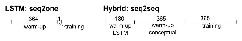
Figure B1 Training scheme comparison for LSTM and hybrid model. The former one uses a seq2one approach. The latter uses a seq2seq approach, and the total spin-up period consists of a sequence length for the data-driven part plus a warm-up period for the states of the conceptual part.