the Creative Commons Attribution 4.0 License.
the Creative Commons Attribution 4.0 License.
 | 04 Jun 2024
Investigation of the functional relationship between antecedent rainfall and the probability of debris flow occurrence in Jiangjia Gully, China
Shaojie Zhang
Xiaohu Lei
Hongjuan Yang
Juan Ma
Dunlong Liu
Fanqiang Wei
A larger antecedent effective precipitation (AEP) indicates a higher probability of a debris flow (Pdf) being triggered by subsequent rainfall. Scientific topics surrounding this qualitative conclusion that can be raised include what kinds of variation rules they follow and whether there is a boundary limit. To answer these questions, Jiangjia Gully in Dongchuan, Yunnan Province, China, is chosen as the study area, and numerical calculation, a rainfall scenario simulation, and the Monte Carlo integration method have been used to calculate the occurrence probability of debris flow under different AEP conditions and derive the functional relationship between Pdf and AEP. The relationship between Pdf and AEP can be quantified by a piecewise function. Pdf is equal to 15.88 %, even when AEP reaches 85 mm, indicating that debris flow by nature has an extremely small probability compared to the rainfall frequency. Data from 1094 rainfall events and 37 historical debris flow events are collected to verify the reasonability of the functional relationship. The results indicate that the piecewise functions are highly correlated with the observation results. Our study confirms the correctness of the qualitative description of the relationship between AEP and Pdf, clarifies that debris flow is a small-probability event compared to rainfall frequency, and quantitatively reveals the evolution law of debris flow occurrence probability with AEP. All the above discoveries can provide a clear reference for the early warning of debris flows.
- Article
(1196 KB) - Full-text XML
-
Supplement
(470 KB) - BibTeX
- EndNote


Antecedent effective precipitation (AEP) is likened to a Trojan horse lurking inside a loose soil mass, which can cooperate with subsequent rainfall at any time to trigger debris flow in a debris flow gully. AEP is equivalent to the precipitation preserved in soil mass before the triggering rainfall process; it represents the saturation degree of loose soil mass (Segoni et al., 2018). Therefore, the soil moisture that has accumulated from antecedent rainfall since the beginning of a rainfall season has a significant influence on how new storm rainfall interacts with the loose soil mass within a gully (Fiorillo and Wilson, 2004; Long et al., 2020). The increase in AEP can decrease the shear strength of a loose solid material provided by shallow landslides or channel erosion (Papa et al., 2013; Senthilkumar et al., 2017; Liu et al., 2020), and, as a consequence, the supply rate of solid material resources can be significantly enhanced in the subsequent rainfall process (Wei et al., 2008; Bennett et al., 2014; Zhang et al., 2020). Additionally, increased AEP and moisture content have been shown to enhance rainfall-induced surface runoff in a variety of environments (Tisdall, 1951; Luk, 1985; Le Bissonnais et al., 1995; Castillo et al., 2003; Jones et al., 2017; Hirschberg et al., 2021). Thus, AEP plays an important role in the formation of debris flows (Hong et al., 2018).
Rainfall thresholds represent the difficulty degree of debris flow triggered by rainfall (Marra et al., 2017). Investigations including the influence of AEP on the rainfall threshold can be helpful in examining the relationship between AEP and debris flow occurrence. Currently, the relationship between AEP and the rainfall threshold indicates that there is a negative correlation between AEP and rainfall conditions that trigger debris flows (Huang, 2013). AEP also represents the saturation degree of loose soil mass (Zhao et al., 2019a; Abraham et al., 2021), and integrating soil moisture with rainfall thresholds has been proven effective in improving prediction performance (Segoni et al., 2018; Zhao et al., 2019b; Abraham et al., 2020). Scholars also have attempted to analyze the influence of antecedent soil moisture on the rainfall threshold triggering debris flow (Cui et al., 2007; Hu et al., 2015), and there is still a negative correlation between antecedent soil moisture and triggering rainfall conditions (Chen et al., 2017), just like the relationship between AEP and the rainfall threshold. The above investigations show that an increase in AEP can significantly decrease the rainfall conditions for triggering a debris flow, which in turn means that debris flow is more likely to occur. Generally, the qualitative description of “the greater the AEP, the higher the probability (Pdf) of subsequent rainfall triggering the debris flow” (De Vita et al., 2000; Bel et al., 2017) has gradually become a consensus. Therefore, discovering a specific function to describe this qualitative description is helpful in further demonstrating the above consensus, revealing a certain evolutionary law of debris flow with rainfall in nature.
To quantify the evolution law of Pdf with the changing AEP, a numerical model denoted as the “Dens-ID” can correlate the rainfall parameters (I and D) with the debris flow density (Zhang et al., 2020; Long et al., 2020; Zhang et al., 2023), and it has been used to construct the rainfall intensity–duration (ID) threshold curves under different AEP conditions. The ID threshold curves with upper and lower bounds can delineate the closed region in the ID coordinate system, which represents the set of all rainfall conditions that can trigger debris flow at a certain AEP. Consequently, the probability of natural rainfall falling into a closed region is equivalent to Pdf, which can then be calculated based on Monte Carlo integration. The next section introduces the basic information of study area including the rainfall and debris flow event data collected from the study area. The third section addresses how to establish the functional relationship between the AEP and Pdf using the Dens-ID and Monte Carlo integration method. Sections 4, 5, and 6 discuss the results and state the conclusions of this study.
The Jiangjia Gully (JJG) is a primary tributary of the Xiaojiang River, which is located in the Dongchuan District of Kunming, Yunnan Province, China (Fig. 1). As shown in Fig. 1, JJG has a drainage area of 48.6 km2, with elevations ranging from 1040 to 3260 m. In this gully, the relative relief from the ridge to the valley reaches 500 m, and most of the slope gradient is greater than 25°. Slopes within JJG are covered by abundant loose soil with a thickness of more than 10 m. Shallow landslides are frequently triggered by intense rainfall processes in JJG, providing a large number of solid materials for debris flow (Yang et al., 2022). Before 1979, the Menqian and Duozhao gullies were the two main tributaries of JJG, accounting for 64.7 % of the entire drainage area. The upstream areas of the two main tributaries are the initiation zones of the debris flows, and the channels of the upstream tributaries are narrow and V-shaped (Zhang et al., 2020). However, several check dams have been constructed in Duozhao Gully since 1979, which have significantly reduced debris flow activity in this sub-gully (Zeng et al., 2009). Currently, Menqian Gully with an area of 13.2 km2 is the primary source area. The slope gradient of its both sides is very steep; i.e., the mean slope in Menqian Gully is 32°, and the maximum slope can reach 70°. Bedrock that mainly consists of slates formed in lower Proterozoic crops out in the unvegetated or sparsely vegetated lower part. The bedrock is fragmented and mostly disintegrates into clasts with the size more than 20 mm. The upper part of the bedrock is lain by soil mantles with thicknesses of 0.5–20 m, which are covered by grasses and shrubs or are used for terrace farming. The soil mantle is poorly sorted and composed of particles from clay to boulder. The translational zone from the upper to the lower parts of the slope is prone to shallow landslides. Some landslides directly evolve into debris flows, while the others release sediment to the channel, which is mobilized by runoff in debris flow events (Yang et al., 2022).
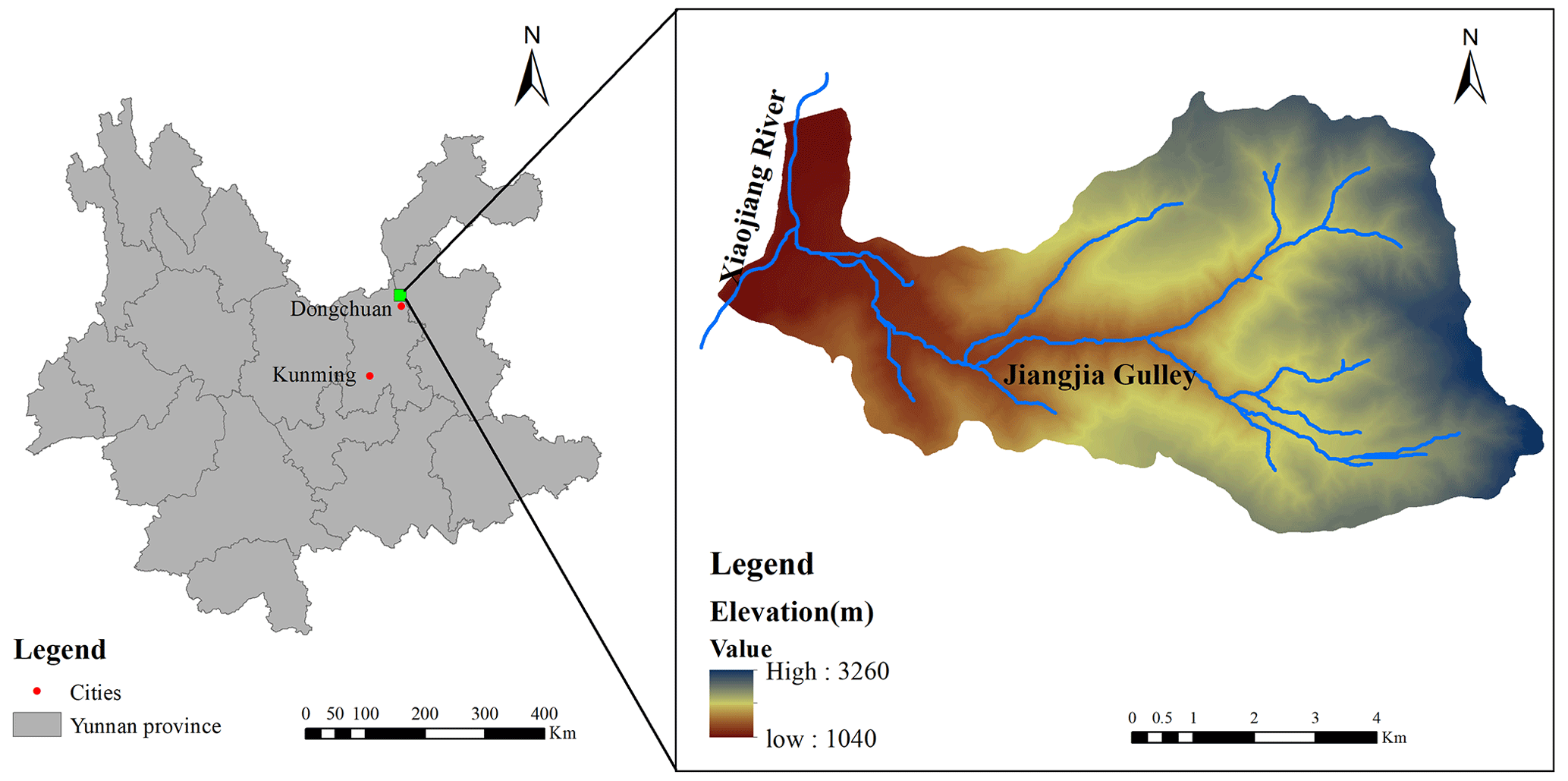
Figure 1Location of JJG.
Steep terrain provides a beneficial potential energy condition for transporting a large amount of loose solid materials from JJG to Xiaojiang River. Consequently, debris flows in JJG can be easily triggered by high-intensity rainstorm or long-duration rainfall processes (Zhang et al., 2020). The solid material necessary for a debris flow in a gully may be from shallow landslides (Iverson et al., 1997; Gabet and Mudd, 2006; Zhang et al., 2020; Long et al., 2020) or runoff-induced bed erosion (Berti and Simoni, 2005; Coe et al., 2008; Tang et al., 2020; Bernard and Gregoretti, 2021). In JJG, shallow landslides are the main sources for the solid material supply (Zhang et al., 2014; Liu et al., 2016; Yang et al., 2022), which is consistent with the assumptions of Dens-ID (Zhang et al., 2020). Thus, JJG is used as the study zone for deriving the function that describes the relationship between AEP and Pdf.
3.1 Dens-ID
Debris flow gullies characterized by a solid source supply from landslides are widely distributed in southwest China (Zhang et al., 2014). For this type of debris flow gully, our previous study proposed Dens-ID, aiming at correlating debris flow density to rainfall parameters based on a water–soil coupling mechanism (Zhang et al., 2020; Long et al., 2020). Den-ID assumes debris flow to be a water–soil mixture. It contains three core simulating contents: hydrological simulation, water–soil coupling to calculate the water–soil mixture density, and the correlation of density to rainfall parameters.
-
Simulating hydrological processes. The purpose is to provide parameters for estimating rainfall-induced runoff and the supply volume of rainfall-induced loose solid materials. Based on the digital elevation model (DEM) of a gully, Den-ID can simulate the rainfall-induced runoff and water diffusion in the vertical direction within the soil mass. The rainfall infiltration border is controlled by Eq. (1).
where θ is the soil water content; , which represents the soil water diffusivity; z is the soil depth, which is positive downwards along the soil depth as the topsoil is taken as the origin point; K(θ) is the hydraulic conductivity; I(t) is the rainfall intensity; and ψ is the soil matrix suction. When the rainfall intensity is less than the surface infiltration capacity, Eq. (1) is used to represent this physical process, whereas the case of precipitation intensity exceeding the infiltration capacity of topsoil means that the surface is saturated, and the excess precipitation from the topsoil is converted into runoff. Therefore, the pressure infiltration of each grid cell is not considered.
Equation (2) is the Richard differential infiltration equation (Richards, 1931), which is used to describe the water movement along the vertical direction within soil mass after precipitation infiltrates into topsoil. Dens-ID uses the finite-difference method to solve Eqs. (1) and (2) and can provide the runoff depth (denoted as dw(i,t)), soil water content, and soil matrix suction for each grid cell. Dens-ID then calculates the runoff volume using runoff depth dw(i, t) in Eq. (3).
where n represents the total number of grid cells that can generate runoff at time t, Vw(t) represents the total volume of runoff within a gully at time t, Sg represents the area of the grid cell generating runoff, and T represents the total duration of a rainfall process.
-
Calculating supply amount of loose solid materials and density of the water–soil mixture. Taking hydrological parameters such as soil water content and soil matrix suction as inputs, Dens-ID uses Eqs. (4) and (5) to estimate the supply amount of rainfall-induced loose solid materials within a gully. Equation (4) calculates safety factor Fs of each grid cell as a function of the matrix suction and soil moisture. Fs > 1 indicates that the grid cell is stable and cannot supply solid material to the gully, whereas a grid with Fs < 1 can provide solid material in the form of a shallow landslide.
where Fs represents the safety factor of each grid cell; c is the soil cohesion force; φ is the internal friction angle; φb is related to the matrix suction and is approximately equal to φ as the low matrix suction is small; ds is the soil depth; and ψ is the matrix suction, which is a function of soil water content and can be described by the Van Genuchten model (Van Genuchten, 1980).
Equation (4) is used to estimate the total volume of solid materials from all the unstable grid cells during a rainfall process.
where m represents the number of grid cells that can provide solid material at time t, and Vs(t) is the total volume of solid material within a gully at timet. At time t, the density of the water–soil mixture after full coupling between runoff and solid material can be calculated using Eq. (6).
where ρmix(t) is the density of the water–soil mixture; ρw is the water density; ρs is the density of the soil particles; and Vmix(t) is the volume of the water–soil mixture, which is the sum of Vw(t) and Vs(t). Vw(t) and Vs(t) are the key variables that can be derived using Eqs. (3) and (5).
-
Correlating density to rainfall parameters including rainfall intensity and duration. After firstly presetting the density of the water–soil mixture as ρmix, Dens-ID also needs to simulate many rainfall scenarios including long durations with low-intensity rainfall and short durations with high-intensity rainfall in order to obtain a sufficient number of [Di, li]. Using each [Di, Ii] as input, Dens-ID then can calculate the density using Eq. (6). If the calculated density is equal to ρmix, the [Di, Ii] combination is saved by Dens-ID. After Dens-ID completes the trial calculations, all combination data of [Di, Ii] that satisfy the constraints of the preset density (ρmix) can be collected as a dataset. Each collected [Di, Ii] within the dataset corresponds to the preset ρmix. Accordingly, Dens-ID can correlate rainfall parameters (D and I) to debris flow density (Long et al., 2020). Dens-ID can derive ID threshold curves by fitting the selected [Di, Ii] data, and each ID curve corresponds to a debris flow density value (Zhang et al., 2020). As the density of debris flow in JJG varies in a specific interval of 1.2–2.3 g cm−3 (Zhang et al., 2014; Zhuang et al., 2015; Long et al., 2020), the threshold curve that corresponds to the boundary value can form a closed area with the I and D axes in the ID coordinate system. The case of monitoring or forecasting rainfall falling into this closed area indicates that the rainfall condition may trigger debris flow. The verification results in JJG show that Dens-ID can effectively describe the mechanism and process of debris flow formation, and its prediction accuracy is approximately 80.5 %, which is 27.7 % higher than that of statistical models (Zhang et al., 2020). Such a high prediction accuracy can further indicate that the closed area formed by the derived ID curves has a very reasonable location and coverage in the ID coordinate system, providing extremely reliable analytical data in this study.
3.2 JJG data for model Dens-ID
The JJG datasets for Dens-ID are terrain data, hydrological parameters, and soil mechanical parameters. The DEM is the basal data for deriving other terrain data, including slope length, gradient, and river channels; the spatial resolution of the DEM is 0.5 m, and a DEM with a grid size of 10 m was generated using the resampling technology in ArcGIS. The hydrological parameters are related to the soil types within JJG; the five key parameters are the saturated soil water content, residual soil water content, the two parameters of soil water characteristic curve including n and m, and the infiltration rate of topsoil. The soil mechanical parameters are the soil cohesion force and internal friction angle obtained through direct shear tests on the soil samples. Detailed data are available in Zhang et al. (2020) and Long et al. (2020).
3.3 Historical rainfall and debris flow data
Rainfall data for the rainy seasons between 2006 and 2020 have been collected from the JJG observation station, and it is necessary to identify each rainfall process from the long-term rainfall sequences. Inter-event time (IET) is defined as the minimum time interval between two consecutive rainfall pulses (Adams et al., 1986). IET has a strong influence on the rainfall event starting and ending times (Bel et al., 2017), and Peres and Cancelliere al. (2018) have identified that IET depends on whether the mean daily potential evapotranspiration (MDPE) is larger than precipitation within the IET. The long observation of evaporation within JJG showed that MDPE is about 4 mm; precipitation during IET > 0.5 mm is considered the end of a rainfall process. Under this standard, 1094 rainfall events and 37 debris flow events were identified during the sampling period. Detailed rainfall data information can be found in Table S1 in the Supplement. The AEP listed in Table S1 is considered the weighted sum of the rainfall periods before the occurrence of debris flow (Long et al., 2020), and it can be calculated using Eq. (7).
where AEP is the antecedent effective rainfall; K is the attenuation coefficient, which is equal to 0.78 based on the field test in JJG (Zhang et al., 2020); and n is the number of days preceding the debris flow occurrence.
Based on the observed rainfall data, the 1094 AEP events are calculated using Eq. (7) and listed in Table S1. The AEP corresponding to each rainfall event varies from 0–88 mm. Taking this variation range as a reference, the variation range of the AEP input in the Dens-ID model is set between 10 and 85 mm. Since AEP in JJG ranges from 0–88 mm according to the measured rainfall data, Dens-ID presets several AEP values including 10, 15, 20, 25, 30, 35, 40, 45, 50, 55, 60, 65, 70, 75, 80, and 85. The cases of AEP = 0 and AEP = 5 mm are excluded, because the two cases represents such a low initial rainfall condition that any ID curve cannot be derived from Dens-ID. The purpose of increasing AEP by an interval of size 5 is to get adequate ID curves, which will be helpful to calculate Pdf under different AEP conditions.
3.4 Monte Carlo method for calculating the definite integral
Because of the boundary of the debris flow density in JJG (1.2–2.3 g cm−3), Dens-ID produces the corresponding upper and lower boundary curves under a specific AEP condition. The two boundary curves can be described using a power function.
These two threshold curves can delineate an enclosed area in the ID coordinate system, denoted as WID. The independent variable (D) and dependent variable (I) in Eq. (8) also form a closed rectangular region in the ID coordinate system, denoted as RID. In the ID coordinate system, the coverage of RID is larger than that of WID, as will be shown in detail in Sect. 4.1. Limited within RID, any rainfall processes located in WID can trigger debris flow. If the probability of rainfall process falling into the range of WID under random conditions is determined, the occurrence probability of debris flow can be estimated. Many physical phenomena are stochastic in nature and governed by stochastic partial differential equations with nondeterministic initial and boundary conditions or integral equations (Peres and Cancelliere, 2014; Yan and Hong, 2014). Albert (1956) proposed the Monte Carlo method for solving integral equations. This method is subsequently used to estimate the peak flow and volume of debris flow (Donovan and Santi, 2017; De Paola et al., 2017) and the entrainment of the underlying bed sediment (Han et al., 2015) and for risk assessment (Calvo and Savi, 2009; Li et al., 2021). The rainfall process is randomly selected within the RID, and the probability of the chosen one falling into the WID can be determined using WID / RID. The physical meaning of the Monte Carlo solving definite integral lies in calculating the area enclosed by the function curve and horizontal axis. Therefore, the area of WID can be calculated by the difference in the definite integral formula of the two equations in Eq. (8).
where Sup and Slow represent the area enclosed by the two threshold curves and the horizontal axis, respectively, and a1, b1, a2, and b2 are the boundary values of D in the two curves. For the upper boundary line (or lower boundary), if the probability distribution function of D between [a1, b1] is p(D), Eq. (10) can be derived by substituting p(D) into Eq. (9).
where n represents the number of random samples drawn from the variation range of D, and p(Di) is the probability density distribution function of D in the interval [a1, b1] or [a2, b2]. The key to solving Eq. (10) depends on sampling from p(D). The following steps are used to explain how samples were taken using p(Di).
- Step 1.
Based on the probability density distribution function p(D), the cumulative probability distribution function can be derived by cdf(D) .
- Step 2.
Assume that U(i) obeys a uniform distribution within [0, 1], which can be randomly collected from this interval and denoted as .
- Step 3.
Substitute U(i) into the inverse function of the cumulative probability distribution cdf(D) to obtain random sample D(i), denoted by . Then, a dataset composed of n data points of D(i) is obtained.
- Step 4.
WID can be calculated by substituting n data points of D(i) into Eq. (10), and the Pdf corresponding to a specific AEP is determined. Pdf represents the probability that the subsequent precipitation process may trigger debris flow for a certain AEP. Thus, the influence of the AEP on the occurrence probability of debris flows can be quantified.
3.5 Correlation analysis between numerical and observation results
The relationship between the AEP and Pdf fitted through the observational data is used as a reference standard, and the correlation analysis method is used to verify the function of the AEP–Pdf derived by Dens-ID. Correlation analysis is used to study the degree of linear correlation between variables, which is represented by correlation coefficient r:
where x represents the Pdf derived from the observed data, y represents the Pdf derived from Dens-ID, and represent the averages, r represents the correlation coefficient, and n represents the number of samples. can be regarded as a high correlation between two variables, 0.5 represents a moderate correlation, 0.3 represents a low correlation, and indicates that the degree of correlation between the two variables is weak and can be regarded as uncorrelated.
4.1 ID threshold curves and warning zone closed by the derived curves
Dens-ID yields the upper and lower boundary lines of the ID threshold in each condition of a preset AEP, and these two boundary lines are characterized by different debris flow density and listed in Table 1. It can be seen from Table 1 that the maximum density corresponding to the ID threshold curve cannot reach 2.2, when AEP is less than 15 mm. A small AEP indicates the supply rate of solid resources in JJG is far less than the runoff generation rate during a subsequent rainfall process. In this situation, runoff dominates in the water–soil coupling process, yielding a water–soil mixture with low density value.
Table 1ID threshold curve database under different AEP conditions.
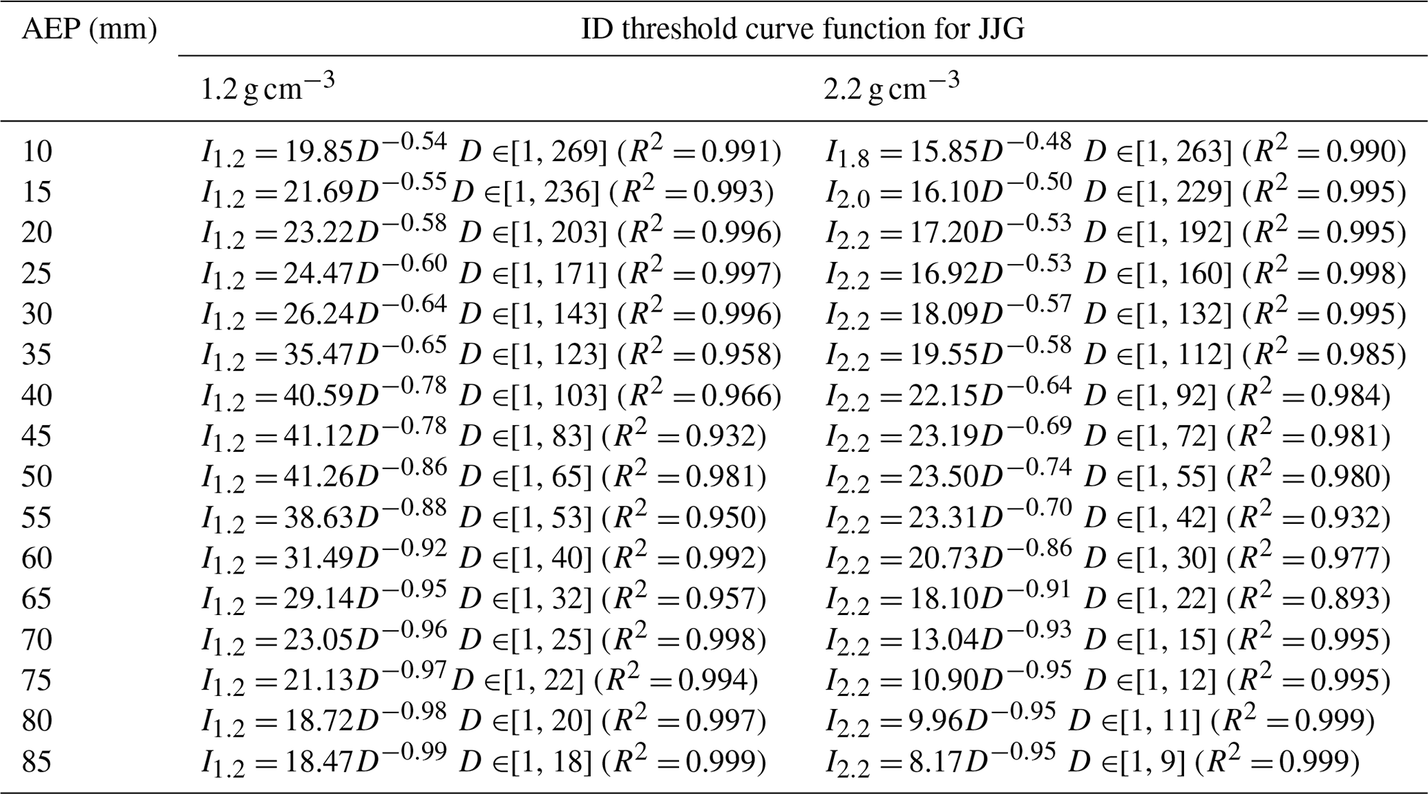
Under the condition of AEP < 10 mm, Dens-ID cannot derive the threshold curve corresponding to even the minimum density value of 1.2 g cm−3, which indicates that the subsequent rainfall can hardly trigger debris flow in JJG. Table 1 also shows that the AEP ranging from 10 to 85 mm can significantly affect the ID threshold curve because the parameters including α and β regularly respond to the change in AEP.
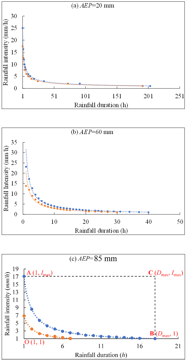
Figure 2ID threshold curves derived by Dens-ID (the blue dotted line corresponds to 1.2 g cm−3, and the orange dotted line corresponds to 2.2 g cm−3).
There are two ID threshold curves in each panel of Fig. 2, which correspond to 1.2 and 2.2 g cm−3, respectively. Because the debris flow density in JJG varies within a certain range from 1.2–2.3 g cm−3, the two ID threshold curves shown in each panel can be regarded as the upper and lower boundary lines for determining the occurrence of debris flow (Zhang et al., 2020). Within the ID coordinate system, the two derived curves together with the I and D axes delineate a closed area shown in Fig. 2c. Any subsequent rainfall represented by the combination of I and D falling into WID may trigger a debris flow. As shown in each panel, the threshold curve can be represented by the power function I=αDβ. The variation intervals of the independent (D) and dependent (I) variables of the power function are [1, Dmax] and [1, Imax], respectively, where Dmax represents the rainfall duration required to trigger debris flow when I= 1 mm h−1, and Imax represents the rainfall intensity required for debris flow formation for D= 1 h. As shown in Fig. 2c, the independent variable D and dependent variable I can delineate a larger rectangular area (AOBC) in the ID plane than WID, which is denoted as RID. The coverage area of RID is much larger than that of WID, indicating that the proportion of rainfall conditions that can trigger debris flows is low. Therefore, even for AEP = 85 mm, the occurrence probability of debris flows remains low. As shown in each panel, each AEP corresponds to a different WID and RID, which provides basic data for the quantitative evaluation of the effect of different AEP conditions on the occurrence probability of debris flows.
4.2 Occurrence probability of debris flow under different AEP conditions
Based on the Monte Carlo method of calculating the definite integral, it is necessary to explore the probability density function of rainfall duration (D) to calculate the occurrence probability of debris flow under different AEP conditions. For the 1094 rainfall events listed in Table S1, we found that the probability distribution of rainfall duration D in JJG can be described by a power function (Fig. 3). As shown in Fig. 3, the number of samples with D < 1 accounted for 37.7 %, 1 < D < 3 for 23.5 %, 3 < D < 5 for 14.7 %, and 5 < D < 10 for 16.9 %; the number of rainfall events with D exceeding 10 h accounted for only 6.7 %.
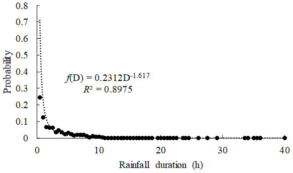
Based on the probability density distribution function , the cumulative probability function cdf(D) can be obtained through integration. In cdf(D), denoted as in Eq. (13), the integration constant C needs to be determined.
The range of 0–40 h is evenly divided into 56 statistical intervals (the second column in Table S2), and each statistical interval is separated by 0.5 h. The proportion of the sample size in each interval among the 1094 samples can be calculated and listed in the second column in Table S2; the cumulative proportion that increases with D is also derived and listed in the third column in Table S2. The data in the first and third columns of Table S2 are substituted into Eq. (13) to calculate C. The results show that C increases with D but gradually stabilizes at approximately 1.04 (the fifth column in Table S2). Therefore, C is set to 1.04.
Based on the process of calculating Pdf under different AEP conditions in Sect. 3.4, the Pdf corresponding to each AEP in Table 1 is obtained, and the function Pdf=f(AEP) for describing their relationship has been fitted using the AEP and Pdf data.
As shown in Eq. (14), the relationship of AEP and Pdf obeys the rule of exponential function as AEP changes from 10 to 85 mm, whereas Pdf=0 when AEP is less than 10 mm. The evolution of Pdf with AEP variation can be divided into two stages (Fig. 4). Two key issues must be stated before discussing the two stages in depth. (1) Based on the calculation results of the Dens-ID model, an upper limit volume of the rainfall-induced solid material supply is derived in JJG, which is the basic condition for determining the scale of debris flow in JJG (Zhang et al., 2020). (2) Based on the principle of water balance, AEP is defined as the rainfall that is preserved in the soil before the triggering rainfall process (Kohler and Linsley, 1951); field observations in JJG show that the AEP is positively correlated with the soil water content (Cui et al., 2007), and the field observations of the Liudaogou catchment in the northern Loess Plateau of China have the same result (Zhu and Shao, 2008). Therefore, the AEP is typically used to estimate soil water content (Crozier, 1986; Chen et al., 2018; Zhao et al., 2019b). The water soil content before the triggering rainfall process can be characterized by AEP (Thomas et al., 2019; Schoener and Stone, 2020).
Stage 1. The probability of debris flow occurrence in JJG is equal to 0 when the AEP is < 10 mm. Dens-ID estimates the solid material volume by simulating rainfall-induced shallow landslides. According to Eq. (4), the key hydrological process that triggers shallow landslides is the continuous increase in soil water content caused by rainfall infiltration. The increase in soil moisture content reduces soil matrix suction and eventually contributes to shallow landslides. The soil water content of the loose soil mass in JJG is low when the AEP < 10 mm (Long et al., 2020), and a long duration of rainfall infiltration is needed to increase the soil water content. However, based on the infiltration border of Dens-ID (Eq. 1), limited by the infiltration capacity of the topsoil in JJG, the portion of precipitation that exceeds the infiltration capacity is be converted into runoff; therefore, when the water content of the soil layer in JJG is low, the surface runoff can be rapidly generated. Therefore, the runoff generation rate can be much higher than the supply rate of solid material in the condition of AEP < 10 mm. In this hydrological scenario, Dens-ID determines that even a soil–water mixture with a density of 1.2 g cm−3 is difficult to generate in JJG; thus, the probability of debris flow is 0.
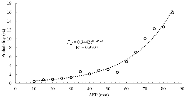
Stage 2. When AEP varies within the interval of 10–85 mm, the subsequent rainfall is capable of triggering debris flow in JJG. Compared to AEP < 10 mm in Stage 1, the soil water content within JJG increased significantly. Therefore, the solid material from shallow landslides can be immediately ready without a long rainfall infiltration duration, and a large water content of topsoil is beneficial to the rapid generation of runoff (Jones et al., 2017; Hirschberg et al., 2021). When there is a sufficient supply of solid material and runoff, the probability of debris flow occurrence in Stage 2 is significantly increased by the increasing AEP. The relationship between Pdf and AEP can be described by an exponential function of Pdf=0.3442e0.0457AEP. The exponential function and its boundary show that the increasing tendency of Pdf is a little sluggish before AEP is equal to 50 mm. The occurrence probability of debris flow in JJG is only 15.88 % even when AEP is equal to 85 mm.
5.1 Correlation analysis of the two curves derived from Dens-ID and observation data
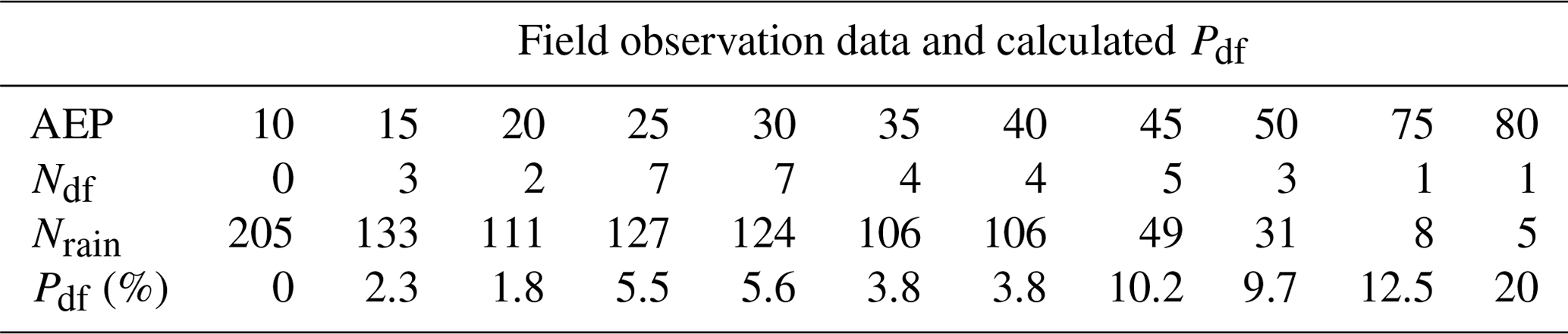
The AEP in Table S1 varied from 0–87.9 mm, and according to this range, we can test the reasonability of the relationship between Pdf and AEP shown in Fig. 4. We introduce how to use the rainfall and debris flow data recorded in Table S1 to calculate Pdf. (1) The original AEP value is rounded to one decimal place, and the rounded AEP values are listed in the eighth column of Table S1, sorted from largest to smallest. (2) The maximum AEPi was set to 85 mm, and [AEPi, AEPi−5] was used as the search window to collect the rainfall events and debris flow events. (3) We count the number of debris flow events Ndf and the number of rainfall events Nrain in each search window and then calculate . Based on the above steps, the collected data and calculated Pdf values are listed in Table 2. As shown in Table 2, a positive correlation between the probability of debris flow occurrence and AEP in JJG was determined. When AEP < 10 mm, a total of 205 rainfall processes were recorded; however, no debris flow events were observed, and the debris flow occurrence probability was 0, which is consistent with the results of Stage 1 derived from Dens-ID.
Based on Pdf and AEP values listed in Table 2, their relationship can be described by the exponential function denoted as Pdf=1.5917e0.031AEP, which is similar to Eq. (14) drawn in Fig. 4. The two curves were nearly parallel. Equation (12) was used to analyze the correlation of the two curves, and r is equal to 0.93, suggesting they have a very high correlation. Therefore, the function of Pdf=f(AEP) derived from Dens-ID, which is used to describe the evolution trend of debris flow occurrence probability with AEP variation, is reasonable.
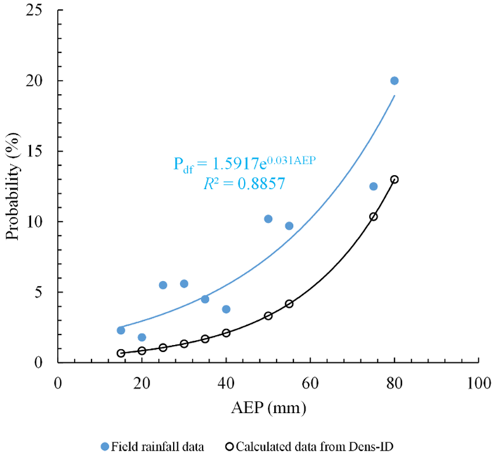
Figure 5Relationship of AEP and Pdf obtained from field observation data and Dens-ID model (the blue line is derived from field observation data, and the black line is derived from Dens-ID).
We can also see from Fig. 5 that although the variation tendencies of the two curves are consistent, a significant bias existed between them. Basically, the probability value derived from the field observation data is larger than that from the Dens-ID model in the condition of a given AEP. As shown in Fig. 5, the blue line fitted through the observation data is above the black line derived from Dens-ID, indicating that Dens-ID underestimated the probability of debris flow occurrence if the observation data were used as the reference. Taking the probability value in the sixth row of Table 2 as a reference, the error of Eq. (14) was calculated using the AEP in Table 2 as input and is listed in Table 3.
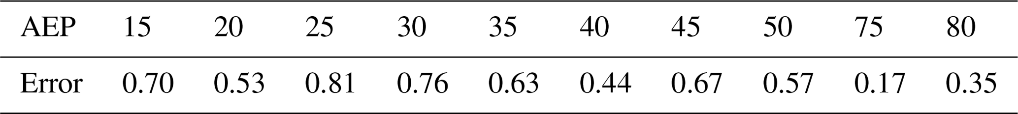
It can be seen that very large bias of Eq. (12) is listed in Table 2. However, we cannot conclude that there is a precision problem in the calculation results of the Dens-ID. This is for two reasons. (1) Although 1094 rainfall processes and 37 debris flow events are the field observation data, there are many uncertain factors in Eq. (7) for calculating AEP using these rainfall data (Kim et al., 2021), such as the subjectivity existing inK and n of Eq. (7), which introduce uncertainty into the calculated AEP. In this case, if the data in Table S1 are used as the real value for evaluating the precision of Dens-ID, the error evaluation result may be unfair to Dens-ID. In this case, it is unfair to evaluate the Dens-ID error using the calculated AEP in Table S1 as the true value. However, this uncertainty can show consistent directional deviations because of the fixed values of K and n in Eq. (7); therefore, the uncertainty has no effect on the correlation analysis. (2) To establish the functional relationship between Pdf and AEP, many rainfall scenarios were simulated using the Dens-ID model. Dens-ID simulated 3376, 3182, 2677, and 2677 rainfall processes with AEP = 20, 40, 45, and 50 mm, respectively. The total number of simulated rainfall processes was significantly larger than that of the 1094 observed rainfall events. The collected 1094 rainfall events still cannot fully reflect all rainfall conditions in nature; that is, the number of observed rainfall data, 1094, is still inadequate when used as the denominator for calculating the probability of debris flow occurrence in JJG. Therefore, the Pdf calculated using the field observation data may be generally higher than that calculated using Dens-ID. With the accumulation of rainfall observation data of JJG, it is believed that the Pdf derived from field observation data will gradually decrease until it is close to the calculated value of the Dens-ID model. (3) Dens-ID cannot fully and accurately describe the formation process of the debris flow in JJG because of the simplification in theory and boundaries. Dens-ID is also affected by the accuracy of the input parameters (Zhang et al., 2020), which may eventually lead to deviations between the simulation results and field observations.
5.2 Potential application and limitation
Deriving a quantified functional relationship of Pdf and AEP would be more conducive to examining the correspondence between these two parameters. Using a mathematical physics method, the function of Pdf=f(AEP) was firstly derived, which can help us to learn more from the derived Pdf=f(AEP).
Firstly, AEP is indeed an important factor affecting debris flow. Generally, there is the following consensus in the field of debris flow: the greater the AEP, the higher the probability (Pdf) of subsequent rainfall triggering the debris flow (De Vita et al., 2000; Bel et al., 2017). However, this fuzzy qualitative description cannot explain the influence degree of AEP on the probability of debris flow induced by subsequent rainfall. It can be seen from Pdf=f(AEP) that there are two key value nodes of AEP affecting Pdf:
-
The case of AEP < 10 mm indicates that any subsequent rainfall cannot trigger debris flow in JJG. Because the supply rate of solid material is much lower than the runoff generation rate during subsequent rainfall in JJG, the water–soil mixture within tends to be a hyperconcentrated flow rather than a debris flow (Long et al., 2020).
-
The case of 10 mm ≤ AEP ≤ 50 mm means that the soil water content increases significantly compared to AEP < 10 mm, but a necessary infiltration time to increase it to the critical state for triggering shallow landslides is still required. Therefore, limited by the supply rate of the solid material, the increasing rate of Pdf is sluggish. The case of 50 mm < AEP ≤ 85 mm shows that the soil water content is relatively larger, the solid material from shallow landslides can be immediately ready without a long rainfall infiltration duration, and a large soil water content of topsoil is beneficial to the rapid generation of runoff (Jones et al., 2017; Hirschberg et al., 2021). When there is a sufficient supply of provenance and runoff, the probability of debris flow occurrence in this subprocess is significantly enhanced by the increasing AEP.
Secondly, rainfall-induced debris flow is a small-probability event compared with the rainfall frequency in nature. JJG is well known due to its high-frequency debris flow event. However, the formation probability of debris flow in JJG induced by subsequent rainfall is only 15.88 %, even when the AEP reaches 85 mm. Therefore, debris flow induced by rainfall in JJG is a small-probability event compared with the rainfall frequency. The figure of 15.88 % means that the efficiency of rain-induced debris flow is extremely low, which also indicates that the formation of debris flow is an extremely complex physical process, in which rainfall is only one of the motivating factors, and there are other more important internal factors affecting the formation of debris flow, such as topography, source recharge, and fluid characteristics of debris flow (Zhang et al., 2020). Thirdly, in practical application, when the AEP in JJG is calculated according to Eq. (7), the derived exponential function can help us to assess the probability of debris flow in JJG triggered by subsequent rainfall, according to which debris flow warning information can be issued in advance to provide technical support for disaster prevention and reduction.
Our study also has its own limitations and needs to be listed for providing directions for subsequent investigation. (1) Long-term observation data should be used to deduce the functions of Pdf=f(AEP); however, the number of debris flow gullies with long-term observational data worldwide is less than 10 (Hürlimann et al., 2019). Accordingly, the function of Pdf=f(AEP) cannot yet be derived in other debris flow gullies. (2) The Dens-ID model assumes that the solid material mainly comes from shallow landslides. However, the formation mechanism and solid source supply mode of runoff-induced debris flow are different. Therefore, the functional of Pdf=f(AEP) for runoff-induced debris flow still needs to be studied with the help of other physical models. (3) The calculation result of Pdf=f(AEP) derived from Dens-ID model has a large bias from the observation data; the authors think that the main reason is insufficient field observation data, especially inadequate rainfall data. Basically, even for high-frequency debris flow gullies like JJG, the success rate of debris flow induced by rainfall is still very low. A continuous increase in rainfall and debris flow observation data will make the growth rate of Nrain in Table 2 much higher than that of Ndf. Therefore, with the accumulation of rainfall observation data of JJG, it is believed that the Pdf derived from field observation data will gradually decrease until it is close to the calculated result of Dens-ID model. Therefore, the authors will continue to collect field observation data of JJG in the later period and constantly verify the accuracy of Eq. (14) derived from Dens-ID.
The Dens-ID model and Monte Carlo integral equation is used to derive function of Pdf=f(AEP). The functional relationship is verified using a large number of field observation data from JJG. The following conclusions are drawn.
The positive relationship between Pdf and AEP is now described by a clear mathematical equation in this study. The range of AEP that can affect debris flow formation is verified within 10–85 mm. Based on the simulation results, the probability of debris flow occurrence in JJG is 0 in conditions where AEP < 10 mm, and the relationship between Pdf and AEP can be described by an exponential function when 10 mm ≤ AEP ≤ 85 mm. The plausibility of the first two evolution stages of the Pdf–AEP piecewise function is effectively confirmed by the field observation data because the Pdf–AEP relationship obtained from field observation data is highly correlated with the simulation results of Dens-ID. However, the reasonability of the last two stages of the Pdf–AEP piecewise function cannot be tested because of the lack of field observation data, and the errors of the Pdf–AEP piecewise function cannot be verified because of the uncertainty of the AEP derived from the observation rainfall data.
This study mathematically confirms that the greater the AEP, the higher the probability of subsequent rainfall triggering debris flow and quantifies this qualitative conclusion using piecewise functions. This can effectively reveal the essential relationship between the two natural events of rainfall and debris flow, quantitatively describe the impact of different AEP conditions on the probability of debris flow occurrence, and provide key technical support for the early warning of debris flows.
Some or all data, models, or code generated or used during the study are available from the corresponding author by request. The code can be downloaded through https://pan.baidu.com/disk/main?from=homeFlow#/index?category=all&path=%2F (Zhang, 2024). The key underlying research data are listed in Tables S1–S3 in the Supplement.
The supplement related to this article is available online at: https://doi.org/10.5194/hess-28-2343-2024-supplement.
SZ, XL, HY, JM, and DL conceptualized the work; developed the methodology; and carried out the data curation, formal analysis, validation, and writing of the original draft. FW and KH reviewed the initial manuscript.
The contact author has declared that none of the authors has any competing interests.
Publisher's note: Copernicus Publications remains neutral with regard to jurisdictional claims made in the text, published maps, institutional affiliations, or any other geographical representation in this paper. While Copernicus Publications makes every effort to include appropriate place names, the final responsibility lies with the authors.
This research has been supported by the National Key Research and Development Program of China (grant no. 2023YFC3007205), the West Light Foundation of the Chinese Academy of Science, the National Natural Science Foundation of China (grant nos. 42271013 and 42001100), and a project of the Department of Science and Technology of Sichuan Province (grant no. 2023ZHCG0012).
This paper was edited by Lelys Bravo de Guenni and reviewed by two anonymous referees.
Abraham, M. T., Satyam, N., Pradhan, B., and Alamri, A. M.: Forecasting of landslides using rainfall severity and soil wetness: A probabilistic approach for Darjeeling Himalayas, Water (Switzerland), 12, 1–19, 2020.
Abraham, M. T., Satyan, N., Rosi, A., Pradhan, B., and Segoni, S.: Usage of antecedent soil moisture for improving the performance of rainfall thresholds for landslide early warning, Catena, 200, 105147, https://doi.org/10.1016/j.catena.2021.105147, 2021.
Adams, B., Fraser, H., Howard, C., and Hanafy, M.: Meteorological data analysis for drainage system design, J. Environ. Eng., 112, 827–848, https://doi.org/10.1061/(ASCE)0733-9372(1986)112:5(827), 1986.
Albert, G. E.: A general theory of stochastic estimates of the Neumann series for solution of certain Fredholm integral equations and related series, in: Symposium of Monte Carlo Methods, edited by: Meyer, M. A., Wiley, New York, https://www.osti.gov/servlets/purl/4427633 (last access: 29 May 2024), 1956.
Bel, C., Liébault, F., Navratil O., Eckert N., Bellot H., Fontaine, F., and Laigle, D.: Rainfall control of debris-flow triggering in the Réal Torrent, Southern French Prealphs, 291, 17–32, 2017.
Bennett, G. L., Molnar, P., Mcardell, B. W., and Burlando, P.: A probabilistic sediment cascade model of sediment transfer in the Illgraben, Water Resour. Res., 50, 1225–1244, 2014.
Bernard, M. and Gregoretti, C.: The use of rain gauge measurements and radar data for the model-based prediction of runoff-generated debris flow occurrence in early warning systems, Water Resour. Res., 57, e2020WR027893, https://doi.org/10.1029/2020WR027893, 2021.
Berti, M. and Simoni, A.: Experimental evidences and numerical modelling of debris flow initiated by channel runoff, Landslides, 3, 171–182, 2005.
Calvo, B. and Savi, F.: A real-world application of Monte Carlo procedure for debris flow risk assessment, Comput. Geosci., 35, 967–977, 2009.
Castillo, V. M., Gómez-Plaza, A., and Martínez-Mena, M.: The role of antecedent soil water content in the runoff response of semiarid catchments: a simulation approach, J. Hydrol., 284, 114–130, 2003.
Chen, C. W., Oguchi, T., Chen, H., and Lin, G. W.: Estimation of the antecedent rainfall period for mass movements in Taiwan, Environ. Earth Sci., 77, 184, https://doi.org/10.1007/s12665-018-7377-7, 2018.
Chen, C. W., Saito, H., and Oguchi, T.: Analyzing rainfall-induced mass movements in Taiwan using the soil water index, Landslides, 14, 1031–1041, 2017.
Coe, J. A., Kinner, D. A., and Godt, J. W.: Initiation conditions for debris flows generated by runoff at Chalk Cliffs, central Colorado, Geomorphology, 3, 270–297, 2008.
Crozier, M. J.: Landslides: causes, consequences & environment, Croom Helm, London, p. 25, https://www.cabidigitallibrary.org/doi/full/10.5555/19871915008 (last access: 29 May 2024), 1986.
Cui, P., Zhu, Y. Y., Chen, J., Han, Y. S., and Liu, H. J.: Relationships between antecedent rainfall and debris flows in Jiangjia Ravine, China, in: Debris-Flow Hazards Mitigation: Mechanics, Prediction, and Assessment, edited by: Chen, C. and Major, J., Millpress, Netherlands, 3–10, https://webofscience.clarivate.cn/wos/alldb/summary/c8412688-7797-4f83-adb1-214f3747ca8f-ed3972c7/relevance/1 (last access: 30 May 2024), 2007.
De Paola, F., De Risi, R., Di Crescenzo, G., Giugni, M., Santo, A., and Speranza, G.: Probabilistic Assessment of Debris Flow Peak Discharge by Monte Carlo Simulation, Journal of Risk and Uncertainty in Engineering Systems, Part A: Civil Engineering, 3, A4015002, https://doi.org/10.1061/AJRUA6.0000855, 2017.
De Vita, P.: Fenomeni d'instabilita` delle coperture piroclastiche dei Monti Lattari, di Sarno e di Salerno (Campania) ed analisi degli eventi pluviometrici determinanti, Quad. Geol. Appl., 7, 213–239, 2000.
Donovan, I. P. and Santi, P. M.: A probabilistic approach to post-wildfire debris-flow volume modeling, Landslides, 14, 1345–1360, 2017.
Fiorillo, F. and Wilson, R. C.: Rainfall induced debris flows in pyroclastic deposits, Campania (southern Italy), Eng. Geol., 75, 263–289, 2004.
Gabet, E. J. and Mudd, S. M.: The mobilization of debris flows from shallow landslides, Geomorphology, 1, 207–218, 2006.
Han, Z., Chen, G. Q., Li, Y. G., and He, Y.: Assessing entrainment of bed material in a debris-flow event: a theoretical approach incorporating Monte Carlo method: Assessing Entrainment of Bed Material by Debris Flow, Earth Surf. Proc. Land., 40, 1877–1890, 2015.
Hirschberg, J., Badoux, A., McArdell, B. W., Leonarduzzi, E., and Molnar, P.: Evaluating methods for debris-flow prediction based on rainfall in an Alpine catchment, Nat. Hazards Earth Syst. Sci., 21, 2773–2789, https://doi.org/10.5194/nhess-21-2773-2021, 2021.
Hong, M., Kim, J., and Jeong, S.: Rainfall intensity-duration thresholds for landslide prediction in South Korea by considering the effects of antecedent rainfall, Landslides, 15, 523–534, 2018.
Hu, W., Xu, Q., Wang, G. H., van Asch, T. W. J., and Hicher, P. Y.: Sensitivity of the initiation of debris flow to initial soil moisture, Landslides, 12, 1139–1145, 2015.
Huang, C. H.: Critical rainfall for typhoon-induced debris flows in the Western Foothills, Taiwan, Geomorphology, 185, 87–95, 2013.
Hürlimann, M., Coviello, V., Bel, C., Guo, X. J., Berti, M., Graf, C., Hübl, J., Miyata, S., Smith, J. B., and Yin, H. Y.: Debris-flow monitoring and warning, Review and examples, Earth-Sci. Rev., 199, 102981, https://doi.org/10.1016/j.earscirev.2019.102981, 2019.
Iverson, R. M., Reid, M. E., and LaHusen, R. G.: Debris Flow Mobilization from Landslides, Annu. Rev. Earth Pl. Sc., 25, 85–138, 1997.
Jones, R., Thomas, R. E., Peakall, J., and Manville, V.: Rainfall-runoff properties of tephra: Simulated effects of grain-size and antecedent rainfall, Geomorphology, 282, 39–51, 2017.
Kim, S. W., Chun, K. W., Kim, M., Catani, F., Choi, B., and Seo, J.: Effect of antecedent rainfall conditions and their variations on shallow landslide-triggering rainfall thresholds in South Korea, Landslides, 18, 569–582, 2021.
Kohler, M. A. and Linsley, R. K.: Predicting the runoff from Storm Rainfall, US Department of Commerce, Weather Bureau, Washington, D.C., https://www.nrc.gov/docs/ML0819/ML081900279.pdf (last access: 29 May 2024), 1951.
Le Bissonnais, Y., Renaux, B., and Delouche, H.: Interactions between soil properties and moisture content in crust formation, runoff and interrill erosion from tilled loess soils, Catena, 25, 33–46, 1995.
Li, L., Zhang, S. X., Li, S. H., Qiang, Y., Zheng, Z., and Zhao, D. S.: Debris Flow Risk Assessment Method Based on Combination Weight of Probability Analysis, Advances in Civil Engineering, 2021, 1–12, https://doi.org/10.1155/2021/6640614, 2021.
Liu, D. L., Zhang, S. J., Yang, H. J., Zhao, L. Q., Jiang, Y. H., Tang, D., and Leng, X. P.: Application and analysis of debris-flow early warning system in Wenchuan earthquake-affected area, Nat. Hazards Earth Syst. Sci., 16, 483–496, https://doi.org/10.5194/nhess-16-483-2016, 2016.
Liu, X. L., Wang, F., Nawnit, K., Lv, X. F., and Wang, S. J.: Experimental study on debris flow initiation, B. Eng. Geol. Environ., 79, 1565–1580, 2020.
Long, K., Zhang, S. J., Wei, F. Q., Hu, K. H., Zhang, Q., and Luo, Y.: A hydrology-process based method for correlating debris flow density to rainfall parameter and its application on debris flow prediction, J. Hydrol., 589, 125124, https://doi.org/10.1016/j.jhydrol.2020.125124, 2020.
Luk, S. H.: Effect of antecedent soil moisture content on rainwash erosion, Catena, 12, 129–139, 1985.
Marra, F., Destro, E., Nikolopoulos, E. I., Zoccatelli, D., Creutin, J. D., Guzzetti, F., and Borga, M.: Impact of rainfall spatial aggregation on the identification of debris flow occurrence thresholds, Hydrol. Earth Syst. Sci., 21, 4525–4532, https://doi.org/10.5194/hess-21-4525-2017, 2017.
Papa, M. N., Medina, V., Ciervo, F., and Bateman, A.: Derivation of critical rainfall thresholds for shallow landslides as a tool for debris flow early warning systems, Hydrol. Earth Syst. Sci., 17, 4095–4107, https://doi.org/10.5194/hess-17-4095-2013, 2013.
Peres, D. J. and Cancelliere, A.: Derivation and evaluation of landslide-triggering thresholds by a Monte Carlo approach, Hydrol. Earth Syst. Sci., 18, 4913–4931, https://doi.org/10.5194/hess-18-4913-2014, 2014.
Peres, D. J. and Cancelliere, A.: Modeling impacts of climate change on return period of landslide triggering, J. Hydrol., 567, 420–434, 2018.
Richards, L. A.: Capillary condition of liquids in porous mediums, Physics, 1, 318–333, 1931.
Schoener, G. and Stone, M. C.: Monitoring soil moisture at the catchment scale-A novel approach combing antecedent precipitation index and rader-derived rainfall data, J. Hydrol., 589, 125155, https://doi.org/10.1016/j.jhydrol.2020.125155, 2020.
Segoni, S., Rosi, A., Lagomarsino, D., Fanti, R., and Casagli, N.: Brief communication: Using averaged soil moisture estimates to improve the performances of a regional-scale landslide early warning system, Nat. Hazards Earth Syst. Sci., 18, 807–812, https://doi.org/10.5194/nhess-18-807-2018, 2018.
Senthilkumar, V., Chandrasekaran, S. S., and Maji, V. B.: Geotechnical characterization and analysis of rainfall-induced 2009 landslide at Marappalam area of Nilgiris district, Tamil Nadu state, India, Landslides, 14, 1803–1814, 2017.
Tang, H., Mcguire, L. A., Kean, J. W., and Smith, J. B.: The impact of sediment supply on the initiation and magnitude of runoff-generated debris flows, Geophys. Res. Lett., 47, e2020GL087643, https://doi.org/10.1029/2020GL087643, 2020.
Thomas, M. A., Collins, B. D., and Mirus, B. B.: Assessing the feasibility of satellite-based thresholds for hydrologically driven landsliding, Water Resour. Res., 55, 9006–9023, 2019.
Tisdall, A.: Antecedent soil moisture and its relation to infiltration, Aust. J. Agr. Res., 2, 342–348, 1951.
Van Genuchten, M.: A closed form equation for predicting the hydraulic conductivity of unsaturated soils, Soil Sci. Soc. Am. J., 44, 892–898, 1980.
Wei, F. Q., Hu, K. H., Zhang, J., Jiang, Y. H., and Chen, J.: Determination of effective antecedent rainfall for debris flow forecast based on soil moisture content observation in Jiangjia Gully, China, in: Monitoring, Simulation, Prevention and Remediation of dense debris flows II, edited by: DeWrachien, D., Brebbia, C. A., and Lenzi, M. A., WIT Transactions on Engineering Sciences, England, 13–22, https://doi.org/10.2495/DEB080021, 2008.
Yan, Z. Z. and Hong, Z. M.: Using the Monte Carlo method to solve integral equations using a modified control variate, Appl. Math. Comput., 242, 764–777, 2014.
Yang, H. J., Zhang, S. J., Hu, K. H., Wei, F. Q., Wang, K., and Liu, S.: Field observation of debris flow activities in the initiation area of Jiangjia Gully, Yunnan Province, China, J. Mt. Sci., 19, 1602–1617, 2022.
Zeng, Q. L., Yue, Z. Q., Yang, Z. F., and Zhang, X. J.: A case study of long-term field performance of check-dams in mitigation of soil erosion in Jiangjia stream, China, Environ. Geol., 58, 897–911, 2009.
Zhang, S.: JJG, DENS-ID [code], https://pan.baidu.com/disk/main?from=homeFlow#/index?category=all&path=%2F, last access: 28 May 2024.
Zhang, S. J., Xu, C. X., Wei, F. Q., Hu, K. H., Xu, H., Zhao, L. Q., and Zhang, G. P.: A physics-based model to derive rainfall intensity-duration threshold for debris flow, Geomorphology, 351, 106930, https://doi.org/10.1016/j.geomorph.2019.106930, 2020.
Zhang, S. J., Yang, H. J., Wei, F. Q., Jiang, Y. H., and Liu, D. L.: A model of debris flow forecast based on the water-soil coupling mechanism, J. Mt. Sci., 25, 757–763, 2014.
Zhang, S. J., Xia, M. Y., Li, L., Yang, H. J., Liu, D. L., and Wei, F. Q.: Quantify the effect of antecedent effective precipitation on rainfall intensity-duration threshold of debris flow, Landslides, 20, 1719–1730, 2023.
Zhao, B. R., Dai, Q., Han, D. W., Dai, H. C., Mao, J. Q., and Zhuo, L.: Probabilistic thresholds for landslides warning by integrating soil moisture conditions with rainfall thresholds, J. Hydrol., 574, 276–287, 2019a.
Zhao, B. R., Dai, Q., Han, D., Dai, H., Mao, J., Zhuo, L., and Rong, G.: Estimation of soil moisture using modified antecedent precipitation index with application in landslide predictions, Landslides, 16, 2381–2393, 2019b.
Zhu, Y. J. and Shao, M. G.: Variability and pattern of surface moisture on a small-scale hillslope in Liudaogou catchment on the northern Loess Plateau of China, Geoderma, 147, 185–191, 2008.
Zhuang, J. Q., Cui, P., Wang, G. H., Chen, X. Q., Iqbal, J., and Guo, X. J.: Rainfall thresholds for the occurrence of debris flows in Jiangjia Gully, Yunnan Province, China, Eng. Geol., 195, 335–346, 2015.