Accounting for hydroclimatic properties in flood frequency analysis procedures

Flood hazard is typically evaluated by computing extreme flood probabilities from a flood frequency distribution following nationally defined procedures in which observed peak flow series are fit to a parametric probability distribution. These procedures, also known as flood frequency analysis, typically recommend only one probability distribution family for all watersheds within a country or region. However, large uncertainties associated with extreme flood probability estimates (>50-year flood or Q₅₀) can be further biased when fit to an inappropriate distribution model because of differences in the tails between distribution families. Here, we demonstrate that hydroclimatic parameters can aid in the selection of a parametric flood frequency distribution. We use L-moment diagrams to visually show the fit of gaged annual maxima series across the United States, grouped by their Köppen climate classification and the precipitation intensities of the basin, to a general extreme value (GEV), log normal 3 (LN3), and Pearson 3 (P3) distribution. Our results show that in real space basic hydroclimatic properties of a basin exert a significant influence on the statistical distribution of the annual maxima. The best-fitted family distribution shifts from a GEV towards an LN3 distribution across a gradient from colder and wetter climates (Köppen group D, continental climates) towards more arid climates (Köppen group B, dry climates). Due to the diversity of hydrologic processes and flood-generating mechanisms among watersheds within large countries like the United States, we recommend that the selection of distribution model be guided by the hydroclimatic properties of the basin rather than relying on a single national distribution model.

1 Introduction

Around the world, communities depend on rivers for vital resources, yet riverine floods present a significant hazard for people and infrastructure along interior waterways (Mallakpour and Villarini, 2015; Peterson et al., 2013). To mitigate risks and develop safe emergency plans, water managers depend on reliable methods to compute extreme flood probabilities. Typically these methods use the probability distribution of annual maxima discharge, also known as the flood frequency distribution, from which one can compute extreme flood probabilities (e.g., the 100-year flood (Q₁₀₀), a flood with a 1 % chance of occurrence in a given year) (Hamed and Ramachandro Rao, 2000; Kidson and Richards, 2005; Cassalho et al., 2019). To construct flood frequency distributions, national flood frequency procedures around the world fit observed annual stream maxima to a parametric probability distribution model (Castellarin et al., 2012; Madsen et al., 2014). These approaches involve and are affected by the a priori assumption regarding which parametric statistical model best captures the empirical distribution of flood magnitudes (Kidson and Richards, 2005). Standard national procedures often prescribe just one probabilistic distribution model; for example, the United States Bulletin 17C recommends the log-Pearson 3 (LP3) distribution family (England et al., 2019), while in the United Kingdom, the Flood Estimation Handbook (FEH) recommends the use of the generalized logistic distribution (GLO) (Robson and Reed, 1999). Although these recommendations provide a consistent framework for flood frequency analyses (Barth et al., 2019), they can also result in biased estimates of infrequent flood probabilities when applied over large hydro-climatically diverse regions (Klemes, 1993; Merz and Blöschl, 2003, 2008), due to the inherent differences in the distribution shape and tail thickness of different parametric models. These differences can amplify the existing large uncertainties for extreme flood probability estimates, such as the 100- or 500-year floods.

Watershed morphology, land use management, and climatology affect flood frequency properties such as the mean, variance, and tails or, respectively, the location, scale, and shape parameters of the probabilistic distribution. For example, large watersheds have the capacity to absorb heavy precipitation events better than small watersheds (Iacobellis et al., 2002; Salinas et al., 2014b), meaning that peak flow in smaller watersheds is disproportionally affected by an extreme precipitation event and that they observe higher peak flow variances (Iacobellis et al., 2002; Salinas et al., 2014a). Other studies have noted more complex relationships, where the coefficient of variation (CV) of flood frequency distributions decreases with watershed area for small watersheds but increases with area for large watersheds (Blöschl and Sivapalan, 1997; Smith, 1992). Urbanization leads to a reduction in soil permeability and an increase in precipitation-induced surface runoff (Hall et al., 2014; Hodgkins et al., 2019), which results in more local flash floods that are associated with thick-tailed flood frequency distributions (Merz and Blöschl, 2003; Zhang et al., 2018) – although this effect is strongest for regular floods and diminishes for increasing exceedance probabilities (Over et al., 2016). Relatedly, population growth (a proxy for urbanization) and river engineering (e.g., channel straightening) can increase mean annual peak flows (Villarini et al., 2009; Munoz et al., 2018), whereas dam reservoirs have reduced the median annual flood by up to 25 % in 55 % of the large US rivers (Fitzhugh and Vogel, 2011).

Local flood-generating mechanisms, particularly the type, duration, and intensity of local precipitation events, affect all aspects of the flood frequency distribution (Hall et al., 2014; Merz and Blöschl, 2003). In watersheds where precipitation occurs predominantly as rain as opposed to snow, flood frequency distributions exhibit higher variance (Merz and Blöschl, 2003; Gaál et al., 2015). Similarly, watersheds where total annual precipitation only falls in a few intense events also have flood distributions with high CV (Blöschl and Sivapalan, 1997; Pitlick, 1994), whereas watersheds with high total annual precipitation observe flood distributions with lower CV (Salinas et al., 2014b). Merz and Blöschl (2003) summarized several of these findings in their typology of regional flood-generating mechanisms. Antecedent soil moisture adds another level of complexity to the relationship between precipitation and flood frequency distribution shape, as synchronicity between precipitation and antecedent soil moisture levels is likely to thicken the flood frequency distribution tails through surface runoff levels (Ivancic and Shaw, 2015).

The patterns between local watershed characteristics and flood frequency distribution properties form a potential tool for improving extreme flood probability estimates in hydrologically diverse regions. One method is to select a parametric distribution based on the value of an environmental parameter of the watershed, for example a precipitation statistic or a drainage area. Salinas et al. (2014b) demonstrate that European rivers with different drainage areas and total annual precipitation fit differently to multiple three-and-two-parameter distribution families. However, as described above, the relation between drainage area and flood frequency shape is complex, and annual maximum rainfall does not necessarily reflect different precipitation regimes. There are relatively few studies that relate flood frequency distributions to aggregated climate classifications such as the Köppen climate regions (Kottek et al., 2006; Peel et al., 2007). In one such study, Metzger et al. (2020) demonstrate that flood frequency distributions in arid and semi-arid regions give larger ratios of 10- to 100-year floods compared to Mediterranean climates; a similar relation was found when arid regions are compared to humid regions (Zaman et al., 2012). These findings provide strong support for the hypothesis that the hydroclimatic properties of a basin – particularly aggregate hydroclimatic classifications like the Köppen system – influence the tail thickness of flood frequency distributions and thus exert considerable influence on the probabilities of the most extreme flood events.

Here we build on the previous work by Salinas et al. (2014a, b) by examining the fit of annual maxima streamflow data from across the United States to several three-parameter distributions via L-moment diagrams. We perform a similar experiment but group annual maxima gage records based on two aggregated hydroclimatic variables instead of one-dimensional variables: (1) the Köppen climate region (Kottek et al., 2006) and (2) watershed precipitation intensity, which is a combination of the maximum daily precipitation and the total annual precipitation. We chose the Köppen climate classification because it includes several of the above-mentioned variables that affect peak flow distributions (temperature, precipitation, vegetation, soil properties) and precipitation intensity because it represents aspects of flood-generating precipitation regimes (Hayden, 1988). By grouping gage discharge records based on the hydroclimatic properties of their basin, we assess whether these variables can guide a priori parametric distribution model selection. Our results demonstrate that peak flow records from different Köppen climate regions and precipitation intensity groups tend to fit specific distribution families. These findings imply that the hydroclimate properties of a watershed can be used to guide the selection of a distribution family in flood frequency analysis.

2 Hydroclimatic data and methodology for the L-moment diagrams

2.1 Data

We chose the United States for our study because it spans all five main Köppen climate groups (Peel et al., 2007) and has watersheds that are influenced by a diverse set of synoptic weather systems (Hirschboeck, 1988).

Yet, despite this hydroclimatic diversity, the LP3 distribution is recommended for all flood frequency analyses in the United States in Bulletin 17C (England et al., 2019). To determine the flood frequency distribution shape of different United States rivers, we constructed a dataset containing 1538 annual maxima discharge records (Fig. 1a). This dataset is a selection of the larger USGS surface water database which contains observational data from a network of gages across the United States (USGS, 2020). To generate our dataset, we first selected all records longer than 30 years. Next, we picked the longest continuous record for each available USGS hydrologic unit to avoid biasing the distribution selection towards more heavily gaged rivers. We also included records from Alaska and Hawaii to encompass additional hydroclimatic diversity. The annual maxima records in the final dataset have an average length of 78 years and a range from 30 to 118 years (Fig. 1b). We also performed a preliminary analyses with a dataset from which records that have been affected by regulation or diversion (USGS qualification code 5 and 6) were omitted; however, this did not yield meaningfully different results (Fig. S1–S3 in the Supplement). As our aim is to find a distribution family that can support a broad range of impacts we decided to also include regulated records.

To classify the gage records in different hydroclimatic groups, each annual maxima record was assigned a Köppen climate classification (Peel et al., 2007; Kottek et al., 2006) and a long-term (1981–2010) daily mean precipitation record from the Climate Prediction Center (CPC) precipitation dataset based on proximity to the centroid of the watershed (Falcone, 2011; Chen et al., 2008). First, annual maxima records were categorized by their main Köppen climate group: arid (B), temperate (C), or continental (D) – other climate groups did not have enough representation among the gages compared to the other climate groups (six for tropical and one for polar – all located in Hawaii or Alaska) (Kottek et al., 2006). Of the 1538 annual maxima, 204 are in an arid climate (Köppen group B), 549 are located in temperate climates (Köppen group C), and 778 are located in continental climates (Köppen group D). Next, we categorized annual maximum records by their watershed's hydroclimatic intensity, defined here as the percentage contribution of the maximum daily precipitation level to the total annual precipitation (P_SC) in the CPC record (Chen et al., 2008). Gages close to high P_SC values thus experience most precipitation during high-intensity events, whereas gages with low P_SC values experience precipitation more evenly throughout the year. We also assessed other precipitation metrics (e.g. annual maximum daily precipitation and the 95th percentile of the daily precipitation level distribution), but these metrics were not as meaningfully associated with flood distributions as P_SC, which is similar to precipitation metrics known to influence flood frequency distribution shape (Metzger et al., 2020; Pitlick, 1994). Each annual maxima record was assigned to one of three groups: the lowest 20 % P_SC values containing 308 records (i.e., precipitation spread more evenly throughout the year), the highest 20 % P_SC values containing 308 records (i.e., a significant proportion of annual precipitation falls in one storm), and all intermediate values encompassing the remaining 922 records. The 20th and 80th percentiles were chosen because they preserve a meaningful difference between the two groups while maintaining large sample sizes.

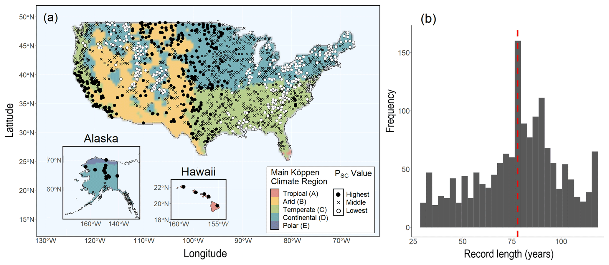
Figure 1 (a) Locations of hydrologic annual maxima records from instrumental river gages used in this study grouped by the percentage of the maximum annual daily precipitation level by the total annual precipitation level (P_SC) and plotted atop their Köppen climate region. (b) Histogram of discharge record length in years; the red line indicates the mean value, 78 years.

2.2 L-moment diagrams

We use L-moment diagrams to measure the fit of annual maxima records to several parametric distribution families. L-moment diagrams are a graphical tool used to assess the goodness-of-fit of multiple annual maxima records to a series of probabilistic models and guide the selection of a regional flood frequency distribution family (Peel et al., 2001; Vogel and Fennessey, 1993). The L-moments of a hydrologic record are the linear combinations of its order statistics and, like regular moments (i.e. the mean, standard deviation, and skewness), describe the shape of a sample distribution. L-moments are often preferred over conventional product moments because they are more robust for small sample sizes (Hosking, 1990; Wang, 1990). When fitting data to three-parameter distributions, an L-moment diagram is constructed by plotting the L-moment ratios of skewness (L-skew; t3), dividing the third L-moment by the second L-moment against the L-moment ratio of kurtosis (L-kurtosis; t4) the fourth L-moment divided by the second L-moment (Hosking and Wallis, 1997). Any three-parameter distribution can be plotted as a line in the L-moment diagram from their mathematical formulation of the ratio between L-skew and L-kurtosis (Table 1). The distance between the L-skew and L-kurtosis of a sample and the line describing a particular three-parameter distribution represents the likelihood of the record deriving from that distribution – the closer the sample to the line, the better the fit (Hosking and Wallis, 1997). A detailed description of L-moments and how to compute them is given by Hosking and Wallis (1997).

Table 1 Overview of the distributions used in this study including their probability density function and L-moments (ratios). Mathematical formulations of the probability density functions and L-moments as described by Hosking and Wallis (1997).

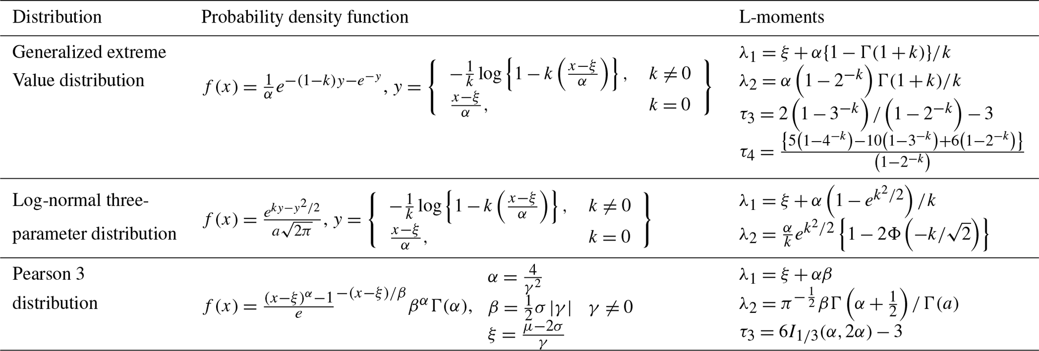
Note: in the probability density functions, ξ, a, and k are the location, scale, and shape parameters, respectively. The symbols λ₁, λ₂, τ₃, and τ₄ respectively stand for the first four L-moments. An approximation of τ₃ and τ₄ for the LN3 and P3 distribution is discussed in detail in Hosking and Wallis (1997).

The L-moments for all annual maxima record in our dataset are compared to a general extreme value (GEV), log normal 3 (LN3), and Pearson 3 (P3) distribution. These three-parameter distributions are commonly used in hydrologic sciences (Salinas et al., 2014b) and are known to fit extreme flood values in the United States well (Vogel et al., 1993; Vogel and Wilson, 1996). Additionally, we plotted log-transformed discharge records in an L-moment diagram to fit them to a LP3 distribution. L-moment diagrams are constructed for all records in the dataset, and each selection of record is based on their Köppen climate classification and P_SC value.

Prior work demonstrated that selecting one distribution that provides the best fit to annual maxima is difficult over a large hydrologically heterogeneous region due to the high sample variance of the L-moments (Asikoglu, 2018; Salinas et al., 2014a). To reduce the noise and guide model selection, we compute a weighted moving average (WMA) of neighboring L-skew and their corresponding L-kurtosis proportional to record length. Salinas et al. (2014a) applied this method to annual maxima series from across Europe to argue for the GEV distribution as a pan-European flood frequency distribution. We computed the WMA and its 95 % confidence interval to summarize sample variance and facilitate distribution selection of all L-moment diagrams in this study. The weighted averages are taken from 50 consecutive L-skews and of the 50 corresponding L-kurtoses proportional to record length. Additionally we show the goodness-of-fit by computing the sum of the squared error (SSE) between the WMA and the individual theoretical distribution lines.

3 Results

The WMAs demonstrate that the average statistical properties of the 1538 L-moment ratios across the United States are best characterized by the LN3 distribution (Table 2), with large variance among individual records (Fig. 2). Specifically, the WMA of the largest L-skew and L-kurtosis follow the LN3 distribution line as opposed to the P3 and GEV distributions (Fig. 2a). Generally, these originate from rivers for which the discharge of extreme floods is relatively large compared to the mean annual flood peak – in other words a distribution with a thick tail. The WMA deviates from the LN3 distribution as L-moment ratios become smaller, after which L-moments are better characterized by the GEV distribution (Fig. 2a). The theoretical distribution lines are more clustered for these smaller L-moment ratios, reflecting the similarities of GEV and LN3 distributions for thin-tailed distributions with low skewness (Fig. 2a). In log-space, the L-moment ratios cluster around the LN3; however, the marginal difference in the SSE between the LN3 and LP3 distribution supports the general use of the LP3 distribution for rivers in the United States (England et al., 2019)

Table 2 The sum of the squared error of the WMA compared to the GEV, LN3, and P3 distribution. The values in bold indicate the lowest SSE among the three distributions for each experiment and thus the best fit according to this measure.

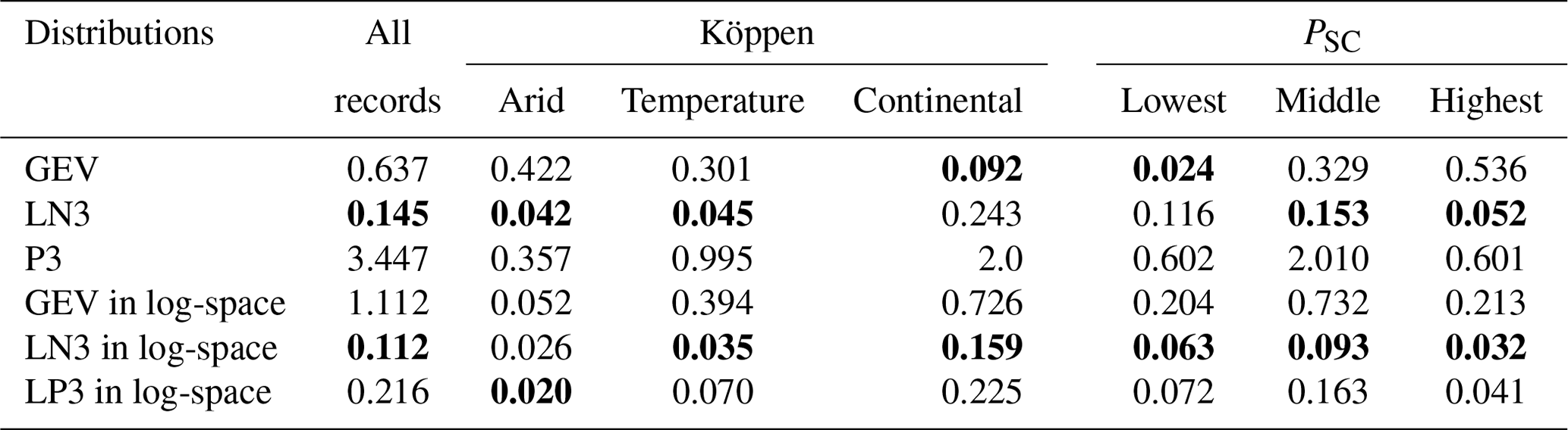
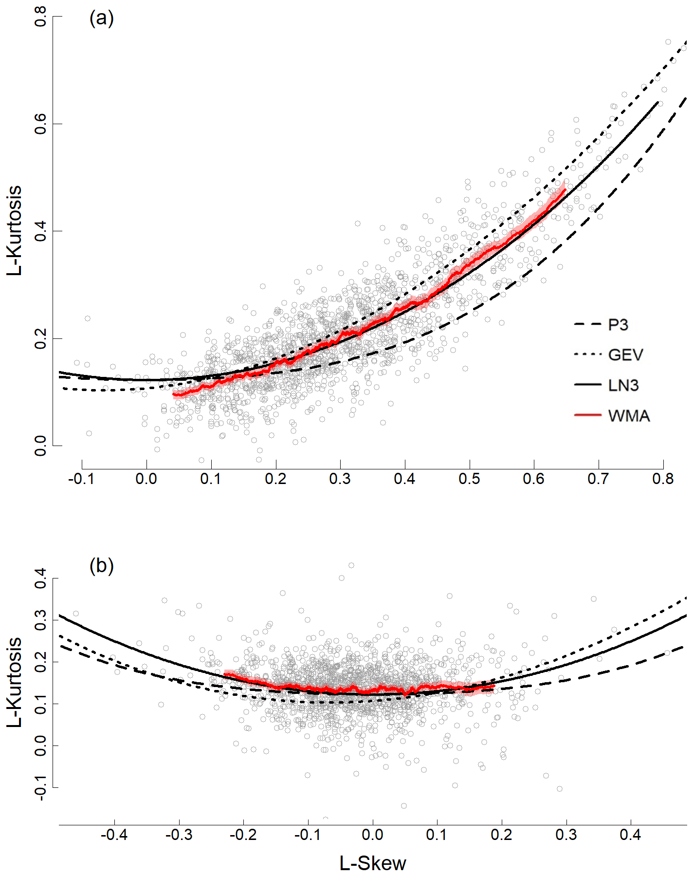
Figure 2 L-moment diagrams with the L-moment ratio for skew and kurtosis of annual maxima records used in this study (gray dots; n=1538), with their weighted moving average (WMA) proportional to record length (red line) and the P3, GEV, and LN distribution lines: (a) annual discharge maxima as recorded by gages and (b) the logarithm of the annual discharge maxima.

When annual maxima are grouped by Köppen climate region, the WMA shifts from the best-fitted distribution line as we move from arid to more temperate climates (Fig. 3). The statistical properties of records from temperate climates are best described by the LN3 distribution (Table 2; Fig. 3c), whereas records from continental regions are represented by a GEV distribution (Table 2; Fig. 3e). The WMA of annual records from arid climates does not track one distribution family line: the LN3 distribution best represents records with high L-skew values [0.5–0.7] and the P3 distribution better follows the lower L-skew values [0.1–0.4] (Fig. 3a). We note that the smaller sample size of the arid climate group results in larger confidence intervals. The concentrations of individual L-moment ratios also shift when grouped by climate region: the clustering of L-moment ratios for continental climates is highest along the GEV distribution line (Fig. 3e), for temperate L-moment ratios it falls in between the GEV and LN3 line (Fig. 3c), and for arid L-moments between the LN3 and P3 line (Fig. 3a). A clear shift between distribution families for different climate regions is not observed in log-space, with only small differences in the goodness-of-fit between the LP3 and LN3 distribution (Table 2). The log-transformed records in arid climates exhibit overall lower L-kurtosis values compared to records from continental and temperate climates and are best represented by the LP3 distribution for positive L-skew (Fig. 3b), whereas negative L-skew values do not clearly follow one distribution. Flood distributions in temperate regions are well represented by the LN3 distribution for negative L-skew values and by the LP3 distribution for positive L-skew values (Fig. 3d).

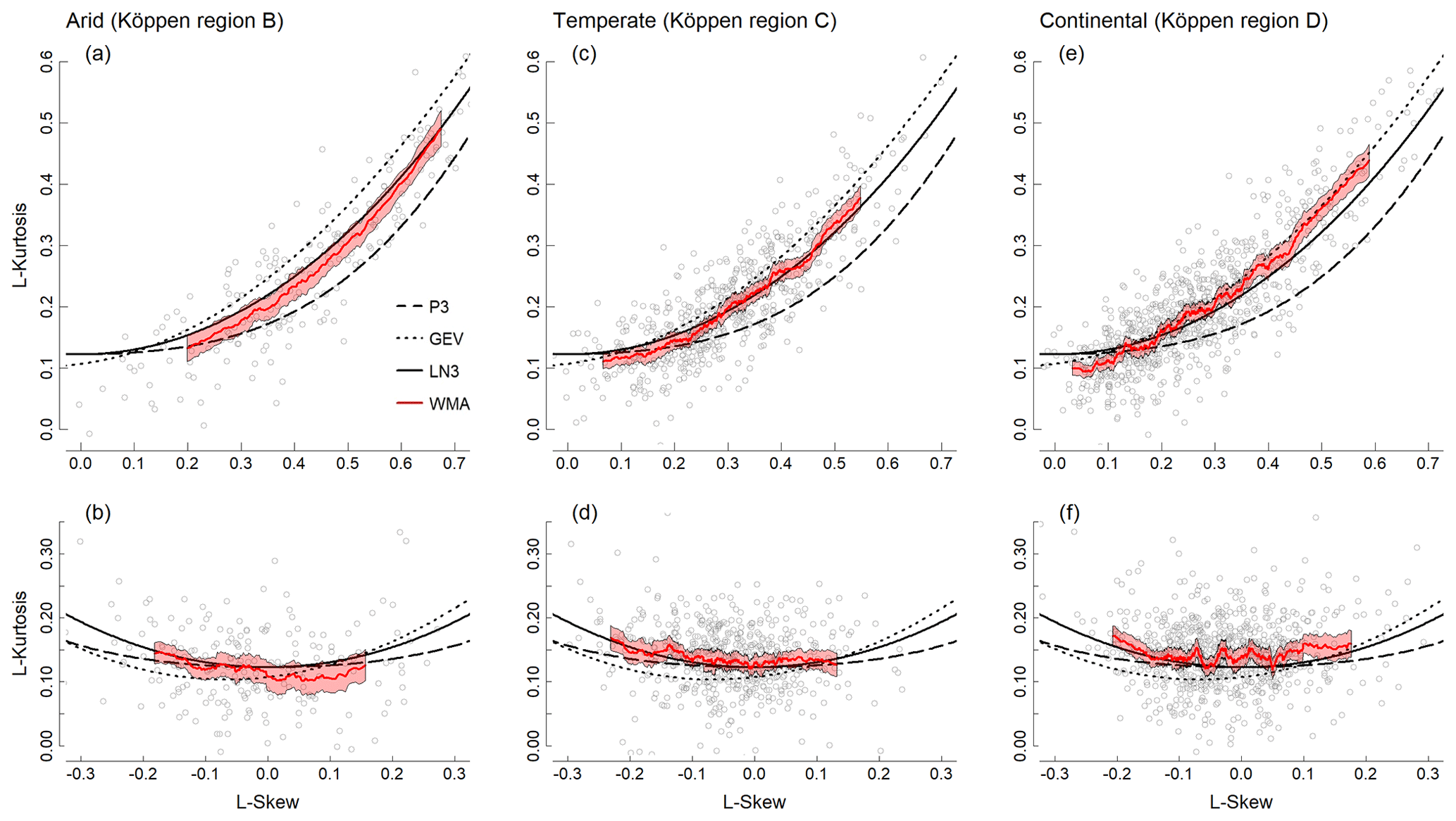
Figure 3 L-moment diagram with the L-skew and L-kurtosis for annual discharge maxima records (gray dots) grouped by their Köppen climate region, their weighted moving averages (WMA) proportional to record length (red line), and the P3, GEV, and LN distribution line (striped, dotted, solid). Panels (a), (c), and (e) show annual discharge maxima as recorded by the gage; panels (b), (d), and (f) show the logarithm of the annual discharge maxima.

Categorizing annual maxima discharge records based on different local precipitation intensities (P_SC) also influences the position and variance of the WMA (Table 2; Fig. 4). The WMA of records with low precipitation intensities follows the GEV distribution line (Table 2), especially for higher L-skew values [0.2–0.45] (Fig. 4a). The SSE scores indicate that the LN3 distribution best fits the L-moment ratios with high P_SC values (Table 2); however, along the range of L-skew values we do observe variation (Fig. 4e). The L-moment ratios associated with high P_SC values follow the LN3 distribution line for L-skew values between 0.4 and 0.7, whereas the WMA falls between the LN3 and P3 distribution for lower L-skew values [0.15–0.4] (Fig. 4e). The WMAs of the intermediate group fall in between the GEV and LN3 distribution lines, whereas for low [0–0.15] and high [0.4–0.6] L-skew values, it follows the GEV distribution. However, for intermediate L-skew values [0.15–0.4] it more closely follows the LN3 distribution (Fig. 3c). The position of this line within the parameter space indicates the observed shift from the GEV to the LN3 distribution as P_SC values increase (Fig. 4c). Additionally, the range of L-skew values is much smaller for records with low P_SC values (Fig. 4a). We could not clearly distinguish a best-fitted distribution between the groups when records were log-transformed (Table 2; Fig. 4b, d, and f). For the intermediate P_SC values the WMA line tracks the LN3 distribution line, but for the highest P_SC values the WMA follows both the LN3 distribution (for negative L-skew values) and the P3 distribution (for positive L-skew values).

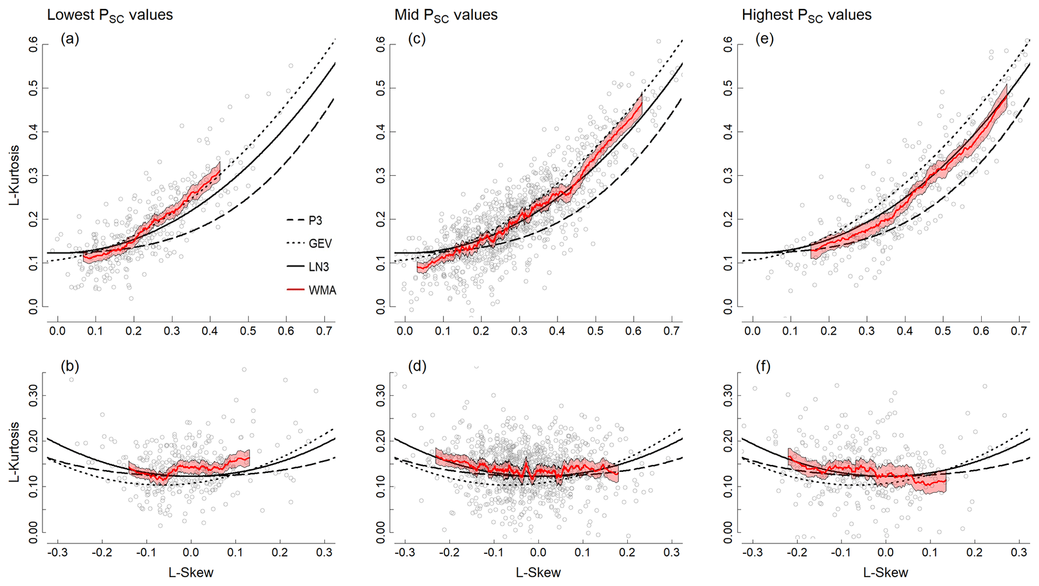
Figure 4 L-moment diagram with the L-skew and L-kurtosis for gage discharge records (gray dots) grouped by their percentage of the maximum annual daily precipitation level to the total annual precipitation level (P_SC), their weighted moving averages (WMA) proportional to record length (red line) and the P3, GEV, and LN distribution line. Panels (a), (c), and (e) show annual discharge maxima as recorded by the gage; panels (b), (d), and (f) show the logarithm of the discharges.

Our analyses document shifts in flood distribution properties for both the Köppen climate groups and the P_SC groups, where arid climates (high P_SC) and continental climates (low P_SC) move away from the LN3 distribution towards the P3 and GEV distribution. In contrast, the WMAs of both the temperate and intermediate P_SC group trend closer to the LN3 distribution line. A major difference between these two categories is the range of L-skew values between the corresponding groups. For example, the range of the lower P_SC is smaller than that of the L-moment ratios in continental climates. There is no clear best-fit distribution within the arid Köppen category and the higher P_SC groups, as the WMA varies over the observed L-skew range. However, we do demonstrate that regional hydroclimatic differences explain part of the variance among individual flood distributions.

4 Discussion

The main objective of this study is to evaluate whether hydroclimatic data can improve extreme flood probability estimates in flood frequency analysis procedures, through informed distribution family selection. To do this, we grouped annual hydrologic maxima from gage records across the United States by their hydroclimatic properties, and used L-moments to guide the selection of a probability model. Our work provides insights into the hydroclimatic parameters that drive flood frequency distribution shape and demonstrates how to supplement conventional flood frequency analyses using hydrological information accordingly.

4.1 Flood frequency distributions in the United States

The LN3 distribution most closely fits the average statistical properties of annual hydrologic maxima across the United States (Table 2), although for records with low L-skew values [0.05–0.2] the GEV distribution fits better (Fig. 2a). These findings are consistent with, and further specify, the work of Vogel and Wilson (1996), who also used L-moment diagrams to conclude that the LN3, LP3, and GEV distributions are all reasonable representations of annual maxima across the United States. In log-space the LN3 distribution also provides the best fit (Table 2); however, the theoretical distribution lines are more aligned, making the LP3 distribution an appropriate choice, as recommended by Bulletin 17C for records with positive L-skew values. Bulletin 17C accounts for negatively skewed flood distributions by censoring potentially influential low floods (PILFs) that could lead to underestimation of extreme flood values (England et al., 2019).

Our analyses demonstrate that hydroclimatic factors, such as Köppen climate region and precipitation intensity, explain part of the L-moment ratios sample variance and flood frequency distribution shapes across the United States. The distribution family that best characterized hydrologic maxima shifts from the GEV towards the LN3 distribution as we move from cold and wet climates (Köppen group D) to warmer and drier climates (Köppen group B) (Fig. 3). The contribution of the annual maximum storm to annual total precipitation (P_SC) shows a similar pattern: watersheds with a lower maximum storm contribution are best captured by the GEV distribution and those with a higher P_SC by the LN3 distribution (Fig. 4). Although we do not provide evidence for a causal link, the flood regimes generally associated with arid and continental hydroclimatic regions match the statistical properties of the GEV and LN3 distribution families as described by the L-moment lines (Figs. 3 and 4). For example, arid climates generally experience flash floods (high P_SC values) and as a result skewed flood frequency distributions (thick tails) compared to continental climates; similarly the LN3 distribution line fits higher L-skew ratios for the same L-kurtosis compared to the GEV distribution (Metzger et al., 2020; Zaman et al., 2012). It also fits the results of a simulation experiment by Salinas et al. (2014a) that shows how the high variance of the L-moment ratio samples cannot alone be attributed to sampling error and that other covariates were needed to explain the variance. They observed a shift in the best-fit distribution from GEV to LN3 as the total annual precipitation decreases over a catchment observed by Salinas et al. (2014b) in Europe. Köppen climate regions could provide a potential explanation for why Salinas et al. (2014b) found the GEV distribution to be the best fit for European annual maxima, as it is a continent dominated by temperate and cold climates (Köppen groups C and D). In contrast, the United States includes large regions with arid climates as well as temperate and cold regions, which shifts the overall best fit distribution for annual maxima to the LN3 distribution.

4.2 Improvements to flood frequency analysis

Even though watershed-specific hydroclimatic variables, such as main Köppen group, affect the variance of L-moment ratios of annual maxima records, they did not always yield a distinct best-fit distribution family for the constructed hydroclimatic regions in this study (Fig. 3). The Köppen classification indirectly already includes several flood-generating variables – precipitation seasonality and intensity, vegetation, soil type, infiltration capacity, and surface runoff levels – as they are constructed from temperature and precipitation levels (Kottek et al., 2006; Peel et al., 2007). Accordingly, the observed results for gages grouped by Köppen climate regions are likely confounded by any of these factors, including P_SC. As these climate classification schemes indirectly contain multiple environmental variables and encompass large contiguous areas they form a promising tool for systematic distribution selection in flood frequency analysis. Solely local precipitation intensities (like P_SC) may represent large river systems poorly if discharge at given downstream location is influenced by multiple precipitation regimes from multiple tributaries. Encountering this problem becomes less likely with Köppen regions which often cover entire watersheds. Yet, the high precipitation intensity (P_SC levels) group and the arid Köppen region generate multiple best-fitted distribution families across the range of possible L-skew values, implying that a more detailed classification is necessary. The annual maxima records in arid climates (Fig. 3a) and with intense precipitation regimes (high P_SC values) (Fig. 4e) are best-fitted either to the P3 distribution for low L-skew values or to the LN3 for high values. In this particular case, Köppen's specification for arid climates – BWh, BWk, and BSk – might provide a systematic method to distinguish between different types of arid regions. Additionally, one could include other basin characteristics, specifically geomorphic properties of the watershed (e.g., size and elevation) in further improving probability model selection, given that prior work points to hydroclimatic variables as exerting a primary control on flood distributions (Salinas et al., 2014b). For example, Pitlick (1994) showed that the shape parameter of flood frequency distributions in mountainous areas of the western United States were affected by regional precipitation intensity – combining climatic and geomorphic parameters.

Our main finding – that hydroclimatic properties of a basin exert a strong influence on the distribution of annual discharge maxima – provides a potential means to improve the accuracy of extreme flood probability estimates without altering the mathematical procedure described in flood frequency analysis guidelines like Bulletin l7C (England et al., 2019). One approach to further improve on our work is the weighted mixed populations framework, where one stratifies data and fits a parametric distribution to each new data population to aggregate the population distributions into a single distribution weighted on population size (Barth et al., 2019). In a hydrologic context, one could subdivide annual flood discharges based on different (periodic) flood-generating mechanisms. Accordingly, this method works particularly well for watersheds with multiple distinct flood-generating mechanisms, for example due to periodic atmospheric rivers, and skewed flood distributions (Barth et al., 2019). Another approach is to use other parametric distributions, with four or more parameters – although such methods do not explicitly consider hydrologic information – or a metastatistical extreme value distribution (MEVD) (Marani and Ignaccolo, 2015; Miniussi et al., 2020). An MEVD derives an extreme (annual maxima) flood frequency distribution via “ordinary” discharge values and has shown to be efficient with all sorts of parametric distributions (Marani and Ignaccolo, 2015).

5 Conclusions

We evaluated annual hydrologic maxima distributions from across the United States and showed that probability model selection can be improved when it is based on the hydroclimatic properties of the basin. In the United States, the WMA line of L-moment coefficients track the LN3 distribution, implying that this distribution could serve as a national distribution family. However, distribution selection can be improved by taking a basin's climate region into account, where continental climates (cool/wet) are best described by GEV distributions, while arid climates (hot/dry) are best described by LN3 distributions. More broadly, our work demonstrates that the climatology of a region is a powerful tool for guiding a priori distribution selection in flood frequency analysis.