the Creative Commons Attribution 4.0 License.
the Creative Commons Attribution 4.0 License.
 | 07 May 2024
Assessing downscaling techniques for frequency analysis, total precipitation and rainy day estimation in CMIP6 simulations over hydrological years
David A. Jimenez
Ariele Zanfei
Eber José de Andrade Pinto
Bruno Brentan
General circulation models generate climate simulations on grids with resolutions ranging from 50 to 600 km. The resulting coarse spatial resolution of the model outcomes requires post-processing routines to ensure reliable climate information for practical studies, prompting the widespread application of downscaling techniques. However, assessing the effectiveness of multiple downscaling techniques is essential, as their accuracy varies depending on the objectives of the analysis and the characteristics of the case study. In this context, this study aims to evaluate the performance of downscaling the daily precipitation series in the Metropolitan Region of Belo Horizonte (MRBH), Brazil, with the final scope of performing frequency analyses and estimating total precipitation and the number of rainy days per hydrological year at both annual and multiannual levels. To develop this study, 78 climate model simulations with a horizontal resolution of 100 km, which participated in the SSP1-2.6 and/or SSP5-8.5 scenarios of CMIP6, are employed. The results highlight that adjusting the simulations from the general circulation models by the delta method, quantile mapping and regression trees produces accurate results for estimating the total precipitation and number of rainy days. Finally, it is noted that employing downscaled precipitation series through quantile mapping and regression trees also yields promising results in terms of the frequency analyses.
- Article
(3333 KB) - Full-text XML
- BibTeX
- EndNote


As emphasized by the Intergovernmental Panel on Climate Change (IPCC), global climate models (GCMs) represent the most advanced climate simulation tools and play a fundamental role in evaluating future climate scenarios (IPCC, 2014). GCMs have the capability to generate coherent climate estimations both physically and geographically. The GCMs are used to examine the effect of increasing greenhouse gas emissions on climatic variables (Ostad-Ali-Askari et al., 2020). However, due to their low spatial resolution (50–600 km), they are unable to adequately reproduce the climatic variables of small areas such as basins and subbasins (Ozbuldu and Irvem, 2021), whereby the application of downscaling techniques has become a standard procedure (Worku et al., 2021; Olsson et al., 2016).
Downscaling aims to refine low-resolution global climate projections to local or regional scales by identifying relationships between observed climate data and simulations from GCMs (Jimenez, 2022; Zhang and Li, 2020). Downscaling enhances the representativeness of projected climate conditions, making them more accurate for local climate conditions. Ensuring adequate downscaling is essential since adjusted series are employed to assess the impacts of climate change on regional scales (Teutschbein et al., 2011). If an inadequate methodology of downscaling is selected for future climate projections, misinterpretation and inaccurate estimation of the effects of climate change, with detrimental consequences for long-term planning in the management of climate change impacts, could be made (Rastogi et al., 2022). For instance, underestimating regional-scale responses to climate change can result in a lack of preparedness from a planning and mitigation perspective. Conversely, overestimating these responses can lead to an excessive budget allocation for addressing the consequences.
Given the variety of downscaling techniques available in the literature (delta method, quantile mapping, machine learning techniques, etc.), Rastogi et al. (2022), Yang et al. (2019) and Onyutha et al. (2016) report that the efficiency of downscaling techniques varies for several reasons, such as the research objectives, the data and the case study, making it necessary to evaluate multiple techniques in each specific study. The analysis and characterization of changes in precipitation patterns is one of the most relevant thematic areas in research addressing the impacts of climate change. Mahla et al. (2019), Salehnia et al. (2019), Yang et al. (2019), Sachindra et al. (2018a) and Hashmi et al. (2011) evaluated the performance of downscaled techniques in reducing precipitation. Mahla et al. (2019) indicated that downscaling monthly precipitation based on multiple linear regressions showed promising results for the study area. On the other hand, Salehnia et al. (2019) identified that dynamic downscaling (DDS) provides better results than statistical downscaling (SDS) in total annual and seasonal precipitation downscaling, pointing out that SDS is computationally simpler than DDS. Conversely, Yang et al. (2019) found that methods based on quantile mapping demonstrate better performance in the downscaling of seasonal-scale and extreme precipitation compared to the function transform method (CDF-t). Sachindra et al. (2018) recommended using a regional vector machine (RVM) over genetic programming (GP), artificial neural networks (ANNs) and support vector machines (SVMs) for monthly precipitation downscaling. Finally, Hashmi et al. (2011) identified that GP provides better results for daily precipitation downscaling than ANNs.
Most of the studies have focused on assessing the efficiency of downscaling techniques for monthly, annual and seasonal precipitation by the civil year (Kreienkamp et al., 2019; Ozbuldu and Irvem, 2021). However, only a few studies have been conducted for the hydrological year. Instead, no studies were identified that evaluated the effectiveness of these techniques for conducting frequency analysis. Tabari et al. (2021), Liu et al. (2020), Norris et al. (2020) and Hassanzadeh et al. (2014) indicated that climate change could transform or modify temperature and relative humidity patterns, leading to the intensification of extreme weather events (Roca et al., 2019). Thus, authors such as Fadhel et al. (2017), Shahabul and Elshorbagy (2015) and Waters et al. (2003) emphasize that, in the current context of climate change, it is necessary to identify potential changes in intensity–duration–frequency (IDF) relationships.
Therefore, it is essential to assess the representativeness of downscaling techniques for conducting frequency analyses, because the number of studies evaluating the alterations in IDF relationships in the climate change context from simulations of GCMs has been increasing (e.g., Ghasemi Tousi et al., 2021, Hassanzadeh et al., 2014, or Hashmi et al., 2011). The assessment of changes in IDF relationships in climate change scenarios plays a fundamental role in decision-making related to the planning of hydraulic infrastructure, drainage systems, flood prevention and water resource management. Identifying these changes enables authorities, engineers and planners to incorporate new climate realities into the development of infrastructure projects.
To ensure accurate downscaling and to enable a correct estimation and interpretation of the impacts of climate change on IDF relationships, the proposed work aims to investigate the performance of some of the most recognized downscaling techniques in the literature, such as the delta method (DM), quantile mapping (QM) and regression trees (RT), in terms of frequency analysis. Additionally, the techniques were also evaluated for their ability to reproduce total precipitation and the number of rainy days per hydrological year and at a multiyear level. In this way, the present study contributes to the identification and selection of downscaling techniques that can be applied in research that assesses changes in IDF relationships from CMIP6 projections as well as in studies evaluating changes in the number of rainy days and total precipitation at the multiyear level in the context of climate change. In order to facilitate the paper's understanding, the second section presents the study area, the data used, the downscaling techniques considered and the efficiency metrics used to evaluate the downscaling techniques. The third section presents the results and discussion, while the fourth section draws the conclusions and final considerations.
2.1 Study area and historical rainfall records
The study was conducted in the Metropolitan Region of Belo Horizonte (MRBH), which is located between latitudes 18.0 and 20.5° S and between longitudes 43.15 and 44.75° E in the central region of the state of Minas Gerais, Brazil. The MRBH covers an area of 9468 km2 with a hydrological year starting in October, with precipitation occurring from October to March. Monthly precipitation can exceed 300 mm month−1. The MRBH monitoring network comprises more than 120 pluviometric stations distributed throughout the region (see Fig. 1a). The MRBH is selected because, as Nunes (2018) indicated, a significant portion of the MRBH is directly or indirectly experiencing the consequences of extreme rainfall events. Between 1928 and 2000, 200 floods were recorded in Belo Horizonte, with 69.5 % of these events occurring in the last 2 decades analyzed. Furthermore, over 37 flood events were reported between 2000 and 2020.
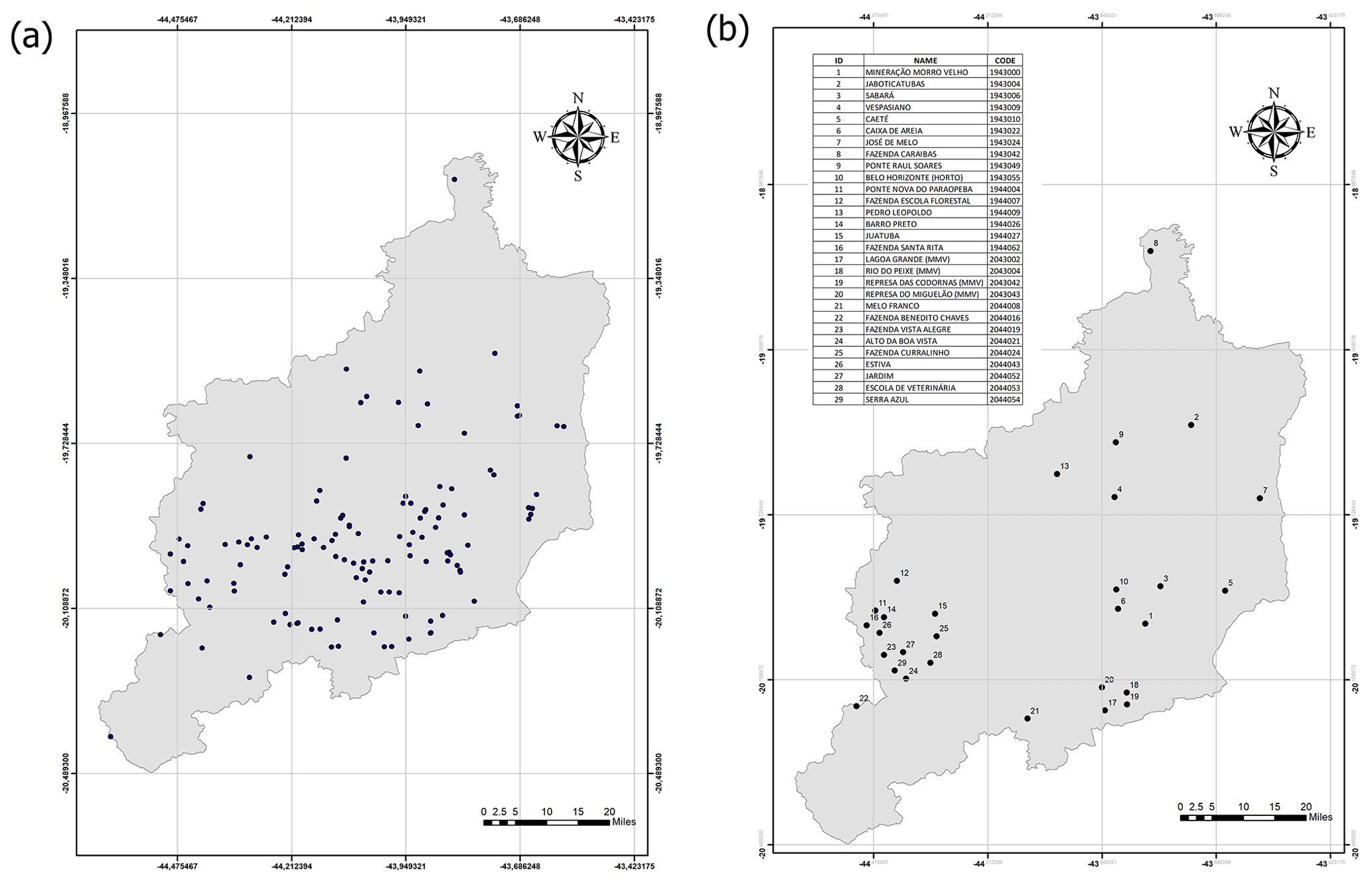
Figure 1Pluviometric stations of the MRBH: (a) monitoring network of pluviometric stations and (b) selected pluviometric stations used in the present study.
The rainfall records for the MRBH are obtained from the Hydrological Information System (Hidroweb) of the Brazilian National Water Agency, available at https://www.snirh.gov.br/hidroweb/serieshistoricas (last access: 31 March 2024). Upon downloading the rainfall data, we ensured their consistency by constructing double mass curves using the total precipitation data for each hydrological year. Rainfall stations with over 30 years of consistent records and with missing data below 10 % were selected. It is important to note that we did not fill in any missing data, as this could introduce uncertainties into the results. Double mass curves are processed to perform consistency analysis of the collected data. Stations with distances less than 44 km and a correlation equal to or greater than 0.7 from each reference station were selected to perform this calculation. It was evident that only 29 stations have more than 30 years of consistent records and missing data below 10 %. Thus, the study was developed from the rainfall information of the 29 stations shown in Fig. 1b.
2.2 Simulation of rainfall conditions
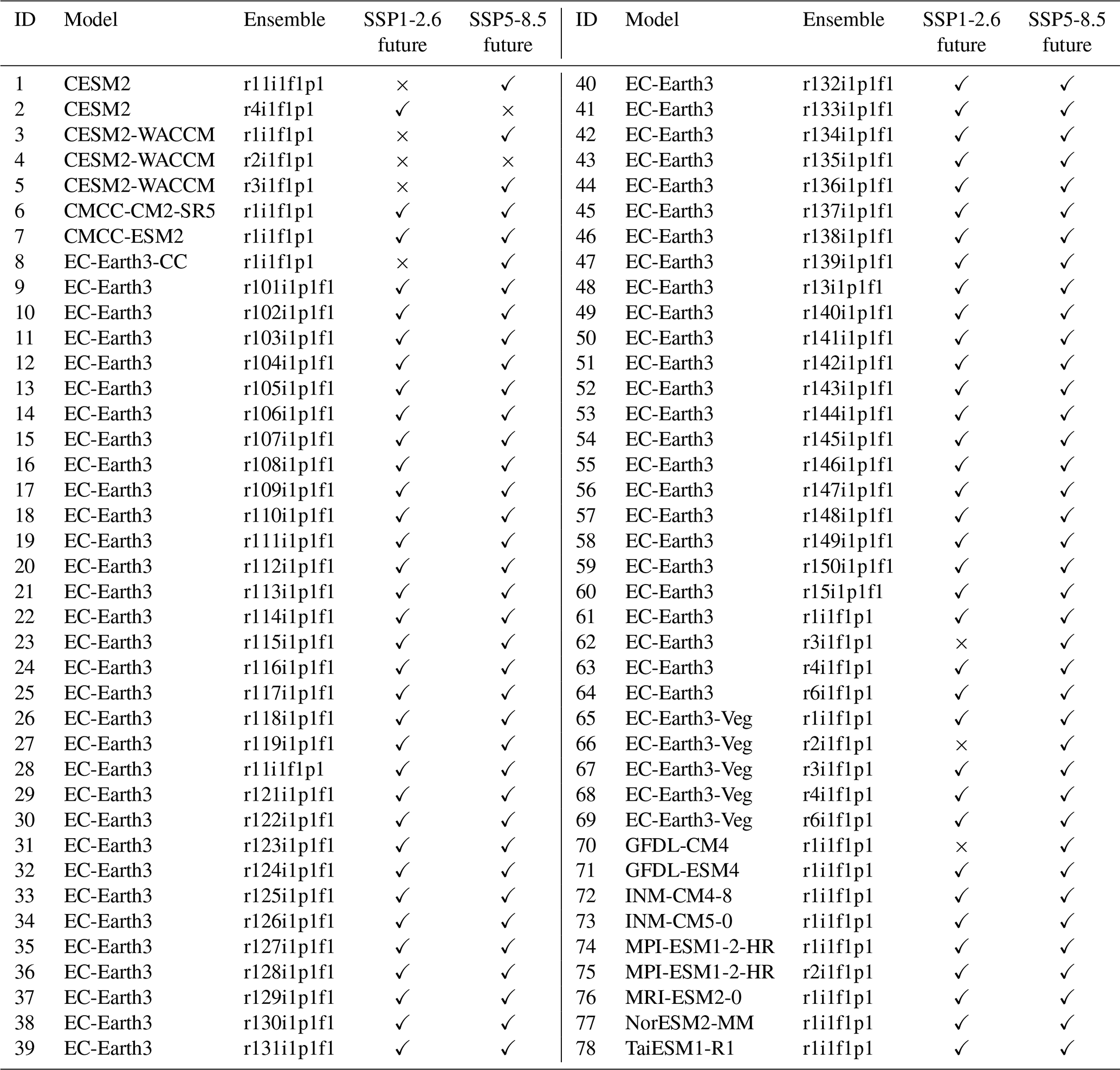
The daily precipitation data simulated for the historical period (1850–2014) by GCMs with a resolution of 100 km, participating in emission scenarios SSP1-2.6 and/or SSP5-8.5 of CMIP6, were obtained from https://esgf-node.llnl.gov/search/cmip6/ (last access: 31 March 2024). It is important to emphasize that all available simulations with a resolution of 100 km have been included to consider all the ensembles available for each climate model. This choice was made with the intention of utilizing all available model outputs and thus providing a more robust analysis.
The SSP5-8.5 and SSP1-2.6 scenarios are selected as the CMIP6 scenarios that project the highest and lowest temperature increases, respectively. In the case of the SSP5-8.5 scenario, it is assumed that the economic and social development of humankind until the end of the 21st century will be governed by (i) high exploitation of resources, (ii) intensive use of fossil fuels and (iii) high global energy demand. All these factors lead to high greenhouse gas concentrations, resulting in a radiative forcing of 8.5 W m−2 by the end of the 21st century (Riahi et al., 2016). On the other hand, the SSP1-2.6 scenario considers that (i) the world is turning towards sustainability, (ii) there is a commitment by nations to reduce social inequalities, and (iii) consumption is oriented towards low material growth and low resource and energy consumption. All these factors were combined with a radiative forcing of 2.6 W m−2 (Riahi et al., 2016). The simulations contemplated are presented in Table 1.
Table 1Overview of the CMIP6 GCM ensemble used in this study (r – realization or ensemble member; i – initialization method; p – physics; f – forcing).
2.3 Downscaling
The primary approaches to downscaling are SDS and DDS. In this study, two of the most popular SDS techniques were evaluated: the delta method, quantile mapping and the ML method regression trees. Due to their simplicity and low computational effort, the DM and QM have been widely used in many research studies. In the case of the DM, the investigations developed by Salehnia et al. (2020, 2019) and Teutschbein and Seibert (2012) are noteworthy. The study developed by Salehnia et al. (2020) aims to investigate the impact of climate change on rainfed wheat yield in Khorasan-e Razavi Province of northeastern Iran. The study used climate projections from GCMs to assess the potential impact of climate changes on rainfed wheat yield over the next decades (2019–2038).
The DM was used to correct the simulations of temperature and precipitation on the daily and monthly scales. On the other hand, Salehnia et al. (2019) compared the performance of the DM and DDS in terms of the amount and number of wet days and total precipitation at the annual and seasonal scales. The results showed that DDS has better performance than the DM. Similarly, it is highlighted that the DM underestimates the annual mean precipitation and the number of wet days, while DDS overestimates them. Finally, Teutschbein and Seibert (2012) compared the performance of different downscaling techniques to correct precipitation and temperature. Their results highlighted that the delta method is a stable and robust method, with the ability to produce future time series with dynamics similar to current conditions. However, the method does not consider potential changes in future climatic dynamics.
With respect to QM, the studies conducted by Enayati et al. (2021), Heo et al. (2019) and Themeßl et al. (2011) are noteworthy. In the study conducted by Enayati et al. (2021), the capability of bias correction in precipitation and temperature simulations of GCMs using the QM technique was evaluated. The results indicated that nonparametric methods of quantile mapping exhibited the best performance. On the other hand, Heo et al. (2019) evaluated the use of different probability distributions in QM, and the results showed that the selection of the probability distribution could lead to better or worse results. Finally, Themeßl et al. (2011) indicated that the use of quantile mapping has better performance in the estimation of high quantiles. In this way, the use of this technique could present an advantage in the case of extreme precipitation events.
In the case of RT, the studies conducted by Khalid and Sitanggang (2022) and Hutengs and Vohland (2016) stand out. Khalid and Sitanggang (2022) compared various ML methods for downscaling precipitation, showing that RT performed best. On the other hand, the study conducted by Hutengs and Vohland (2016) adopted RT to enhance the spatial resolution of temperature based on land surface temperature and reflectance with favorable results.
A pixel–station downscaling approach was developed. Observational data from each station were collected along with simulated GCM data, extracted from the pixel containing that station. For all the selected pairs of time series, the temporal consistency between daily precipitation observed and simulated was guaranteed by selecting the simulated data only for the day on which the observation data are presented. Once the simulated series was obtained, the evaluated downscaling techniques were applied for each selected point.
2.3.1 Delta method
In this method, differences or “deltas” between observed and GCM-simulated climatic conditions in the historical period are calculated. Subsequently, assuming that these differences or deltas remain constant over time, they are applied to GCM-simulated future climate projections, thus refining climate projections at local or regional levels. The mathematical equation employed by the delta method is presented below:
where represents the downscaled precipitation, PMod,daily represents the simulated precipitation by the GCMs, represents the average monthly precipitation of the station, and represents the average monthly precipitation simulated.
2.3.2 Quantile mapping
QM is based on the principle of matching the quantiles of observed and GCM-simulated distributions. The process begins with estimating the quantiles of the observed series. Then, for the future period, the empirical probability associated with the quantile simulated by the GCMs is estimated. This probability is used in the inverse probability function of observed quantiles, thus obtaining the downscaled value. The following is a mathematical description of the method of precipitation:
where is the precipitation with downscaling, is the inverse empirical probability function of daily precipitation for the historic period, FM is the empirical probability function of simulated precipitation, and PM is the simulated precipitation.
2.3.3 Regression trees
Regression trees are a machine learning technique used to build predictive models. These models are created by recursively dividing the sample space and adjusting predictive models for each subdivision (Loh, 2011). The main goal of this technique is to partition the sample space into k units and to create a predictive model for each subspace. This approach enables the prediction of the variable of interest, Y, using a piecewise function of the type
where Y is the predicted variable, is the predictive model of the sample subspace Ei, and x is the predictor variable. Downscaling using RT can incorporate more than one predictor variable to estimate the variable of interest. For example, precipitation could be estimated using multiple variables simulated by general circulation models, such as temperature, atmospheric pressure and precipitation. However, it is important to note that the uncertainties in downscaling tend to increase with the number of predictors. In this way, only daily precipitation is simulated as the predictor variable to minimize these uncertainties. The downscaling process was carried out using observed and simulated precipitation quantiles. This approach is used due to the absence of a consistent temporal correlation between the observed and simulated rainfall magnitudes. Often, the simulated precipitation by the GCMs did not match with the historical records, leading to instances where GCMs projected rainfall on days when historical data indicated dry weather conditions. In the training stage, 85 % of the records were used, while in the validation stage, 15 % were employed. The optimization of hyperparameters (maximum number of splits, split criterion) was conducted using the automatic hyperparameter optimization function available in the fitrtree function in MATLAB.
2.4 Frequency analysis
The frequency analysis is carried out using the maximum annual precipitation series estimated from both historical records and downscaling results. Initially, the stationarity and homogeneity of the maximum series are confirmed using the Spearman (NERC, 1975) and Mann–Whitney (1947) statistical tests. These tests are applied at a 5 % significance level as specified by Naghettini and Pinto (2007). The frequency analysis is exclusively conducted on the series that exhibited homogeneity and stationarity. This analysis considered various probability distributions, including exponential, gamma, Gumbel, generalized extreme value (GEV) distribution, log-normal, Pearson III and log-Pearson III. The parameters for these distributions are estimated using the L-moments method (Hosking and Wallis, 1993). To evaluate the adherence of the series to these probability distributions, the nonparametric Kolmogorov–Smirnov test is applied at a significance level of 5 %. For each station, the quantiles of precipitation associated with return periods of 2, 5, 10, 15, 30, 35, 45, 50, 60, 70, 80, 90 and 100 years were estimated based on the distribution with the best fit.
2.5 Comparison between estimates made with historical series and downscaling
The efficiency of downscaling techniques was assessed in terms of total precipitation (TP) and the number of rainy days (RDs) at both the hydrological-year and multiyear levels. In the latter case, the total precipitation and rainy days are aggregated over the available record period. Similarly, the techniques are examined in terms of frequency analysis.
The TP and RD by the hydrological year are evaluated using the Nash–Sutcliffe efficiency (NSE), Kling–Gupta efficiency (KGE), root-mean-square error (RMSE) and Pearson correlation coefficient (R). In the case of the multiyear level, the evaluation was performed using the percentage error. Nash and Sutcliffe (1979) and Gupta et al. (2009) indicated that NSE and KGE values of 1 represent an ideal match between observed and simulated data. In the case of the RMSE, a value of 0 signifies a perfect fit. Moreover, the R value, which falls between 0 and 1, indicates a positive correlation. Values between −1 and 0 suggest a negative correlation, while those near 0 imply no correlation. Finally, a percentage error value of 0 indicates a perfect fit between observed and simulated data. The equations used to calculate the NSE, KGE, RMSE, R and percentage error are provided below:
where Xi and are the observed and simulated values, while and are the mean of the observed and simulated values, respectively. n represents the number of simulated data, the standard deviation of the simulated values, σi the standard deviation of the observed records and R the correlation coefficient between the observed and simulated records.
3.1 Total precipitation and number of rainy days per hydrological year
Seventy-eight analyses were conducted for both total precipitation for the hydrological year and the number of rainy days, and the median values of NSE, KGE, RMSE and R were computed to facilitate the analysis and interpretation of the results, emphasizing that the median was chosen because it is less susceptible to extreme events.
Number of rainy days per hydrological year
Estimating the number of rainy days in the hydrological year from downscaled series using the DM, QM and RT methods yields unsatisfactory results in all the evaluated models. Thus, Fig. 2 and Table 2 reveal discrepancies in the number of rainy days estimated per hydrological year from the downscaled series compared to observations. Without the application of any downscaling technique (WDS), this difference is approximately 78 d.

Figure 2Median performance metrics (RMSE and R) for the estimated number of rainy days from precipitation series simulated by GCMs, without the application of downscaling techniques (WDS), as well as adjusted series obtained using the DM, QM and RT.
Table 2Summary of performance metrics for estimating the number of rainy days from without-downscaling and reduced series using the DM, QM and RT methods.
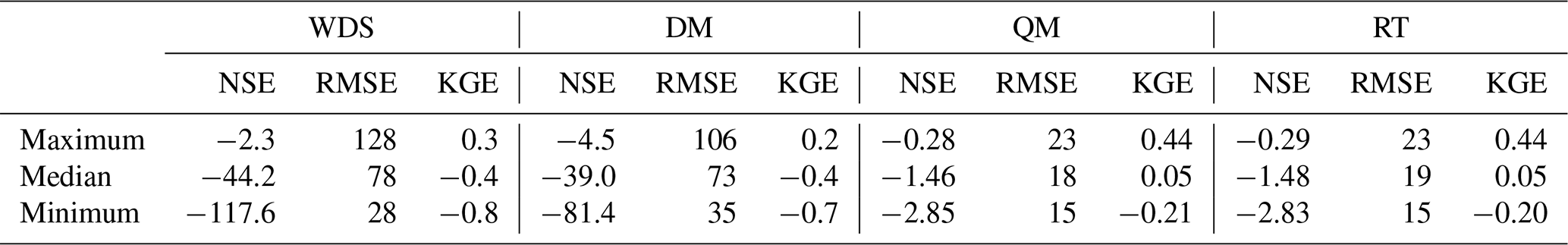

Figure 3Median percentage error of underestimation or overestimation of the total number of rainy days per hydrological year. The percentage error of the prevailing condition of underestimation (“Under.”) or overestimation (“Over.”) is represented in blue, while the non-prevailing condition is depicted in orange. For example, if underestimation is prevalent, overestimation is represented in orange. WDS represents the condition without the application of downscaling techniques, DM corresponds to the condition when the delta method is applied, QM represents the condition when quantile mapping is applied, and RT indicates the condition of applying regression trees as a downscaling technique.
However, when using the DM, QM and RT as downscaling techniques, the difference decreases to 73, 18 and 19 d, respectively. Thus, QM and RT stand out for providing the greatest reduction in the discrepancy between the number of rainy days per hydrological year estimated from the downscaled series compared to observations. Nonetheless, as mentioned and observed in Table 2 and Fig. 2, the low NSE, KGE and R scores show that the estimation of the number of rainy days at the annual scale does not work well.
As shown in Fig. 3, the low performance of the NSE and KGE observed in Table 2 in the estimation of the number of rainy days per hydrological year is associated with underestimations or overestimations.
As observed in Fig. 3, an underestimation of the number of rainy days occurs when no downscaling techniques are applied. This underestimation trend persists when the DM is applied, consistent with the results found by Salehnia et al. (2019). However, when using QM and RT, this trend reverses, resulting in overestimation. The persistence of underestimation when the DM is applied may be related to the method of applying a constant correction factor per month. On the other hand, the shift from underestimation to overestimation when using QM and RT can be attributed to the relationship between simulated and observed quantiles. Therefore, it is possible that there is a reclassification of dry days (P≤1.0 mm) as wet days (P>1.0 mm) (i.e., a simulated quantile of 0.2 mm can be associated with observed precipitation >1 mm). The median percentage underestimation errors were 85.21 %, 79.3 %, 14.50 % and 13.70 % for WDS, the DM, QM and RT, respectively. Meanwhile, the average overestimations were 12.54 % and 13.78 % for QM and RT, respectively.
Table 3Summary of performance metrics for estimating the total precipitation by hydrological year without downscaling (WDS) and with the DM, QM and RT methods.
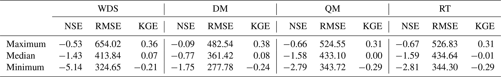
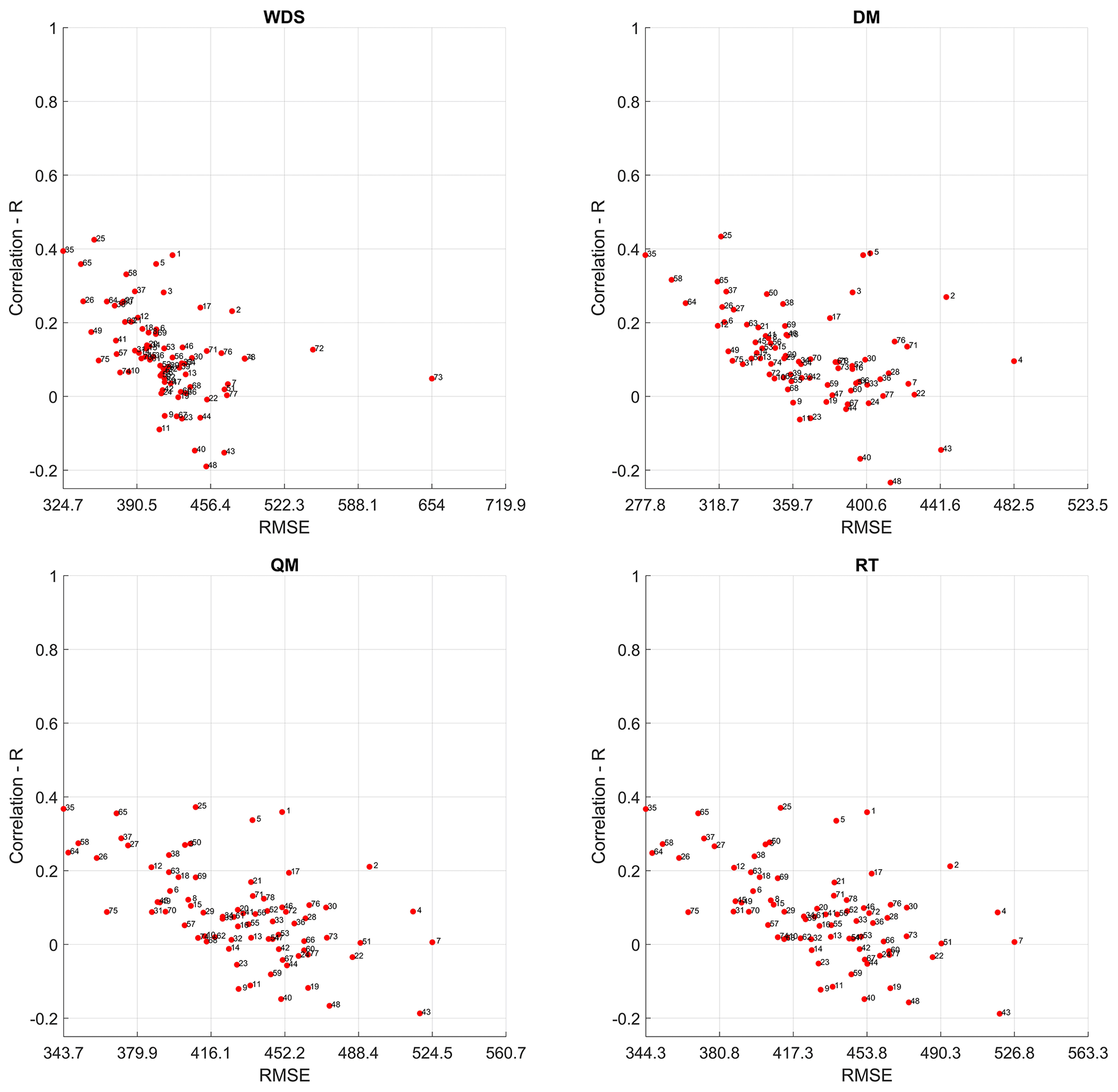
Figure 4Median performance metrics (RMSE and R) for estimated total precipitation from series simulated by GCMs, WDS and adjusted series obtained using the DM, QM and RT.

Figure 5Median percentage error of underestimation or overestimation of total precipitation per hydrological year. The percentage error of the prevailing condition of underestimation (“Under.”) or overestimation (“Over.”) is represented in blue, while the non-prevailing condition is depicted in orange. For example, if underestimation is prevalent, overestimation is represented in orange. WDS represents the condition without the application of downscaling techniques, DM corresponds to the condition when the delta method is applied, QM represents the condition when quantile mapping is applied, and RT indicates the condition of applying regression trees as a downscaling technique.
Total precipitation per hydrological year
Estimating the total precipitation per hydrological year from the downscaled series obtained through the application of the DM, QM and RT does not guarantee good results. Thus, when no downscaling technique is applied, the difference between the total precipitation estimated from the downscaled series differs, with a median of 413.84 mm. In the case where the DM is applied, this difference decreases to approximately 361.42 mm. However, when the QM and RT are applied, the differences are higher than when no downscaling technique is applied, with median differences of 433.10 and 434.64 mm, respectively (see Fig. 4 and Table 3). In that way, the difference between the total precipitation estimated from the downscaled series by the QM and RT increases by approximately 4 % compared to the estimations when no downscaling technique is applied and decreases by 12 % when the DM is applied. On the other hand, the low NSE, KGE and R scores, as shown in Fig. 4, indicate that the estimation of total precipitation at the annual scale from the downscaled series does not perform well.
In the same way as with the number of rainy days, the difference between the total precipitation per hydrological year estimated from observed data and downscaled data is associated with underestimations and overestimations. When no downscaling technique is applied, an underestimation of total precipitation per hydrological year is observed. However, when the DM, QM or RT is applied, this underestimation changes to overestimation (see Fig. 5).
In the case of QM and RT, the overestimation of total hydrological precipitation per year (Fig. 4) is related to the overestimation of the number of rainy days (Fig. 3) most of the time. Thus, it is noticeable that the application of QM and RT increases both the number of rainy days in the hydrological year and the magnitudes of simulated precipitations. However, this trend is intrinsic to the conceptual foundation of these methods. For example, during the application of QM or RT, a simulated quantile of 1 mm of rain can be associated with an observed quantile of 20 mm of rain. The median percentage underestimation errors were 25.58 %, 17,02 %, 18.74 % and 18.77 % for WDS, the DM, QM and RT, respectively. Meanwhile, the average overestimations were 22.37 %, 14.63 %, 18.37 % and 18.30 % for WDS, the DM, QM and RT, respectively.
3.2 Total precipitation and number of rainy days at the multiyear level
In the multiyear context, estimates derived from downscaled series using the DM, QM and RT showed more robust agreement with the estimations made from the historical records compared to the annual scale. A low discrepancy between the number of rainy days and total precipitation was observed at the multiyear scale.
When examining the number of rainy days, it was noted that the smallest errors are achieved when employing QM and RT as downscaling techniques. Additionally, estimates derived from downscaled series through the DM demonstrated a performance similar to cases where no downscaling technique was applied (see Fig. 6 and Table 4). Thus, at the multiyear scale, the series adjusted by QM yielded the smallest percentage errors, followed by those adjusted by RT and the DM.

Figure 6Median of percentage errors of rainy days at the multiyear level for each model. WDS and with the application of the DM, QM and RT as downscaling techniques.
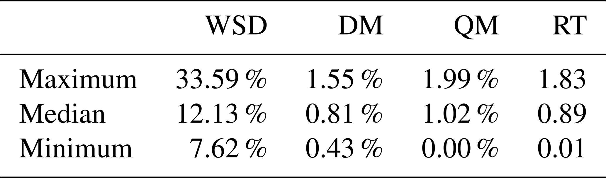
Table 4Summary of percentage errors of the number of rainy days at the multiyear level.

On the other hand, it was observed that the estimation of total precipitation at the multiyear scale from series downscaled by the DM, QM and RT significantly reduces percentage errors compared to cases where no downscaling technique is applied (see Fig. 7 and Table 5).
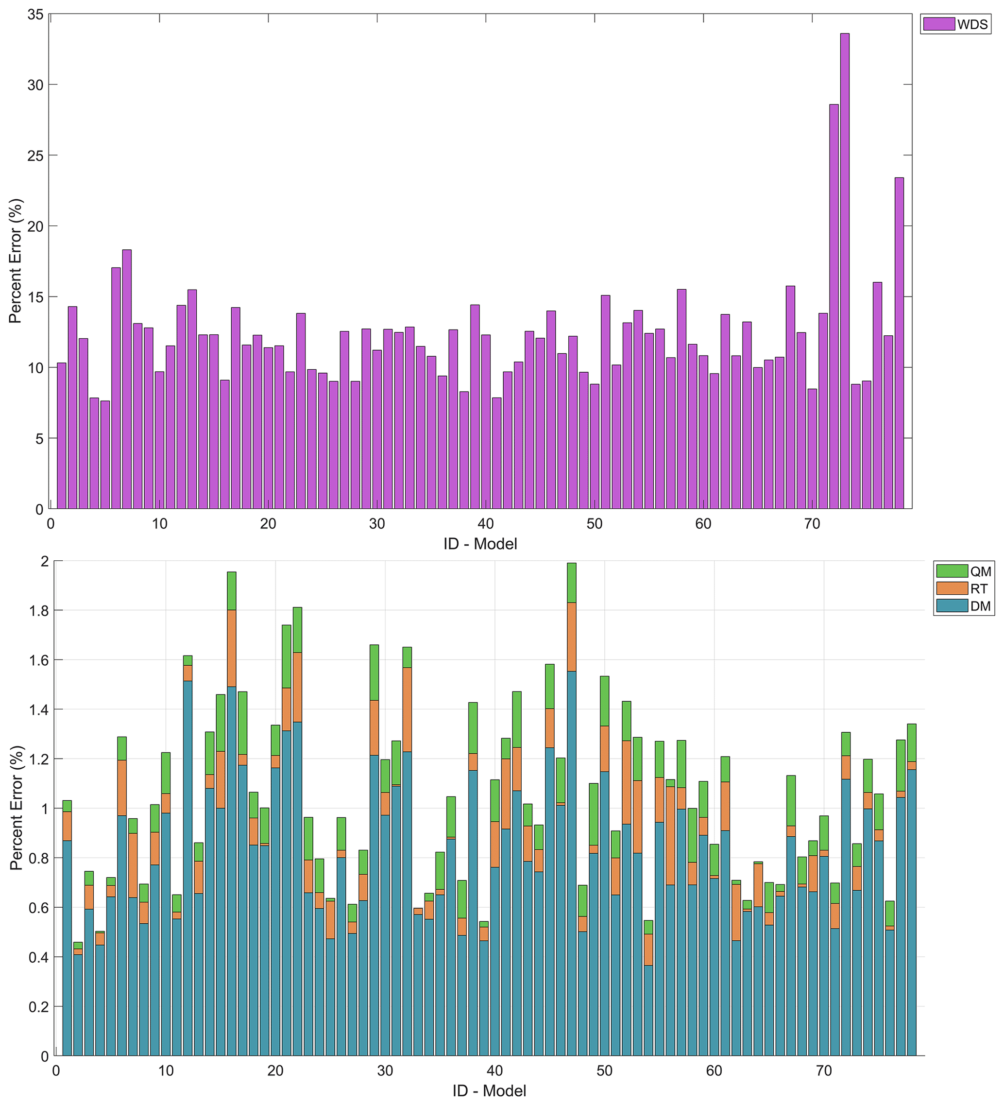
Figure 7Median of percentage errors of total precipitation at the multiyear level for each model. WDS and with the application of the DM, QM and RT as downscaling techniques.
Table 5Summary of the percentage errors of total precipitation at the multiyear level.
Based on the results, employing downscaled series for estimating total precipitation and the number of rainy days on a hydrological-year scale demonstrates better performance in the multiyear context. Therefore, it is recommended to utilize downscaled series by employing the DM, QM and RT for estimating total precipitation and the number of rainy days at the multiyear scale.
It was observed that the performance of downscaling techniques at the annual scale was consistently reflected at the multiyear scale. Regarding the number of rainy days, the QM method demonstrated superior performance across both the annual and multiyear scales. As for the total precipitation per hydrological year, the DM showcased the best performance, exhibiting even higher efficiency at the multiyear scale.
3.3 Frequency analysis
Developed frequency analyses from downscaled series using QM and RT yield satisfactory results, evidenced by good performance in the NSE and KGE metrics. With respect to the frequency analyses developed from series downscaled by the DM, it is observed that the results were comparable to those obtained when no downscaling technique was applied (see Fig. 8 and Table 6).

Figure 8Median performance metrics (NSE and KGE) for the frequency analysis developed from precipitation series simulated by GCMs, WDS and adjusted series obtained using the DM, QM and RT.
Table 6Summary of percentage errors obtained in the frequency analysis.
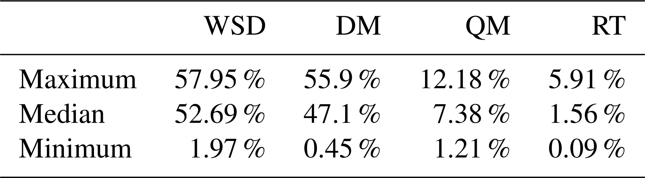
Figure 8 illustrates a significant improvement in yield metrics following the implementation of QM and RT. The metrics approach unity, suggesting that the quantiles estimated from the adjusted series closely align with those derived from the historical series. The percentage errors obtained in the estimates made with series downscaled by QM and RT were less than 12.18 % and 5.91 %, respectively. In contrast, the errors in the estimates made with series downscaled by the DM were similar to those obtained when no downscaling technique was applied (see Table 6 and Fig. 9).
The high performance achieved in the estimation of quantiles from adjusted series through QM and RT is associated with the fact that the largest quantiles simulated by GCMs are correlated with the largest observed quantiles. Consequently, observed and simulated series of maximum values end up with close values. This fact leads to comparable outcomes in estimations, regardless of whether they are derived from observed or downscaled series.
Given that downscaling in the case of the DM is accomplished through the application of factors, the difference between the maximum precipitation observed and estimated from the adjusted series is substantial. Consequently, this results in a significant disparity in the outcomes of frequency analyses. It was evident that the dispersion and variability of estimated quantiles from the adjusted series increased as the return period extended; however, this must be associated with the low occurrence of quantiles with high return times in the historical series (see Fig. 10). Additionally, it was observed that errors related to the DM are associated with an underestimation of quantiles for different return periods. Thus, it is concluded that the development of frequency analyses from adjusted series through QM and RT is feasible, with RT emerging as the technique that exhibited the best performance.

Figure 9Median of the percentage error obtained in the frequency analysis developed from precipitation series simulated by GCMs, WDS and reduced series obtained using the DM, QM and RT.

Figure 10Frequency analysis developed from precipitation series simulated by GCMs, WDS and adjusted series obtained using the DM, QM and RT for the return times of 2, 5, 10, 15, 25, 30, 35, 45, 50, 60, 70, 80, 90 and 100 years.
This study aimed to assess the performance of using downscaled series with the delta method, quantile mapping and regression trees to develop frequency analysis and estimate total precipitation and the number of rainy days per hydrological year at the annual and multiyear levels.
It was observed that the global climate models (GCMs) from the sixth phase of the Coupled Model Intercomparison Project (CMIP6) underestimated the number of rainy days per hydrological year for the MRBH, with a median of 78 d. When estimating the number of rainy days from the downscaled series by the DM, the tendency of underestimation persists and insignificantly decreases to 73 d. It was also observed that, when employing downscaled series through the application of QM and RT, underestimation is reversed to a slight overestimation. The average overestimations were 18 d for QM and 19 d for RT. Despite the relatively low magnitudes of the overestimations, the low NSE and KGE scores suggest that estimating the number of rainy days at an annual scale from the downscaled series using the DM, QM and RT does not guarantee accurate results.
Similarly, GCMs underestimate total precipitation for the hydrological year, with a median of 413.84 mm. The use of a downscaled series by the DM reduces this difference to 361.42 mm. However, when QM and RT are applied, the differences surpass those without downscaling. The median differences in those cases are 433.10 mm for QM and 434.64 mm for RT. These facts, along with the low NSE and KGE scores, suggest that annual estimations of the number of rainy days and total precipitation from downscaled series by the DM, QM and RT do not yield reliable results. This result is also due to the fact that a 1-year time window is not optimal for analyzing the precipitation simulated by the considered GCMs, and consequently more significant results were found with the multiyear study. Therefore, at the multiyear scale, the estimation of the number of rainy days and total precipitation demonstrated high performance. For the number of rainy days, the percentage errors between the magnitudes of the total estimated from adjusted and observed series were less than 1.21 % and 2.58 % when downscaled series by QM and RT were employed. Percentage errors for estimating total rainfall per hydrological year on a multiyear scale were 1.55 %, 1.99 % and 1.83 % when downscaled series by the DM, QM and RT, respectively, were used.
Finally, developing frequency analysis from the daily precipitation simulated by the GCMs allows quantiles close to those estimated with historical records to be obtained when QM and RT are applied. The performance achieved in estimating quantiles from adjusted series by QM and RT is attributed to the fact that QM and RT associate the largest quantiles simulated by GCMs with the largest observed quantiles. As a result, observed and downscaled series have close values. The percentage error of estimates made from downscaled series by QM and RT, in relation to estimates based on observed data, were lower than 12.18 % and 5.91 %, respectively. In this context, it is recommended to utilize downscaling based on RT when the goal is to assess future changes in the frequency of occurrence.
Some or all of the code that supports the findings of this study is available from the corresponding author.
Some or all of the data and models that support the findings of this study are available from the corresponding author.
DAJ and EJdAP conceptualized the research. DAJ, AM and AZ wrote the manuscript with the help of all the authors. BB designed the computational framework. DAJ, EJdAP and BB verified the analytical methods. All the authors provided critical feedback and helped shape the research, analysis and manuscript.
The contact author has declared that none of the authors has any competing interests.
Publisher's note: Copernicus Publications remains neutral with regard to jurisdictional claims made in the text, published maps, institutional affiliations, or any other geographical representation in this paper. While Copernicus Publications makes every effort to include appropriate place names, the final responsibility lies with the authors.
This work was supported by the Open Access Publishing Fund of the Free University of Bozen-Bolzano.
This paper was edited by Lelys Bravo de Guenni and reviewed by Kyunghun Kim and one anonymous referee.
Enayati, M., Bozorg-Haddad, O., Bazrafshan, J., Hejabi, S., and Chu, X.: Bias correction capabilities of quantile mapping methods for rainfall and temperature variables, J. Water Clim. Change, 12, 401–419, https://doi.org/10.2166/wcc.2020.261, 2021.
Fadhel, S., Rico-Ramirez, M. A., and Han, D.: Uncertainty of Intensity–Duration–Frequency (IDF) curves due to varied climate baseline periods, J. Hydrol., 547, 600–612, https://doi.org/10.1016/j.jhydrol.2017.02.013, 2017.
Ghasemi Tousi, E., O'Brien, W., Doulabian, S., and Shadmehri Toosi, A.: Climate changes impact on stormwater infrastructure design in Tucson Arizona, Sustain. Cities Soc., 72, 103014, https://doi.org/10.1016/j.scs.2021.103014, 2021.
Gupta, H. V., Kling, H., Yilmaz, K. K., and Martinez, G. F.: Decomposition of the mean squared error and NSE performance criteria: Implications for improving hydrological modelling, J. Hydrol., 377, 80–91, https://doi.org/10.1016/j.jhydrol.2009.08.003, 2009.
Hashmi, M. Z., Shamseldin, A. Y., and Melville, B. W.: Statistical downscaling of watershed precipitation using Gene Expression Programming (GEP), Environ. Modell. Softw., 26, 1639–1646, https://doi.org/10.1016/j.envsoft.2011.07.007, 2011.
Hassanzadeh, E., Nazemi, A., and Elshorbagy, A.: Quantile-Based Downscaling of Precipitation Using Genetic Programming: Application to IDF Curves in Saskatoon, J. Hydrol. Eng., 19943–19955, https://doi.org/10.1061/(ASCE)HE.1943-5584.0000854, 2014.
Heo, J.-H., Ahn, H., Shin, J.-Y., Kjeldsen, T. R., and Jeong, C.: Probability Distributions for a Quantile Mapping Technique for a Bias Correction of Precipitation Data: A Case Study to Precipitation Data Under Climate Change, Water, 11, 1475, https://doi.org/10.3390/w11071475, 2019.
Hosking, J. R. M. and Wallis, J. R.: Some statistics useful in regional frequency analisys, Water Resour. Res., 29, 271–281, https://doi.org/10.1029/92WR01980, 1993.
Hutengs, C. and Vohland, M.: Downscaling land surface temperatures at regional scales with random forest regression, Remote Sens. Environ., 178, 127–141, https://doi.org/10.1016/j.rse.2016.03.006, 2016.
IPCC: Climate Change 2014 Mitigation of Climate Change: Working Group III Contribution to the Fifth Assessment Report of the Intergovernmental Panel on Climate Change, Cambridge, Cambridge University Press, https://doi.org/10.1017/CBO9781107415416, 2014.
Jimenez, D. A.: Avaliação das alterações nas frequências de ocorrência das precipitações diárias máximas para a região Metropolitana de Belo Horizonte considerando diferentes cenários de climas futuros, Universidade Federal de Minas Gerais – UFMG, Belo Horizonte, http://hdl.handle.net/1843/46268 (last access: 31 March 2024), 2022.
Khalid, I. A. and Sitanggang, I. S.: Machine Learning-Based Spatial Downscaling on Precipitation Satellite Data in Riau Province, Indonesia, Turkish Journal of Computer and Mathematics Education, 13, 10, https://turcomat.org/index.php/turkbilmat/article/view/12114 (last access: 31 March 2024), 2022.
Kreienkamp, F., Paxian, A., Früh, B., Lorenz, P., and Matulla, C.: Evaluation of the empirical–statistical downscaling method EPISODES, Clim. Dynam., 52, 991–1026, https://doi.org/10.1007/s00382-018-4276-2, 2019.
Liu, W., Bailey, R. T., Andersen, H. E., Jeppesen, E., Nielsen, A., Peng, K., Molina-Navarro, E., Park, S., Thodsen, H., and Trolle, D.: Quantifying the effects of climate change on hydrological regime and stream biota in a groundwater-dominated catchment: A modelling approach combining SWAT-MODFLOW with flow-biota empirical models, Sci. Total Environ., 745, 140933, https://doi.org/10.1016/j.scitotenv.2020.140933, 2020.
Loh, W.: Classification and regression trees, WIREs Data Min. Knowl., 1, 14–23, https://doi.org/10.1002/widm.8, 2011.
Mahla, P., Lohani, A. K., Chandola, V. K., Thakur, A., Mishra, C. D., and Singh, A.: Downscaling Of Precipitation Using Statistical Downscaling Model and Multiple Linear Regression Over Rajasthan State, Curr. World Environ., 14, 68–98, https://doi.org/10.12944/CWE.14.1.09, 2019.
Mann, H. B. and Whitney, D. R.: On a Test of Whether one of Two Random Variables is Stochastically Larger than the Other, Ann. Math. Stat., 18, 50–60, https://doi.org/10.1214/aoms/1177730491, 1947.
Naghettini, M. and Pinto, É. J.: Hidrologia Estatística, CPRM, ISBN 978-85-7499-023-1, 2007.
Nash, J. E. and Sutcliffe, J. V.: River flow forecasting through conceptual models part I – A discussion of principles, J. Hydrol., 10, 282–290, https://doi.org/10.1016/0022-1694(70)90255-6, 1979
NERC: Flood Studies Report, Meteorological Office, London, 1975.
Norris, J., Chen, G., and Li, C.: Dynamic Amplification of Subtropical Extreme Precipitation in a Warming Climate, Geophys. Res. Lett., 47, e2020GL087200, https://doi.org/10.1029/2020GL087200, 2020.
Nunes, D. A. A.: Tendências em eventos extremos de precipitação na Região Metropolitana de Belo Horizonte: Detecção, Impactos e Adaptabilidade, Tese, Universidade Federal de Minas Gerais, Belo Horizonte, https://repositorio.ufmg.br/bitstream/1843/BUOS-B3VGXU/1/tese_alinenunes.pdf (last access: 31 March 2024), 2018.
Olsson, J., Arheimer, B., Borris, M., Donnelly, C., Foster, K., Nikulin, G., Persson, M., Perttu, A.-M., Uvo, C., Viklander, M., and Yang, W.: Hydrological Climate Change Impact Assessment at Small and Large Scales: Key Messages from Recent Progress in Sweden, Climate, 4, 39, https://doi.org/10.3390/cli4030039, 2016.
Onyutha, C., Tabari, H., Rutkowska, A., Nyeko-Ogiramoi, P., and Willems, P.: Comparison of different statistical downscaling methods for climate change rainfall projections over the Lake Victoria basin considering CMIP3 and CMIP5, J. Hydro-Environ. Res., 12, 31–45, https://doi.org/10.1016/j.jher.2016.03.001, 2016.
Ostad-Ali-Askari, K., Ghorbanizadeh Kharazi, H., Shayannejad, M., and Zareian, M. J.: Effect of Climate Change on Precipitation Patterns in an Arid Region Using GCM Models: Case Study of Isfahan-Borkhar Plain, Nat. Hazards Rev., 21, 04020006, https://doi.org/10.1061/(ASCE)NH.1527-6996.0000367, 2020.
Ozbuldu, M. and Irvem, A.: Evaluating the effect of the statistical downscaling method on monthly precipitation estimates of global climate models, Global NEST J., 23, 232–240, https://doi.org/10.30955/gnj.003458, 2021.
Rastogi, D., Kao, S.-C., and Ashfaq, M.: How May the Choice of Downscaling Techniques and Meteorological Reference Obser vations Affect Future Hydroclimate Projections?, Earths Future, 10, 1–15, https://doi.org/10.1029/2022EF002734, 2022.
Riahi, K., van Vuuren, D. P., Kriegler, E., Edmonds, J., O’Neill, B. C., Fujimori, S., Bauer, N., Calvin, K., Dellink, R., Fricko, O., Lutz, W., Popp, A., Cuaresma, J. C., Kc, S., Leimbach, M., Jiang, L., Kram, T., Rao, S., Emmerling, J., Ebi, K., Hasegawa, T., Havlik, P., Humpenöder, F., Da Silva, L. A., Smith, S., Stehfest, E., Bosetti, V., Eom, J., Gernaat, D., Masui, T., Rogelj, J., Strefler, J., Drouet, L., Krey, V., Luderer, G., Harmsen, M., Takahashi, K., Baumstark, L., Doelman, J. C., Kainuma, M., Klimont, Z., Marangoni, G., Lotze-Campen, H., Obersteiner, M., Tabeau, A., and Tavoni, M.: The Shared Socioeconomic Pathways and their energy, land use, and greenhouse gas emissions implications: An overview, Global Environ. Chang., 42, 153–168, https://doi.org/10.1016/j.gloenvcha.2016.05.009, 2016.
Roca, V., B., Beltrán, S. M., and Gómez, H. R.: Cambio climático y salud, Rev. Clín. Esp., 219, 260–265, https://doi.org/10.1016/j.rce.2019.01.004, 2019.
Sachindra, D. A., Ahmed, K., Rashid, Md. M., Shahid, S., and Perera, B. J. C.: Statistical downscaling of precipitation using machine learning techniques, Atmos. Res., 212, 240–258, https://doi.org/10.1016/j.atmosres.2018.05.022, 2018a.
Sachindra, D. A., Ahmed, K., Shahid, S., and Perera, B. J. C.: Cautionary note on the use of genetic programming in statistical downscaling, Int. J. Climatol., 38, 3449–3465, https://doi.org/10.1002/joc.5508, 2018b.
Salehnia, N., Hosseini, F., Farid, A., Kolsoumi, S., Zarrin, A., and Hasheminia, M.: Comparing the Performance of Dynamical and Statistical Downscaling on Historical Run Precipitation Data over a Semi-Arid Region, Asia-Pac. J. Atmos. Sci., 55, 737–749, https://doi.org/10.1007/s13143-019-00112-1, 2019.
Salehnia, N., Salehnia, N., Saradari Torshizi, A., and Kolsoumi, S.: Rainfed wheat (Triticum aestivum L.) yield prediction using economical, meteorological, and drought indicators through pooled panel data and statistical downscaling, Ecol. Indic., 111, 105991, https://doi.org/10.1016/j.ecolind.2019.105991, 2020.
Shahabul Alam, Md. and Elshorbagy, A.: Quantification of the climate change-induced variations in Intensity–Duration–Frequency curves in the Canadian Prairies, J. Hydrol., 527, 990–1005, https://doi.org/10.1016/j.jhydrol.2015.05.059, 2015.
Tabari, H., Paz, S. M., Buekenhout, D., and Willems, P.: Comparison of statistical downscaling methods for climate change impact analysis on precipitation-driven drought, Hydrol. Earth Syst. Sci., 25, 3493–3517, https://doi.org/10.5194/hess-25-3493-2021, 2021.
Teutschbein, C. and Seibert, J.: Bias correction of regional climate model simulations for hydrological climate-change impact studies: Review and evaluation of different methods, J. Hydrol., 456–457, 12–29, https://doi.org/10.1016/j.jhydrol.2012.05.052, 2012.
Teutschbein, C., Wetterhall, F., and Seibert, J.: Evaluation of different downscaling techniques for hydrological climate-change impact studies at the catchment scale, Clim. Dynam., 37, 2087–2105, https://doi.org/10.1007/s00382-010-0979-8, 2011.
Themeßl, M. J., Gobiet, A., and Leuprecht, A.: Empirical-statistical downscaling and error correction of daily precipitation from regional climate models, Int. J. Climatol., 31, 1530–1544, https://doi.org/10.1002/joc.2168, 2011.
Waters, D., Watt, W. E., Marsalek, J., and Anderson, B. C.: Adaptation of a Storm Drainage System to Accommodate Increased Rainfall Resulting from Climate Change, J. Environ. Plann. Man., 46, 755–770, https://doi.org/10.1080/0964056032000138472, 2003.
Worku, G., Teferi, E., Bantider, A., and Dile, Y. T.: Modelling hydrological processes under climate change scenarios in the Jemma sub-basin of upper Blue Nile Basin, Ethiopia, Climate Risk Management, 31, 100272, https://doi.org/10.1016/j.crm.2021.100272, 2021.
Yang, Y., Tang, J., Xiong, Z., Wang, S., and Yuan, J.: An intercomparison of multiple statistical downscaling methods for daily precipitation and temperature over China: present climate evaluations, Clim. Dynam., 53, 4629–4649, https://doi.org/10.1007/s00382-019-04809-x, 2019.
Zhang, Z. and Li, J.: Big climate data, in: Big Data Mining for Climate Change, Elsevier, 1–18, https://doi.org/10.1016/B978-0-12-818703-6.00006-4, 2020.