Unraveling phenological and stomatal responses to flash drought and implications for water and carbon budgets

In recent years, extreme droughts in the United States have increased in frequency and severity, underlining a need to improve our understanding of vegetation resilience and adaptation. Flash droughts are extreme events marked by the rapid dry down of soils due to lack of precipitation, high temperatures, and dry air. These events are also associated with reduced preparation, response, and management time windows before and during drought, exacerbating their detrimental impacts on people and food systems. Improvements in actionable information for flash drought management are informed by atmospheric and land surface processes, including responses and feedbacks from vegetation. Phenologic state, or growth stage, is an important metric for modeling how vegetation modulates land–atmosphere interactions. Reduced stomatal conductance during drought leads to cascading effects on carbon and water fluxes. We investigate how uncertainty in vegetation phenology and stomatal regulation propagates through vegetation responses during drought and non-drought periods by coupling a land surface hydrology model to a predictive phenology model. We assess the role of vegetation in the partitioning of carbon, water, and energy fluxes during flash drought and carry out a comparison against drought and non-drought periods. We selected study sites in Kansas, USA, that were impacted by the flash drought of 2012 and that have AmeriFlux eddy covariance towers which provide ground observations to compare against model estimates. Results show that the compounding effects of reduced precipitation and high vapor pressure deficit (VPD) on vegetation distinguish flash drought from other drought and non-drought periods. High VPD during flash drought shuts down modeled stomatal conductance, resulting in rates of evapotranspiration (ET), gross primary productivity (GPP), and water use efficiency (WUE) that fall below those of average drought conditions. Model estimates of GPP and ET during flash drought decrease to rates similar to what is observed during the winter, indicating that plant function during drought periods is similar to that of dormant months. These results have implications for improving predictions of drought impacts on vegetation.

1 Introduction

The frequency and severity of extreme droughts are predicted to increase within the next century (Dai, 2013). Flash droughts are a particular type of extreme drought characterized by their rapid intensification (Svoboda et al., 2002; Ford and Labosier, 2017; Otkin et al., 2018, 2022). The flash drought of 2012 that impacted the central United States (US) amplified the need to understand and predict flash droughts because of its estimated USD 30 billion impact on agriculture (Otkin et al., 2018). Work over the last decade has improved methods for identifying flash droughts based on the rates of intensification of dry soils and concurrent elevated temperatures and atmospheric aridity (see Christian et al., 2024, and Lisonbee et al., 2021, for a summary of flash drought definitions and indicators). Many studies have examined the drivers (e.g., lack of precipitation, greater atmospheric demand for water, and above-average temperatures) and impacts (e.g., soil moisture deficits and damage to agriculture) of flash drought (e.g., Lowman et al., 2023; Christian et al., 2023, 2022; Jin et al., 2019; Otkin et al., 2018), while others have examined vegetation–atmosphere interactions (Hosseini et al., 2022; Chen et al., 2021; Zhang and Yuan, 2020; Gerken et al., 2018; Otkin et al., 2016) and stomatal functioning (Novick et al., 2016; Roman et al., 2015). This study addresses the need to bring together the physical mechanisms driving flash drought and the resulting vegetation responses that inform land–atmosphere interactions.

Further assessment of vegetation–atmosphere feedback mechanisms may help improve the identification of flash drought onset (Qing et al., 2022). Gross primary productivity (GPP), or carbon assimilation by plants during photosynthesis, is one such vegetation–atmosphere interaction impacted by drought (Zeng et al., 2023). Large reductions in GPP due to soil moisture and temperature anomalies can be used to mark the beginning and duration of flash drought events (Poonia et al., 2022; Zhang and Yuan, 2020), as seen in the 2012 flash drought (Jin et al., 2019). Flash droughts can intensify through land–atmosphere feedbacks (Basara et al., 2019); for example, vegetation expediting water stress by pulling water from deeper soil layers and further drying soils (Qing et al., 2022). Otkin et al. (2016) studied the evolution of soil moisture and vegetation conditions during the 2012 event, finding that changes in soil moisture and evaporative stress indicators preceded rapid drought intensification in the U.S. Drought Monitor (USDM; Svoboda et al., 2002). Chen et al. (2019) found declines in evapotranspiration (ET), another interaction between the vegetation and the atmosphere, to be a major sign of flash drought intensification.

Interactions between vegetation and the atmosphere are altered during flash drought events; thus, it is necessary to consider the vegetation state when studying the effects of flash drought (Chen et al., 2021). Additionally, capturing differences across plant types is essential for modeling vegetation response to drought. Failure to account for differential responses across plant functional types (PFTs) could result in underestimating a plant's ability to maintain its function under water stress (Zhou et al., 2013). Roman et al. (2015) showed that tree species in a forested region behaved differently during drought, with some species exhibiting isohydric tendencies, whereas others were more anisohydric. Isohydric plants are more conservative with their water use strategies when under stress and tend to regulate their stomatal conductance, making them less susceptible to hydraulic failure (Konings and Gentine, 2017). These tendencies dictate how much photosynthesis occurs and, thus, how much carbon is exchanged (Roman et al., 2015). However, Garcia-Forner et al. (2017) cautions against making links between carbon assimilation and water potential regulation by showing similar rates of carbon assimilation under controlled drought experiments between two species of Mediterranean trees with opposing drought responses (one isohydric and one anisohydric). For some species, stomatal regulation exists on a spectrum and can shift between isohydric and anisohydric in response to atmospheric and water conditions (Wu et al., 2021; Guo et al., 2020), leading to variation and uncertainties in water use strategies (Kannenberg et al., 2022). Ecosystem-scale modeling may be able to incorporate the plant-level spatial and temporal variability in water use strategies (Giardina et al., 2023; Konings and Gentine, 2017), taking into account concurrent meteorological and environmental conditions that influence plant water use tendencies beyond the species' physiological characteristics (Hochberg et al., 2018).

Vegetation type and growth stage can play an important role in determining whether and how an area experiences changes in carbon uptake during flash drought. There is evidence connecting vegetation changes in response to flash drought to lower plant production (Zhang et al., 2020; Jin et al., 2019; He et al., 2018; Otkin et al., 2016; Hunt et al., 2014). Jin et al. (2019) and He et al. (2018) found that croplands, grasslands, and shrublands experienced the majority of loss to carbon uptake rates during the droughts of 2011 and 2012 across the central US, and similar rates of ET were found in croplands in the US Northern Plains flash drought of 2017 (He et al., 2019; Kimball et al., 2019). Chen et al. (2021) showed that increases in the leaf area index (LAI) led to increased ET and that, in a low-moisture regime, the amount of latent heat released due to ET was sensitive to changes in LAI. Hunt et al. (2014) showed that maize experienced decreases in stomatal conductance, which led to declines in GPP and ET, during a flash drought. Roman et al. (2015) show that species-specific stomatal control can lead to different drought responses, implying that some plants which exhibit more drought-tolerant behavior might be accessing deeper stores of water (Giardina et al., 2023).

Previous studies have used remotely sensed or ground measurements as indicators to study vegetation responses to flash drought (e.g., Christian et al., 2022; Zhang et al., 2020; Basara et al., 2019). In contrast, Chen et al. (2021) used an Earth system model to gauge plant behavior during flash drought, while Hosseini et al. (2022) used models with different phenological forcing to investigate impacts on the water and carbon cycles during drought. Remotely sensed and eddy covariance data provide snapshots of the state of the system at point-scale or gridded spatial resolutions and at fixed temporal resolutions, while models can scale in space and time. Inherently simplified due to the complexity of systems, numerical models incorporate physical and biological processes and statistical techniques to make predictions based on current states and their uncertainties (Dietze, 2017). Data assimilation procedures and Bayesian inference allow modelers to incorporate observations while identifying sources of uncertainty in both processes and scale (Dietze, 2017; Dietze et al., 2013).

Accurately capturing plant phenology has implications for estimating photosynthetic activity (Lowman and Barros, 2018, 2016; Stöckli et al., 2008; Jolly et al., 2005), which will influence the water, carbon, and energy fluxes coupled between the land and atmosphere. We use two versions of the Duke Coupled surface–subsurface Hydrology Model (DCHM) that incorporate routines for photosynthesis (Garcia-Quijano and Barros, 2005; Gebremichael and Barros, 2006) and predictive phenology, or the plant life stage (Lowman and Barros, 2018, 2016), to more closely investigate if and how vegetation water use strategies accelerate or decelerate dry down before and during flash drought. Data assimilation techniques allow us to capture model uncertainty around processes controlling vegetation activity; in particular, assimilating vegetation phenology can improve the detection of drought (Mocko et al., 2021). We investigate whether plants exhibit anisohydric tendencies, thereby exacerbating the dry down, or whether they regulate their water intake to preserve soil moisture and mitigate the effects of flash drought. In turn, we explore if plant behavior can be altered during periods of water stress by predicting phenology model parameters from hydrologic model outputs in dry and wet periods. We hypothesize that simulated transpiration and carbon uptake rates will taper during flash drought due to limited soil water availability and increased atmospheric demand and that the phenological changes are directly related to changes in transpiration rates and GPP (Fig. 1). Our specific hypotheses are as follows:

H1

During flash drought, there is an increase in days between precipitation events, leading to larger reductions in total precipitation and infiltration compared with non-flash-drought events.

H2

Lower total infiltration and higher atmospheric demand for water observed during flash drought reduces the soil water available for root water uptake. This decreases stomatal conductance, subsequently leading to reduced rates of transpiration, carbon uptake, and water use efficiency compared with non-flash-drought within a sub-seasonal time frame.

H3

In response to decreased water availability during flash drought, vegetation phenological states will be diminished compared with non-flash-drought years, exacerbating the reduction in transpiration and carbon uptake.

Here, we use phenological responses of the fraction of photosynthetically active radiation (FPAR) and LAI to examine how flash droughts affect vegetation state and ultimately impact the surface fluxes governing the movement of water and carbon between the land and atmosphere. We use the well-studied flash drought of 2012 to compare vegetation growth state and water use strategies during flash drought and non-drought periods to better understand how plants modulate water and interact with the atmosphere when under stress. Specifically, the model is used to explore how phenological state and stomatal regulation are altered by flash drought and subsequently affect vegetation productivity. We compare our model results with eddy covariance and remotely sensed values of vegetation state and atmospheric interactions. Discrepancies between observations and models with predictive vs. forced phenology illuminate physical processes dictating plant water use strategies (e.g., suppressing transpiration by closing stomata and limiting carbon intake). This study extends previous research on water and carbon movement between plants and the atmosphere during flash drought by simulating the propagation of uncertainty after implementing a predictive phenology routine to understand how variability in the representation of vegetation state within a modeling framework impacts land–atmosphere exchanges during extreme drought events.

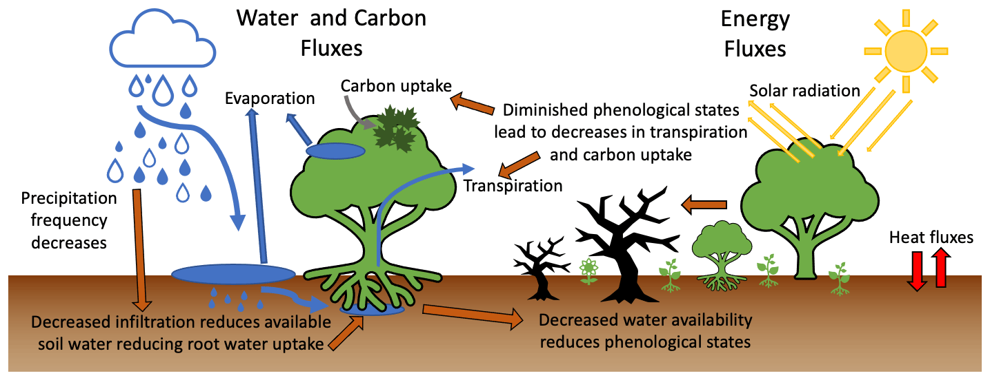
Figure 1 Schematic of water, carbon, and energy fluxes with hypotheses about the ecohydrological response to flash drought indicated with dark orange arrows. A decreased frequency of precipitation events leads to decreased infiltration and less water being available for plant use during flash drought periods compared with non-flash-drought periods. During flash drought, the cascading effects of decreased water availability, exacerbated by the reduced phenological states and stomatal conductance, include rapid reductions in transpiration and atmospheric carbon uptake to levels below other drought periods.

2 Methods and data

2.1 Overview of modeling approach

Remotely sensed or ground observations of land and atmospheric responses to flash drought are useful for identifying changes in plant phenology, soil moisture, and evaporation rates, among others, but observations alone are unable to fully explain the mechanisms driving ecological responses and water use strategies. Physically based models can help fill the gaps in understanding what drives these changes by identifying key processes in the land–atmosphere interactions. For example, decreases in ground-based or satellite-derived GPP do not illuminate what processes caused the change, whereas a process-based model might be able to signal that changes in root water uptake lead to decreased transpiration rates, which ultimately lead to decreased photosynthesis and carbon assimilation.

Within physical models, changes in land surface variables (e.g., soil moisture, root uptake, and evaporation rates) are dependent upon meteorological conditions, either forced or dynamic (Sellers et al., 1997). Water use strategies are dictated by vegetation phenological states (Hu et al., 2008) and stomatal regulation (Novick et al., 2016), and they strongly influence GPP and ET (Beer et al., 2009). Therefore, physical, process-based models are able to adapt to changing meteorological conditions and capture mechanistic changes in vegetation–atmosphere interactions. Our goal is to identify vegetation responses that occur as a result of flash drought and associate those changes with the physical processes represented in a land surface hydrology model.

To identify the physical mechanisms driving plant responses to flash drought intensification, we use two configurations of the physically based Duke Coupled surface–subsurface Hydrology Model (DCHM) with dynamic Vegetation (DCHM-V) and Predictive Vegetation (DCHM-PV). The DCHM-V provides baseline estimates of soil moisture (SM), root uptake (RU), ET, and GPP using forced phenology from the Moderate Resolution Imaging Spectroradiometer (MODIS) FPAR and LAI products. Instead of using forced phenology, the DCHM-PV uses a prognostic vegetation (i.e., phenological) model to predict the vegetation states of FPAR and LAI using parameters that correspond to seasonality (e.g., temperature and photoperiod), water availability (e.g., soil and vapor pressure deficit), and local vegetation characteristics (Lowman and Barros, 2018; Kim et al., 2015; Caldararu et al., 2014; Stöckli et al., 2008; Moradkhani et al., 2005). An ensemble Kalman filter (EnKF) data assimilation procedure following Lowman and Barros (2018) is used to estimate ensembles of parameters for use in the predictive phenology model. Monte Carlo simulations of the DCHM-PV with the ensembles of predictive phenology parameters from the data assimilation step are used to explore the propagation of error and uncertainty. We validate model simulations against ground observations, remotely sensed data, and other modeled products. A summary of the data sets used to force or validate both configurations of the DCHM is provided in Table 1.

Du (2011)Mitchell et al. (2004)Xia et al. (2012)Myneni et al. (2015)Friedl and Sulla-Menashe (2015)Miller and White (1998)Baldocchi et al. (2001)Running et al. (2015)Xia et al. (2012)Tobin et al. (2019)

Table 1 Summary of data products and uses.

2.2 Forcing data sets for DCHM

2.2.1 Meteorological

The 1-D DCHM-V and -PV spatial and temporal resolution is set to the same scale as the highest-quality precipitation forcing data available. For this study, the model uses the native resolution of the Stage-IV precipitation forcing from the National Oceanic and Atmospheric Administration (NOAA) National Centers for Environmental Prediction (NCEP) (Du, 2011). The Stage-IV data set has a 4 km spatial resolution, a 1 h temporal resolution, and a record beginning in 2002. All forcing data sets were interpolated to the Stage-IV resolution for the entire continental US (CONUS) before study-site-specific data were extracted. Atmospheric forcing data (downward shortwave and longwave radiation, air temperature, specific humidity, surface pressure, and wind velocity) used in the DCHM are from Phase 2 of the North America Land Data Assimilation System (NLDAS-2) Forcing File A (Mitchell et al., 2004). NLDAS-2 is a combination of observational and reanalysis data sets intended for use in land surface models like the DCHM. The data are available at a 0.125° spatial resolution and 1 h temporal resolution. They are spatially interpolated to the 4 km Stage-IV grid. No temporal interpolation was necessary.

2.2.2 Land cover

The land surface albedo and fraction of vegetation cover used in the DCHM-V and -PV come from the NLDAS-2 Mosaic Land Surface Model L4 data set at a 0.125° spatial resolution and 1 h temporal resolution (Xia et al., 2012; Mitchell et al., 2004). NASA’s MODIS Land Cover (MCD12Q1) remotely sensed satellite land cover classification product is used to determine land cover type within DCHM. In particular, we use the University of Maryland classification scheme (Sulla-Menashe and Friedl, 2018). Within the model, land cover type is updated yearly. The native spatial resolution of this data set is 500 m, and it is interpolated to the 4 km resolution using a nearest-neighbor approach.

2.2.3 Soil texture and porosity

Soil texture and porosity data were acquired from the Soil Information for Environmental Modeling and Ecosystem Management CONUS-SOIL data set (Miller and White, 1998). The CONUS-SOIL spatial resolution is 1 km with 11 layers. We upscaled the raw soil texture and porosity data to the 4 km Stage-IV grid using two different methods. By averaging over the top 100 cm, we avoid averaging layers interpolated as bedrock (and thus near zero porosity). We approximate soil porosity by averaging the top eight layers (100 cm), and we represent texture using the texture mode across each grid cell and layer.

2.2.4 Vegetation

MODIS LAI and FPAR data were obtained for all of CONUS at the native 500 m spatial and 8 d temporal resolution. Before linearly interpolating the data to the Stage-IV grid and time step, the data for each pixel were smoothed using a Savitzky–Golay filter (Savitzky and Golay, 1964), following the algorithm presented in Chen et al. (2004), in order to preserve seasonality and reduce noise in the data from cloud contamination and other atmospheric disturbances that may alter surface reflectance observations (Cihlar et al., 1997; Tanré et al., 1997). We use an m=6 scaling window and d=4° for the interpolating polynomial (Chen et al., 2004; Lowman and Barros, 2016).

2.3 Data sets used for model comparison

We assess vegetation responses to the Kansas flash drought of 2012 by comparing model results of land surface, subsurface, and atmospheric carbon and water fluxes (e.g., SM, GPP, and ET) to multiple ground and remotely sensed observations. Modeled SM fluxes from the DCHM-V and -PV are compared to SoilMERGE (SMERGE), NLDAS-2 Noah model output, and AmeriFlux eddy covariance. SMERGE is a 0.125° root-zone (0–40 cm) SM product obtained from “merging” NLDAS-2 outputs with European Space Agency Climate Change Initiative surface satellite data that can predict vegetation health anomalies (Tobin et al., 2019). Because SMERGE only provides root-zone SM, we only compare it to the DCHM middle-layer SM output. We also validate SM estimates against NLDAS-2 estimates from the Noah land surface model (LSM) for all three soil layers used in DCHM Xia et al., 2012). When AmeriFlux SM data are available, we compare them with modeled soil moisture from the top layer, as most AmeriFlux SM sensors are in the top few centimeters of soil. The DCHM-V and -PV estimates of GPP are compared to the MODIS (MOD17A2H) GPP product and AmeriFlux eddy covariance outputs of GPP. We also compare DCHM estimates of ET to AmeriFlux eddy covariance flux tower estimates by dividing the observed latent heat flux by the latent heat of vaporization of water (λ_w=2.5 MJ kg⁻¹; Dingman, 2015).

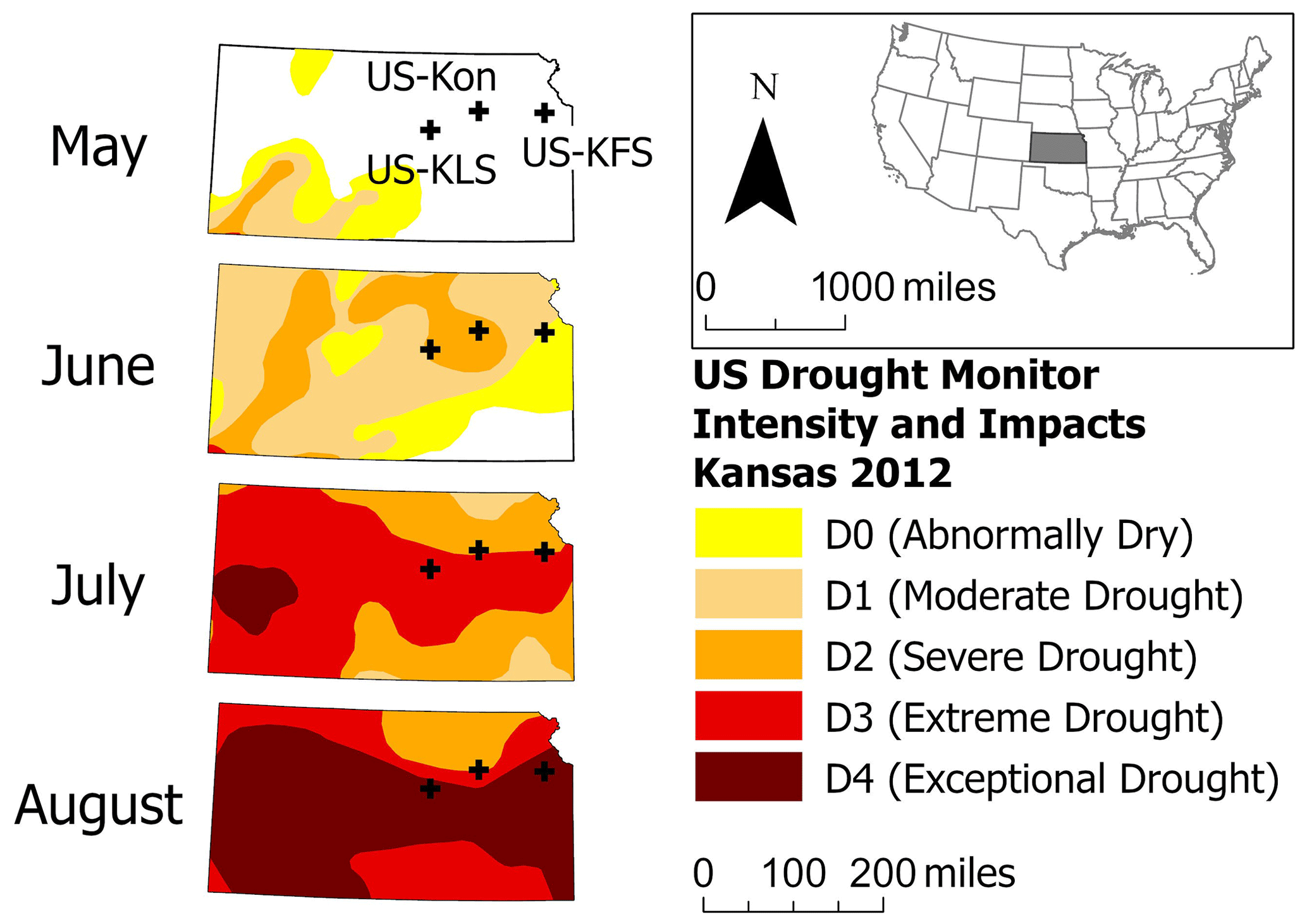
Figure 2 Evolution of the 2012 flash drought from May to August in the U.S. Drought Monitor with the three AmeriFlux tower study sites (US-KFS, US-KLS, and US-Kon). Note that 1 mi is equivalent to approximately 1.61 km.

2.4 Description of study sites

This study focuses on three AmeriFlux sites in Kansas (US-KFS, US-KLS, and US-Kon; Fig. 2, Table 2), chosen because of the availability of GPP and latent heat (converted to ET) data during the flash drought year of 2012 and at least 1 wet year after 2012. When available, we used gap-filled FLUXNET FULLSET data for US-KFS and US-Kon (Pastorello et al., 2020). All three sites are classified as grasslands according to the International Geosphere–Biosphere Programme (IGBP) land cover, and all three sites have Cfa (humid, subtropical) Köppen climate classifications (Brunsell, 2020a, b, 2021). US-KFS is located within a grassland–deciduous forest boundary area and receives 1014 mm of precipitation annually (Brunsell, 2020a). US-KLS is a perennial agricultural study site receiving 812 mm of rainfall each year (Brunsell, 2021). US-Kon is part of the Konza Prairie Long-term Ecological Research (LTER) program, receives 867 mm of precipitation, and is burned annually. Static characteristics of PFT, soil texture and porosity, and geographic information for the study sites are shown in Table 2. According to the MODIS Land Cover Type classification product (MCD12Q1), each site had a unique vegetation cover type (savanna, grassland, and cropland; Table 2). The PFT is a result of interpolating MODIS MCD12Q1 Land Cover Type 2 to the 4 km grid and does not align with the land cover from AmeriFlux in all cases. The soil texture and porosity are interpolated CONUS-SOIL (Miller and White, 1998) values.

Brunsell (2020a)Brunsell (2021)Brunsell (2020b)

Table 2 AmeriFlux study sites contained within Stage-IV pixels.

Plant functional type (PFT), soil texture, and soil porosity were determined after interpolation to the Stage-IV grid. The abbreviations used in the table are as follows: SAV – savanna; CRO – cropland; GRA – grassland. Precipitation totals are listed as the AmeriFlux annual mean.

2.5 Description of modeling work

2.5.1 Land surface hydrology model

We employ two 1-D versions of the DCHM coupled land surface hydrology model that accounts for water and energy exchanges between three soil layers, the surface, and the atmosphere (Lowman and Barros, 2018, 2016; Tao and Barros, 2014, 2013; Yildiz and Barros, 2009, 2007, 2005; Gebremichael and Barros, 2006; Garcia-Quijano and Barros, 2005; Devonec and Barros, 2002; Barros, 1995). A 4 km grid resolution and 1 h time step were chosen to run the model to match the native spatial resolution of the Stage-IV precipitation data, as precipitation is the main source of uncertainty when modeling drought (Trenberth et al., 2014). We use 80 mm for the top-layer soil depth to ensure model stability, but the middle and deep layers were selected to best match the USDA Kansas soil profile (Soil Survey Staff, 2022). This yields three soil layers: top (0–80 mm), middle (80–890 mm), and bottom (890–1830 mm). Rooting depth and density, which are used to determine the total root water uptake in the DCHM, are calculated using empirical exponential root distribution functions that vary by PFT (Lowman and Barros, 2016; Zeng, 2001; Lai and Katul, 2000; Jackson et al., 1996; Clausnitzer and Hopmans, 1994). Soil layer and rooting depths align with the different combinations of soil textures and PFTs found in Thornthwaite and Mather (1957).

The DCHM water balance includes subroutines for evaporation from the different components of the land surface (i.e., bare soil and vegetation), ponding and groundwater runoff, snow accumulation and melt, and root water uptake, while energy balance routines solve for net radiation as well as sensible, latent heat, and ground heat fluxes (Lowman and Barros, 2018, 2016; Tao and Barros, 2014, 2013; Yildiz and Barros, 2007, 2005; Garcia-Quijano and Barros, 2005; Devonec and Barros, 2002; Barros, 1995). The water and energy balances both influence photosynthesis, which is simulated using the Farquhar model (Lowman and Barros, 2016; Garcia-Quijano and Barros, 2005; Farquhar and Caemmerer, 1982; Farquhar et al., 1980).

2.5.2 Predictive phenology

The key difference between the two versions of the DCHM used for this study is that vegetative phenology is forced using the MODIS MOD15A2H FPAR and LAI products within the DCHM-V, whereas the DCHM-PV predicts phenology for the next day based on the current-day conditions. Establishing differences in the outputs from the DCHM-V and -PV illuminates changes in plant growth strategies. MODIS is a passive sensor and uses only the red (648 nm) and near-infrared (NIR, 858 nm) spectral bands to estimate LAI values (Myneni et al., 2015). Within the DCHM-PV, the Dynamic Canopy Biophysical Properties (DCBP) model predicts plant life stage based on climatological properties of water availability, air temperature, and evaporative demand (Lowman and Barros, 2018). FPAR and LAI are dynamically estimated instead of forced using MODIS observations to evaluate impacts on estimates of ET and GPP (Lowman and Barros, 2018; Kim et al., 2015; Caldararu et al., 2014).

The DCBP is the predictive phenology model that determines future plant growth based on differences between current and potential phenological states. The growing season index (GSI) determines potential phenological state based on current climate conditions (Jolly et al., 2005; Stöckli et al., 2008). Specifically, it is a function of temperature, photoperiod, soil water potential, and vapor pressure deficit (VPD; Lowman et al., 2023; Lowman and Barros, 2018). Lowman and Barros (2018) adapted the framework to incorporate soil water parameters that affect predictions of plant growth stage. The DCBP is implemented within the DCHM-PV to estimate phenologic state with the land surface hydrology model. However, to do this, we must first estimate parameters that determine plant growth rates and sensitivity to meteorological and soil conditions.

A Bayesian hierarchical approach is used to estimate the parameters for the DCBP. Specifically, a dual state–parameter ensemble Kalman filter (EnKF) is used to jointly estimate the phenologic states of FPAR and LAI as well as the 11 other parameters within the DCBP (Table 3; Lowman et al., 2023; Lowman and Barros, 2018). This method was described by Moradkhani et al. (2005) as a way of simultaneously predicting states and parameters in hydrologic models; it was then later implemented by Stöckli et al. (2008) to assimilate remotely sensed observations of LAI and FPAR into a predictive phenology model.

Table 3 Ensemble mean and 1 standard deviation (SD) of predictive phenology model parameters from the 3YR assimilation period.

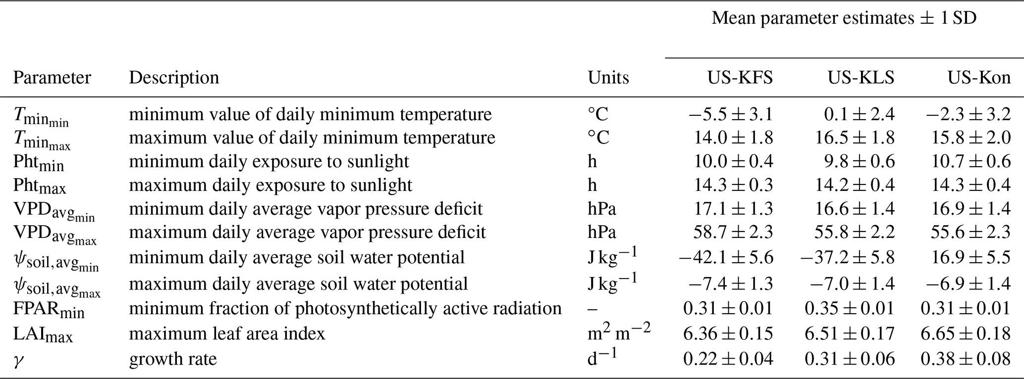
For an in-depth description of the predictive phenology routine within dynamic the Canopy Biophysical Properties (DCBP) model, the reader is referred to Lowman et al. (2023) and Lowman and Barros (2018).

The parameter estimation procedure first consists of creating a prior distribution by sampling each state and parameter from a Gaussian distribution. This generates N=2000 ensemble members. Phenological states and input parameters are updated at every time step for the duration of the data assimilation period using the EnKF. We assimilate MODIS LAI and FPAR every 8 d (the native MODIS temporal resolution) to reduce error and ensure that phenological state predictions do not stray too far from observations (Lowman et al., 2023; Lowman and Barros, 2018).

2.6 Model simulations

We run both the DCHM-V and -PV from 2002 to 2019 at a 1 h time step and 4 km spatial resolution, spinning up 2002 three times to allow for model stabilization (Lowman and Barros, 2016, 2018). The DCHM-V simulations provide a baseline for changes in water, energy, and carbon exchange using forced phenology from MODIS, whereas the DCHM-PV simulations implement a predictive phenology scheme, allowing us to investigate how dynamic changes in the plant growth strategy impact the aforementioned fluxes.

In order to run the DCHM-PV, we first generate phenology model parameters for the predictive phenology routine. Specifically, we use 2003 (DRY), 2005 (WET), and 2003–2005 (3YR) as the data assimilation periods in the DCBP model to generate parameters that correspond to dry, wet, or average precipitation regimes, respectively (Table 4). We use three different assimilation periods in order to capture the sensitivity of phenology model parameters to the meteorological conditions. It has been shown, under varied climatological conditions, that plants can be highly adaptable, transitioning from isohydric to anisohydric in a single season (Guo et al., 2020). Lowman and Barros (2018) showed that the assimilation period can determine the water stress adaptations for the modeled vegetation state. Broadly speaking, vegetation model parameters predicted using data from years with minimal rainfall represent plants accustomed to drier conditions; therefore, plants would exhibit more regulation in their water use tendencies (Lowman and Barros, 2018; Sade et al., 2012).

Table 4 Summary of precipitation conditions during data assimilation periods.

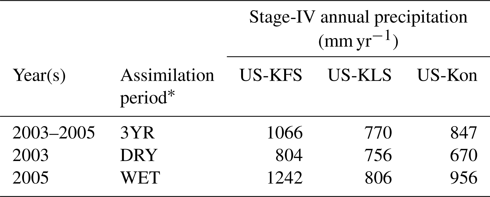
^* The data assimilation periods are as follows: 3YR represents a period with average annual precipitation; WET and DRY are periods with above- and below-average annual precipitation, respectively.

To incorporate uncertainty from the phenology parameter estimation step into the DCHM-PV simulation, we run the model as Monte Carlo simulations with N=2000 members. Each ensemble member is sampled from a Gaussian distribution using the final mean and standard deviation of the parameter estimates from each of the assimilation periods. In our results, we focus on analyzing model output from 2006 to 2019 in order to omit the 2003–2005 period used in the data assimilation step from our analysis.

2.7 Analysis of model outputs

In this paper, we are interested in exploring whether land surface, subsurface, and atmospheric interactions are distinct during flash drought periods compared with drought and non-drought periods. We focus on results from the three AmeriFlux sites for 2012 (flash drought), 2018 (drought), and 2019 (non-drought) to draw conclusions about plant response during flash drought and how they differ from drought and non-drought years. We evaluate model outputs from 2006 to 2019 to assess the differences between the DCHM-V and DCHM-PV model configurations during drought and non-drought years compared with a flash drought year. During this time period, we identified drought years as 2006, 2011, 2013, 2014, and 2018 and non-drought years as 2007–2010, 2015–2017, and 2019 using the USDM for the central and east-central Kansas climate regions (Svoboda et al., 2002). Drought years were determined by whether parts of the region reached the D2 “Severe Drought” classification or higher. When computing drought and non-drought averages, we use the years listed here. In many time series results, we display the water year (April–October) rather than the entire year, as plants are largely dormant outside of the water year in a temperate region (Dai et al., 2016; Wang et al., 2003; Towne and Owensby, 1984). Transpiration is calculated from total root water uptake through the three soil layers, and total evaporation is computed by summing evaporation from ground and canopy surfaces, allowing us to partition ET into evaporation and transpiration (Lowman and Barros, 2018; Lai and Katul, 2000). Water use efficiency is represented as the ratio of GPP and ET (WUE = GPP / ET; Beer et al., 2009). We highlight differences between the DCHM-V and DCHM-PV model simulations and compare outputs to remotely sensed and in situ observations where available.

3 Results

3.1 Phenology

3.1.1 Growth rate parameter

The growth rate parameter, γ, dictates how much the phenological state (i.e., FPAR and LAI) can change in a given time step (Lowman and Barros, 2018; Stöckli et al., 2008). The uncertainty in γ shows the variability in vegetation responses to changing phenological states. Lower uncertainty in γ establishes the 3YR assimilation period, with a mixture of wet and dry years, as the preferred choice for running the DCHM-PV (Fig. 4). This finding is in agreement with Lowman and Barros (2018), who found that using assimilation periods with both wet and dry conditions has the effect of capturing adaptive plant water use strategies. This lower uncertainty propagates through the DCBP in DCHM-PV, leading to lower uncertainty in the predictions of FPAR and LAI (Figs. 5, 6). The values of γ vary by site due to a combination of local climate and vegetation type. US-KFS, modeled as a savanna, has the lowest mean and standard deviation of γ (Table 3). The smaller magnitudes of the growth parameters indicate that vegetation is less likely to make abrupt changes and exhibit more resilience when faced with extreme dry down. Other parameter estimation outputs used to generate ensembles from the 3YR assimilation period can be found in Table 3.

Figure 3 Schematic of the modeling workflow. Spatial and temporal resolutions of all forcing data are interpolated to match the resolution of the Stage-IV precipitation (4 km and 1 h), which is the resolution used for DCHM in this study. Land cover, soil properties, and atmospheric forcing inputs come from MODIS, STATSGO (CONUS-SOIL), and NLDAS-2, respectively. Simulations were run from 2002 to 2019. We generated ensembles of parameters for three different precipitation regimes: 2003 (DRY), 2005 (WET), and 2003–2005 (3YR) for the predictive phenology routine in the DCHM-PV. The data assimilation procedure used an ensemble Kalman filter (EnKF) with simulated soil water potential and vapor pressure deficit from the DCHM-V, MODIS MOD15A2H FPAR/LAI, and concurrent meteorological conditions. The DCHM-V outputs of interest included evapotranspiration (ET), root water uptake (RU), and gross primary productivity (GPP). Additional DCHM-PV outputs included the predicted fraction of photosynthetically active radiation (FPAR) and leaf area index (LAI).

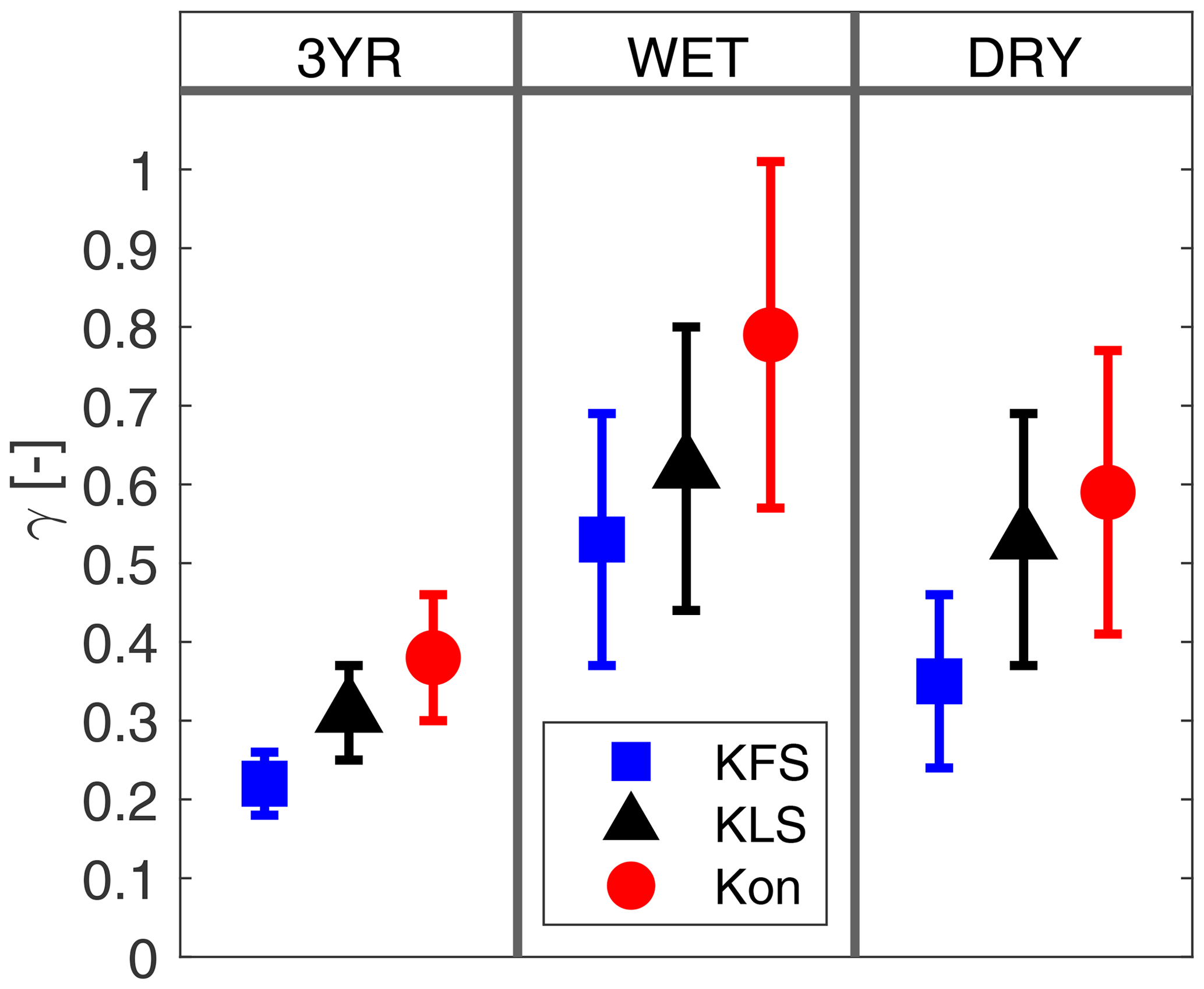
Figure 4 Ensemble means and 1 standard deviation of the growth rate parameter, γ (–), for each site and all three data assimilation periods: 3YR (2003–2005), WET (2005), and DRY (2003).

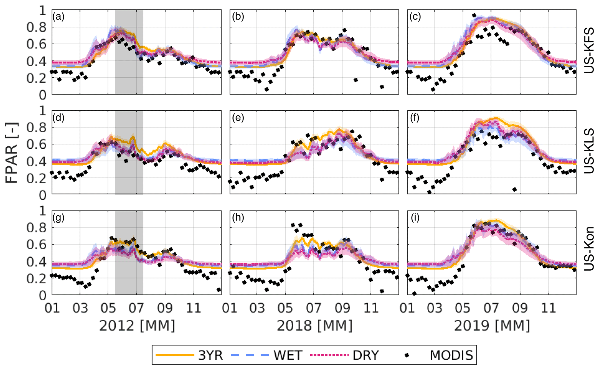
Figure 5 Fraction of photosynthetically active radiation, FPAR (–), predicted from the DCHM-PV for a flash drought year (2012), drought year (2018), and non-drought year (2019) for US-KFS (a–c), US-KLS (d–f), and US-Kon (g–i). Colors indicate the different data assimilation periods: 3YR (yellow), WET (blue), and DRY (red). Corresponding shaded regions represent 1 standard deviation of model outputs from the 2000 ensemble members. The 8 d MODIS MOD15A2H FPAR is shown as black dots. The gray shaded regions in panels (a), (d), and (g) highlight the 2012 flash drought period.

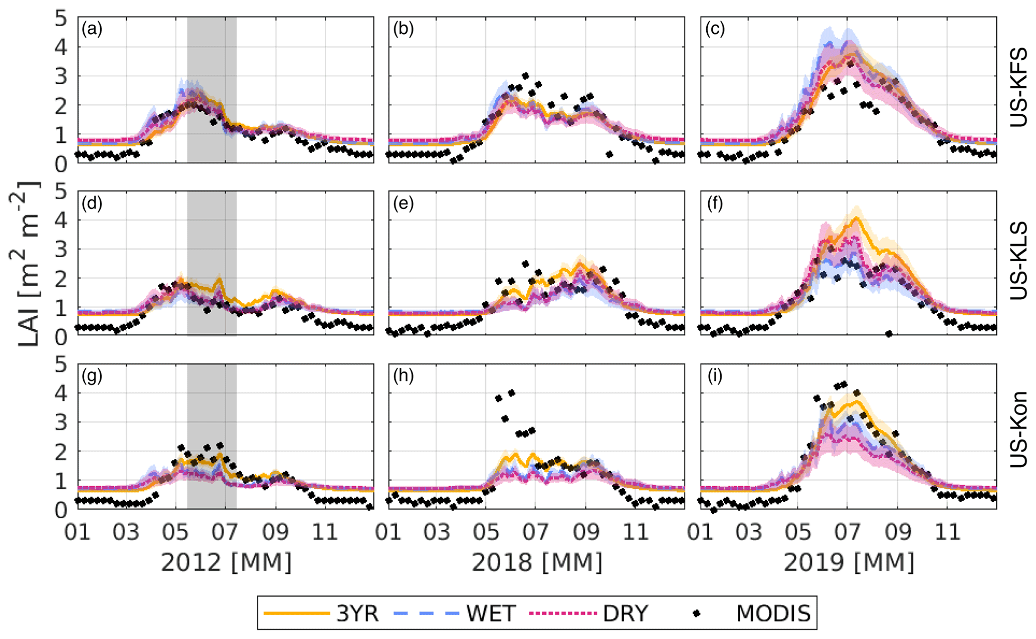
Figure 6 Leaf area index, LAI (m² m⁻²), predicted from the DCHM-PV for a flash drought year (2012), drought year (2018), and non-drought year (2019) for US-KFS (a–c), US-KLS (d–f), and US-Kon (g–i). Colors indicate the different data assimilation periods: 3YR (yellow), WET (blue), and DRY (red). Corresponding shaded regions represent 1 standard deviation of model outputs from the 2000 ensemble members. The 8 d MODIS MOD15A2H LAI is shown as black dots. The gray shaded regions in panels (a), (d), and (g) highlight the 2012 flash drought period.

3.1.2 Fraction of photosynthetically active radiation

Overall, the DCHM-PV-simulated FPAR tends to follow the same patterns as MODIS throughout the growing season, irrespective of the choice of parameters. Results indicate slower senescence and reduced variance using the 3YR assimilation parameters compared with the WET and DRY parameters during late June and early July 2012 across all three sites (Fig. 5a, d, g). This aligns with the known period of flash drought that occurred across Kansas (Lisonbee et al., 2021). The predicted values of FPAR at US-KFS and US-KLS are slightly higher than the MODIS values during the 2012 growing season. The predicted values of FPAR match well against MODIS for the US-Kon site, especially during the decline in late-June through July. During the flash drought period, there is a notable decrease in variance, or uncertainty, across the Monte Carlo simulations.

For US-KFS, across the three simulations, the simulation using the WET parameters achieves a higher FPAR during the flash drought and holds its peak throughout the month of May, with declines beginning in June and bottoming in early July before rising again in the latter part of the growing season. FPAR decreases from 0.77 to 0.41 for the WET parameters, while reductions from the time of peak FPAR to early July in the simulations using DRY and 3YR parameters are from 0.73 to 0.47 and from 0.76 to 0.53, respectively. The decreases in FPAR observed from mid-May to mid-July in 2012 are more pronounced than during the growing season of the drought year 2018 (when fluctuations in FPAR were smaller). Results from an above-average precipitation year (2019) show a steady increase, a longer peak growing season, and a decrease in line with fall senescence across all simulations. However, using WET and DRY parameters at US-KLS led to a ∼ 0.2 reduction in FPAR in July 2019, opposed to a ∼ 0.1 reduction from the 3YR parameters. The larger decrease is likely due to the below-average July precipitation and the larger WET and DRY values of γ leading to faster phenological changes. Similarly to the 2012 results, 2019 simulations using phenology parameters from the 3YR assimilation period showed slower late-season declines in FPAR than simulations using parameters from the WET or DRY assimilation periods. This can be seen from the 3YR parameter simulations for US-KLS and US-Kon, which show higher FPAR through July.

3.1.3 Leaf area index

Predicted values of LAI are similar to MODIS LAI with small relative differences (Fig. 6). During the flash drought year of 2012, a steep decline in modeled LAI can be seen in late June and early July across the three sites. LAI declines almost 1 m² m⁻² in a few weeks during summer 2012 compared with steadier values during the drought of 2018. Growing season LAI was ∼ 0.5 m² m⁻² lower in 2012 compared with 2018. The DCHM-PV model outputs of LAI during 2019 match MODIS but are 1–2 m² m⁻² higher during June, July, and early August at US-KFS and US-KLS, and slightly lower than MODIS at US-Kon.

Simulated LAI values vary slightly across the three sites. For US-KFS, simulations using the WET year parameters achieve higher LAI values than the other two simulations (Fig. 6a, b, c). For US-KLS and US-Kon, the growing season LAI has the highest peaks in the simulations using the 3YR parameters (Fig. 6d, e, f, g, h, i). With more rainfall in May and June 2019, the simulations using the WET parameters result in a lower LAI than the simulations using the DRY parameters.

The most consistent similarities across the phenology results is that the simulations using the 3YR parameters generally show a slower decline in LAI in flash drought and non-flash-drought years for all sites. Additionally, the simulations using WET and DRY parameters are more similar to each other than to the simulations using 3YR parameters. This result is commensurate with the values of the means and variances of γ resulting from the different assimilation periods. Simulations using the 3YR assimilation period result in the LAI remaining high for a longer period of time with a decrease in response to flash drought developing more slowly than for the other two simulations. This is also apparent for US-KLS and US-Kon in the 2019 3YR simulations in which leaf growth continues through June and peaks in the middle of July, whereas new growth tends to slow from the beginning of June through mid-July in the WET and DRY simulations.

Generally, the predictive phenology model compares favorably with the seasonal changes observed in MODIS FPAR and LAI (Figs. 5, 6) in both flash drought and non-flash-drought periods. In the summer, at US-KFS and US-KLS during 2019, the model tends to predict FPAR and LAI values higher than MODIS. In 2019, at US-KFS, MODIS observed a steady decline in FPAR from 0.8 to 0.6 throughout July followed by an increase to 0.8 over an 8 d period at the beginning of August (Fig. 5c). The DCHM-PV results do not show the same decline. Similarly, MODIS observes a drop in LAI before an abrupt increase, while model estimates remain higher than MODIS (Fig. 6c). However, in June 2019, the DCHM-PV estimates at US-Kon are lower than MODIS LAI.

The bulk of the following results and analysis compares vegetation responses during flash drought and non-flash-drought periods, rather than an inter-model comparison across the different assimilation strategies. Estimates from the WET and DRY simulations tend to be in agreement with results from the 3YR simulations. From this point forward, we only show results from the 3YR simulations.

3.2 Subsurface water

3.2.1 Infiltration

During non-drought years, monthly infiltration accumulation amounts are above or near 100 mm per month, on average, from April to July, with the highest amounts in May (Fig. 7). During drought years, infiltration between April and July is less than non-drought years. Furthermore, monthly accumulated infiltration is lower during the flash drought year compared with both drought and non-drought years, suggesting that there is less water available for plant use during the growing season. At US-KFS from April to October of 2012, monthly infiltration is slightly below what is observed during drought years. A large decline in May infiltration at US-KLS and US-Kon led to infiltration accumulation amounts that were 1–2 standard deviations below average drought conditions. All sites had infiltration rates below 100 mm for all months during 2012 with the exception of US-KLS in August 2012.

Figure 7 The DCHM-PV 3YR ensemble means of monthly infiltration accumulation amounts (mm) for drought (red) and non-drought (blue) years compared to 2012 (black) for US-KFS (a), US-KLS (b), and US-Kon (c). Monthly sums are computed from the ensemble means of the 2000 Monte Carlo simulations and then averaged across drought or non-drought years. Error bars represent 1 standard deviation across drought and non-drought years.

Low monthly infiltration amounts during the flash drought year are likely due to lower precipitation accumulation, coupled with an increase in the number of days between precipitation events, and an increase in atmospheric demand for water (Fig. 8 and Figs. S4 and S5 in the Supplement). During drought and non-drought years, the average number of days between rainfall events within a month ranges from 1 to 7 d, while the lower end for the flash drought year is higher (2.5 d). Here, we consider a rainfall event to be any day with recorded precipitation. Additionally, during drought and non-drought years, monthly infiltration exceeds 150 mm; however, it remains at or below 75 mm for all sites in 2012 aside from August 2012 at US-KLS, where monthly infiltration is ∼ 110 mm. In 2012, all three sites averaged over 4 d between rainfall events during May, June, and July, with US-KFS averaging over 6 d between rainfall events during both May and June and more than 5 d in July (Fig. 8a). Across all three sites from April to October 2012, there was more than 4 d between precipitation events 80 % of the time compared with just 20 % of the time in non-flash-drought years.

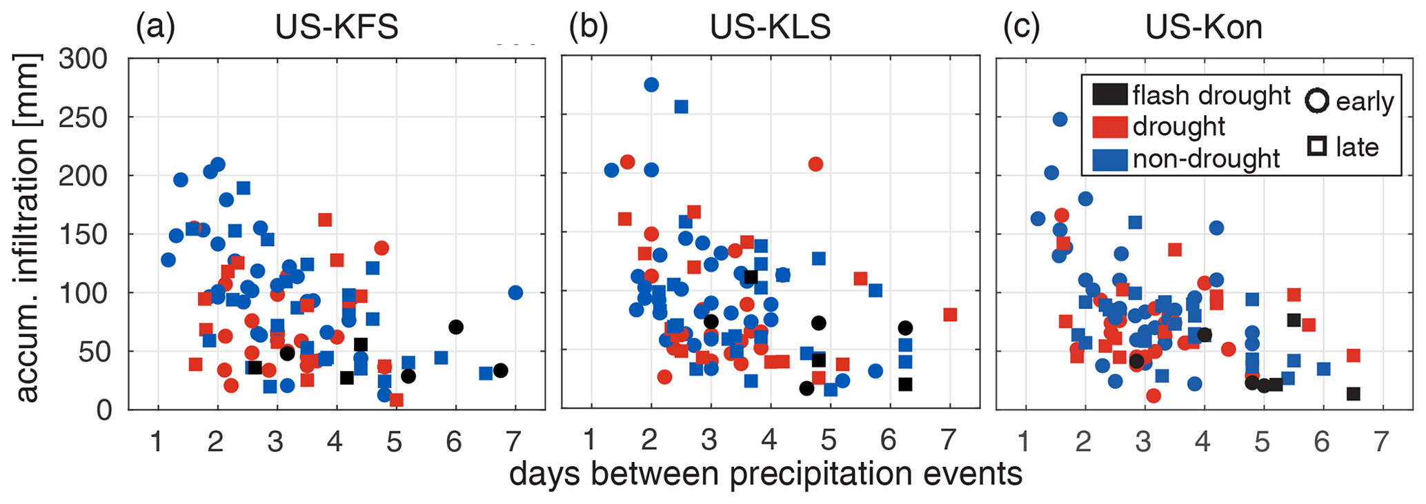
Figure 8 Monthly infiltration accumulation (mm) vs. average days between precipitation events within a single month for (a) US-KFS, (b) US-KLS, and (c) US-Kon. Each shape indicates whether the month occurs in the early growing season (circles: April–July) or late growing season (squares: August–October). Colors distinguish flash drought years (black) from drought years (red) and non-drought years (blue).

3.2.2 Soil moisture

Soil moisture analysis and comparison to other soil moisture products are similar for all three study sites. Figures for soil moisture at US-KFS for all three soil layers are available in the Supplement. Top-layer soil moisture reaches the wilting point several times throughout the flash drought period of 2012 (Fig. S1a). During peak flash drought, at the end of June and beginning of July, the moisture content remains at wilting point for many days. Daily soil moisture agrees with AmeriFlux soil moisture observations in the top layer during 2012 at US-KFS. Discrepancies exist in 2018, when AmeriFlux observations fall to levels just above 0 m³ m⁻³.

Fluctuations in soil moisture match favorably with NLDAS-2 estimates across the top two layers in 2012, 2018, and 2019. However, middle-layer soil moisture from the DCHM estimates is about 0.05 m³ m⁻³ higher than NLDAS-2 and SMERGE by the late growing season of the flash drought year (Fig. S2). The DCHM estimates remain fairly steady in the deep layer during 2012, while NLDAS-2 soil moisture estimates continue to fall throughout the rest of the growing season (Fig. S3). The steady DCHM soil moisture levels during flash drought may be indicative of the modeling stunting root water uptake during the same time, thereby preserving soil water content.

3.2.3 Root water uptake

Root water uptake is above non-flash-drought levels in 2012 before the onset of flash drought in June. It then remains lower than non-flash-drought levels for the remainder of the growing season (Fig. S6). The middle soil layer is responsible for up to 4 times more root water uptake than the other layers. Thus, a major decline in root water uptake through the middle layer is informative of how plant water use is altered during drought. While root water uptake starts out at levels above average non-drought years in 2012, it falls to more than 1 standard deviation below drought averages by July. This drastic shift is likely due to lower infiltration (Fig. 7), and it drives down rates of transpiration within the DCHM-V and -PV over the same period.

3.3 Plant–atmosphere interactions

3.3.1 Sub-daily stomatal conductance

Sub-daily estimates of stomatal conductance highlight how VPD can drive stomatal activity within DCHM. In 2012, stomatal conductance in the first week of May was as high or higher than in 2019, a non-drought year at US-KFS (Fig. 9). However, by July, major differences in 2012 and 2019 stomatal conductance coincide with changes in VPD. In July 2012, high VPD shuts down midday stomatal conductance, whereas lower VPD values allow for higher rates of stomatal conductance during the same time in 2019. The large decrease in stomatal conductance from the first week of May to the first week of July during the flash drought year of 2012 is unlike that seen in a drought year like 2018, when stomatal conductance rates are similar in May and July.

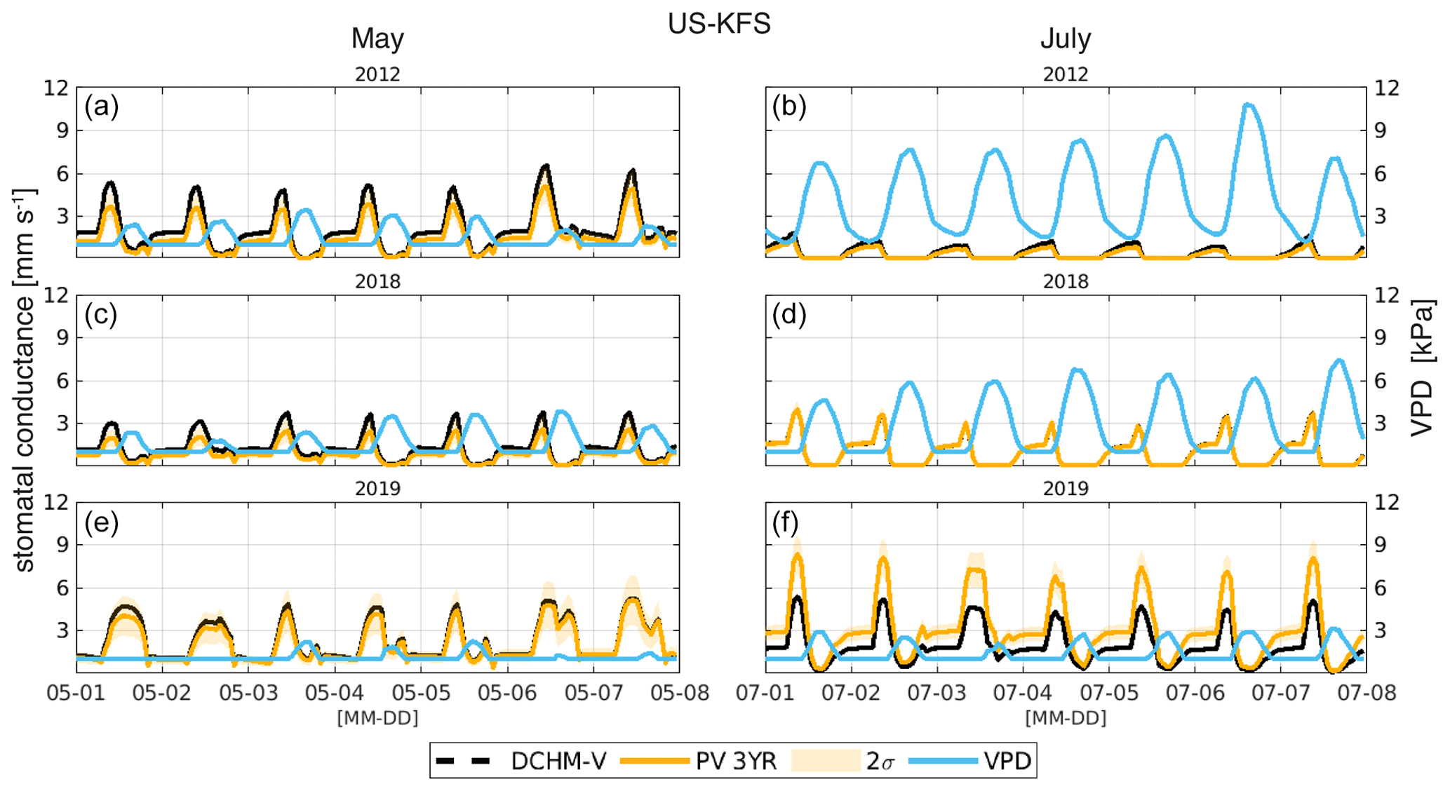
Figure 9 Stomatal conductance (mm s⁻¹) and VPD (kPa) for 1 week in May (a, c, e) and July (b, d, f) of 2012, 2018, and 2019 for US-KFS.

3.3.2 Gross primary productivity

Monthly averages of GPP accumulation from the DCHM-PV ensemble means throughout the water year (April–October) indicate that carbon uptake falls below drought averages from May to June during the flash drought year of 2012 (Fig. 10a, c, e). Flash drought carbon assimilation amounts remain below drought levels before converging to average drought/non-drought levels by the end of October. GPP amounts are up to 50 % lower in drought years compared with non-drought years. During the flash drought, GPP monthly totals in June through August 2012 are at least 1 standard deviation lower than drought years averaged over the 2006–2019 simulation period. June 2012 GPP accumulation values are half of those for drought years and less than 30 % of those for non-drought years. An even greater discrepancy is apparent in July, with carbon assimilation amounts less than 30 % of drought levels and 15 % of non-drought levels. Despite increased GPP from July to August in 2012, values are still 1 standard deviation below drought levels.

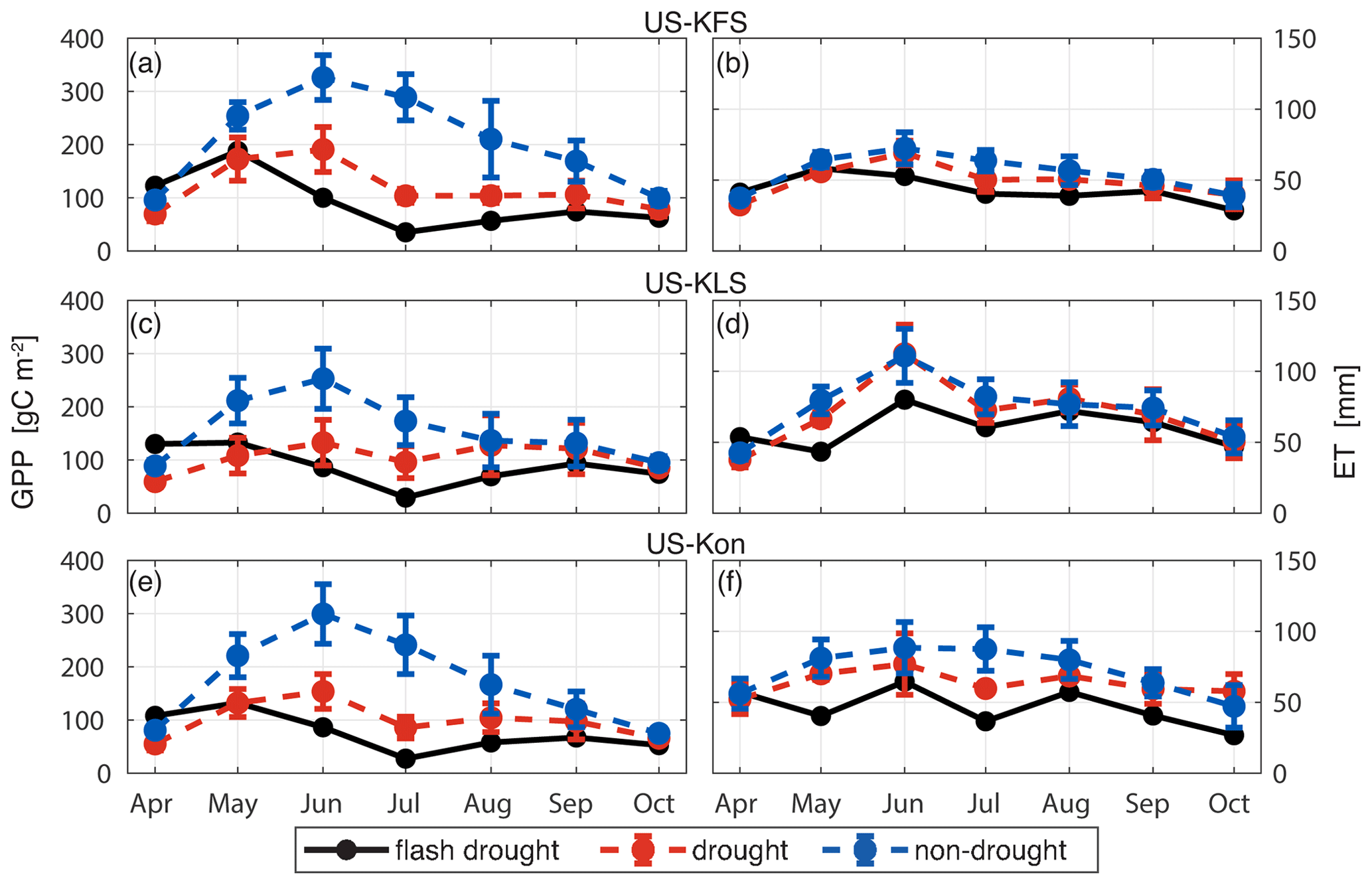
Figure 10 The DCHM-PV 3YR monthly totals of GPP (gC m⁻²) (a, c, e) and ET (mm) (b, d, f) for drought (red) and non-drought (blue) years compared to flash drought (black) for US-KFS (a–b), US-KLS (c–d), and US-Kon (e–f). Monthly totals are computed from the ensemble means of the 2000 Monte Carlo simulations then averaged across drought or non-drought years. Error bars represent 1 standard deviation across drought and non-drought years, respectively.

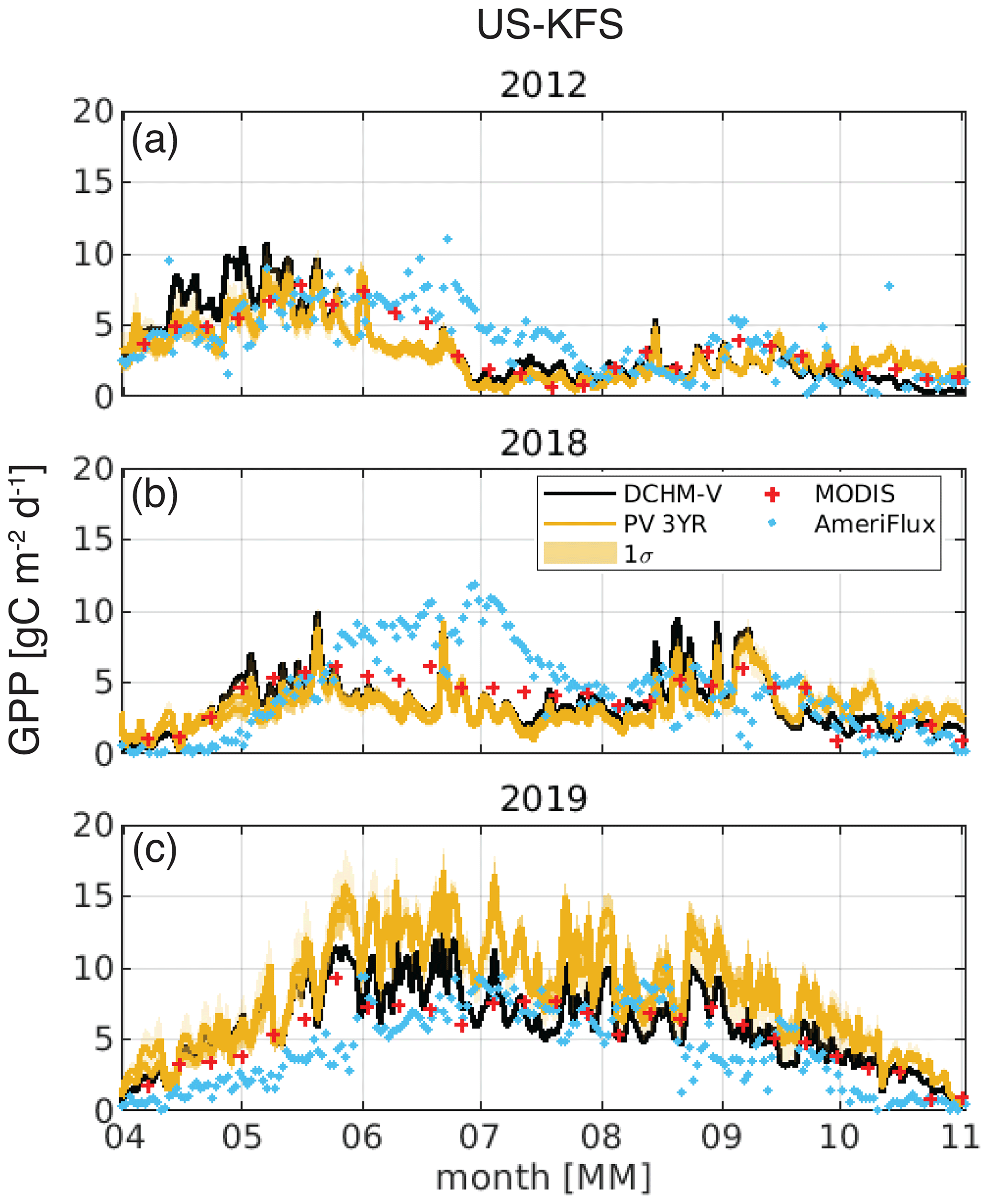
Figure 11 Daily gross primary productivity, GPP (gC m⁻²), at US-KFS for a (a) flash drought year (2012), (b) drought year (2018), and (c) non-drought year (2019). The shaded region for the DCHM-PV simulations denotes 1 standard deviation. MODIS GPP is shown as red crosses and AmeriFlux GPP as blue dots.

Seasonal variations in GPP at US-KFS for simulations from the DCHM-V and -PV (3YR) with observations from MODIS and AmeriFlux for a flash drought year (2012), drought year (2018), and non-drought year (2019) can also be explored at the daily scale (Fig. 11). Daily GPP is lower in drought vs. non-drought years between April and October. During the flash drought year, there is a decline in GPP from 10 gC m² d⁻¹ in early May, above what was observed in 2018 and 2019, to near zero by July in 2012 (Figs. 11, S15 and S16). During the drought year (2018), daily GPP remains low throughout the growing season, but it never decreases to below 1.2 gC m² d⁻¹ at US-KFS. From June to July in 2012, carbon uptake decreased from more than 5 gC m⁻² d⁻¹ to less than 1 gC m⁻² d⁻¹. This type of decline is not observed in a drought year (e.g., 2018). The rapid decline in GPP from May to July is what distinguishes the 2012 flash drought as a period of time during which land–atmosphere interactions switch from resembling conditions that are wetter than an average wet year to drier than an average dry year. The DCHM-PV GPP results are similar to MODIS GPP in most cases, with the exception that they tend to underestimate GPP compared with MODIS in a drought year, aligning with the higher MODIS estimates of FPAR and LAI during the same periods (Fig. 6). Simulated GPP tends to underestimate flux tower GPP during June and July in 2012 and 2018 but overestimates it in 2019.

3.3.3 Stomatal and non-stomatal regulation of gross primary productivity

We examine how GPP covaries during flash drought, drought, and non-drought years with sub-seasonal changes in LAI and stomatal conductance at US-KFS (Fig. 12). During a non-drought year (2019), a wider range of values of stomatal conductance, LAI, and GPP exists throughout the growing season (Fig. 12c). There is a clear seasonal cycle in the clockwise movement through the stomatal conductance–LAI parameter space. Stomatal conductance increases faster than LAI in the early season before reaching maximum values around June. After LAI peaks, there is first a reduction in stomatal conductance and GPP at higher LAI before LAI decreases through August and September.

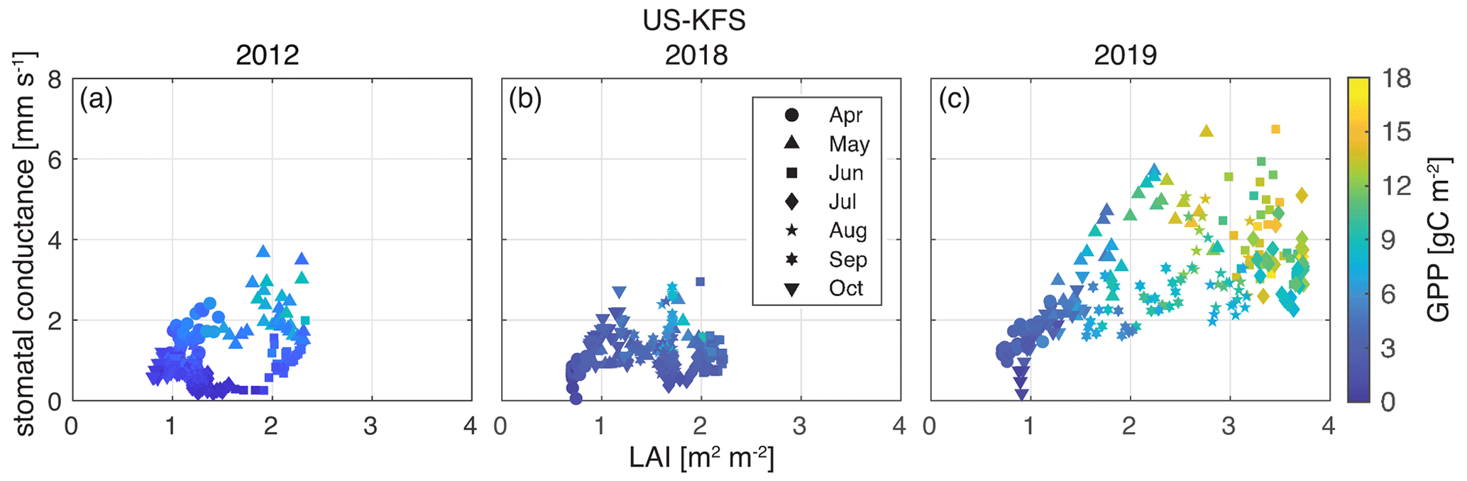
Figure 12 Stomatal conductance (mm s⁻¹) vs. LAI (m² m⁻²) at US-KFS for a (a) flash drought year (2012), (b) drought year (2018), and (c) non-drought year (2019). Marker shapes indicate individual days between 1 April and 31 October. Each month is given a unique shape, the color of which reflects daily GPP values (gC m⁻²).

In contrast, during flash drought (2012) and drought (2018), peak stomatal conductance, LAI, and GPP values at US-KFS are approximately half of 2019 values. Both stomatal conductance and LAI remain low throughout the growing season and GPP is below 10 gC m⁻² at all sites in 2012 (Fig. S7). Stomatal conductance and LAI are highest in May 2012, as opposed to June and July 2019. While both 2012 and 2018 have low values of stomatal conductance, LAI, and GPP, an important difference is the near-zero stomatal conductance during June and July 2012 for a range of LAI values (1–2 m² m⁻²; Fig. 12) that is not observed in 2018 and other drought years (Fig. S11).

The relationship between stomatal conductance, LAI, and GPP is similar across all three sites when considering flash drought (Fig. S7), drought (Fig. S11), or non-drought periods (Figs. S8, S9, and S10). The observable clockwise movement through parameter space is not as clear in flash drought and drought periods compared with non-drought periods. In drought years, stomatal conductance from April to October averages 1.4 mm s⁻¹ across all sites (Fig. S11), compared with 2.3 mm s⁻¹ in non-drought years (Figs. S8, S9, and S10) and 1.1 mm s⁻¹ in flash drought years (Fig. S7). Peak LAI is approximately 1–2 m² m⁻² higher in non-drought years relative to flash drought years and other drought years. Similarly, non-drought GPP levels are approximately 6–8 gC m⁻² higher than flash drought and non-drought periods.

3.3.4 Evapotranspiration

We consider monthly accumulation values of ET for the flash drought year and averaged across non-flash-drought years for the three study sites (Fig. 10b, d, f). ET accumulation is lower in the flash drought year starting in May, particularly at US-KLS and US-Kon. Monthly ET during drought periods is slightly lower than, although generally similar to, non-drought periods at US-KFS and US-KLS, indicating that ET may not be a strong indicator of drought. However, parsing ET into its components of evaporation and transpiration offers a different perspective. Simulated monthly transpiration accumulation values follow trajectories similar to GPP during flash drought (Fig. 13a, c, e). Transpiration amounts during flash drought exceed non-drought years in April, match what is observed during drought years in May, and decline to levels below drought years through the rest of the growing season. Transpiration in July 2012 falls below 1 standard deviation of the drought years. At all sites, evaporation rates for drought and non-drought years are similar. At US-KFS, monthly evaporation is comparable to both drought and non-drought years throughout the entire growing season (Fig. 13b). At US-KLS, May and June evaporation totals are lower during the flash drought years than drought and non-drought years. At US-Kon, May and July evaporation falls below drought and non-drought years.

Figure 13 The DCHM-PV 3YR monthly totals of transpiration (mm) (a, c, e) and evaporation (mm) (b, d, f) for drought (red) and non-drought (blue) years compared to flash drought (black) for US-KFS (a–b), US-KLS (c–d), and US-Kon (e–f). Monthly totals are computed from the ensemble means of the 2000 Monte Carlo simulations and then averaged across drought or non-drought years. Error bars represent 1 standard deviation across drought and non-drought years, respectively.

During the flash drought, transpiration gradually declined from May to July (Figs. 13 and S19a). The fluctuations in total ET starting in June 2012 are the result of evaporation in response to small precipitation events. This suggests that, following precipitation events during flash drought onset, ET is dominated by evaporation. Reduced infiltration limits the water available for root water uptake (Figs. 7 and S6). As transpiration is computed from root water uptake across the three soil layers, the observation that transpiration decreases but maintains a small consistent rate through the flash drought indicates that vegetation is extracting water from deeper soil layers. ET never completely shuts down in 2012 because of the low rate of transpiration. However, evaporation completely halts during early July 2012, which is the peak of the flash drought period. Similar to flash drought, during drought in 2018, ET is dominated by evaporation (Fig. S19b). However, in the non-drought year 2019, transpiration makes up more than 50 % of ET throughout the entire growing season except for short periods in July and August (Fig. S19c).

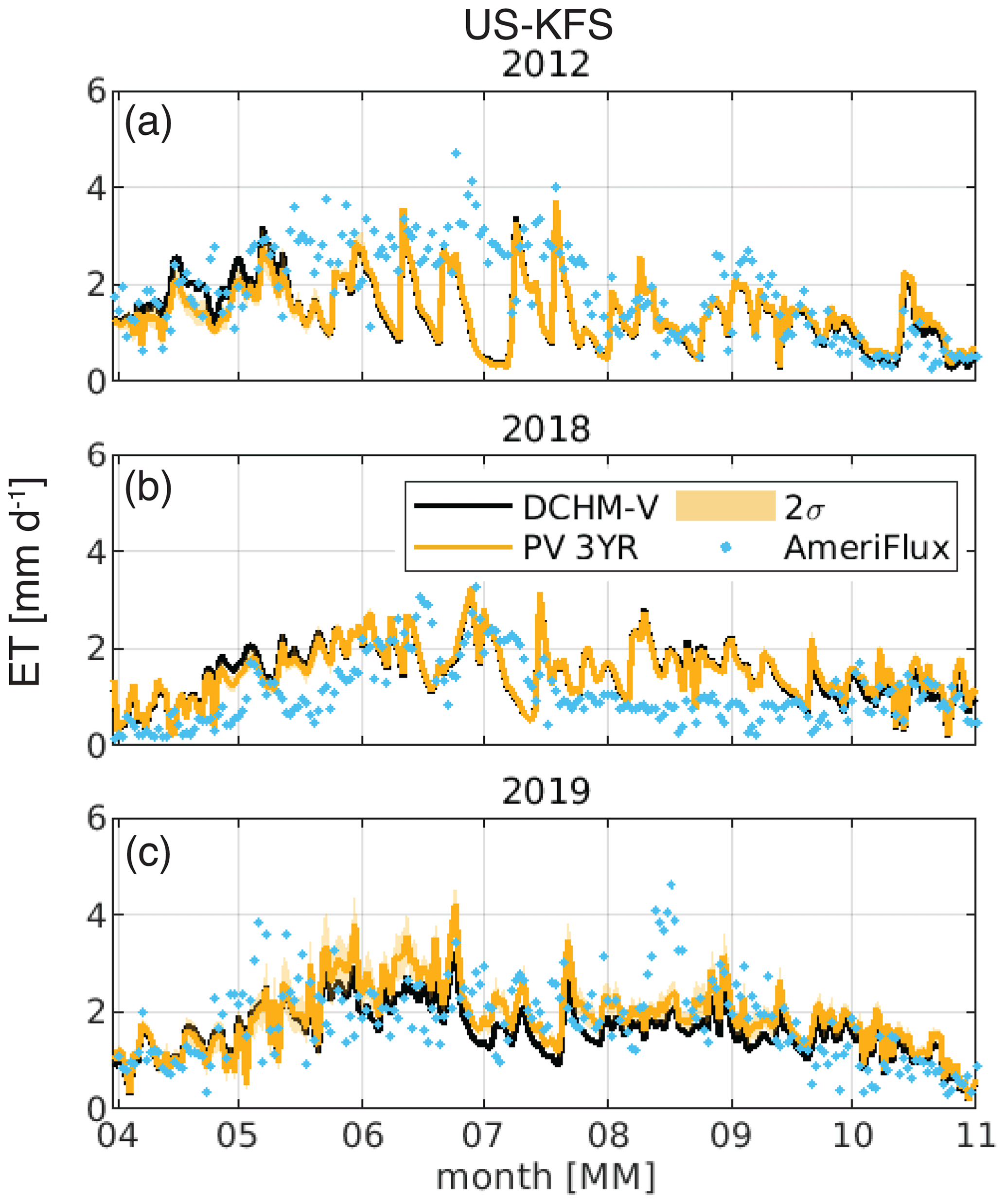
Figure 14 Daily evapotranspiration, ET, at US-KFS for a (a) flash drought year (2012), (b) drought year (2018), and (c) non-drought year (2019). The shaded area for the DCHM-PV simulations denotes 2 standard deviations. AmeriFlux ET is derived from latent heat measurements and shown as blue dots.

Daily ET estimated by the DCHM-PV matches well against AmeriFlux estimates at US-KFS during the flash drought and non-flash-drought years (Fig. 14). In 2012, the DCHM-PV ET agrees with AmeriFlux through mid-May. From late-May through July, the model results tend to fall below AmeriFlux until August when they once again agree. In the drought (2018) and non-drought (2019) years, the DCHM-PV ET appears to align with AmeriFlux throughout most of the season (Fig. 14b, c). While model estimates of ET are higher than flux tower measurements in 2019 at US-KLS, they compare favorably in 2012 and 2018 (Fig. S17). In contrast to model and flux tower comparisons at US-KFS and US-KLS, modeled ET agrees with AmeriFlux in 2019 (non-drought) but underestimates it during the summer months in 2012 (flash drought) and 2018 (drought) at US-Kon (Fig. S18). One explanation for the differences between model and tower ET data could be that water use by vegetation during flash drought is highly variable across sites; thus, the model is not able to represent all possible responses. Additionally, it is difficult for DCHM and other Earth system models to account for plant access to deep water stores (Giardina et al., 2023).

4 Discussion

4.1 Mechanisms controlling plant responses to drought

An objective of this work is to evaluate whether changes in phenology vs. changes in stomatal conductance have a stronger control on carbon uptake during flash drought (H2 and H3). Prior work has linked phenological responses to drought to changes in vegetation–atmosphere interactions (Lowman and Barros, 2018; Cui et al., 2017). Dynamically estimated FPAR and LAI tend to exert strong controls on the resulting GPP (Lowman and Barros, 2018). By updating phenological states using the phenology model, rather than forcing phenology with remotely sensed values, we were able to capture the plant growth response to water availability. When more water is available, the DCHM-PV simulation predicts higher values of FPAR and LAI and, thus, higher values of GPP. At the onset of flash drought, the DCHM-V and -PV respond faster than MODIS to changes in LAI and FPAR (Figs. 5, 6), leading to differences in modeled and remotely sensed GPP (Fig. 11). Moreover, regardless of the simulation, the rapidness of the change in LAI and FPAR is indicative of flash drought, which is in agreement with Zhang et al. (2020). Decreases in the phenological state due to the lack of soil water available to plants affected carbon and water exchanges, suggesting support for the third hypothesis (H3); however, decreases in stomatal conductance driven by increased VPD may compound the detrimental phenological effects.

While phenology is an important component to consider when simulating changes in transpiration and carbon uptake (Lowman and Barros, 2018; Flack-Prain et al., 2019), our results indicate that stomatal conductance is also critical for accurately representing these fluxes. Plants adaptively regulate their stomata during periods of water stress (Guo et al., 2020), and some have been demonstrated to maintain open stomata or even increase stomatal conductance under high-VPD conditions (Urban et al., 2017). Stomatal conductance shuts down under high VPD in the DCHM (Fig. 9), which does not account for the possibility of an adaptive stomatal regulation strategy. As GPP is directly dependent on stomatal conductance (Farquhar and Sharkey, 1982), the DCHM estimates of sub-daily GPP decrease in response to elevated VPD (Fig. S22). Moreover, changes in phenological growth state (i.e., LAI) occur across longer (e.g., seasonal) timescales than stomatal regulation (Katul et al., 2001), which controls carbon and water exchange at sub-daily timescales (Guo et al., 2020).

The differences between modeled and observed GPP and ET (Figs. 11, 14) suggest that there are mechanisms controlling plant responses to drought stress that are not accounted for within the DCHM. For example, the DCHM could be too strict with respect to representing the sensitivity of stomatal closure to elevated VPD for the Kansas study sites. There could also be plant- or climate-specific VPD dependence (Grossiord et al., 2020), plants could have access to stores of water not accounted for (Giardina et al., 2023), or both. Guo et al. (2020) showed that isohydricity (i.e., stomatal regulation) exists on a spectrum and that some plants are able to move along that spectrum at sub-daily timescales with varying environmental conditions, such as higher VPD. Given the high VPD in 2012 at our study sites (Figs. S5, S28, S29, and S30), DCHM estimated low stomatal conductance, and thus low GPP relative to AmeriFlux observations when under atmospheric water stress. This was evident in the slow reduction in GPP during May and June 2012 before reaching a minimum near the beginning of July, marking stomatal closure and a shift toward more isohydric behavior (Figs. 10, 11; Meinzer, 2002). Additionally, VPD estimated by DCHM using the NLDAS-2 Forcing File A atmospheric variables is higher during 2012 and 2018 and lower in 2019 than the AmeriFlux observations (Fig. S28), explaining some of the discrepancy between modeled and AmeriFlux GPP. As stomatal response to increasing VPD and resulting impacts on land–atmosphere water fluxes is more complex than how it is represented in LSMs (Vargas Zeppetello et al., 2023), future modeling studies should focus on how rising VPD drives stomatal closure across different vegetation types (Grossiord et al., 2020).

4.2 Surface and subsurface water movement

At the onset of flash drought, there is an increase in evaporative demand for water that leads to a temporary increase in surface evaporation (Lowman et al., 2023; Otkin et al., 2018). Once the soil and canopy reservoirs no longer contain enough water, evaporation shuts down. Despite evaporation tapering to zero during June and July of 2012 (Fig. S19), pulses of rainfall led to temporary rapid increases in rates of evaporation. Increased surface evaporation may reduce the amount of water infiltrating the soils. Across all three study sites, infiltration exceeded evaporation in the growing season in drought and non-drought years (Figs. 7, 10). During flash drought, infiltration totals were of a similar magnitude to evaporation totals. Thus, a decrease in total infiltration concurrent with increased evaporation may be an indicator of flash drought.

We found that it is important to consider the partitioning of ET when studying plant responses to flash drought. Accumulated monthly averages of transpiration as a fraction of evapotranspiration (T $/$ ET) showed a transition from at or above non-drought levels to at or below drought levels (Fig. 15). Excluding 2012, growing season transpiration rates averaged more than 50 % of total ET at US-KFS. This finding aligns with prior results from Hosseini et al. (2022), who used the Noah-MP LSM that also computes transpiration from root water uptake (Li et al., 2021). However, during the flash drought year, transpiration rates fell below 35 % of overall ET at US-KFS (Fig. 15a). Transpiration decreased by approximately 20 %–40 % from May to June at US-KLS and US-Kon (Fig. 15b, c). The rapid decline in transpiration rates can be attributed to the slowing of root water uptake due to the lack of available water and decreased stomatal conductance (Figs. S6 and S7). It is possible that the fluctuating T $/$ ET at US-Kon, modeled as a grassland, is indicative of an adaptation to the water stresses.

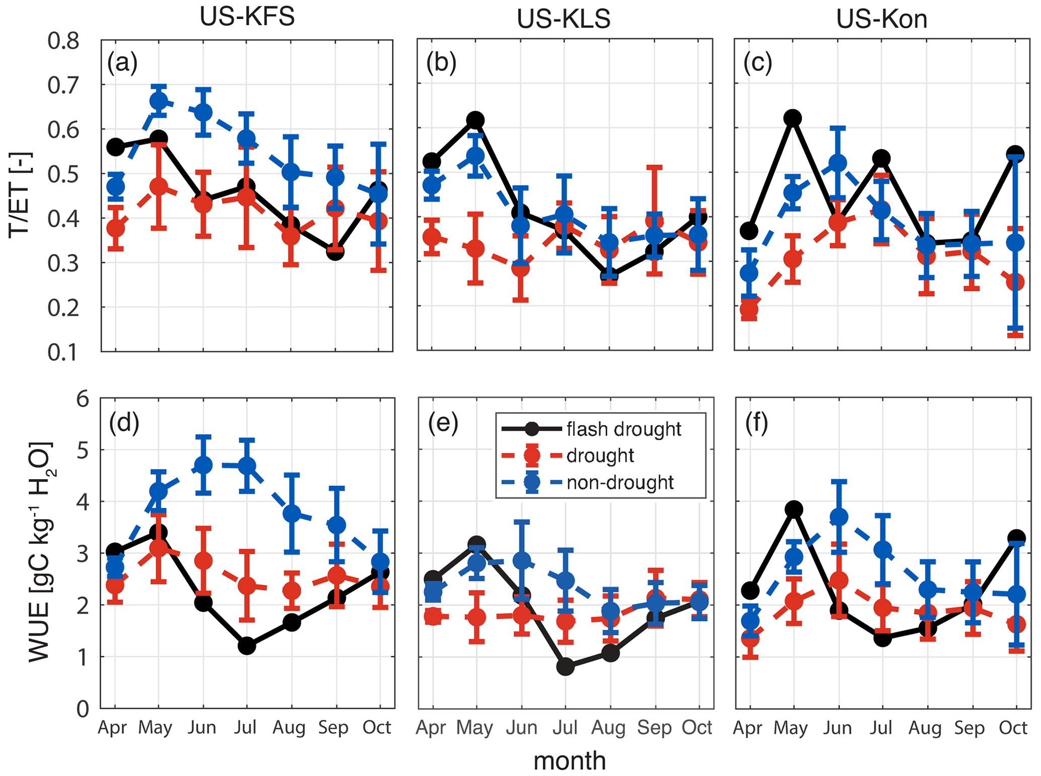
Figure 15 Ratio of transpiration to evapotranspiration, T $/$ ET (–), and water use efficiency, WUE (gC kg⁻¹ H₂O), for drought (red) and non-drought (blue) years compared to flash drought (black) for US-KFS (a, d), US-KLS (b, e), and US-Kon (c, f).

4.3 Linking carbon and water fluxes

Vegetation responses to water stress are apparent through fluctuations in GPP (Zhang and Yuan, 2020; Jin et al., 2019) and ET (Chen et al., 2019). Decreases in GPP occur when plants close their stomata, limiting gas exchange and affecting both rates of photosynthesis and transpiration. Transpiration is only one part of ET, so we must be careful not to directly link fluctuations in GPP with fluctuations in ET. Evaporation can still be high when there is little to no transpiration, but we find that GPP tends to follow the same trajectories as transpiration (Figs. 10 and 13 and Fig. S19a;  Beer et al., 2009).

Despite major reductions in infiltration and fluctuations in top-layer soil moisture during flash drought onset, modeled root water uptake indicated that plants were still pulling small amounts of water through their roots (Fig. S6), allowing transpiration to occur and preventing complete shutdown. With the ability to tap into water stores from deeper layers (Giardina et al., 2023) and small rates of transpiration still occurring, modeled carbon uptake is maintained (Fig. 11a, S15a and S16a). For example, ET decreased at US-KFS during July 2019 while experiencing a brief period of low rainfall (Fig. S19b), yet plants were able to maintain rates of GPP during this period due to the amount of available water in soils from the excessive precipitation during May and June (Figs. S1c, S2c, and S3c). Although GPP drastically slowed, it did not stop. The decreases in simulated GPP due to flash drought during June and July 2012 were consistent in terms of magnitude with decreases found in recent studies (Yao et al., 2022; Poonia et al., 2022; Zhang et al., 2020).

Changes in the ratios of T $/$ ET when compared with simultaneous changes in WUE indicated that plants that have higher rates of transpiration are more efficient in their water use (Fig. 15). We found that plants are more efficient during non-drought periods and are less efficient during flash drought onset. WUE at all sites started off in 2012 at above the average non-drought levels and increased from April to May. However, from May to July, WUE at all sites fell from values above non-drought years to more than 1 standard deviation below drought years. With GPP differences being more substantial than ET between flash drought and non-flash-drought periods (Fig. 10), sub-seasonal reductions in WUE were attributed to the losses in GPP. Reductions in WUE from above non-drought conditions to below drought conditions, e.g., the 60 %–70 % reduction from May to July in 2012, appeared to be a feature of flash drought onset (Fig. 15d, e, f).

4.4 Uncertainty in vegetation responses

Three different assimilation strategies were used to evaluate how uncertainty propagates from the predictive phenology routine through to the DCHM-PV model outputs (Fig. 3). The 2003–2005 period represented “average” conditions, as it spanned periods of below- and above-average precipitation. Compared with the single-year assimilation periods (WET and DRY), the uncertainty ranges in model parameters were smaller in the 3YR assimilation period. These results are consistent with Lowman and Barros (2018) in that uncertainty in phenology shrank during dry periods. Future studies should use an assimilation period encompassing multiple precipitation regimes (i.e., multiyear inference period) to best represent the variability in climatological conditions, as it leads to reduced uncertainty in model outputs. However, if the intent of a future study is to investigate vegetation responses to extreme events in a changing climate (e.g., Kirono et al., 2020; Pearson et al., 2013), it may be appropriate to use inference periods encompassing extreme wet or dry conditions. For example, one could fit parameters to a dry regime to investigate how plants accustomed to today's average conditions will function in a future climate in which drier conditions are expected.

The γ parameter values, which drive plant growth in the DCHM-PV, were lower in the 3YR assimilation period for all three test sites compared with simulations from drought and wet years. Daily standard deviations in LAI across simulations were approximately 0.5 m² m⁻² during the growing season of a wet year, but they shrank to values of 0.2 m² m⁻² at the onset of flash drought and to less than 0.1 m² m⁻² during peak flash drought. The lower ensemble spread during the flash drought period corresponded with winter phenological variability when plants are dormant. Similarly, decreases in uncertainty in estimates of GPP and ET during the flash drought period fell to winter levels, implying that variability in plant life stage and functionality are similar in drought periods and dormant months.

4.5 Model performance and limitations

Our modeling approach permits direct comparisons of remotely sensed and ground observations to physically derived estimates. However, it should be noted that, when analyzing the DCHM outputs against remotely sensed and eddy covariance measurements, we are comparing data across temporal and spatial scales. The flux towers exist within a 4 km × 4 km region defined by the Stage-IV spatial grid cell used in DCHM. Flux tower spatial extents range from a couple of hundred meters to a few kilometers (Baldocchi, 2003; Schmid, 1994), making the 4 km grid cell near the maximum range. Sub-grid-scale heterogeneity can lead to considerable discrepancies between parameterized and actual fluxes (Schmid, 1994). One explanation for why flux tower data differ from model output is that the flux tower estimates incorporate a variety of vegetation types within the fetch contributing to the vertical fluxes, rather than the single vegetation type used within the model. Additionally, the size and orientation of the contributing fetch varies in time depending on measurement height and turbulent fluxes (Chu et al., 2021). Differences between model outputs and remote sensing observations could be due to discrepancies in the land cover classification, a result of interpolating MODIS land cover at 500 m to the 4 km grid cell used in the DCHM. Regardless of the classification differences, the spectral reflectance method used by MODIS is inherently different from the predictive phenology routine used in the DCHM-PV, specifically in that it cannot account for how soil water availability influences vegetation growth (Lowman and Barros, 2018).

Regardless of vegetation type, the physically based DCHM-PV model compares favorably against MODIS LAI during flash drought and non-drought at US-KFS and US-KLS, whereas it underestimates those sites during drought (Fig. 6). The higher DCHM-PV model estimates of FPAR and LAI during summer 2019 could be due to the model accounting for excess water availability and other meteorological conditions favorable for growth (e.g., temperature and VPD). In contrast, MODIS estimates of FPAR and LAI are based on radiative transfer models using bidirectional reflectance of incoming radiation from the red and NIR bands (Myneni et al., 2015; Yan et al., 2016). Our model performance against MODIS is similar to that found in Hosseini et al. (2022), who also used a predictive phenology model coupled with Noah-MP.

Daily GPP from DCHM tends to match the magnitude of MODIS and AmeriFlux GPP at US-KFS throughout much of the growing season, but it underestimates June and July observations in 2012 (flash drought) and 2018 (drought). MODIS GPP is directly dependent on observations of FPAR (Running et al., 2015), and, generally, MODIS overestimates GPP compared with eddy covariance flux tower data (Heinsch et al., 2006; Running et al., 2004). However, AmeriFlux estimates of GPP during June and early July of 2012 and 2018 are above estimates from MODIS. This suggests that plants are able to maintain higher levels of GPP during drought and flash drought than what can be recreated using land surface models and satellite remote sensing. In some cases, vegetation can reallocate already processed carbon to their roots when under drought stress, thereby mitigating GPP losses (Ingrisch et al., 2020). However, differences in the DCHM-PV and AmeriFlux GPP cannot be fully attributed to carbon reallocation, as the Noah-MP model accounts for carbon reallocation and similarly underestimated GPP compared with flux tower data (Hosseini et al., 2022). The DCHM-PV, which does not account for carbon reallocation, responds to drought and flash drought differently than what is observed at flux tower sites. It matches better with AmeriFlux data during 2012, the flash drought year, at US-KFS and US-KLS compared with 2018, a drought year (Figs. 11 and S15).

Another explanation for the discrepancies between modeled and flux tower data could be that models may not be able to fully represent how vegetation can maintain transpiration by accessing groundwater or deep soil moisture, ultimately biasing models towards more severe effects of drought on vegetation (Giardina et al., 2023). The DCHM has similar soil moisture profiles to NLDAS-2, derived from Noah-LSM, and Hosseini et al. (2022), who used Noah-MP configurations, for both the 2012 flash drought and the 2018 drought. The DCHM estimates of GPP are often less than 50 % of AmeriFlux GPP in 2012 and 2018. The model results from the Noah-MP similarly underestimate GPP and overestimate soil moisture during these drought periods (Hosseini et al., 2022), suggesting that access to deep water reserves could be responsible for these differences (Giardina et al., 2023).

4.6 Implications for land surface models

Capturing phenological responses and subsequent changes in carbon and water fluxes within a physically based model is not without its limitations. Assimilating plant phenology into land surface models (e.g., the DCHM-V or Noah-MP) can improve estimates of GPP and ET (Hosseini et al., 2022; Xu et al., 2021; Mocko et al., 2021; Kumar et al., 2019). However, our findings indicate that improved phenology cannot alone account for vegetation adaptations to water stress, including the ability to access water in ways that current LSMs cannot (Giardina et al., 2023). Future studies would benefit from improved estimates of root water uptake, as it is directly linked to the amount of available water for transpiration. An emphasis should be placed on understanding how plants are able to tap into different stores of water to continue exchanging water and carbon despite lower precipitation or increased VPD. Additionally, stomata control the movement of water and carbon, affecting GPP and water use efficiency (Lawson and Vialet-Chabrand, 2019). Sub-daily-scale stomatal conductance reduces to zero in response to increased VPD, leading to similar reductions in modeled GPP (Figs. 9 and S22). This limitation of DCHM could explain why AmeriFlux GPP tends to be higher than the modeled GPP. Accounting for growing season adaptations to regulate stomatal sensitivity to drought stress, as observed by Guo et al. (2022), may improve model accuracy.

Improvements made to the phenological states of the entire plant, rather than just the leaf phenology, could enhance the representation of water movement through plants under water stress conditions. Different vegetation types have their own root characteristics, leading to distinct hydraulic tendencies under variable water regimes and atmospheric conditions, which distinguish whether vegetation is more likely to survive or recover from drought (McDowell et al., 2008; Martínez-Vilalta et al., 2002). Hydraulic strategies may vary by species within a single location (Liu et al., 2020), so the generalization of water use strategy by PFT in hydrologic models represents the average tendency of vegetation to regulate water. The changing phenological state of root systems likely plays an important role in root water uptake (McCormack et al., 2014). Moreover, models that can account for different vegetation strategies, such as the reallocation of carbon storage and belowground respiration during drought, may provide a better understanding of mechanisms driving drought resiliency and changes in carbon uptake during drought (Ingrisch et al., 2020; Sanaullah et al., 2012). These types of mechanisms could explain how a warm and wet spring mitigated the effects of the 2012 flash drought on GPP losses (Wolf et al., 2016).

5 Conclusions

To address how water stresses affect carbon and water cycling, we implemented a 1-D version of the DCHM-V coupled to a predictive phenology model and analyzed vegetation–atmosphere water and carbon exchanges during flash drought, drought, and non-drought periods. The modeling procedure first required running the DCHM-V with phenology updates from remotely sensed observations of FPAR and LAI. After coupling the predictive phenology model to the DCHM-V, we generated ensembles of model parameters and ran Monte Carlo simulations of the DCHM-PV with concurrent meteorological conditions. We ran three simulations using three distinct assimilation periods for three different sites in Kansas. Uncertainty in model parameters and outputs is reduced when a 3-year assimilation period, considering average conditions, is used.

The effects of water stress on phenology, infiltration, stomatal conductances, and WUE were similar across all three study sites and helped to distinguish flash drought conditions from non-flash-drought conditions. Our findings indicated that both phenology and stomatal conductance play an important role in controlling vegetation responses to extreme drought (H2 and H3). Decreased infiltration due to increased days between precipitation during flash drought resulted in less soil water available for plant use (H1 and H2). High vapor pressure deficit led to stomatal closure within the model. With stomata closed, root uptake, transpiration, and carbon assimilation reduced to dormant levels. This led to reductions in WUE during the flash drought that were more than 1 standard deviation below other drought periods (H2). FPAR and LAI also decreased during the flash drought but did not exert as strong of a control on reductions in GPP as observed with changes in stomatal conductance that resulted from increased VPD.

The seasonal timing of the flash drought was particularly detrimental because the rapid dry down occurred during the peak growing season. The amount of water available during the growing season has a major influence on vegetation activity. In this region of the US, droughts can reduce monthly carbon assimilation by half compared with non-drought periods, while flash droughts are even more detrimental to the overall carbon budget. This has major implications for annual crop yields as well as for the carbon uptake capacity of grasslands and savannas that cover much of the Midwestern US. Future modeling studies should investigate how different vegetation types alter their water use strategies in response to different water stresses by including (1) adaptive stomatal regulation under elevated VPD, (2) access to deep stores of water in soils, and (3) wider ranges of plant functional types and climatological regimes.