Adjoint subordination to calculate backward travel time probability of pollutants in water with various velocity resolutions

Backward probabilities, such as the backward travel time probability density function for pollutants in natural aquifers/rivers, have been used by hydrologists for decades in water quality applications. Calculating these backward probabilities, however, is challenging due to non-Fickian pollutant transport dynamics and velocity resolution variability at study sites. To address these issues, we built an adjoint model by deriving a backward-in-time fractional-derivative transport equation subordinated to regional flow, developed a Lagrangian solver, and applied the model/solver to trace pollutant transport in diverse flow systems. The adjoint model subordinates to a reversed regional flow field, transforms forward-in-time boundaries into either absorbing or reflective boundaries, and reverses the tempered stable density to define backward mechanical dispersion. The corresponding Lagrangian solver efficiently projects backward super-diffusive mechanical dispersion along streamlines. Field applications demonstrate the adjoint subordination model's success with respect to recovering release history, groundwater age, and pollutant source locations for various flow systems. These include systems with upscaled constant velocity, nonuniform divergent flow fields, or fine-resolution velocities in a nonstationary, regional-scale aquifer, where non-Fickian transport significantly affects pollutant dynamics and backward probabilities. Caution is needed when identifying the phase-sensitive (aqueous vs. absorbed) pollutant source in natural media. The study also explores possible extensions of the adjoint subordination model for quantifying backward probabilities of pollutants in more complex media, such as discrete fracture networks.

1 Introduction

Backward probabilities of pollutants in natural aquifers/rivers, such as the backward travel time probability (BTTP) density function, have been used by hydrologists for decades in water quality applications. For example, the BTTP estimates the time that contaminants take to reach a sampling location (e.g., a monitoring well screen or stream sampling location) from their source(s) (Neupauer and Wilson, 2001; Ponprasit et al., 2023). It provides useful insights for water management, remediation, and assessment. For instance, a common application of BTTP is to recover contamination history and identify responsible parties, where the BTTP's peak captures the most likely release time of contaminants from the source (Skaggs and Kabala, 1994; Woodbury and Ulrych, 1996; Woodbury et al., 1998; Sun et al., 2006a, b; Jha and Datta, 2015; Yeh et al., 2016; Jamshidi et al., 2020; Chen et al., 2023). The BTTP can also be used to date groundwater, as it characterizes the age distribution of groundwater due to borehole mixture and/or hydrodynamic dispersion in regional-scale aquifers (Weissmann et al., 2002; Cornaton and Perrochet, 2006; LaBolle et al., 2006; Zinn and Konikow, 2007a, b; Janssen et al., 2008; McMahon et al., 2008; Maxwell et al., 2016; Ponprasit et al., 2022; Mao et al., 2023). In addition, the BTTP provides a more comprehensive method to assess aquifer vulnerability than classical statistics-based approaches through the generation of three-dimensional (3D), transient vulnerability maps for groundwater to non-point-source contamination (Fogg et al., 1999; Zhang et al., 2018). The BTTP can also be used to estimate solute concentration trends (Green et al., 2014) as well as rates of oxygen and nitrate reduction in regional groundwater settings (Green et al., 2016). These diverse applications underscore the need for a general BTTP model, which is the focus of this study.

There are two main challenges in numerically quantifying backward probabilities, including the BTTP, for contaminant transport in surface water and groundwater. Firstly, a novel model is required to address the impact of complex transport dynamics of contaminants on the BTTP. Previous BTTP models, usually based on inverse or backward advection–dispersion equations (ADEs), assumed Fickian diffusion of contaminants, where the plume variance grows linearly over time; see the extensive review by Moghaddam et al. (2021). Real-world contaminant transport, however, is often non-Fickian at various scales, exhibiting either slower-than-linear temporal plume variance growth (known as “sub-diffusion”) or faster-than-linear growth (known as “super-diffusion”), as recently reviewed by Guo et al. (2021). Particularly, super-diffusion can be driven by factors like turbulence or flooding events in streams (Phillips et al., 2013; Boano et al., 2014), preferential flow pathways consisting of fractures in fractured porous media (Reeves et al., 2008), or high-permeability paleochannels within alluvial deposits (Bianchi et al., 2016). Sub-diffusion is more common in natural water systems due to pervasive solute retention or storage mechanisms such as physical/chemical sorption–desorption, heterogeneous advection (meaning a broad range of advective velocities), and multi-rate mass exchange between mobile and relatively immobile flow zones (Haggerty et al., 2000; Zhou et al., 2021). Classical Fickian-diffusion models cannot effectively capture super-/sub-diffusive non-Fickian transport when the velocity field lacks sufficient resolution (e.g., coarser than the centimeter scale; see Zheng et al., 2011) or when the model underestimates the spatial interconnectivity of high-permeability deposits (Yin et al., 2020). To address this issue, various nonlocal transport models, which are typically non-Markovian models considering the spatiotemporal memory during solute transport, have been developed to efficiently simulate forward-in-time non-Fickian transport (Neuman and Tartakovsky, 2009). However, their corresponding BTTP models have remained less explored (Zhang et al., 2022; Zhang, 2022).

The second challenge is how to integrate the observed velocity field, which often varies significantly in resolution across field sites, into backward probability calculations, including the BTTP. Many field sites lack extensive hydrologic data, necessitating an upscaled BTTP model capable of operating with coarsely resolved velocity or uniform velocity fields. Contrarily, well-studied sites with abundant geologic and hydrologic data should incorporate detailed spatiotemporal velocity distributions to enhance the BTTP calculation reliability. Ideally, an efficient BTTP model should seamlessly incorporate velocity fields without resolution constraints.

To fill these two knowledge gaps, this study proposes an adjoint subordination approach by deriving a backward-in-time model (also known as an “adjoint”) for the 3D time fractional-derivative equation (FDE) subordinated to water flow with or without a highly resolved velocity field. Such a forward-in-time FDE was proposed by Zhang et al. (2015) as a general forward model for pollutant transport in various geological media. Notably, two other vector nonlocal transport models, the well-known continuous-time random walk (CTRW) framework (Hansen and Berkowitz, 2020) and the multi-scaling FDE model (Zhang, 2022), can also incorporate local velocity variations into non-Fickian diffusion. The CTRW framework allows for various memory functions to define solute transition times, but it does not separate sub-diffusion (due to solute retention) and super-diffusion (e.g., due to preferential flow paths) (Lu et al., 2018). This study selects the subordinated time-FDE, as explained in Sect. 2, for two key reasons: (i) it can capture both sub-diffusion (using the time fractional derivative) and sub-grid super-diffusion (via subordination, distinct from the space fractional derivative) and (ii) it offers computational efficiency compared with the multi-scaling FDE (introduced in Sect. 4).

The remainder of this work is structured as follows: Sect. 2 applies a sensitivity analysis approach to build the adjoint of the subordinated time-FDE and then develops and validates a Lagrangian solver of the resulting BTTP model; Sect. 3 checks the feasibility of the adjoint model and its solver by quantifying the BTTP, identifying the release history of contaminants in an alluvial aquifer and a river with uniform velocity, and calculating groundwater ages dated using environmental tracers in a regional-scale alluvial aquifer with fine velocity resolution; Sect. 4 discusses the identification of contaminant source locations based on the backward location probability (BLP) density function and extends the backward probability model; and Sect. 5 draws the main conclusions.

2 Methodology development

This section derives the model and solver for backward-in-time subordination to water flow in heterogeneous media. The concept of subordination to regional flow was initially proposed by Baeumer et al. (2001) and later extended to multidimensional flow by Zhang et al. (2015). Subordination is a statistical method that randomizes the operational time experienced by individual particles in a random process (Feller, 1971). When applied to regional flow, this process captures fast displacement of pollutant particles along streamlines during the randomized operational time, as shown and explained in the following model (Eq. 1a).

2.1 Forward and backward models

2.1.1 The 3D transport and adjoint models

We propose the following 3D subordinated time-FDEs to track pollutants in streams and aquifers with vector velocity, after adding source/sink and reaction terms and initial/boundary conditions in the vector model proposed by Zhang et al. (2015):

$$\begin{array}{}\text{(1a)}& {\displaystyle }\begin{array}{rl}& b{\displaystyle \frac{\partial \left(\mathit{\theta }C\right)}{\partial t}}+\mathit{\beta }{\displaystyle \frac{{\partial }^{\mathit{\gamma },\mathit{\lambda }}\left(\mathit{\theta }C\right)}{\partial t^{\mathit{\gamma },\mathit{\lambda }}}}=-{\mathrm{\nabla }}_{\mathit{V}}\left(\mathit{\theta }C\right)\\ & +{\mathit{\sigma }}^{*}{\left({\mathrm{\nabla }}_{\mathit{V}}\right)}^{\mathit{\alpha },\mathit{\kappa }}\left(\mathit{\theta }C\right)+q_{\mathrm{I}}{C}_{\mathrm{I}}-q_{o}C-\mathit{\theta }rC,\end{array}\text{(1b)}& {\displaystyle }C\left(\mathit{x},t=\mathrm{0}\right)={\displaystyle \frac{M_{\mathrm{0}}}{\mathit{\theta }}}\mathit{\delta }\left(\mathit{x}-{\mathit{x}}_{\mathrm{0}}\right),\text{(1c)}& {\displaystyle }{\left.C\left(\mathit{x},t\right)\right|}_{{\mathit{\xi }}_{\mathrm{1}}}=g_{\mathrm{1}}\left(t\right),\text{(1d)}& {\displaystyle }{\left.\left[{\mathit{\sigma }}^{*}{\left({\mathrm{\nabla }}_{\mathit{V}}\right)}^{\mathit{\alpha }-\mathrm{1},\mathit{\kappa }}\left(\mathit{\theta }C\right)\right]\cdot {\mathit{n}}_{\mathrm{2}}\right|}_{{\mathit{\xi }}_{\mathrm{2}}}=g_{\mathrm{2}}\left(t\right),\text{(1e)}& {\displaystyle }{\left.\left[V\left(\mathit{x},t\right)\mathit{\theta }C-{\mathit{\sigma }}^{*}{\left({\mathrm{\nabla }}_{\mathit{V}}\right)}^{\mathit{\alpha }-\mathrm{1},\mathit{\kappa }}\left(\mathit{\theta }C\right)\right]\cdot {\mathit{n}}_{\mathrm{3}}\right|}_{{\mathit{\xi }}_{\mathrm{3}}}=g_{\mathrm{3}}\left(t\right).\end{array}$$

Here, C [ML⁻³] denotes the solute concentration, b (=0 or 1) [dimensionless] is a factor controlling the type of the time FDE, θ [dimensionless] is the effective porosity, β [T^γ−1] is the fractional capacity coefficient, σ^* [L] is a scaling factor for subordination, V [LT⁻¹] is the velocity vector (note that all vectors in this paper are formatted in bold italic), ∇_V is an advection operator defined via ∇_V =∇(VC), q_I [T⁻¹] is the source inflow rate, C_I is the inflow concentration, q_O is the sink outflow rate, r [T⁻¹] is the first-order decay constant, M₀ is the initial source mass, g_i ($i=\mathrm{1},\mathrm{2},\mathrm{3}$) is a known function at the type-i boundary (to define the constant concentration or pollutant flux at the boundary), ξ_i ($i=\mathrm{1},\mathrm{2},\mathrm{3}$) is the domain of the type-i boundary, x [L] denotes the spatial coordinate, t [T] is the (forward) time, and n₂ and n₃ are outward unit normal vectors on the respective type-2 and type-3 boundaries. We refer to Eq. (1a) as the subordinated fractional-derivative equation (S-FDE).

The S-FDE (Eq. 1a) captures the concurrent sub-diffusion and super-diffusion, driven by different mechanisms represented by different terms. In Eq. (1a), the symbol $\frac{{\partial }^{\mathit{\gamma },\mathit{\lambda }}}{\partial t^{\mathit{\gamma },\mathit{\lambda }}}$, which is the mixed Caputo fractional derivative with an index γ [dimensionless] ($\mathrm{0}<\mathit{\gamma }\le \mathrm{1})$ and a temporal truncation parameter λ [T⁻¹] (Baeumer et al., 2018), defines sub-diffusion due to solute retention. The operator ${\left({\mathrm{\nabla }}_{\mathit{V}}\right)}^{\mathit{\alpha },\mathit{\kappa }}$, representing subordination to the flow field with an index α [dimensionless] ($\mathrm{1}<\mathit{\alpha }\le \mathrm{2})$ for the tempered stable density (with the maximum possible positive skewness ${\mathit{\beta }}^{*}=+\mathrm{1})$ and a spatial truncation parameter κ [L⁻¹], describes fast downstream displacements. It is worth noting that pollutant particles undergo advective displacement controlled by local mean velocity, with individual particles migrating along various flow paths in a heterogeneous medium, leading to random mechanical dispersion due to local speeds deviating from the mean velocity. Equation (1a) assumes a (tempered) α-stable density distribution for random mechanical dispersive jumps, rescaled by the mean local velocity. This (tempered) α-stable density encompasses both Gaussian and power-law densities as two end-members. Therefore, subordination to regional flow extends standard symmetric mechanical dispersion to nonsymmetric, super-diffusive mechanical dispersion along streamlines, driven by local velocity variations, like super-diffusion along preferential flow paths. Notably, if molecular diffusion is not negligible, it can be included in Eq. (1), combining with the subordination term responsible for mechanical dispersion to define hydrodynamic dispersion.

To derive the backward model for the S-FDE (Eq. 1) using the adjoint approach (Neupauer and Wilson, 2001), we first convert it to the model governing the state sensitivity $\mathit{\varphi }=\frac{\partial C}{\partial f}$, where f is a system parameter and is selected as the initial mass M₀, as in Neupauer and Wilson (2001) and Zhang (2022). This can be done by taking the first-order derivative of each term in the S-FDE (Eq. 1) with respect to M₀, which leads to the following:

$$\begin{array}{}\text{(2a)}& {\displaystyle }\begin{array}{rl}& \left(b{\displaystyle \frac{\partial }{\partial t}}+\mathit{\beta }{\displaystyle \frac{{\partial }^{\mathit{\gamma },\mathit{\lambda }}}{\partial t^{\mathit{\gamma },\mathit{\lambda }}}}\right)\left(\mathit{\theta }\mathit{\varphi }\right)=-{\mathrm{\nabla }}_{\mathit{V}}\left(\mathit{\theta }\mathit{\varphi }\right)\\ & +{\mathit{\sigma }}^{*}{\left({\mathrm{\nabla }}_{\mathit{V}}\right)}^{\mathit{\alpha },\mathit{\kappa }}\left(\mathit{\theta }\mathit{\varphi }\right)-\left(q_o+\mathit{\theta }r\right)\mathit{\varphi },\end{array}\text{(2b)}& {\displaystyle }\mathit{\varphi }\left(\mathit{x},t=\mathrm{0}\right)={\displaystyle \frac{\partial C\left({\mathit{x}}_i\right)}{\partial M_{\mathrm{0}}}}={\displaystyle \frac{\mathrm{1}}{\mathit{\theta }}}\mathit{\delta }\left(\mathit{x}-{\mathit{x}}_{\mathrm{0}}\right),\text{(2c)}& {\displaystyle }{\left.\mathit{\varphi }\left(\mathit{x},t\right)\right|}_{{\mathit{\xi }}_{\mathrm{1}}}=\mathrm{0},\text{(2d)}& {\displaystyle }{\left.\left[{\mathit{\sigma }}^{*}{\left({\mathrm{\nabla }}_{\mathit{V}}\right)}^{\mathit{\alpha }-\mathrm{1},\mathit{\kappa }}\left(\mathit{\theta }\mathit{\varphi }\right)\right]\cdot {\mathit{n}}_{\mathrm{2}}\right|}_{{\mathit{\xi }}_{\mathrm{2}}}=\mathrm{0},\text{(2e)}& {\displaystyle }{\left.\left[V\mathit{\theta }\mathit{\varphi }-{\mathit{\sigma }}^{*}{\left({\mathrm{\nabla }}_{\mathit{V}}\right)}^{\mathit{\alpha }-\mathrm{1},\mathit{\kappa }}\left(\mathit{\theta }\mathit{\varphi }\right)\right]\cdot {\mathit{n}}_{\mathrm{3}}\right|}_{{\mathit{\xi }}_{\mathrm{3}}}=\mathrm{0}.\end{array}$$

Here, the time fractional derivative operator commutes.

We then incorporate the adjoint state of the concentration in the S-FDE (Eq. 2a) by taking the inner product of each term of Eq. (2a) with an arbitrary function A, which represents the adjoint state:

$$\begin{array}{}\text{(3)}& \begin{array}{rl}& {\int }_{\mathrm{0}}^T{\int }_{\mathrm{\Omega }}\left[Ab{\displaystyle \frac{\partial \left(\mathit{\theta }\mathit{\varphi }\right)}{\partial t}}+A\mathit{\beta }{\displaystyle \frac{{\partial }^{\mathit{\gamma },\mathit{\lambda }}}{\partial t^{\mathit{\gamma },\mathit{\lambda }}}}\left(\mathit{\theta }\mathit{\varphi }\right)+A{\mathrm{\nabla }}_{\mathit{V}}\left(\mathit{\theta }\mathit{\varphi }\right)\right.\\ & \left.-A{\mathit{\sigma }}^{*}{\left({\mathrm{\nabla }}_{\mathit{V}}\right)}^{\mathit{\alpha },\mathit{\kappa }}\left(\mathit{\theta }\mathit{\varphi }\right)+A\left(q_o+\mathit{\theta }r\right)\mathit{\varphi }\right]\mathrm{d}\mathrm{\Omega }\mathrm{d}t=\mathrm{0},\end{array}\end{array}$$

where Ω denotes the whole model domain. Afterward, through sensitivity analysis, we derive the backward model (please refer to Appendix A for details):

$$\begin{array}{}\text{(4a)}& {\displaystyle }\begin{array}{rl}& b{\displaystyle \frac{\partial \left(\mathit{\theta }A\right)}{\partial s}}+\mathit{\beta }{\displaystyle \frac{{\partial }^{\mathit{\gamma },\mathit{\lambda }}\left(\mathit{\theta }A\right)}{\partial s^{\mathit{\gamma },\mathit{\lambda }}}}={\mathrm{\nabla }}_{\mathit{V}}\left(\mathit{\theta }A\right)-\mathit{\theta }{\mathit{\sigma }}^{*}{\left({\mathrm{\nabla }}_{\overleftarrow{V}}\right)}^{\stackrel{\mathrm{‾}}{\mathit{\alpha }},\mathit{\kappa }}A\\ & -\left(q_{\mathrm{I}}+\mathit{\theta }r\right)A+{\displaystyle \frac{\partial h}{\partial C}},\end{array}\text{(4b)}& {\displaystyle }A\left(\mathit{x},s\right){\mathrm{|}}_{s=\mathrm{0}}=\mathrm{0},\text{(4c)}& {\displaystyle }{\left.A\left(\mathit{x},s\right)\right|}_{{\mathit{\xi }}_{\mathrm{1}}}=\mathrm{0},\text{(4d)}& {\displaystyle }{\left.\left[-A\mathit{\theta }V+{\mathit{\sigma }}^{*}\mathit{\theta }{\left({\mathrm{\nabla }}_{\mathit{V}}\right)}^{\stackrel{\mathrm{‾}}{\mathit{\alpha }-\mathrm{1}},\mathit{\kappa }}\left(A\right)\right]\cdot {\mathit{n}}_{\mathrm{2}}\right|}_{{\mathit{\xi }}_{\mathrm{2}}}=\mathrm{0},\text{(4e)}& {\displaystyle }{\left.\left[{\mathit{\sigma }}^{*}\mathit{\theta }{\left({\mathrm{\nabla }}_{\mathit{V}}\right)}^{\stackrel{\mathrm{‾}}{\mathit{\alpha }-\mathrm{1}},\mathit{\kappa }}\left(A\right)\right]\cdot {\mathit{n}}_{\mathrm{3}}\right|}_{{\mathit{\xi }}_{\mathrm{3}}}=\mathrm{0}.\end{array}$$

Here, s ($=T-t)$ represents backward time (with T as the detection time), and the operator ${\left({\mathrm{\nabla }}_{\overleftarrow{V}}\right)}^{\stackrel{\mathrm{‾}}{\mathit{\alpha }},k}$ denotes subordination to the reversed flow field $\left(\overleftarrow{V}\right)$ with a tempered α-stable density characterized by maximum negative skewness (${\mathit{\beta }}^{*}=-\mathrm{1}$), indicating fast displacements from downstream to upstream during backtracking. The initial condition (Eq. 4b) $A\left(\mathit{x},t\right){\mathrm{|}}_{t=T}=A\left(\mathit{x},s\right){\mathrm{|}}_{s=\mathrm{0}}=\mathrm{0}$ and the boundary conditions Eq. (4c)–(4e) are obtained by making sure that the remaining terms in Eq. (A6) in Appendix A define the following marginal sensitivity:

$$\begin{array}{}\text{(5)}& \begin{array}{rl}& {\displaystyle \frac{\mathrm{d}P}{\mathrm{d}{M}_{\mathrm{0}}}}=\\ & {\int }_{\mathrm{\Omega }}\left\{\left[\left(Ab\mathit{\theta }\right){\mathrm{|}}_{t=\mathrm{0}}+\mathit{\theta }{\mathrm{|}}_{t=\mathrm{0}}\mathit{\beta }{I}_{-}^{\mathrm{1}-\mathit{\gamma },\mathit{\lambda }}\left(A\right){\mathrm{|}}_{t=\mathrm{0}}\right]{\displaystyle \frac{\partial C_i}{\partial M_{\mathrm{0}}}}\right\}\mathrm{d}\mathrm{\Omega }.\end{array}\end{array}$$

Therefore, to convert the forward-in-time S-FDE (1) to its backward counterpart (Eq. 4), we need to (i) reverse the flow field, (ii) convert the source/sink terms and boundary conditions, and (iii) reverse the skewness in the stable density defining backward mechanical dispersive jumps. The first two changes were identified before by Neupauer and Wilson (2001) for the classical ADE (although the exact forward–backward transition is new here), and the last change is new. In the following, we name the backward-in-time model (Eq. 4) as the adjoint S-FDE.

2.1.2 The 1D simplifications

The 1D simplification of the vector forward-in-time S-FDE (Eq. 1) takes the following form:

$$\begin{array}{c}{\displaystyle }\begin{array}{rl}b{\displaystyle \frac{\partial \left(\mathit{\theta }C\right)}{\partial t}}& +\mathit{\beta }{\displaystyle \frac{{\partial }^{\mathit{\gamma },\mathit{\lambda }}\left(\mathit{\theta }C\right)}{\partial t^{\mathit{\gamma },\mathit{\lambda }}}}=-{\displaystyle \frac{\partial \left(V\mathit{\theta }C\right)}{\partial x}}\\ & +{\mathit{\sigma }}^{*}{\left({\displaystyle \frac{\partial }{\partial x}}\right)}_V^{\mathit{\alpha },\mathit{\kappa }}\left(\mathit{\theta }C\right)+q_{\mathrm{I}}{C}_{\mathrm{I}}-q_{o}C-\mathit{\theta }rC,\end{array}\\ {\displaystyle }C\left(x,t=\mathrm{0}\right)={\displaystyle \frac{M_{\mathrm{0}}}{\mathit{\theta }}}\mathit{\delta }(x-x_{\mathrm{0}}),\\ {\displaystyle }{\left.C(x,t)\right|}_{{\mathit{\xi }}_{\mathrm{1}}}=g_{\mathrm{1}}\left(t\right),\end{array}$$

$$\begin{array}{c}{\displaystyle }{\left.\left[{\mathit{\sigma }}^{*}{\left({\displaystyle \frac{\partial }{\partial x}}\right)}_V^{\mathit{\alpha }-\mathrm{1},\mathit{\kappa }}\left(\mathit{\theta }C\right)\right]\right|}_{{\mathit{\xi }}_{\mathrm{2}}}=g_{\mathrm{2}}\left(t\right),\\ {\displaystyle }{\left.\left[V\mathit{\theta }C-{\mathit{\sigma }}^{*}{\left({\displaystyle \frac{\partial }{\partial x}}\right)}_V^{\mathit{\alpha }-\mathrm{1},\mathit{\kappa }}\left(\mathit{\theta }C\right)\right]\right|}_{{\mathit{\xi }}_{\mathrm{3}}}=g_{\mathrm{3}}\left(t\right).\end{array}$$

If the velocity V in the equations listed above is constant, this 1D S-FDE reduces to the following 1D standard FDE:

$$\begin{array}{}\text{(6a)}& {\displaystyle }\begin{array}{rl}& b{\displaystyle \frac{\partial \left(\mathit{\theta }C\right)}{\partial t}}+\mathit{\beta }{\displaystyle \frac{{\partial }^{\mathit{\gamma },\mathit{\lambda }}\left(\mathit{\theta }C\right)}{\partial t^{\mathit{\gamma },\mathit{\lambda }}}}=-V{\displaystyle \frac{\partial \left(\mathit{\theta }C\right)}{\partial x}}\\ & +D^{*}{\displaystyle \frac{{\partial }^{\mathit{\alpha },\mathit{\kappa }}}{\partial x^{\mathit{\alpha },\mathit{\kappa }}}}\left(\mathit{\theta }C\right)+q_{\mathrm{I}}{C}_{\mathrm{I}}-q_{o}C-\mathit{\theta }rC,\end{array}\text{(6b)}& {\displaystyle }C\left(x,t=\mathrm{0}\right)={\displaystyle \frac{M_{\mathrm{0}}}{\mathit{\theta }}}\mathit{\delta }(x-x_{\mathrm{0}}),\text{(6c)}& {\displaystyle }{\left.C(x,t)\right|}_{{\mathit{\xi }}_{\mathrm{1}}}=g_{\mathrm{1}}\left(t\right),\text{(6d)}& {\displaystyle }{\left.\left[D^{*}{\displaystyle \frac{{\partial }^{\mathit{\alpha }-\mathrm{1},\mathit{\kappa }}}{\partial x^{\mathit{\alpha }-\mathrm{1},\mathit{\kappa }}}}\left(\mathit{\theta }C\right)\right]\right|}_{{\mathit{\xi }}_{\mathrm{2}}}=g_{\mathrm{2}}\left(t\right),\text{(6e)}& {\displaystyle }{\left.\left[V\mathit{\theta }C-D^{*}{\displaystyle \frac{{\partial }^{\mathit{\alpha }-\mathrm{1},\mathit{\kappa }}}{\partial x^{\mathit{\alpha }-\mathrm{1},\mathit{\kappa }}}}\left(\mathit{\theta }C\right)\right]\right|}_{{\mathit{\xi }}_{\mathrm{3}}}=g_{\mathrm{3}}\left(t\right).\end{array}$$

Here, $D^{*}={\mathit{\sigma }}^{*}V$. Therefore, in 1D transport with a constant velocity, the scaling factor σ^* in the S-FDE is analogous to dispersivity, a parameter often used to scale mechanical dispersion (typically fitted by observed plume data), and the subordination index α is equal to the index of the (tempered) space fractional derivative.

The 1D adjoint of FDE (Eq. 6) is a simplified version of the 3D adjoint S-FDE (Eq. 4):

$$\begin{array}{}\text{(7a)}& {\displaystyle }\begin{array}{rl}& b{\displaystyle \frac{\partial \left(\mathit{\theta }A\right)}{\partial s}}+\mathit{\beta }{\displaystyle \frac{{\partial }^{\mathit{\gamma },\mathit{\lambda }}\left(\mathit{\theta }A\right)}{\partial s^{\mathit{\gamma },\mathit{\lambda }}}}=V{\displaystyle \frac{\partial \left(\mathit{\theta }A\right)}{\partial x}}+D^{*}\mathit{\theta }{\displaystyle \frac{{\partial }^{\mathit{\alpha },\mathit{\kappa }}}{\partial {\left(-x\right)}^{\mathit{\alpha },\mathit{\kappa }}}}A\\ & -\left(q_{\mathrm{I}}+\mathit{\theta }r\right)A+{\displaystyle \frac{\partial h}{\partial C}},\end{array}\text{(7b)}& {\displaystyle }A\left(x,s\right){\mathrm{|}}_{s=\mathrm{0}}=\mathrm{0},\text{(7c)}& {\displaystyle }{\left.A(x,s)\right|}_{{\mathit{\xi }}_{\mathrm{1}}}=\mathrm{0},\text{(7d)}& {\displaystyle }{\left.\left[A\mathit{\theta }V-D^{*}\mathit{\theta }{\displaystyle \frac{{\partial }^{\mathit{\alpha }-\mathrm{1},\mathit{\kappa }}}{\partial (-x{)}^{\mathit{\alpha }-\mathrm{1},\mathit{\kappa }}}}A\right]\right|}_{{\mathit{\xi }}_{\mathrm{2}}}=\mathrm{0},\text{(7e)}& {\displaystyle }{\left.\left[D^{*}\mathit{\theta }{\displaystyle \frac{{\partial }^{\mathit{\alpha }-\mathrm{1},\mathit{\kappa }}}{\partial (-x{)}^{\mathit{\alpha }-\mathrm{1},\mathit{\kappa }}}}A\right]\right|}_{{\mathit{\xi }}_{\mathrm{3}}}=\mathrm{0}.\end{array}$$

The backward FDE (Eq. 7) aligns with the one derived by Zhang et al. (2022), validating the 1D simplification of the backward model (Eq. 4).

When the factor b=1, the capacity coefficient β=0 (meaning no immobile phase or solute retention), and the space index α=2 (representing normal diffusion), the forward S-FDE model (Eq. 6) reduces to the classical second-order ADE:

$$\begin{array}{c}{\displaystyle \frac{\partial \left(\mathit{\theta }C\right)}{\partial t}}=-V{\displaystyle \frac{\partial \left(\mathit{\theta }C\right)}{\partial x}}+D^{*}{\displaystyle \frac{{\partial }^{\mathrm{2}}}{\partial x^{\mathrm{2}}}}\left(\mathit{\theta }C\right)+q_{\mathrm{I}}{C}_{\mathrm{I}}-q_{o}C-\mathit{\theta }rC,\\ {\displaystyle }C\left(x,t=\mathrm{0}\right)={\displaystyle \frac{M_{\mathrm{0}}}{\mathit{\theta }}}\mathit{\delta }(x-x_{\mathrm{0}}),\\ {\displaystyle }{\left.C(x,t)\right|}_{{\mathit{\xi }}_{\mathrm{1}}}=g_{\mathrm{1}}\left(t\right),\\ {\displaystyle }{\left.\left[D^{*}{\displaystyle \frac{\partial }{\partial x}}\left(\mathit{\theta }C\right)\right]\right|}_{{\mathit{\xi }}_{\mathrm{2}}}=g_{\mathrm{2}}\left(t\right),\\ {\displaystyle }{\left.\left[V\mathit{\theta }C-D^{*}{\displaystyle \frac{\partial }{\partial x}}\left(\mathit{\theta }C\right)\right]\right|}_{{\mathit{\xi }}_{\mathrm{3}}}=g_{\mathrm{3}}\left(t\right).\end{array}$$

Thus, the corresponding backward model (Eq. 7) is simplified to the following:

$$\begin{array}{}\text{(8a)}& {\displaystyle \frac{\partial \left(\mathit{\theta }A\right)}{\partial s}}=V{\displaystyle \frac{\partial \left(\mathit{\theta }A\right)}{\partial x}}+D^{*}\mathit{\theta }{\displaystyle \frac{{\partial }^{\mathrm{2}}A}{\partial x^{\mathrm{2}}}}-\left(q_{\mathrm{I}}+\mathit{\theta }r\right)A+{\displaystyle \frac{\partial h}{\partial C}},\text{(8b)}& {\displaystyle }A\left(x,s\right){\mathrm{|}}_{s=\mathrm{0}}=\mathrm{0},\text{(8c)}& {\displaystyle }{\left.A(x,s)\right|}_{{\mathit{\xi }}_{\mathrm{1}}}=\mathrm{0},\text{(8d)}& {\displaystyle }{\left.\left[A\mathit{\theta }V+D^{*}\mathit{\theta }{\displaystyle \frac{\partial A}{\partial x}}\right]\right|}_{{\mathit{\xi }}_{\mathrm{2}}}=\mathrm{0},\text{(8e)}& {\displaystyle }{\left.\left[D^{*}\mathit{\theta }{\displaystyle \frac{\partial A}{\partial x}}\right]\right|}_{{\mathit{\xi }}_{\mathrm{3}}}=\mathrm{0}.\end{array}$$

This is the same as the 1D backward ADE derived by Neupauer and Wilson (1999).

The applicability of both the 3D backward model (Eq. 4) and its 1D simplification (Eq. 7) is examined using real-world aquifers and streams in Sect. 3. The 3D backward model (Eq. 4) is needed, as most transport processes in natural aquifers are multidimensional. The 1D backward model (Eq. 7) can also be useful because (i) focusing on longitudinal transport is often necessary and (ii) most successful hydrology applications of FDEs are limited to 1D, as discussed in the comprehensive review by Zhang et al. (2017). The classical 1D backward ADE model (Eq. 8) will also be applied to reveal the impact of non-Fickian transport on the BTTP via comparison with the adjoint S-FDE solutions.

2.2 Lagrangian solver

The adjoint S-FDE (Eq. 4) with complex boundary conditions lacks an analytical solution for the BTTP; hence, a grid-free, fully Lagrangian numerical solver is proposed here. The Lagrangian solver for the forward-in-time S-FDE (Eq. 1) under various boundary conditions was developed and tested by Zhang et al. (2019a). We briefly introduce it here. This forward-in-time Lagrangian solver contains three main steps. Step 1 decomposes mobile and immobile phases using the following temporal Langevin equation that separates particle waiting time and operational time, with a probability density function (PDF) following the tempered stable density with index γ (Meerschaert et al., 2008):

$$\begin{array}{rl}\mathrm{d}{t}_i& =\mathrm{d}{M}_i+{\left[\cos \left({\displaystyle \frac{\mathit{\pi }\mathit{\gamma }}{\mathrm{2}}}\right)\mathit{\beta }\mathrm{d}{M}_i\right]}^{\mathrm{1}/\mathit{\gamma }}\mathrm{d}{L}_{\mathit{\gamma },\mathit{\lambda }}\left({\mathit{\beta }}^{*}=+\mathrm{1},\right.\\ & \left.\mathit{\epsilon }=\mathrm{1},\mathit{\mu }=\mathrm{0}\right),\end{array}$$

where dt_i denotes the total time for the particle spent in the ith jump; dM_i represents the operational time during this jump (which can be assigned uniformly); and dL_γ,λ is a tempered stable random variable with the maximum positive skewness β^*, unit scale ε, and zero shift μ. Step 2 applies subordination to regional flow by calculating streamline-oriented random mechanical displacements for each particle (whose PDF follows the tempered α-stable density), scaled by local velocity, as described above. Step 3 then adjusts particle trajectories near boundaries using particle-tracking schemes developed by Zhang et al. (2015).

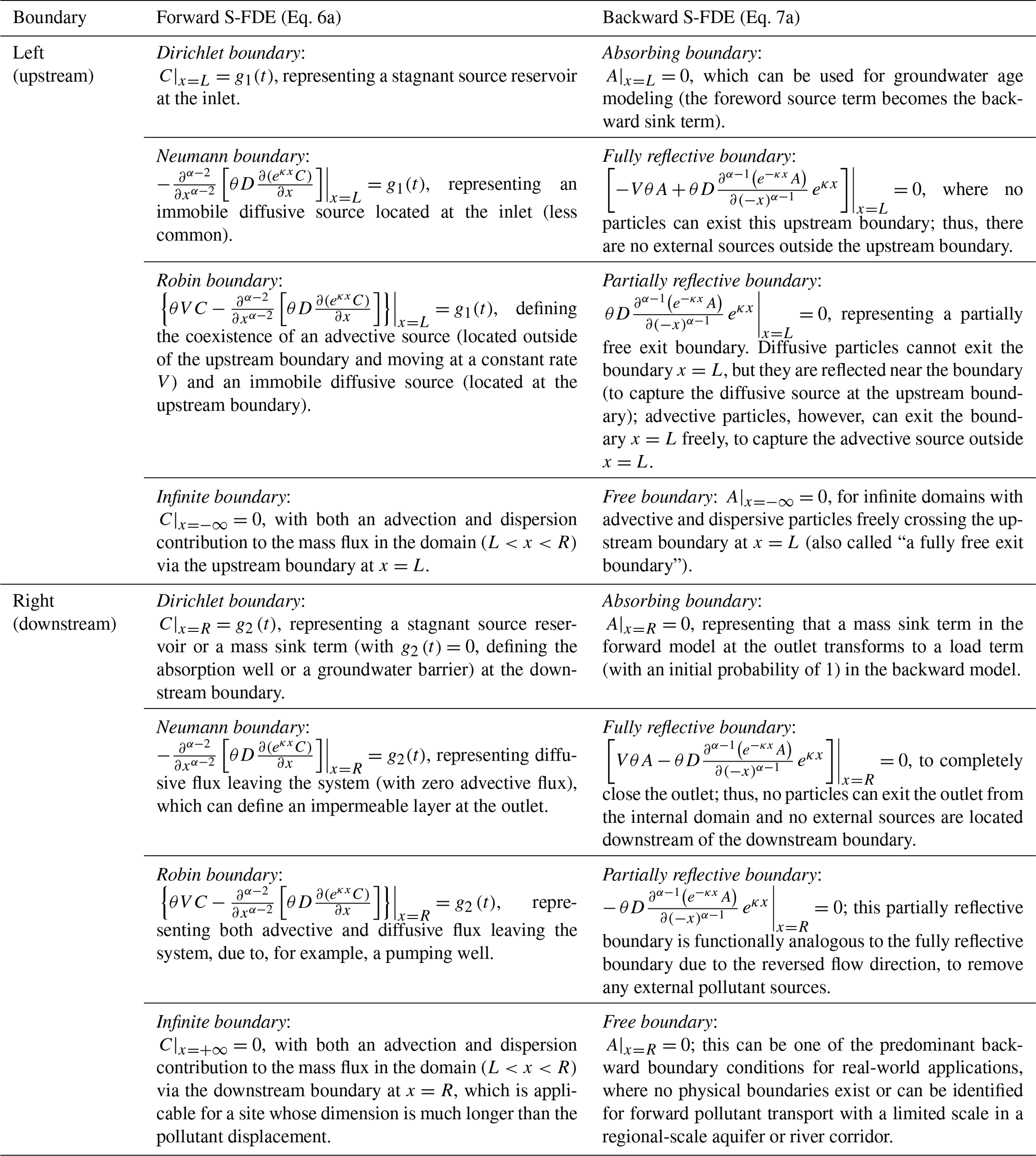
We convert the abovementioned forward-in-time Lagrangian solver to its backward counterpart for adjoint S-FDE (Eq. 4) approximation with three main modifications. First, we reverse vector components of velocity for backward advective displacement of particles during the operational time. Second, we change skewness of the (tempered) α-stable Lévy jumps from positive (to capture downstream mechanical displacement) to negative maximum (to backtrack pollutants located upstream initially). Third, we modify source/sink terms and boundary conditions according to those defined in the adjoint model (Eq. 4) and Table 1. For example, forward sink term (−q_oC in Eq. 1a) becomes the load term $\frac{\partial h}{\partial C}$ in the adjoint model (Eq. 4a), representing the initial probability source in the backward Lagrangian solver. Table 1 details changes and hydrogeologic interpretations of these boundary conditions (value and type) converted from the forward S-FDE to backward counterpart at upstream (inlet) and downstream (outlet) boundaries. In this 1D simplification, we assume forward flow left to right. The Dirichlet, Neumann, Robin, and infinite boundaries in the forward model transform to the absorbing, fully reflective, partially reflective, and free boundaries in the backward model, respectively, to correctly backtrack particle trajectories around boundaries and recover the pollutant release history. For example, the nonzero Dirichlet boundary condition in the forward model (Eq. 1c) converts to an absorbing boundary in the backward model (Eq. 4c), which is expected because the forward source term becomes the sink term in the backward model. In addition, a nonzero Neumann boundary condition in the forward model (Eq. 1d) (representing an immobile diffusive source at the inlet boundary) transforms into a fully reflective boundary condition in the backward model (Eq. 4d) (meaning no external sources outside the upstream boundary), ensuring that no particles exit this upstream boundary (Table 1).

Table 1 Changes in boundary conditions from the 1D forward FDE (Eq. 6a) to its backward model (Eq. 7a).

This backward-in-time Lagrangian solver is computationally more efficient than the standard Eulerian solver because (i) particles in the immobile phase remain motionless, and therefore require no calculations, and (ii) the streamlines can be semi-analytically calculated (LaBolle, 2006) for streamline-projected mechanical dispersion during regional flow subordination.

2.3 Numerical experiments and validation

Here, we check this Lagrangian solver using either simplified cases (1D) or qualitative evaluation due to the lack of other numerical solvers for the 3D adjoint S-FDE (Eq. 4a). The number density of particles exiting the source location, rescaled by velocity, defines the flux-concentration-based BTTP. This method estimates the PDF of each release time (s) for the pollutants identified at the monitoring well at present.

Results of the first numerical experiments are plotted in Fig. 1. For validation, we developed an implicit Eulerian finite difference solver for the 1D adjoint FDE (Eq. 7a), adopting the Grünwald approximation scheme proposed by Meerschaert and Tadjeran (2004) for efficient fractional derivative approximations. The Lagrangian BTTP solutions align with the Eulerian solutions, despite some apparent noise at low BTTPs, arising from the finite number of particles used in the model (Fig. 1). In these experiments, we assumed the backward travel distance of 10 (dimensionless) and a model domain dimension 100 times larger than the backward travel distance. Consequently, we treated the boundaries as effectively infinite and applied the free boundary condition as outlined in Table 1. Our numerical analysis also revealed that varying the time truncation parameter λ impacts the BTTP peak time and the late-time tail. A larger λ delays the BTTP peak time (because a larger λ leads to a longer peak waiting time in the truncated stable density) and narrows the late-time tail of the BTTP (because a larger λ significantly narrows the particle's waiting time PDF by truncating extremely long waiting times) (Fig. 1a, b). When λ is very small (i.e., $\mathit{\lambda }\le {\mathrm{10}}^{-\mathrm{6}}$ T⁻¹, representing an untruncated, standard stable density for the random waiting time), the late-time BTTP tail declines at a rate of $s^{-\mathrm{1}-\mathit{\gamma }}$ (Fig. 1d). In addition, a small and negligible space truncation parameter κ results in an early-time BTTP tail increasing at a rate of s¹, a characteristic stable across various subordination indexes α varying from 1 to 2 (Fig. 1b, d). When all the other parameters remain unchanged, a smaller subordination index α and a larger time index γ accelerates the BTTP peak, because a smaller α engenders a faster-moving plume peak and a larger γ describes weaker retention. Therefore, the BTTP early-time tailing behavior (representing super-diffusion) is governed by α and κ, while the late-time tailing behavior (representing sub-diffusion) is mainly controlled by γ and λ. The BTTP peak is affected by all four of these parameters, reflecting the interplay between super- and sub-diffusive transport. These BTTP features can be critical signals for real-world applications. For example, the BTTP peak time describes the most likely release time of an instantaneous point source, and the BTTP tails control the backward travel time distribution which also defines the groundwater age distribution (see the application in Sect. 3.2) and transient indexes for assessing aquifer vulnerability (Zhang et al., 2018).

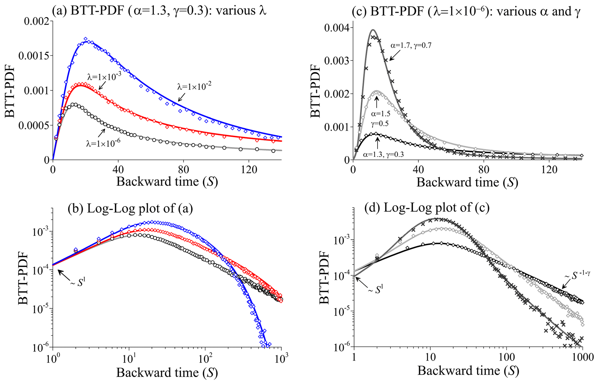
Figure 1 Solver validation 1: Lagrangian solutions (symbols) vs. the Eulerian solutions (lines) for the 1D backward model (Eq. 7a) with various truncation parameters λ (a) and various subordination index α and time index γ (c). The other model parameters that remain unchanged in these cases are as follows: velocity V=1, scaling factor ${\mathit{\sigma }}^{*}=\mathrm{1}$, the spatial truncation parameter $\mathit{\kappa }=\mathrm{1}\times {\mathrm{10}}^{-\mathrm{7}}$, and the backward travel distance L=10. Panels (b) and (d) are the log–log plots of panels (a) and (c), respectively, to show the tailing. Free exit boundary conditions are used in these cases, and parameters are dimensionless here.

The second numerical experiments apply the Lagrangian solver to backtrack particles in nonuniform flow fields (Fig. 2). Two 2D Brownian random hydraulic conductivity (K) fields were first generated using the method developed by Zhang et al. (2019a) (Fig. 2a, c). Particularly, lognormal, random K values were distributed in space using the Fourier filter function. The Hurst parameter in the filter function defines the spatial correlation of K values: a relatively “homogeneous” K field exhibits weak correlation of K (e.g., Fig. 2a), while a “heterogeneous” K field displays strong correlation (e.g., Fig. 2c). Steady-state groundwater flow was then calculated by the United States Geological Survey (USGS) software MODFLOW (Harbaugh, 2005) (shown by the black lines in Fig. 2 and d). Backward particle-tracking plumes were finally obtained by the Lagrangian solver proposed above (shown by the contour maps in Fig. 2b and d). In K-field no. 1, characterized by a relatively “homogeneous” distribution of K, particles originating from different wells move backward at a similar rate, eventually exiting the system upon reaching the upstream boundary (located at x=0 and assumed to be an absorbing boundary in the backward model) (Fig. 2b). These plumes follow local streamline paths, in accordance with the streamline projection method outlined earlier. The transverse expansion of the plume is attributed to molecular diffusion incorporated into particle dynamics. In K-field no. 2, representing a more heterogeneous K field with layered deposits, particles starting in the high-K zone move rapidly and exit the model domain (Fig. 2d). These backward dynamics follow our logical expectations but cannot be independently validated, as far as our knowledge extends, due to the absence of alternative solvers for the vector model (Eq. 4).

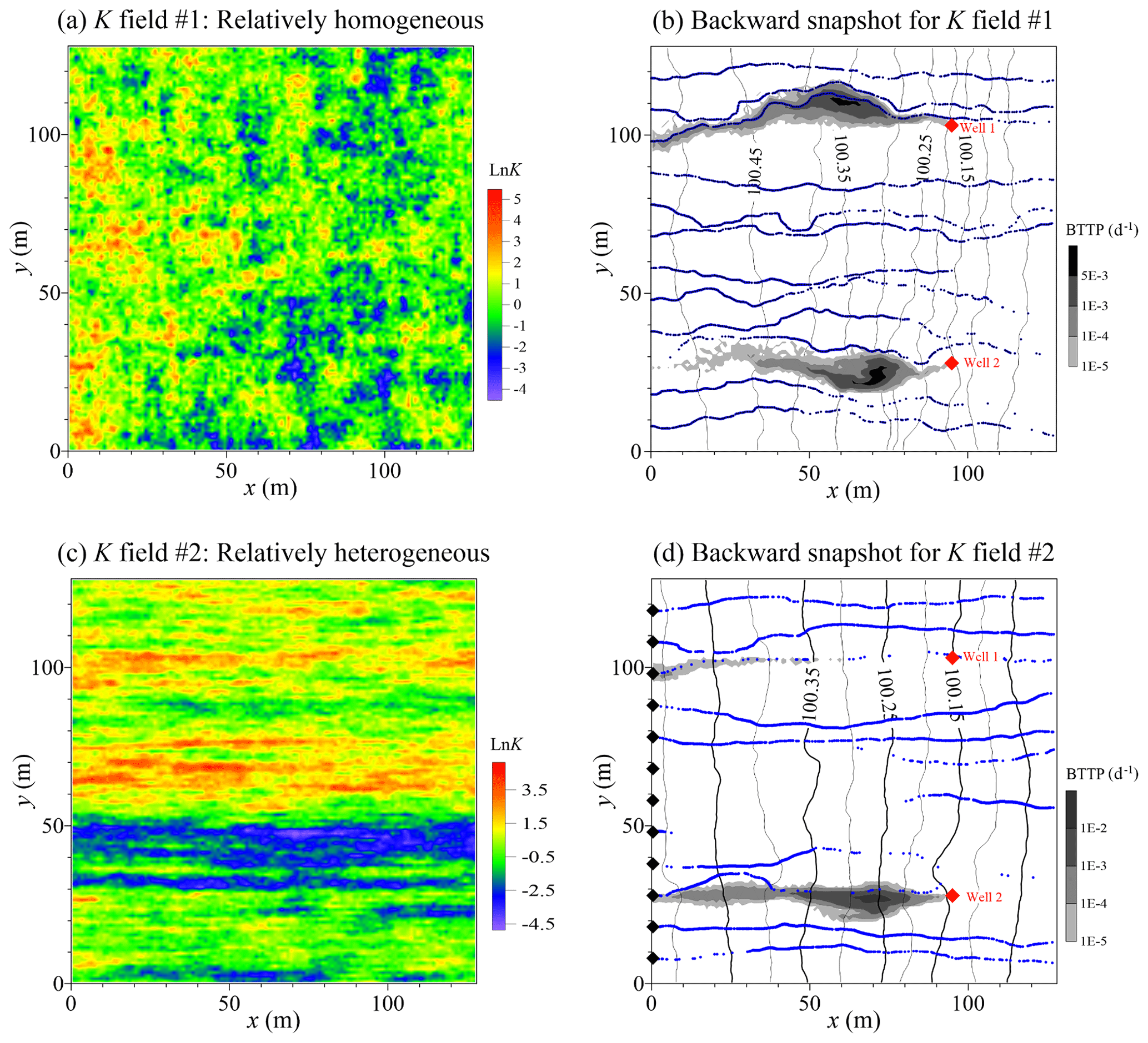
Figure 2 Solver validation 2: two cases of operator fractional Brownian fields are given in panels (a) and (c). The corresponding backward particle-tracking plume using the Lagrangian solvers for K-field no. 1 and no. 2 is plotted in panels (b) and (d), respectively. In panels (b) and (d), black lines represent the hydraulic head calculated by MODFLOW, dotted blue lines denote the streamlines starting from the left boundary shown by the black diamonds in (d), and the red diamonds show the locations of two monitoring wells.

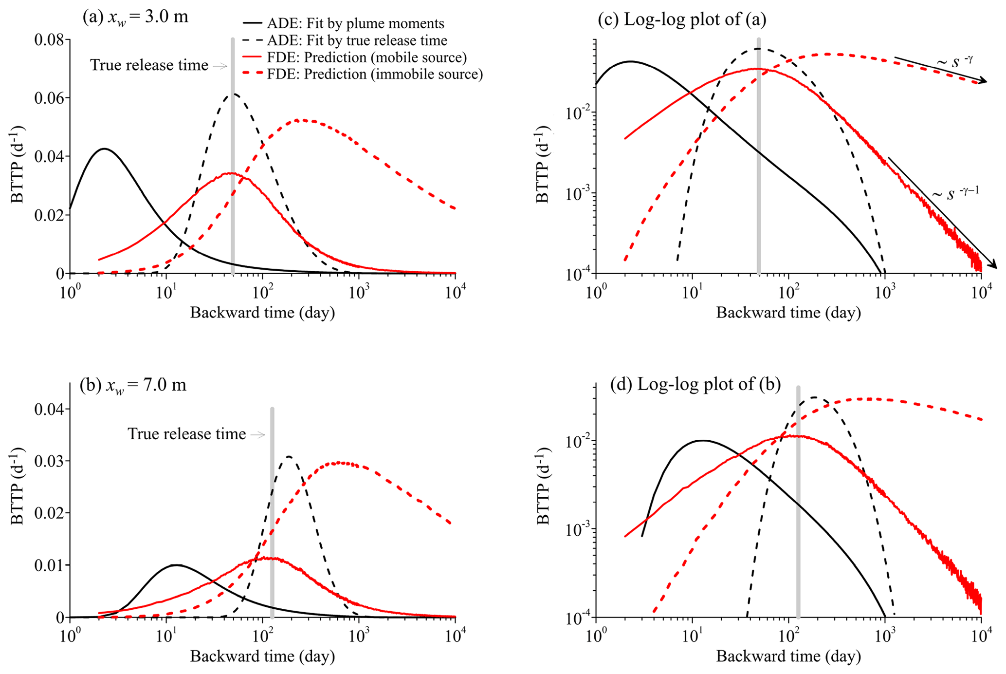
Figure 3 BTTP application 1 – MADE-1 aquifer: the calculated BTTP using the adjoint 1D S-FDE (red lines) and the adjoint 1D ADE (black line) for the observation well located at x_w=3.0 m (a) and x_w=7.0 m (b). Panels (c) and (d) are the log–log plots of panels (a) and (b), respectively, to show the tailing behavior. The vertical gray bar denotes the true release time. The solid red line represents the BTTP for a mobile source, whereas the dashed red line represents the BTTP for an immobile source.

3 Field applications

The adjoint S-FDE model is applied in this section to recover the release history of pollutants in aquifers and rivers and calculate groundwater ages dated by environmental tracers. These surface and subsurface flow systems, characterized by different levels of medium heterogeneity, diverse flow velocity resolutions, boundary conditions, and spatiotemporal scales, serve as a comprehensive test bed to evaluate the real-world applicability of the physical model and numerical solver developed in this study.

3.1 BTTP application case 1: recover release history of pollutants at the MADE site

Natural-gradient tracer tests were conducted at the Macrodispersion Experiment (MADE) site in Columbus, Mississippi, USA (Adams and Gelhar, 1992; Boggs et al., 1992), identifying mixed sub- and super-diffusive pollutant transport in an alluvial aquifer measuring approximately 11 m with respect to thickness and 300 m with respect to length (Bianchi et al., 2016; Yin et al., 2020). Non-Fickian transport at the MADE site has motivated the development of various numerical and stochastic transport models over the last 3 decades (see the review by Zheng et al., 2011), but the BTTP dominated by mixed sub-/super-diffusion has remained uncharted. Here, we calculate its BTTP using the adjoint S-FDE (Eq. 7a), an upscaled model, with a uniform velocity. The 1D backward model is selected because the MADE site transport can be simplified by a 1D process projected into the longitudinal direction, which is a convention upheld by many previous models (Zheng et al., 2011).

The seven parameters in the backward model (Eq. 7a) can be conveniently estimated using mainly literature data. The strong sub-diffusion and super-diffusion observed at the MADE site imply that the two truncation parameters (λ and κ) can be simply neglected, reducing the unknown parameters to 5. The subordination index α is analogous to the spatial index (1.1) estimated by Benson et al. (2001) using the distribution of measured permeability. The time index γ (0.39) and capacity coefficient β (0.082 d^γ−1) were estimated by Zhang (2010) using the decline rate of the observed mobile tracer mass. The velocity V (0.24 m d⁻¹) can be approximated by the mean field velocity, and the scaling factor σ^* is assumed to be 1 m because dispersion at the MADE site was found to be a similar order to V (Benson et al., 2001).

The predicted BTTPs are plotted in Fig. 3. Here, we choose the monitoring well located at the bromide plume's peak (obtained from the MADE-1 bromide tracer test) as the detection location, denoted as x_w (which is defined as the location of the monitoring well detecting the maximum concentration), as this location represents the mass center of the tracer plume. The known contaminant source is situated at the origin (x₀=0). The plume peak during the first (Day 49) and second (Day 126) sampling cycles is located at x_w=3.0 m and 7.0 m, respectively, providing two possible detection locations. These two detection locations lead to the two predicted BTTPs depicted in Fig. 3, after applying the adjoint S-FDE (Eq. 7a) with the seven parameters estimated above.

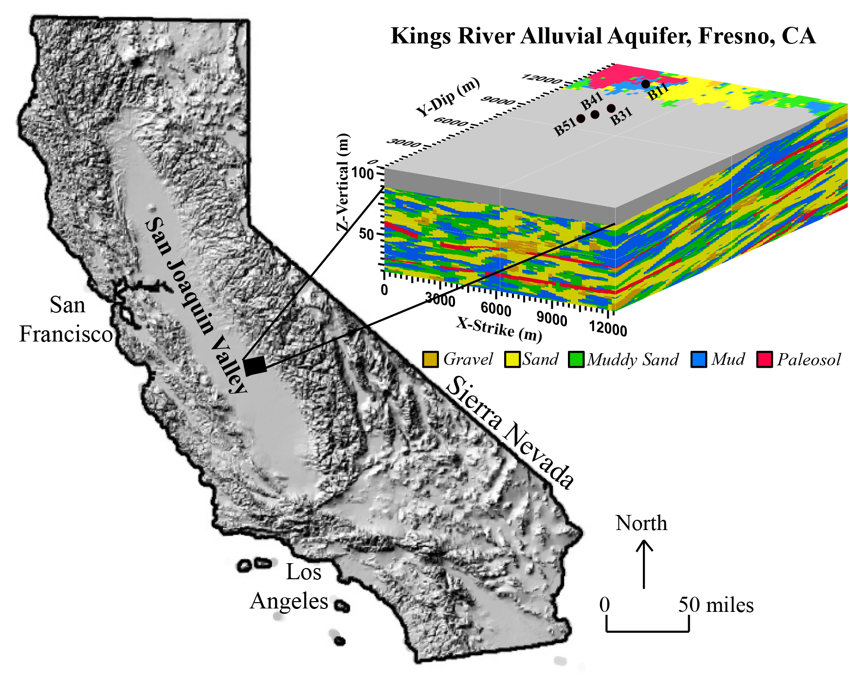
Figure 4 BTTP application 2 – KRAA: location and the multiscale 3D hydrofacies model for the Kings River alluvial aquifer, Fresno County, California, USA.

On the one hand, the model results show that the peak in the flux-concentration-based BTTP well captures the true release time (Fig. 3a, b); on the other hand, the peak in the BTTP based on the concentration profile for “immobile” particles (which remained nearly stationary at the source location during each unit time interval for BTTP calculation) has a higher value and corresponds to a much later time (twice that of the flux-concentration-based BTTP peak), which significantly overestimates the true release time. This discrepancy is explained by the slower movement of the immobile-phase source (than the mobile-phase source) due to strong solute retention, resulting in a more aged release time. For an aqueous-phase observation, the flux-concentration-based BTTP describes the PDF of release times for aqueous-phase (or mobile-phase) sources, while the immobile particles' concentration-based BTTP describes the PDF of release times for absorbed-phase (or immobile-phase) sources. In the MADE-1 tracer test, bromide tracer was initially injected into the upstream well as a mobile source, necessitating the use of the flux-concentration-based BTTP. This demonstrates that the adjoint S-FDE (Eq. 7a) successfully recovers the tracer's release history. In addition, as shown in Fig. 3c, the slope of the late-time BTTP for the immobile-phase sources on a log–log plot (which is −γ) is −1 smaller (i.e., heavier) than that for the mobile-phase sources (which is $-\mathit{\gamma }-\mathrm{1}$), describing the sustained release of immobile pollutant mass at the source location and implying a high degree of uncertainty in the BTTP for the immobile-phase source.

The adjoint ADE is also applied here for comparison. When the same velocity V (0.24 m d⁻¹) and dispersion coefficient D^* (${\mathit{\sigma }}^{*}V=\mathrm{0.24}$ m² d⁻¹) are used, the adjoint ADE significantly underestimates the true release time (not displayed here), as it cannot account for solute retention. Subsequently, we attempted calibration by adjusting V (0.068 m d⁻¹) and D^* (0.68 m² d⁻¹) to match the mean and variance of the observed bromide plumes. However, the resulting BTTP peak still underestimated the true release time by over 1 order of magnitude (shown by the solid black line in Fig. 3). Finally, we directly fitted V (0.026 m d⁻¹, 1 order of magnitude smaller than the mean groundwater velocity) and D^* (0.031 m² d⁻¹) using the true release time for the detection well located at x_w=3.0 m (shown by the dashed black line in Fig. 3a). Nevertheless, this best-fit adjoint ADE overestimated the true release time by >50 % for the detection well at x_w=7.0 m (shown by the dashed black line in Fig. 3b). Therefore, the adjoint ADE with a constant velocity cannot reliably recover the release history of pollutants experiencing strong non-Fickian transport in the MADE aquifer, reaffirming conclusions drawn in previous studies regarding tracer transport at the MADE site using ADE-based models (Zheng et al., 2011).

3.2 BTTP application case 2: groundwater age dating in Kings River alluvial aquifer, California

The vector backward S-FDE (Eq. 4a) is then used to calculate groundwater age distributions for the Kings River alluvial aquifer (KRAA) in Fresno County, California, USA (Fig. 4). The flux-concentration-based BTTP also represents the groundwater age distribution and serves as crucial data for groundwater sustainability assessments (Fogg et al., 1999; Weissmann et al., 2002; Fogg and LaBolle, 2006).

The KRAA system comprises five paleosol-bounded stratigraphic sequences recognized by Weissmann and Fogg (1999). One realization of the 3D hydrofacies model built upon the Markov chain model developed by Weissmann et al. (2004) is shown in Fig. 4, where the hydrofacies model incorporates both the large-scale stratigraphic sequences and the intermediate-scale hydrofacies within each sequence. This 3D Markov chain model was built using hydrofacies distribution data from 11 cores, 132 drillers' logs, and soil survey data. All cores and drillers' logs were integrated as hard conditional data, maximizing the incorporation of observed information into the numerical model. This regional-scale model contains ∼1 million cells, each with dimensions of 200, 200, and 0.5 m in the depositional strike, depositional dip, and vertical directions, respectively, with a total model domain size of 12 600 m × 15 000 m × 100.5 m along these three directions. We calculated steady-state groundwater flow using MODFLOW, applying parameters and boundary conditions described by Weissmann et al. (2004) and Zhang et al. (2018). Specifically, we assigned measured K values to each facies (gravel, sand, muddy sand, mud, and paleosol). The top of the model accounted for a recharge boundary, and the lateral and basal boundaries of the model were general head boundaries to allow inflow and outflow. The modeled hydraulic heads closely matched the measured data (Zhang et al., 2018). We used the resulting fine-resolution velocity field to calculate the BTTP using the adjoint S-FDE (Eq. 4a).

We begin with a parameter sensitivity test using the adjoint S-FDE (Eq. 4). In these backward particle-tracking models, the water table (representing an internal boundary) and the lateral upstream boundary of the model are both set as absorbing boundaries, representing the source locations. The remaining model boundaries are treated as fully reflective boundaries. An effective porosity of 0.33, a value previously determined as the best fit in Weissmann et al. (2004) and Zhang et al. (2018), is applied for these simulations. We consider three cases to explore decreasing super-diffusion and increasing sub-diffusion. Case 1 exhibits strong super-diffusion, characterized by a time index γ=0.80, a capacity coefficient β=0.1 yr^γ−1, a subordination index α=1.40, and a scaling factor ${\mathit{\sigma }}^{*}=\mathrm{0.4}$ m. Case 2 represents an intermediate scenario with γ=0.72, β=0.2 yr^γ−1, α=1.45, and ${\mathit{\sigma }}^{*}=\mathrm{0.3}$ m. Case 3 describes strong sub-diffusion, featuring γ=0.65, β=0.3 yr^γ−1, α=1.50, and ${\mathit{\sigma }}^{*}=\mathrm{0.2}$ m. The subordination truncation parameter (κ) remains the same for all three cases ($\mathit{\kappa }=\mathrm{1.0}\times {\mathrm{10}}^{-\mathrm{5}}$ m⁻¹). The resultant backward particle-tracking snapshots at the backward time s=50 years are plotted in Fig. 5a, b, and c for these three cases. Driven by subordination to regional flow, particles follow streamlines and expand, particularly within high-permeability deposits (due also to molecular diffusion simultaneously along all three axis directions). Case 1 captures rapid backward (i.e., toward upstream) movement of particles due to strong super-diffusion, resulting in most particles reaching the water table within 50 years and then leaving the system, leaving only a few particles behind (Fig. 5a). Contrarily, Case 3 captures the most delayed backward movement due to strong sub-diffusion, resulting in the majority of particles remaining in the aquifer with limited spatial expansion, as depicted in Fig. 5c. This parameter sensitivity test demonstrates the capability of the adjoint S-FDE (Eq. 4) to reasonably interpret non-Fickian dynamics in multidimensional aquifers. In addition, the corresponding BTTP for each case, representing the age distribution for groundwater sampled at the well screen indicated in Fig. 5a (the green rectangle), is plotted in Fig. 5d. Notably, as the adjoint S-FDE transitions from Case 1 to Case 3, characterized by a larger subordination index α and a smaller time index γ, the BTTP shifts towards older ages, with a decreasing peak and an expanding distribution. This illustrates the impact of decreasing super-diffusion and increasing sub-diffusion on groundwater age distributions. This test underscores that key properties of the BTTP, including the mean, peak, and variance of groundwater ages, are sensitive to the two indexes α and γ. In further comparisons, it becomes evident that the classical adjoint ADE fails to capture the early arrivals in the BTTP, primarily due to its inability to account for super-diffusion (figures not shown).

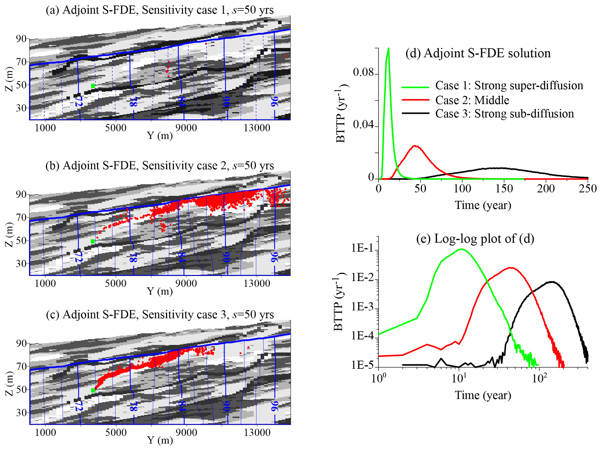
Figure 5 BTTP application 2 – Kings River alluvial aquifer (KRAA): a snapshot (of particle plumes) within the vertical cross-section along the X-strike direction, with a coordinate of X=3700 m shown in the hydrofacies model in Fig. 4. This snapshot was obtained through backward particle tracking over a backward time of s=50 years using the adjoint S-FDE (Eq. 4a) for Case 1 (a), Case 2 (b), and Case 3 (c). The green rectangle in each panel represents the well screen (with a length of 0.5 m) where the groundwater sample was collected. In all cases, 5000 particles were released initially at s=0. Panel (d) shows the corresponding BTTPs for these three cases, and panel (e) is the log–log version of panel (d).

Finally, we compared the adjoint S-FDE solutions with chlorofluorocarbon-11 (CFC-11) ages measured by Burow et al. (1999) from USGS data for the KRAA in 1994. The S-FDE model parameters cannot be predicted using the hydrofacies property-based method proposed by Zhang et al. (2014) for stationary hydrofacies models, due to the nonstationary distribution of hydrofacies in the KRAA. Instead, an alternative approach was employed by fitting the age distribution for groundwater, particularly shallow groundwater, calibrated using environmental tracers such as CFCs. Figure 6a–d present the calculated BTTP for the USGS wells sampled by Burow et al. (1999) (listed in Fig. 4). Both the adjoint S-FDE (Eq. 4a) and the adjoint ADE (Eq. 8a) were first calibrated to fit the measured CFC-11 age of Well B41, following the methodology proposed by Weissmann et al. (2002). Preliminary tests revealed that the simulated CFC-11 age is insensitive to the two truncation parameters, as these parameters primarily affect very early (i.e., <1 d) or very late (i.e., >50 years) times in the BTTP. The velocity field was directly resolved from the MODFLOW solutions of hydraulic head; therefore, velocity was not a fitted parameter. Hence, the adjoint S-FDE (Eq. 4a) has four unknown parameters: the subordination index α and scaling factor σ^*, which control the climbing limb of the BTTP, and the time index γ and capacity coefficient β, which govern the declining limb of the BTTP. The interplay between these two groups of parameters, particularly the two indexes, affects the BTTP peak, as discussed in Sect. 2.3. Here, the primary objective is to determine the best-fit parameters for the two indexes defining super- and sub-diffusion while staying within their established range. To represent strong super-diffusion within a very coarse velocity field, such as a uniform velocity, the subordination index α ($\mathrm{1}<\mathit{\alpha }\le \mathrm{2}$) should approach the lower limit. For example, the MADE-1 site utilized a best-fit α=1.1 with a uniform, upscaled velocity. Conversely, when modeling strong sub-diffusion with a uniform velocity, the time index γ ($\mathrm{0}<\mathit{\gamma }\le \mathrm{1}$) should approach the lower end. For example, the MADE-1 site had a best-fit γ=0.39. With the availability of a fine-resolution velocity field, values of α (or γ) increase and may approach the upper limit of 2 (or 1) if velocity is resolved at the pore scale. The fine-resolution velocity field available for the KRAA allowed for the selection of α and γ close to their upper ends in trial-and-error calibrations, leading to the following best-fit results: the subordination index α=1.90, the scaling factor ${\mathit{\sigma }}^{*}=\mathrm{0.2}$ m⁻¹, the time index γ=0.80, and the capacity coefficient β=0.2 d^γ−1. For the adjoint ADE, the sole fitting parameter is dispersivity, with the best-fit isotropic dispersivity (longitudinal and transverse dispersivities α_L and α_T) of 0.04 m. This same value of isotropic dispersity has also been applied in previous studies modeling KRAA transport processes using ADE-based models by Weissmann et al. (2002, 2004) and Zhang et al. (2018). These studies found that (i) simulation results were insensitive to the value of α_L, as plume spreading is mainly controlled by the hydrofacies-scale heterogeneity captured by the geostatistical model, and (ii) the Lagrangian solver operated more efficiently with isotopic dispersivity.

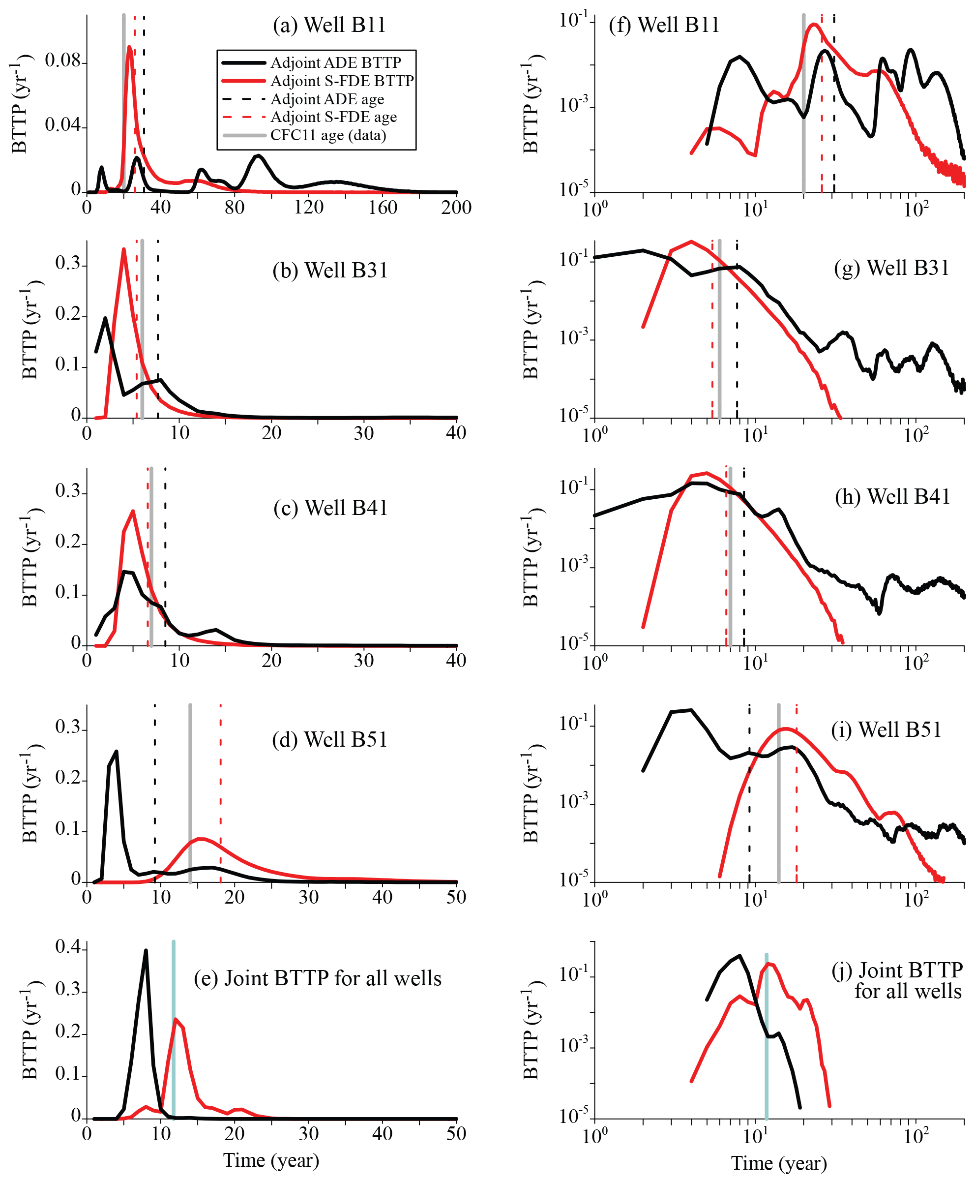
Figure 6 BTTP application 2 – KRF (Kings River alluvial fan): the simulated BTTP using the adjoint S-FDE (red line) and the adjoint ADE (black line) for Well B11 (a), B31 (b), B41 (c), and 51 (d). The right panels are the log–log versions of the respective left panels, to show the tailing. The vertical lines show the CFC-11 age measured in the lab (vertical gray line), estimated by the adjoint S-FDE (dashed red line), and estimated by the adjoint ADE (dashed black line).

The best-fit parameters were then applied to predict the CFC-11 age for the other wells. The CFC-11 age calculated by the adjoint S-FDE matched the observed age better than the adjoint ADE for all wells under consideration. The adjoint ADE produced BTTPs with multiple or secondary peaks, often deviating significantly from the measured CFC-11 ages. In contrast, the adjoint S-FDE typically generated a single BTTP peak closer to the true CFC-11 age, simplifying the interpretation of environmental tracer dating: the apparent age determined from the tracer data usually fell within the range of the 25th to 75th percentiles of the BTTP peak. In addition, Fig. 6e shows the joint BTTP for all wells, representing groundwater recharge times for all four wells simultaneously. The joint BTTP, depicted in a log–log plot (Fig. 6j), exhibited narrower uncertainty compared with individual marginal BTTPs. This reduction in uncertainty results from the availability of concentration data from multiple observation wells. Importantly, this represents the first validated large-scale transport model that combines nonlocal super-/sub-diffusion and local velocities. This application confirms the suitability of the adjoint S-FDE (Eq. 4a) and its Lagrangian solver for capturing BTTP in a 3D, regional-scale, nonstationary alluvial aquifer with a fine-resolution velocity field.

3.3 BTTP application case 3: recover the release time for tracers in Red Cedar River, Michigan

Phanikumar et al. (2007) conducted a study involving the release of fluorescein dye into the Red Cedar River (RCR), a fourth-order stream in Michigan, USA. They then measured breakthrough curves (BTCs) at three locations with travel distances of 1.4, 3.1, and 5.08 km, respectively, to explore the impact of river system retention on dissolved chemicals. The resulting BTCs were fitted by Chakraborty et al. (2009) using a standard, 1D space FDE with a constant velocity. The choice of a 1D model was appropriate due to the relatively straight nature of the river reach. However, as sub-diffusion was found in this stream (Phanikumar et al., 2007) (likely due to open channel retention and/or hyporheic exchange) and the space FDE cannot account for sub-diffusion, we applied the more versatile backward FDE (Eq. 7a). This model encompasses both space and time fractional derivatives and offers a solution to predict the tracer release time.

We first estimated the seven parameters in the 1D adjoint S-FDE (Eq. 7a) using the tracer data. The tracer BTCs measured by Phanikumar et al. (2007) displayed characteristic behaviors, including an exponential mass increase in their ascending limb and rapid mass decrease in their descending limb. These behaviors suggest Fickian diffusion in the operational time (meaning that the subordination index α is close to 2 and the spatial truncation parameter κ is negligible) and weak solute retention (so that the time index γ should be large, and we initially tried γ=0.9). The capacity coefficient β should be small, considering the high mass recovery rate in the field (approximately 90  %) (Phanikumar et al., 2007); hence, we approximated β=0.08 min^1−γ (representing 90 % of mobile mass recovery). The temporal truncation parameter λ (0.034 min⁻¹) was approximated by the reverse of the time interval from the BTC peak to the inflection point of the BTC slope, as shown by Zhang et al. (2022). The mean velocity V (0.0317 km min⁻¹) was estimated by the speed of the BTC peak moving from the first sampling location (L=1.4 km) to the second one (L=3.1 km). The last parameter, dispersion coefficient D^* (σ^*V), was estimated to be 0.00317 km² min⁻¹ by assuming that dispersion is 1 order of magnitude smaller than advection, as solute transport in rivers is usually dominated by advection. These estimations, while inherently uncertain, served to simplify the application of a complex model with seven unknown parameters in the field.

The peak in the predicted flux-concentration-based BTTPs using the 1D adjoint S-FDE (Eq. 7a) captures the true release time for stream gauges located at L=3.1 km (gauge no. 2) and 5.08 km (gauge no. 3) (shown by the solid red line in Fig. 7b and c). However, it slightly underestimates the true release time for gauge no. 1 located at L=1.4 km (Fig. 7a). This discrepancy arises because the velocity was estimated based on transport data for tracers passing gauge no. 1. For comparison, we also employed the adjoint ADE model. When using the same values of V (0.0317 km min⁻¹) and D^*(0.00317 km² min⁻¹), the adjoint ADE model consistently underestimates the true release times for all gauges (illustrate by the solid black line in Fig. 7). Attempts to fit V and D^* for the first gauge to match the true release time for tracers captured at gauge no. 1 still result in the adjoint ADE model underestimating the true release time for tracers captured at gauge nos. 2 and 3. Therefore, the adjoint S-FDE (Eq. 7a) proves to be a more suitable choice than the classical adjoint ADE for recovering pollutant release history in this river with a constant velocity.

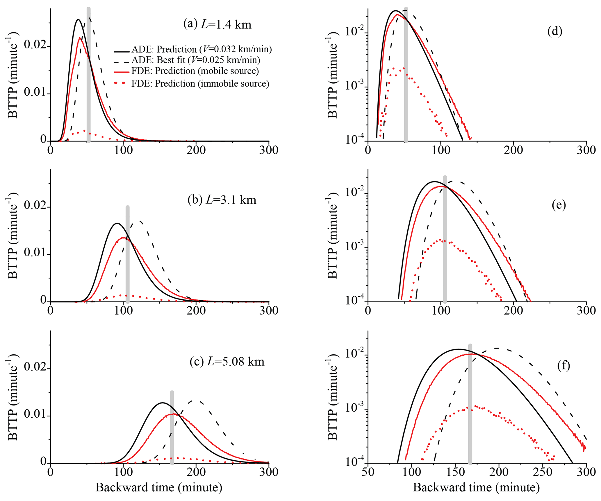
Figure 7 BTTP application 3 – Red Cedar River: the simulated BTTP using the adjoint S-FDE (red lines) and the adjoint ADE (black lines) for the backward travel distance of L=1.4 km (a), 3.1 km (b), and 5.08 km (c). The right panel is the semi-log version of the left panel, to show the tailing. The vertical bar in each panel shows the true release time. In the legend, “FDE: Prediction (mobile source)” represents the predicted BTTP using the adjoint S-FDE for a mobile source, whereas “FDE: Prediction (immobile source)” represents the predicted BTTP for an immobile source.

It is also noteworthy that the BTTP for the immobile-phase sources exhibits a similar peak time and tailing behavior to that of the BTTP for the mobile-phase sources (Fig. 7). This similarity arises from the weak solute retention, as indicated by the large time index γ (resulting in a relatively narrow distribution of the waiting time PDF), the small capacity coefficient β (indicating a smaller fraction of immobile pollutants at equilibrium), and the relatively large time truncation parameter λ (indicating that pollutant transport approaches Fickian scaling once the time exceeds $\frac{\mathrm{1}}{\mathit{\lambda }}\approx \mathrm{32}$ min). This contrasts with the findings for the MADE aquifer discussed in Sect. 3.2, suggesting a more pronounced sub-diffusion in regional-scale alluvial aquifer/aquitard systems compared with rivers.

4 Discussion: extension of field applications and model capabilities

The adjoint subordination approach developed and applied above can also help identify the pollutant source location, a critical factor in pollution source control and water resource management. Furthermore, the backward-in-time vector model (Eq. 4a) has the potential for extension to address more complex transport scenarios. These potential extensions are discussed in the following two subsections.

4.1 Identify pollutant source location using the backward location probability density function

Pollutant source location identification has remained an important topic in hydrology for more than 2 decades, as extensively reviewed by Atmadja and Bagtzoglou (2001), Chadalavada et al. (2011), and Moghaddam et al. (2021). Process-based and statistical models have also been developed over the last 2 years to successfully identify the pollutant source in groundwater and rivers. These models include genetic algorithms combined with groundwater models (Han et al., 2020; Habiyakare et al., 2022) or optimization models (Ayaz et al., 2022), modified export coefficient models integrated with the Soil and Water Assessment Tool (SWAT; Guo et al., 2022), physical/stochastic inverse models (Moghaddam et al., 2021), isotope mixing models (Wiegner et al., 2021; Ren et al., 2021), deep learning models (Kontos et al., 2021; Pan et al., 2021), the model-based backward probability method (Khoshgou and Neyshabouri, 2022), and the null-space Monte Carlo stochastic model (Pollicino et al., 2021), among others.

The adjoint S-FDE (Eq. 4) introduces a new process-based modeling approach to pollutant source location identification by computing a backward location probability (BLP) density function, which is analogous to the normalized resident concentration at a previous time. The peak in this BLP defines the most probable point source location. The term “BLP” represents a standard backtracking scheme, adhering to the established standard procedure for calculating particle-number-density-based PDFs in space. As shown in Sect. 3, where we recovered pollutant release history, the adjoint S-FDE (Eq. 4) offers potential improvements over the classical process-based pollutant source identification models. It can (i) identify the source location for pollutants undergoing non-Fickian diffusion, including super-diffusion, sub-diffusion, their combination, and transitions between non-Fickian and Fickian diffusion; (ii) distinguish the initial source phase; and (iii) accommodate flow fields with varying resolutions. We will validate this hypothesis using real-world data below.

4.1.1 BLP application case 1: SHOAL test site

The adjoint S-FADE (Eq. 4a) was first applied to pinpoint the tracer source at the SHOAL test site in Churchill County, central Nevada, USA. At this site, Reimus et al. (2003) conducted a radial tracer test in a saturated, fractured granite formation. Although the detailed fracture configuration for the granite aquifer was unavailable, researchers categorized the discrete fracture networks (DFNs) into three groups based on fracture aperture (small, medium, and large) using a stochastic approach (Pohll et al., 1999). The ambient groundwater velocity in this setting was estimated to be 0.3–3 m yr⁻¹ (Pohll et al., 1999), which was considered negligible compared with the radial flow generated by the pumping test. During the test, 20.81 kg of bromide with an average concentration of 3.6 g L⁻¹ was injected into a well located 30 m from the extraction well. The measured tracer BTC exhibited power-law tails at both early and late times, although the late-time BTC data were insufficient to determine the full extent of mass decline (depicted by symbols in Fig. 8).

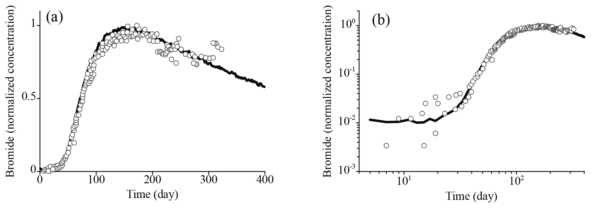
Figure 8 BLP application 1 – SHOAL test site: the measured (symbols) vs. the best-fit (line) bromide breakthrough curve using the vector model S-FDE (Eq. 1a). Panel (b) is the log–log plot of panel (a), to show the BTC tail.

We applied MODFLOW to calculate steady-state flow, approximating the intricate velocity field as radial flow with an average pumping rate of Q=12.4 m³ d⁻¹, consistent with the SHOAL field test. For the sake of upscaling, we simplified the aquifer as “homogeneous,” featuring an average K of $\mathrm{5.78}\times {\mathrm{10}}^{-\mathrm{6}}$ m s⁻¹, falling within the range of bulk hydraulic conductivity, which was $\mathrm{1.48}\times {\mathrm{10}}^{-\mathrm{6}}$–$\mathrm{4.7}\times {\mathrm{10}}^{-\mathrm{5}}$ m s⁻¹, measured by Pohll et al. (1999). We then applied the vector S-FDE (Eq. 1a) with a convergent flow field to match the observed bromide BTC. Figure 8 compares the measured and fitted bromide BTCs. The best-fit parameters in the S-FDE model (Eq. 1a) are as follows: the time index γ=0.44 (without truncation), the capacity coefficient $\mathit{\beta }=\mathrm{0.48}{\mathrm{d}}^{\mathit{\gamma }-\mathrm{1}}$, the subordination index α=1.95, the scalar factor ${\mathit{\sigma }}^{*}=\mathrm{1.0}$, the truncation parameter $\mathit{\kappa }=\mathrm{1.3}\times {\mathrm{10}}^{-\mathrm{3}}$ m⁻¹, and the molecular diffusion coefficient $D^{*}=\mathrm{1.0}\times {\mathrm{10}}^{-\mathrm{5}}$ m² d⁻¹. In Fig. 9, we display the resulting 2D forward-in-time plume snapshots (in the horizontal plane) at both early (t=2 d) and late (t=200 d) times for all phases (mobile, immobile, and total phases). The simulated fractional mass recovery for tracer bromide at the final sampling cycle (t=322 d) reached 20.2 %, which is close to the recovery ratio (18.0 %) estimated by Reimus et al. (2003).

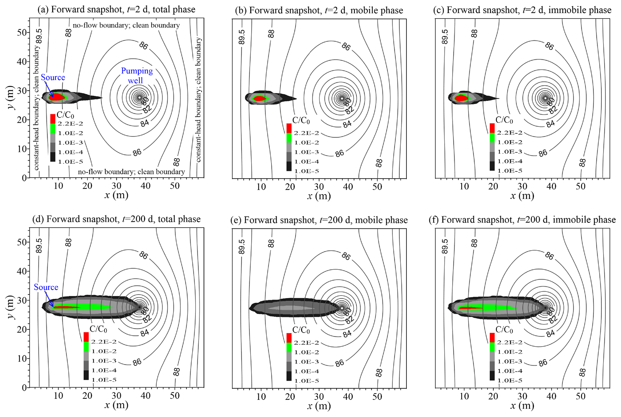
Figure 9 BLP application 1 – SHOAL test site: the modeled forward snapshot for the total phase (a), mobile phase (b), and immobile phase (c) at time t=2 d. Panels (d), (e), and (f) show the snapshot at time t=200 d.

The resulting backward streamlines, computed using the adjoint S-FDE (Eq. 4a), are perpendicular to the groundwater head contour (Fig. 10a), confirming the validity of the concept of subordination to regional flow and our Lagrangian solver. This demonstrates that particles move backward along streamlines, effectively describing backward mechanical dispersion. The simulated BLP is plotted in Fig. 10b, c, and d, where the peak BLP for the mobile-phase source captures the true point source location, considering that the initial point source was within the mobile phase. In contrast, the peak BLP for the immobile-phase source lags behind and is closer to the pumping well due to strong retention. Notably, the divergence in backward flow can disperse particles to different locations, leading to multiple potential sources. Therefore, the adjoint S-FDE (Eq. 4a) and its Lagrangian solver, as developed in Sect. 2, can calculate the BLP for a divergent flow field in a 2D fractured aquifer.

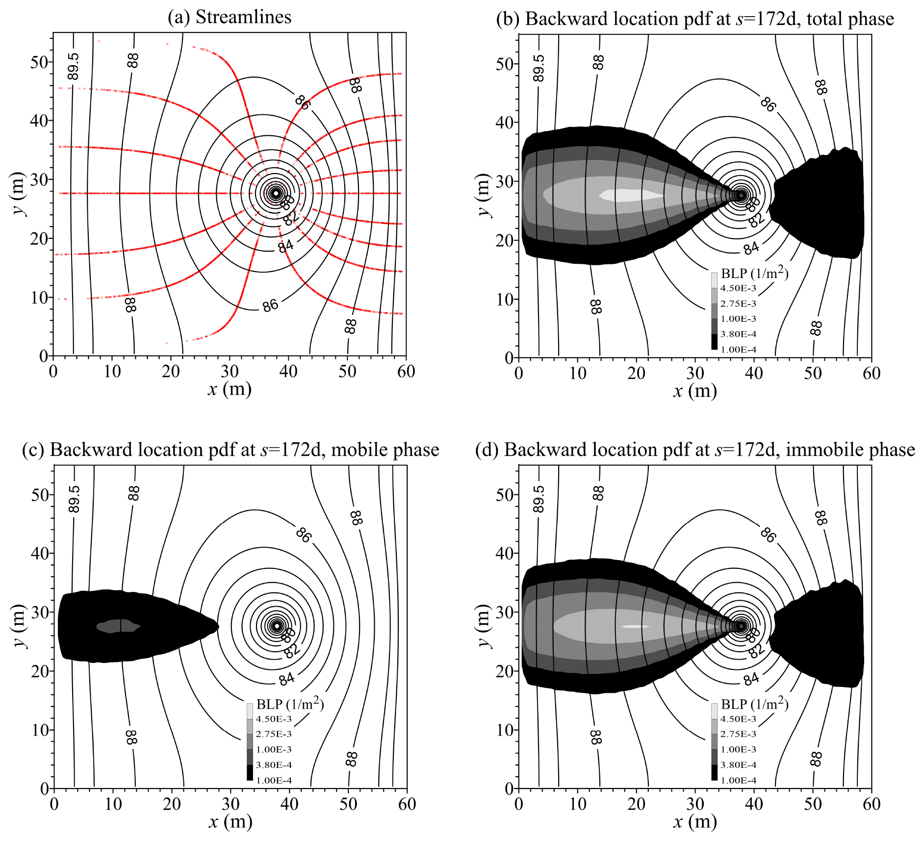
Figure 10 BLP application 1 – SHOAL test site: the modeled backward streamlines starting from the pumping well (a) and the calculated backward location probability density function (BLP) for pollutants located initially in the total phase (b), mobile phase (c), and immobile phase (d). It is noteworthy that there is a low-concentration blob on the east side of the pumping well, due to the divergent flow in the backward model.

4.1.2 BLP application case 2: KRAA

We then applied the adjoint S-FDE (Eq. 4a) to calculate the BLP for non-point pollutant sources within the KRAA system. Figure 11a shows the resulting BLP for Well B51, representing the locations and weights of non-point-source pollutants reaching Well 51 over the past 200 years. This BLP can also serve as the wellhead protection zone under ambient flow conditions, i.e., without pumping. To assess BLP sensitivity to the well depth, we modeled a deeper well named “5b”, located 14.0 m below Well 51, and the resulting BLP is shown in Fig. 11b. The BLP for Well 5b indicates a source center relatively closer to the well than that for Well 51, suggesting the presence of preferential flow paths within the deeper aquifer that the adjoint S-FDE (Eq. 4a) can capture. Figure 11c presents the joint BLP for both wells 51 and 5b, identifying locations where non-point-source pollutants can potentially contaminate both wells. For comparison, we also calculated the BLP using the adjoint ADE, which covers a larger area, particularly near the monitoring well (Fig. 11d). This expansion is likely due to the substantial transverse (vertical) dispersivity (α_T=0.04 m) mentioned in Sect. 3.2. As well depth increases, the center of related pollutant sources shifts further upstream (Fig. 11e). Overall, most of the BLPs calculated by the adjoint S-FDE (Eq. 4a) fall within the BLPs determined by the adjoint ADE (Fig. 11g). This suggests that the adjoint S-FDE (Eq. 4a) tends to reduce the uncertainty in pollutant source identification by emphasizing the impact of dominant flow paths, including preferential flow paths, on regional-scale pollutant transport. Furthermore, this explains why the BLP calculated by the adjoint S-FDE extends slightly further upstream than that of the adjoint ADE, as the adjoint S-FDE captures super-diffusive, large-scale jumps.

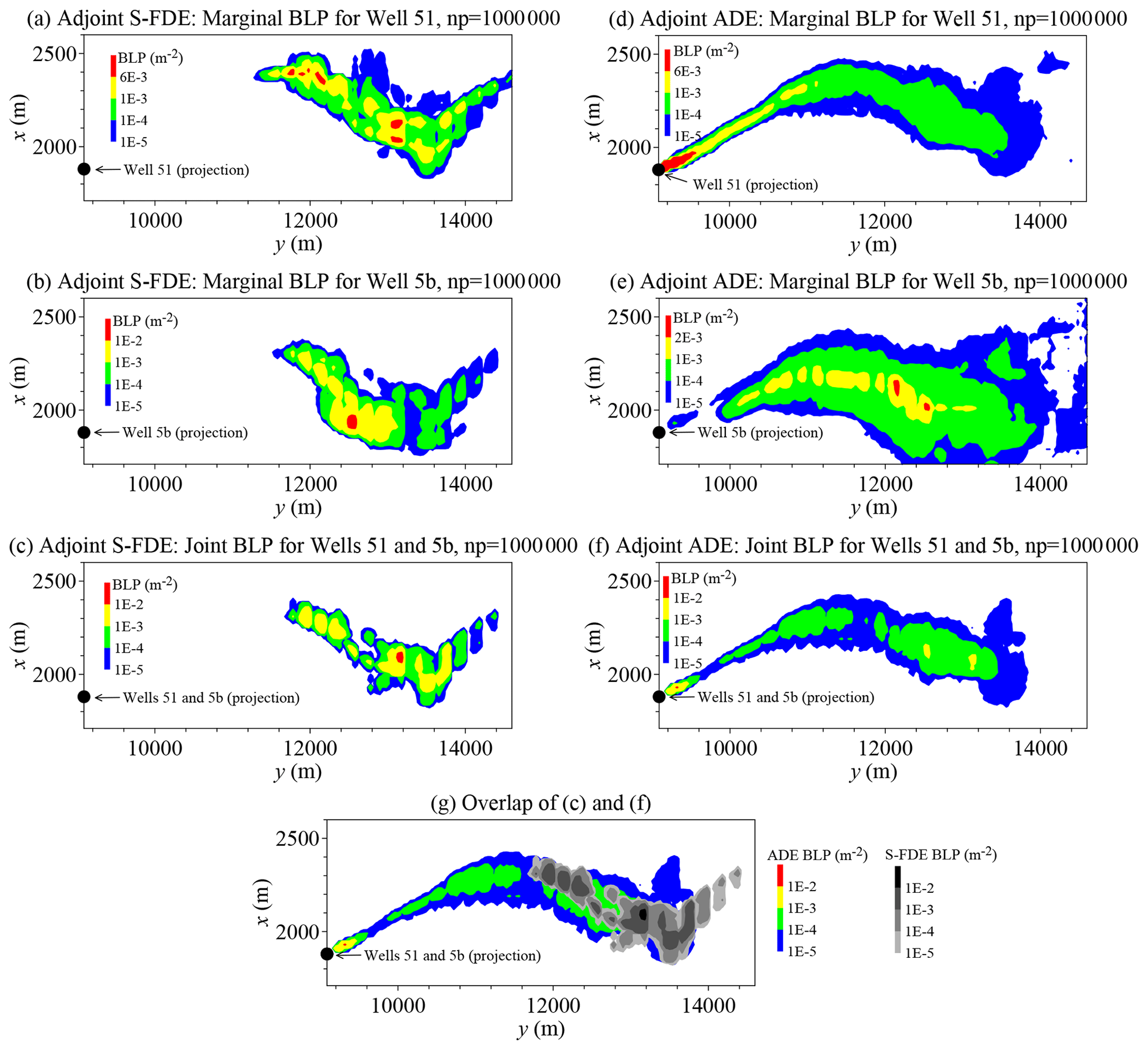
Figure 11 BLP application 2 – KRF: the simulated BLP using the adjoint S-FDE for Well B51 (a), Well B5b (b), and the adjoint BLP for wells B51 and B5b (c). The adjoint ADE results are shown in the right panels. Panel (g) is the overlap of panels (c) and (f). In the legend, “np” denotes the number of particles released in the Lagrangian solver.

4.2 Extension to multi-scaling subordinated model

The backward-in-time vector model (Eq. 4a) has two main limitations. Firstly, it relies on up to seven parameters, the predictability of which remains a challenge. This study conducted preliminary tests for model parameter estimation (in Sects. 3 and 4), and further research on parameter predictability for fractional-derivative models can be found in Zhang et al. (2022). Additional efforts are necessary in future studies to enhance the predictability of FDEs.

Secondly, the subordination index α and scaling factor σ^* in model (Eq. 4a) are limited to constant values, whereas pollutant plumes in natural geological media may exhibit nonuniform, super-diffusive spreading rates. As a preliminary test, we propose the following multi-scaling subordination model as a possible extension of (Eq. 4a), incorporating the multi-scaling fractional derivative concept proposed by Meerschaert et al. (2001):

$$\begin{array}{}\text{(9)}& \begin{array}{rl}& b{\displaystyle \frac{\partial \left(\mathit{\theta }A\right)}{\partial s}}+\mathit{\beta }{\displaystyle \frac{{\partial }^{\mathit{\gamma },\mathit{\lambda }}\left(\mathit{\theta }A\right)}{\partial s^{\mathit{\gamma },\mathit{\lambda }}}}={\mathrm{\nabla }}_{\mathit{V}}\left(\mathit{\theta }A\right)-\mathit{\theta }{\left({\mathrm{\nabla }}_{\overleftarrow{V}}\right)}_{M\left(\overleftarrow{V}\right)}^{\mathbf{H}(\overleftarrow{V}{)}^{-\mathrm{1}}}A\\ & -\left(q_{\mathrm{I}}+\mathit{\theta }r\right)A+{\displaystyle \frac{\partial h}{\partial C}},\end{array}\end{array}$$

where $M\left(\overleftarrow{V}\right)$ denotes the mixing measure that defines the (rescaled) probability of particle movement in each direction of the vector velocity $\overleftarrow{V}$, and $\mathbf{H}(\overleftarrow{V}{)}^{-\mathrm{1}}$ represents the inverse of the scaling matrix that defines the subordination index (with tempering) along the water flow direction of $\overleftarrow{V}$. When $M\left(\overleftarrow{V}\right)$ remains constant (i.e., reduces to the constant σ^*) and the matrix $\mathbf{H}(\overleftarrow{V}{)}^{-\mathrm{1}}$ also reduces to a constant $\stackrel{\mathrm{‾}}{\mathit{\alpha }}$ (with the truncation parameter κ) in all directions, the multi-scaling adjoint S-FDE (Eq. 9) reduces to the unique-scaling model (Eq. 4a).

The general model (Eq. 9) accommodates direction-dependent scaling rates, enabling the capture of multidimensional transport in complex media like regional-scale fractured systems. This function resembles the multi-scaling adjoint fractional-derivative model derived by Zhang (2022):

$$\begin{array}{}\text{(10)}& \begin{array}{rl}& b{\displaystyle \frac{\partial \left(\mathit{\theta }A\right)}{\partial s}}+\mathit{\beta }{\displaystyle \frac{{\partial }^{\mathit{\gamma },\mathit{\lambda }}\left(\mathit{\theta }A\right)}{\partial s^{\mathit{\gamma },\mathit{\lambda }}}}=\mathrm{\nabla }\cdot \left(\mathit{\theta }\mathit{V}A\right)-\mathit{\theta }D{\mathrm{\nabla }}_{\stackrel{\mathrm{‾}}{M}\left(\mathrm{d}\mathit{\theta }\right)}^{{\stackrel{\mathrm{‾}}{\mathbf{H}}}^{-\mathrm{1}}}A\\ & -\left(q_{\mathrm{I}}+\mathit{\theta }r\right)A+{\displaystyle \frac{\partial h}{\partial C}},\end{array}\end{array}$$

where the mixing measure $\stackrel{\mathrm{‾}}{M}\left(\mathrm{d}\mathit{\theta }\right)=M\left(\mathrm{d}\mathit{\theta }+\mathit{\pi }\right)$ is reversed for each discrete angle dθ for backward particle jumps, and the corresponding scaling matrix $\stackrel{\mathrm{‾}}{\mathbf{H}}$ is also reversed by π along each eigenvector direction. The multi-scaling adjoint FDE (Eq. 10) is applicable to a space-dependent velocity vector V, where the spreading angles and weights in the mixing measure $\stackrel{\mathrm{‾}}{M}\left(\mathrm{d}\mathit{\theta }\right)$ can change with velocity. The computational burden of model (Eq. 10), however, increases with higher flow resolution. This is because particle displacement during each jump event must be divided into multiple sections and then projected into an adjacent streamline deviating with the angle of dθ+π from the starting velocity vector. This process, known as the streamline projection method with nonzero projection angles, was demonstrated by Zhang (2022). It can result in a prohibitive computational burden for a regional-scale aquifer with complex flow, such as the KRAA site. To overcome this challenge, the multi-scaling adjoint S-FDE (Eq. 9) employs the streamline-orientation approach, eliminating the need for a deviation angle of dθ+π because mechanical dispersion follows the streamlines.

Here, we first validate the Lagrangian solution of model (Eq. 9) using a straightforward scenario with an existing alternative solution. Figure 12c shows the Lagrangian solution of the multi-scaling S-FDE, based on the mixing measure (with divergent flow) and the scaling matrix (with a constant index) depicted in Fig. 12b. This scenario characterizes pollutant transport in a DFN with multiple orientations (Fig. 12a). The Lagrangian solution matches well with Nolan's (1998) multivariate stable distribution (Fig. 12d).

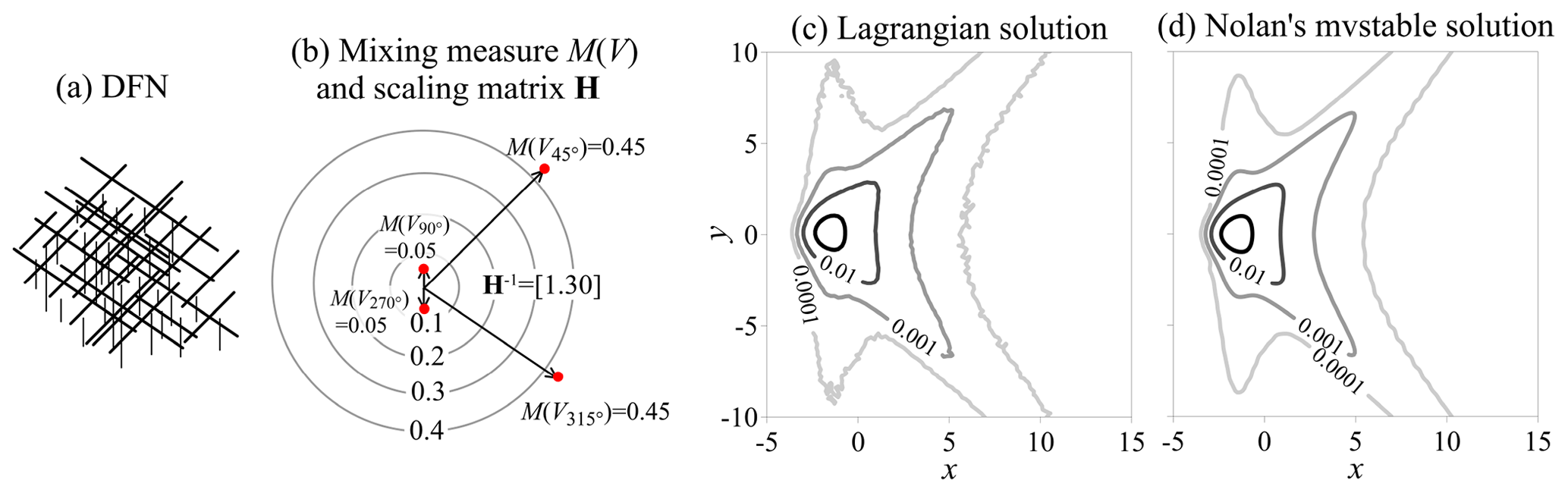
Figure 12 Solver validation: panel (a) shows the schematic diagram of a 2D discrete fracture network, panel (b) is the polar plot of the discrete mixing measure and the scaling matrix, panel (c) is the Lagrangian solution of the multi-scaling S-FDE, and panel (d) is Nolan's (1998) multivariate stable distribution.

Next, we apply model (Eq. 9) to track pollutant transport in a 2D DFN. Figure 13a shows the ensemble average of plume snapshots at time t=4.6 years obtained from Monte Carlo simulations of pollutant transport in 100 DFNs generated by Reeves et al. (2008). These DFNs exhibit multiple orientations, leading to plume movement in various directions. The best-fit solution using the forward-in-time multi-scaling S-FDE is shown in Fig. 13c, effectively capturing plume fingering attributed to super-diffusion along fractures. For comparison, we also apply the multi-scaling FDE proposed by Zhang (2022) to capture the plume snapshot (Fig. 13b), which closely resembles the multi-scaling S-FDE results. These best-fit parameters are then applied to predict plume snapshots at two subsequent time points. It is noteworthy that the multi-scaling S-FDE slightly outperforms the multi-scaling FDE in capturing the plume's center density and rear edge, as evidenced by Fig. 13f vs. Fig. 13g and Fig. 13j vs. Fig. 13k, respectively. The peak in the corresponding BLP calculated by the multi-scaling adjoint S-FDE (Eq. 9) (where reflective boundary conditions are used for all boundaries due to the absence of pollutant recharge from outside) can capture the true point source location. Notably, the plume center appears to remain relatively stationary downstream, due to strong matrix diffusion effects. Additional details regarding model parameter estimation for the DFNs can be found in Zhang (2022). This application shows that the multi-scaling adjoint S-FDE (Eq. 9) can conveniently identify the pollutant source location in DFNs characterized by a uniform, upscaling velocity vector.

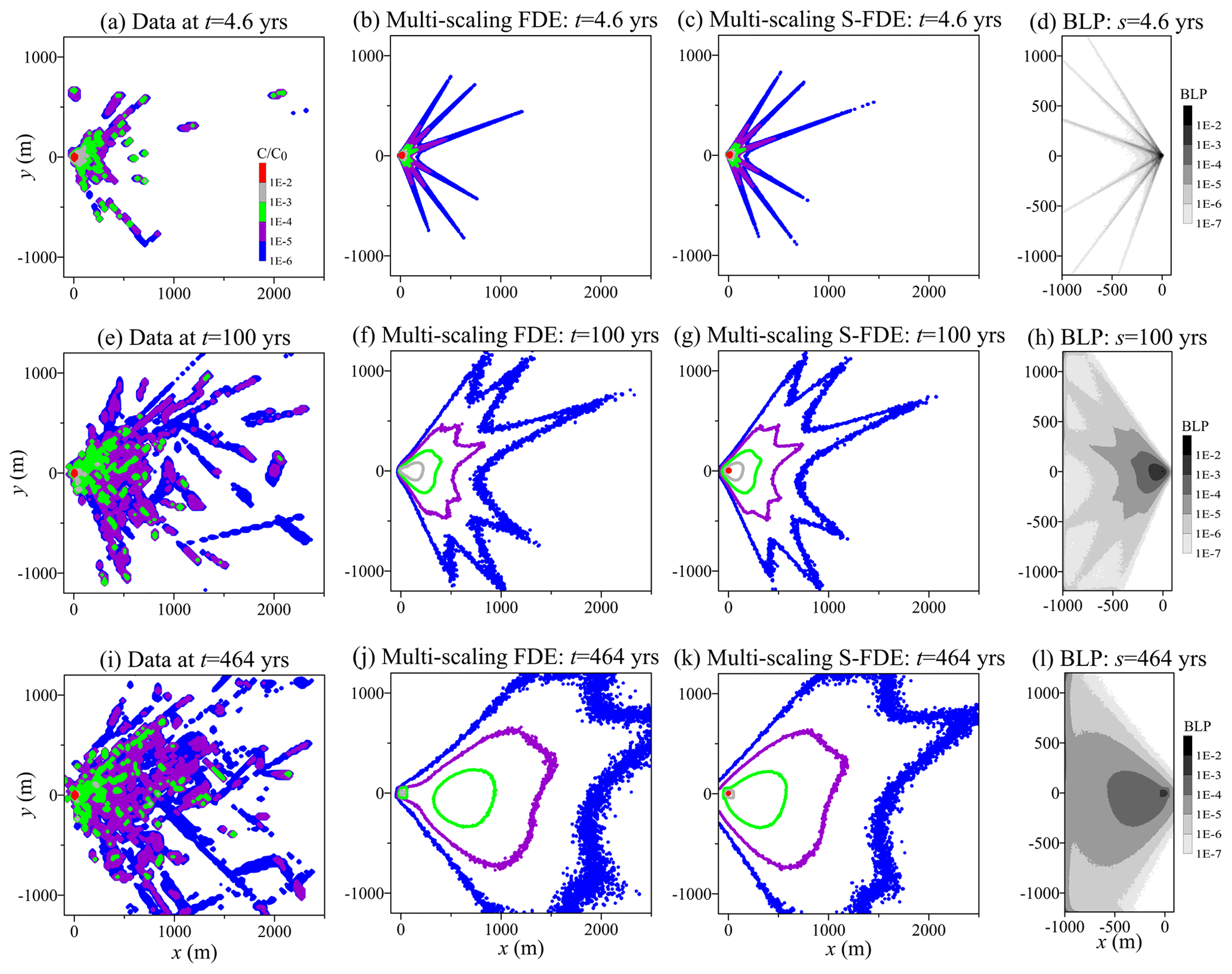
Figure 13 Application of the multi-scaling S-FDE in DFNs: panel (a) shows the average plume snapshot at time t=4.6 years from Monte Carlos simulations of pollutant transport in DFNs (Reeves et al., 2008); panels (b) and (c) are the best-fit solution using the multi-scaling FDE and multi-scaling S-FDE, respectively; panel (d) shows the resultant BLP using the multi-scaling S-FDE; panels (e)–(h) show the result at a later time of t=100 years; and panels (i)–(l) show the result at a later time of t=464 years. Note that the model solutions in the middle and bottom rows are prediction results using parameters fitted in the top row.

5 Conclusions

To reliably track pollutants in natural water flow systems, this study derived the adjoint of the time fractional nonlocal transport model subordinated to regional flow, developed a complete Lagrangian solver, and then applied this new approach to trace pollutants experiencing non-Fickian transport in surface water and groundwater with differing velocity resolutions. Through mathematical analysis and practical hydrologic applications, four key conclusions have emerged.

First, the adjoint subordination approach yielded an adjoint S-FDE model for quantifying backward probabilities, which takes subordination to the reversed regional flow, converts the forward-in-time boundary conditions, and inverts the tempered α-stable density for mechanical dispersion. The resulting backward-in-time boundary conditions can either capture external pollutant sources using the absorbing/free boundary or exclude them with the fully reflective boundary, both of which were tested in applications. The adjoint α-stable density, with tempering, reverses skewness to describe backward, super-diffusive particle displacements along preferential flow paths, which is combined with the self-adjoint time fractional derivative term in the model to capture a broad spectrum of non-Fickian transport dynamics. In addition, the corresponding Lagrangian solver is computationally efficient, as it can simply reverse streamlines to track the backward super-diffusive mechanical dispersion of particles.

Second, in real-world applications, the adjoint S-FDE reliably tracked pollutants in surface water and groundwater across various velocity resolutions. The model successfully recovered pollutant release history and identified pollutant source location(s) in systems characterized by uniform velocity, nonuniform flow fields (i.e., divergent/convergent flow), and fine-resolution velocities in a nonstationary, regional-scale alluvial aquifer. These scenarios often exhibited non-Fickian dynamics, especially sub-diffusion, influenced by solute retention, hyporheic exchange, or matrix diffusion. In such cases, the adjoint S-FDE outperformed the classical ADE-based backward models with respect to calculating BTTP and BLP.

Third, caution regarding the pollutant source phase is needed when backtracking pollutants in natural geologic media. For example, in alluvial aquifers characterized by strong sub-diffusion due to typically abundant aquitard materials, the mobile-phase pollutant source may exhibit a significantly shorter release time and present an apparently further source location compared with the immobile-phase source. However, for large-scale transport in rivers with weak solute retention, the distinction between mobile and immobile pollutant source phases may be less significant. While many field tracer tests (including those revisited in this study) usually involve a mobile initial phase, real-world applications may also encompass immobile pollutant sources (such as dense non-aqueous phase liquid, DNAPL), where the method proposed in this study can be applied.

Fourth, field applications of the adjoint S-FDE face challenges related to the predictability of model parameters, and the model itself may require extensions to handle more complex transport dynamics. This study offered basic parameter estimations based on field measurements, but further research is necessary to establish a quantitative connection between model parameters and media/pollutant properties. In addition, the multi-scaling adjoint S-FDE presents an opportunity to expand upon the unique-scaling adjoint S-FDE and streamline the multi-scaling adjoint FDE for backtracking pollutants in fractured media.

Appendix A: Derivation of the backward model (Eq. 4)

This appendix derives the backward model for the S-FDE (1). Here, we first change the position of the state sensitivity ϕ and the adjoint sate A in the first four terms of Eq. (3) shown in Sect. 2.1.1. For example, the first term in Eq. (3), denoted as I₁, can be rearranged using integration by parts, as follows:

$$\begin{array}{}\text{(A1)}& \begin{array}{rl}{I}_{\mathrm{1}}& ={\int }_{\mathrm{\Omega }}\left[{\int }_{\mathrm{0}}^{T}Ab{\displaystyle \frac{\partial \left(\mathit{\theta }\mathit{\varphi }\right)}{\partial t}}\mathrm{d}t\right]\mathrm{d}\mathrm{\Omega }={\int }_{\mathrm{\Omega }}\left\{\left[Ab\mathit{\theta }\mathit{\varphi }\right]{\mathrm{|}}_{t=\mathrm{0}}^{t=T}\right.\\ & \left.-{\int }_{\mathrm{0}}^T\mathit{\theta }\mathit{\varphi }b{\displaystyle \frac{\partial A}{\partial t}}\mathrm{d}t\right\}\mathrm{d}\mathrm{\Omega }.\end{array}\end{array}$$

The second term in Eq. (3) contains the time fractional derivative and can be rearranged using the fractional-order integration by parts (which does not involve vector field flux through a closed surface), as shown in Zhang (2022):

$$\begin{array}{}\text{(A2)}& \begin{array}{rl}{I}_{\mathrm{2}}& ={\int }_{\mathrm{\Omega }}\left[{\int }_{\mathrm{0}}^{T}A\mathit{\beta }{\displaystyle \frac{{\partial }^{\mathit{\gamma },\mathit{\lambda }}\left(\mathit{\theta }\mathit{\varphi }\right)}{\partial t^{\mathit{\gamma },\mathit{\lambda }}}}\mathrm{d}t\right]\mathrm{d}\mathrm{\Omega }\\ & ={\int }_{\mathrm{\Omega }}\left\{A{\mathrm{|}}_{t=T}\mathit{\beta }{I}_{+}^{\mathrm{1}-\mathit{\gamma },\mathit{\lambda }}\left(\mathit{\theta }\mathit{\varphi }\right){\mathrm{|}}_{t=T}-\left[\mathit{\theta }\mathit{\varphi }\right]{\mathrm{|}}_{t=\mathrm{0}}\mathit{\beta }\right.\\ & \left.I_{-}^{\mathrm{1}-\mathit{\gamma },\mathit{\lambda }}\left(A\right){\mathrm{|}}_{t=\mathrm{0}}+{\int }_{\mathrm{0}}^T\mathit{\theta }\mathit{\varphi }\mathit{\beta }{\displaystyle \frac{{\partial }^{\mathit{\gamma },\mathit{\lambda }}A}{\partial (-t{)}^{\mathit{\gamma },\mathit{\lambda }}}}\mathrm{d}t\right\}\mathrm{d}\mathrm{\Omega },\end{array}\end{array}$$

where the symbol $I_{+}^{\mathrm{1}-\mathit{\gamma },\mathit{\lambda }}\left(f\right)$ denotes the positive fractional integral of order 1−γ: $I_{+}^{\mathrm{1}-\mathit{\gamma },\mathit{\lambda }}\left(f\right)=e^{-\mathit{\lambda }T}{\int }_{\mathrm{0}}^{T}f{e}^{\mathit{\lambda }t}\frac{{\left(T-t\right)}^{-\mathit{\gamma }}}{\mathrm{\Gamma }\left(\mathrm{1}-\mathit{\gamma }\right)}\mathrm{d}t$, the symbol $I_{-}^{\mathrm{1}-\mathit{\gamma },\mathit{\lambda }}\left(f\right)=e^{\mathit{\lambda }T}{\int }_{\mathrm{0}}^{T}f{e}^{-\mathit{\lambda }t}\frac{t^{-\mathit{\gamma }}}{\mathrm{\Gamma }\left(\mathrm{1}-\mathit{\gamma }\right)}\mathrm{d}t$ denotes the negative fractional integral of order 1−γ, and Γ(⋅) is the gamma function.

The third term in Eq. (3), which describes the net advective flux, can be rearranged using the integer-order integration by parts, as follows:

$$\begin{array}{}\text{(A3)}& \begin{array}{rl}{I}_{\mathrm{3}}& ={\int }_{\mathrm{0}}^T\left\{{\int }_{\mathrm{\Omega }}\mathrm{\nabla }\cdot \left[A\mathit{\theta }V\mathit{\varphi }\right]\mathrm{d}\mathrm{\Omega }-{\int }_{\mathrm{\Omega }}\mathit{\theta }V\mathit{\varphi }\mathrm{\nabla }A\mathrm{d}\mathrm{\Omega }\right\}\mathrm{d}t\\ & ={\int }_{\mathrm{0}}^T\left\{{\oint }_{\mathit{\xi }}\left[A\mathit{\theta }V\mathit{\varphi }\right]\cdot \mathit{n}\mathrm{d}\mathit{\xi }-{\int }_{\mathrm{\Omega }}\mathit{\theta }V\mathit{\varphi }\mathrm{\nabla }A\mathrm{d}\mathrm{\Omega }\right\}\mathrm{d}t.\end{array}\end{array}$$

Here, in the second equality, the Gauss divergence theorem is used: ${\int }_{\mathrm{\Omega }}\mathrm{\nabla }\cdot f\mathrm{d}\mathrm{\Omega }={\oint }_{\mathit{\xi }}f\cdot \mathit{n}\mathrm{d}\mathit{\xi }$, where n is the outward normal direction on the boundary ξ. Equations (A1)–(A3) are the same as those shown in Zhang (2022), which is expected as the same time fractional derivative term was used in these FDEs.

The fourth term in Eq. (3) contains the subordination operator and can be rearranged using the integration by parts twice, as shown in Zhang (2022):

$$\begin{array}{}\text{(A4)}& \begin{array}{rl}{I}_{\mathrm{4}}& ={\int }_{\mathrm{0}}^T\left[{\int }_{\mathrm{\Omega }}A{\mathit{\sigma }}^{*}{\left({\mathrm{\nabla }}_{\mathit{V}}\right)}^{\mathit{\alpha },\mathit{\kappa }}\left(\mathit{\theta }\mathit{\varphi }\right)\mathrm{d}\mathrm{\Omega }\right]\mathrm{d}t\\ & ={\int }_{\mathrm{0}}^T\left\{{\oint }_{\mathit{\xi }}{\mathit{\sigma }}^{*}\left[A{I}_{+}^{\mathrm{2}-\mathit{\alpha },\mathit{\kappa }}\left({\mathrm{\nabla }}_{\mathit{V}}\left(\mathit{\theta }\mathit{\varphi }\right)\right)\right]\cdot \mathit{n}\mathrm{d}\mathit{\xi }\right.\\ & \left.+{\oint }_{\mathit{\xi }}{\mathit{\sigma }}^{*}\left[{\mathrm{\nabla }}_{\mathit{V}}\left(\mathit{\theta }\mathit{\varphi }\right)I_{-}^{\mathrm{2}-\mathit{\alpha },\mathit{\kappa }}\left(A\right)\right]\cdot \mathit{n}\mathrm{d}\mathit{\xi }\right\}\mathrm{d}t\\ & +{\int }_{\mathrm{0}}^T\left\{{\oint }_{\mathit{\xi }}{\mathit{\sigma }}^{*}\left[\mathit{\theta }\mathit{\varphi }{\left({\mathrm{\nabla }}_{\mathit{V}}\right)}^{\stackrel{\mathrm{‾}}{\mathit{\alpha }-\mathrm{1}},k}\left(A\right)\right]\cdot \mathit{n}\mathrm{d}\mathit{\xi }\right\}\mathrm{d}t\\ & -{\int }_{\mathrm{0}}^T\left\{{\int }_{\mathrm{\Omega }}{\mathit{\sigma }}^{*}\mathit{\theta }\mathit{\varphi }{\left({\mathrm{\nabla }}_{\overleftarrow{V}}\right)}^{\stackrel{\mathrm{‾}}{\mathit{\alpha }},k}\left(A\right)\mathrm{d}\mathrm{\Omega }\right\}\mathrm{d}t.\end{array}\end{array}$$

Here, the operator ${\left({\mathrm{\nabla }}_{\overleftarrow{V}}\right)}^{\stackrel{\mathrm{‾}}{\mathit{\alpha }},k}$ denotes subordination to the reversed flow field ($\overleftarrow{V})$ where the tempered stable density (with order α) has the maximum possible negative skewness ${\mathit{\beta }}^{*}=-\mathrm{1}$, meaning that fast displacements are from downstream to upstream (for backward tracking).

Neupauer and Wilson (2001) showed that the adjoint state A is a measure of the change in concentration for a unit change in source mass M₀. In sensitivity analysis, the marginal sensitivity of a performance measure A with respect to M₀ is as follows (Neupauer and Wilson, 2001):

$$\begin{array}{}\text{(A5)}& {\displaystyle \frac{\mathrm{d}P}{\mathrm{d}{M}_{\mathrm{0}}}}={\int }_{\mathrm{0}}^T{\int }_{\mathrm{\Omega }}\left[{\displaystyle \frac{\partial h\left(M_{\mathrm{0}},C\right)}{\partial C}}\mathit{\varphi }\right]\mathrm{d}\mathrm{\Omega }\mathrm{d}t,\end{array}$$

where h(M₀,C) is a functional of the state of the system. Inserting I₁–I₄, expressed by Eqs. (A1)–(A4), into the inner product Eq. (3) and then subtracting this updated Eq. (3) from the marginal sensitivity Eq. (A5), we obtain the following:

$$\begin{array}{}\text{(A6)}& \begin{array}{rl}& {\displaystyle \frac{\mathrm{d}P}{\mathrm{d}{M}_{\mathrm{0}}}}={\int }_{\mathrm{\Omega }}{\int }_{\mathrm{0}}^T\mathit{\varphi }\left\{{\displaystyle \frac{\partial h}{\partial C}}+b\mathit{\theta }{\displaystyle \frac{\partial A}{\partial t}}-\mathit{\beta }\mathit{\theta }{\displaystyle \frac{{\partial }^{\mathit{\gamma },\mathit{\lambda }}A}{\partial (-t{)}^{\mathit{\gamma },\mathit{\lambda }}}}\right.\\ & \left.+\mathit{\theta }V\mathrm{\nabla }A-{\mathit{\sigma }}^{*}\mathit{\theta }{\left({\mathrm{\nabla }}_{\overleftarrow{V}}\right)}^{\stackrel{\mathrm{‾}}{\mathit{\alpha }},k}\left(A\right)-\left(q_o+\mathit{\theta }r\right)A\right\}\mathrm{d}\mathrm{\Omega }\mathrm{d}t\\ & -{\int }_{\mathrm{\Omega }}\left\{\left[Ab\mathit{\theta }\mathit{\varphi }\right]{\mathrm{|}}_{t=T}-\left[Ab\mathit{\theta }\right]{\mathrm{|}}_{t=\mathrm{0}}{\displaystyle \frac{\partial C_i}{\partial M_{\mathrm{0}}}}\right.\\ & \left.+A{\mathrm{|}}_{t=T}\mathit{\beta }{I}_{+}^{\mathrm{1}-\mathit{\gamma },\mathit{\lambda }}\left(\mathit{\theta }\mathit{\varphi }\right){\mathrm{|}}_{t=T}-\left[\mathit{\theta }\mathit{\varphi }\right]{\mathrm{|}}_{t=\mathrm{0}}\mathit{\beta }{I}_{-}^{\mathrm{1}-\mathit{\gamma },\mathit{\lambda }}\left(A\right){\mathrm{|}}_{t=\mathrm{0}}\right\}\mathrm{d}\mathrm{\Omega }\\ & -{\int }_{\mathrm{0}}^T{\oint }_{\mathit{\xi }}\left[A\mathit{\theta }V\mathit{\varphi }-A{I}_{+}^{\mathrm{2}-\mathit{\alpha },\mathit{\kappa }}\left({\mathrm{\nabla }}_{\mathit{V}}\left(\mathit{\theta }\mathit{\varphi }\right)\right)\right.\\ & \left.-{\mathrm{\nabla }}_{\mathit{V}}\left(\mathit{\theta }\mathit{\varphi }\right)I_{-}^{\mathrm{2}-\mathit{\alpha },\mathit{\kappa }}\left(A\right)-\mathit{\theta }\mathit{\varphi }{\left({\mathrm{\nabla }}_{\mathit{V}}\right)}^{\stackrel{\mathrm{‾}}{\mathit{\alpha }-\mathrm{1}},k}\left(A\right)\right]\cdot \mathit{n}\mathrm{d}\mathit{\xi }\mathrm{d}t.\end{array}\end{array}$$

To eliminate ϕ from Eq. (A6), we define A such that the terms containing ϕ vanish. As the double integral in Eq. (A6) (shown by the first line in Eq. A6) can be eliminated when the summation of all the terms inside the bracket is zero, this produces the adjoint equation of the S-FDE (1a):

$$\begin{array}{}\text{(A7)}& \begin{array}{rl}& b\mathit{\theta }{\displaystyle \frac{\partial A}{\partial t}}-\mathit{\beta }\mathit{\theta }{\displaystyle \frac{{\partial }^{\mathit{\gamma },\mathit{\lambda }}A}{\partial (-t{)}^{\mathit{\gamma },\mathit{\lambda }}}}=-\mathit{\theta }V\mathrm{\nabla }A\\ & +{\mathit{\sigma }}^{*}\mathit{\theta }{\left({\mathrm{\nabla }}_{\overleftarrow{V}}\right)}^{\stackrel{\mathrm{‾}}{\mathit{\alpha }},k}\left(A\right)+\left(q_o+\mathit{\theta }r\right)A-{\displaystyle \frac{\partial h}{\partial C}}.\end{array}\end{array}$$

Assuming (i) the backward time $s=T-t$, where T is the detection time; (ii) steady-state groundwater flow (so that $\mathit{\theta }V\mathrm{\nabla }A-q_{o}A=\mathrm{\nabla }\left(\mathit{\theta }VA\right)-q_{I}A)$; and (iii) an incompressible aquifer skeleton (so that $\partial \mathit{\theta }/\partial t=\mathrm{0})$, we can rewrite Eq. (A7) as Eq. (4) listed in Sect. 2.1.1, which is the adjoint of the S-FDE (1) listed in Sect. 2.1.1.