Impacts of spatiotemporal resolutions of precipitation on flood event simulation based on multimodel structures – a case study over the Xiang River basin in China

Accurate flood event simulation and prediction, enabled by effective models and reliable data, are critical for mitigating the potential risk of flood disaster. This study aims to investigate the impacts of spatiotemporal resolutions of precipitation on flood event simulation in a large-scale catchment of China. We use high-spatiotemporal-resolution Integrated Multi-satellite Retrievals for Global Precipitation Measurement (IMERG) products and a gauge-based product as precipitation forcing for hydrologic simulation. Three hydrological models (HBV, SWAT and DHSVM) and a data-driven model (long short-term memory (LSTM) network) are utilized for flood event simulation. Two calibration strategies are carried out, one of which targets matching of the flood events, with peak discharge exceeding 8600 m³ s⁻¹ between January 2015 and December 2017, and the other one is the conventional strategy for matching the entire streamflow time series. The results indicate that the event-based calibration strategy improves the performance of flood event simulation compared with a conventional calibration strategy, except for DHSVM. Both hydrological models and LSTM yield better flood event simulation at a finer temporal resolution, especially in flood peak simulation. Furthermore, SWAT and DHSVM are less sensitive to the spatial resolutions of IMERG, while the performance of LSTM obtains improvement when degrading the spatial resolution of IMERG-L. Generally, LSTM outperforms the hydrological models in most flood events, which implies the usefulness of the deep learning algorithms for flood event simulation.

1 Introduction

The global climate change increases the risk of floods, which brings heavy casualties and losses of property (Hirabayashi et al., 2013). In China, flood events seem to become more frequent over the middle to lower reaches of the Yangtze River due to the increasing intensity and frequency of rainfall extremes (Piao et al., 2010). In June 2017, large-scale flood events induced by heavy rainfall in Hunan Province, located in southern China, affected more than 10 million people and caused economic losses of more than CNY 40 billion. Reliable flood event simulation and prediction are the keys to minimizing the losses and impacts caused by flood events.

Numerous models are applied to simulate the flood events, most of which are conceptual or physically based hydrological models (Dutta et al., 2000; Koutroulis and Tsanis, 2010; Nikolopoulos et al., 2013; Wu et al., 2014; Mei et al., 2016; Yang et al., 2017; Yu et al., 2018; Grimaldi et al., 2019), and others are based on artificial neural networks (Shrestha et al., 2005; Badrzadeh et al., 2015). Owing to the continuous development of artificial neural networks, deep learning (DL) has emerged as a dominant tool, which has impacted various scientific disciplines in recent years (Akbari Asanjan et al., 2018; Shen, 2018; Shen et al., 2018; Zhang et al., 2018). Among various DL methods, a long short-term memory (LSTM) network is appropriate for capturing the relationship between rainfall and runoff because of its ability to learn long-term dependencies and delays between input and output, and it shows extraordinary potential in hydrological simulation (Hu et al., 2018; Liao et al., 2019; Fan et al., 2020; Kao et al., 2020; Ni et al., 2020; S. Zhu et al., 2020). Both hydrological models and deep-learning-based models require multisource inputs, particularly precipitation, which is the key forcing variable in hydrological processes for simulating and predicting flood events.

Traditionally, in situ precipitation is utilized for hydrological simulation. However, because of the uneven distribution of in situ observations and their unavailability in less developed regions, satellite-based precipitation products have been widely used as an alternative precipitation source and further applied for flood event simulation (Maggioni and Massari, 2018). Among them, the Integrated Multi-satellite Retrievals for Global Precipitation Measurement (IMERG) (Huffman et al., 2015) is a high-spatiotemporal-resolution satellite-based precipitation product released by the National Aeronautics and Space Administration (Rafieeinasab et al., 2015) whose accuracy and hydrological utility have been evaluated in multiple aspects, such as on different temporal scales (e.g., daily and subdaily) (Tang et al., 2016; Yuan et al., 2018; Su et al., 2020) and on basins with different climate conditions (O et al., 2017; Wang et al., 2017; Zubieta et al., 2017; Fang et al., 2019; Jiang and Bauer-Gottwein, 2019). Many studies show that the performance of IMERG varies across different climate regions and terrain. In addition, most of the IMERG-related studies are conducted to assess its performance at a specific spatiotemporal resolution, a few of which consider the impacts of different spatiotemporal resolutions on its accuracy. Among limited studies, Tang et al. (2016) evaluated the IMERG products at hourly, 3-hourly and daily scales, and they revealed that the statistical indices of IMERG increase with coarser temporal resolutions. Su et al. (2020) assessed the IMERG products at multiple spatial and temporal resolutions by upscaling, and they summarized that degrading the spatiotemporal resolution improves the accuracy of IMERG products. However, these two studies just evaluated the accuracy of IMERG products at multiple spatiotemporal scales rather than the effects of spatiotemporal resolutions of IMERG products on their hydrological applications (e.g., flood simulation).

As proven by Huang et al. (2019), the spatiotemporal resolutions affect the accuracy of precipitation estimates, and the effects can be propagated to the flood event simulation through the hydrological processes. However, the impact of precipitation with different spatiotemporal resolutions on hydrological simulation has not yet been determined, which is related to many different factors, such as the structure of hydrological models (Arnaud et al., 2011; Yu et al., 2014) and the scale of catchment and event characteristics (Lobligeois et al., 2014; Ficchì et al., 2016). Most studies investigated the sensitivity of hydrological models to spatiotemporal resolution based on one model structure with in situ precipitation, and they concluded that the accuracy of hydrological simulation is not always higher with shorter time steps or higher spatial resolutions (Liang et al., 2004; Arnaud et al., 2011; Lobligeois et al., 2014; Yu et al., 2014; Rafieeinasab et al., 2015; Ficchì et al., 2016; Melsen et al., 2016; Buitink et al., 2019; Huang et al., 2019). For instance, some studies present better hydrological simulation forced by in situ precipitation with lower spatiotemporal resolutions to some extent (Liu et al., 2012; Apip et al., 2012; Lobligeois et al., 2014; Ficchì et al., 2016). As we all know, high spatiotemporal resolution is one of the advantages of satellite-based precipitation products. However, there are also studies pointing out that degrading the spatiotemporal resolution can improve the accuracy of precipitation (Su et al., 2020). However, rare studies have been conducted to probe the effects of spatiotemporal satellite-based precipitation on flood simulation, not to mention its impact on flood simulation with models based on DL methods (e.g., LSTM). More importantly, to the best of our knowledge, the sensitivities of models with different structures, such as the lumped hydrological model, the semi-distributed or distributed hydrological model and the data-driven model, to the spatiotemporal resolutions of precipitation has not been investigated. Therefore, three widely used and typical conceptual and physically based models (lumped HBV model, semi-distributed SWAT model and distributed DHSVM model) and one data-driven model (LSTM), which shows good performance in hydrological simulation, are employed to probe the impacts of spatiotemporal resolutions of precipitation on flood event simulation.

Apart from the factors mentioned above, the rationality of calibration is another important factor affecting the accuracy of hydrological simulation. Many studies investigate the influences of the choice of objective function and calibration method on hydrological simulation, but most of them use the calibration strategy based on entire streamflow time series instead of flood events (Moussa and Chahinian, 2009; Noilhan et al., 2010; Nikolopoulos et al., 2013; Badrzadeh et al., 2015; Yoshimoto and Amarnath, 2017; Spellman et al., 2018). However, some studies prove that the event-based calibration can improve the performance of streamflow simulation. For instance, Yu et al. (2018) developed the subdaily SWAT-EVENT model for event-based flood simulation, which particularly improved the performance of flood event simulation, especially the accuracies of the flood peaks. Xie et al. (2019) compared the continuous modeling and event-based modeling based on the generalized likelihood uncertainty estimation (GLUE) and found that the event-based simulation showed better overall performance. However, studies about event-based calibration are still quite limited, particularly for LSTM. Therefore, in this study, we conduct different calibration strategies aimed at obtaining the best possible flood event simulation.

The main objectives of this study are (1) to investigate the impact of spatiotemporal resolutions of satellite-based precipitation estimates derived from IMERG on streamflow simulation, particularly flood event simulation, over a watershed of 82 375 km²; (2) to explore and compare the performance of hydrological models with different structures and LSTM on flood event simulation based on gauge-based and satellite-based precipitation products; and (3) to study the potential benefits of the calibration strategy based on flood events. The remaining sections of the paper are organized as follows: the descriptions of the study area and data are presented in Sect. 2, the methodology is introduced in Sect. 3, Sect. 4 provides the results, the discussion is given in Sect. 5, and the conclusions are summarized in Sect. 6.

2 Study area and data

2.1 Study area

The Xiang River basin is a humid region located in the middle reach of the Yangtze River within 24.50–28.25° N, 110.50–114.25° E in southern China, which covers an area of about 82 375 km² above the Xiangtan hydrological station (Fig. 1). Together with the impact of diverse topographic types and a dominant subtropical monsoon climate, the precipitation is characterized by strong temporal and spatial variability (Zhu et al., 2017). The average annual temperature of the basin is around 17°, and the mean annual total precipitation is around 1400–1700 mm, most of which falls from April to September.

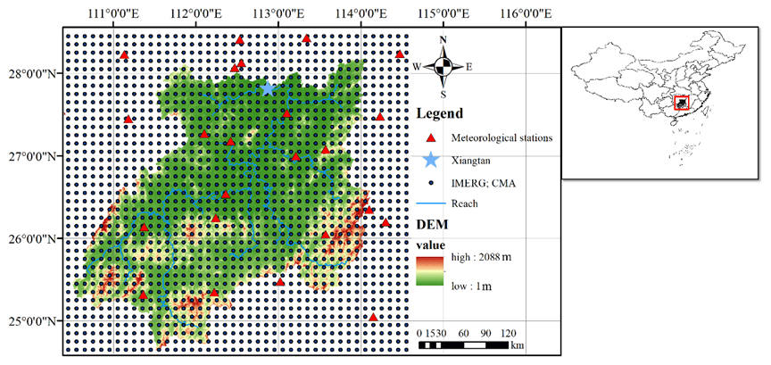
Figure 1 The spatial distribution of meteorological stations, the outlet of the study area and precipitation from IMERG and the CMA. Publisher's remark: please note that the above figure contains disputed territories.

Concentrated storm events during the flood season cause frequent floods throughout the basin. Since the Xiang River basin is the most densely populated and economically developed area in Hunan Province (Q. Zhu et al. 2020), it is critical to accurately simulate and predict flood events in the region for effective flood risk management.

2.2 Data description

IMERG V05B is a widely used satellite-based precipitation product with a spatiotemporal resolution of 0.1° and 30 min released by NASA, which consists of multiple rainfall retrieval algorithms and combines various precipitation-relevant remote sensing data sources obtained from the GPM sensors (Huffman et al., 2015). The IMERG system is firstly run twice to produce IMERG Early Run and IMERG Late Run (hereafter IMERG-E and IMERG-L) with latencies of 4 and 12 h in near real time (NRT). Then, through the bias adjustment with monthly Global Precipitation Climatology Centre (GPCC) gauge observations, IMERG Final Run (hereafter IMERG-F) is generated with 2.5 months of latency.

A precipitation product released by the China Meteorological Administration (hereafter the CMA), which merges rain gauge data from more than 30 000 automatic weather stations (AWSs) in China with the Climate Prediction Center MORPHing technique (CMORPH) precipitation product through an improved probability density function optimal interpolation method (PDF-OI), is used as the reference precipitation dataset in this study (Shen et al., 2014). The CMA provides precipitation estimates at a spatial resolution of 0.1° and a temporal resolution of 1 h, which is proven to be a reliable precipitation product as a result of the high density of the AWSs and the rigorous quality control of the source data. Therefore, the CMA has already been applied as a benchmark in some studies (Wang et al., 2017; Tang et al., 2017; Su et al., 2020).

Daily gauge meteorological variables (maximum and minimum temperature, relative humidity, wind speed and solar radiation) at 27 meteorological stations over the Xiang River basin are obtained from the CMA. The available hourly streamflow observation at the Xiangtan station is provided by the Hunan Hydrological Bureau of China. Figure 2 shows the time series of the hourly streamflow and the corresponding gauge-based precipitation between 2015 and 2017, where 11 historical flood events are selected with this study. The flood events are the streamflow time series with a 1-month span whose peak flow exceeded 8600 m³ s⁻¹, corresponding to approximately 97 times the quantile level (Q. Zhu et al., 2020). The period of the time series containing the selected flood events is from April 2014 to December 2017. The DEM (digital elevation model) with 90 m resolution is derived from NASA's Shuttle Radar Topographic Mission (SRTM) (Farr et al., 2007). Land cover and soil data with a resolution of 1 km are obtained from the Global Land Cover 2000 and Environmental and Ecological Science Data Center for West China as well as the National Natural Science Foundation of China, respectively.

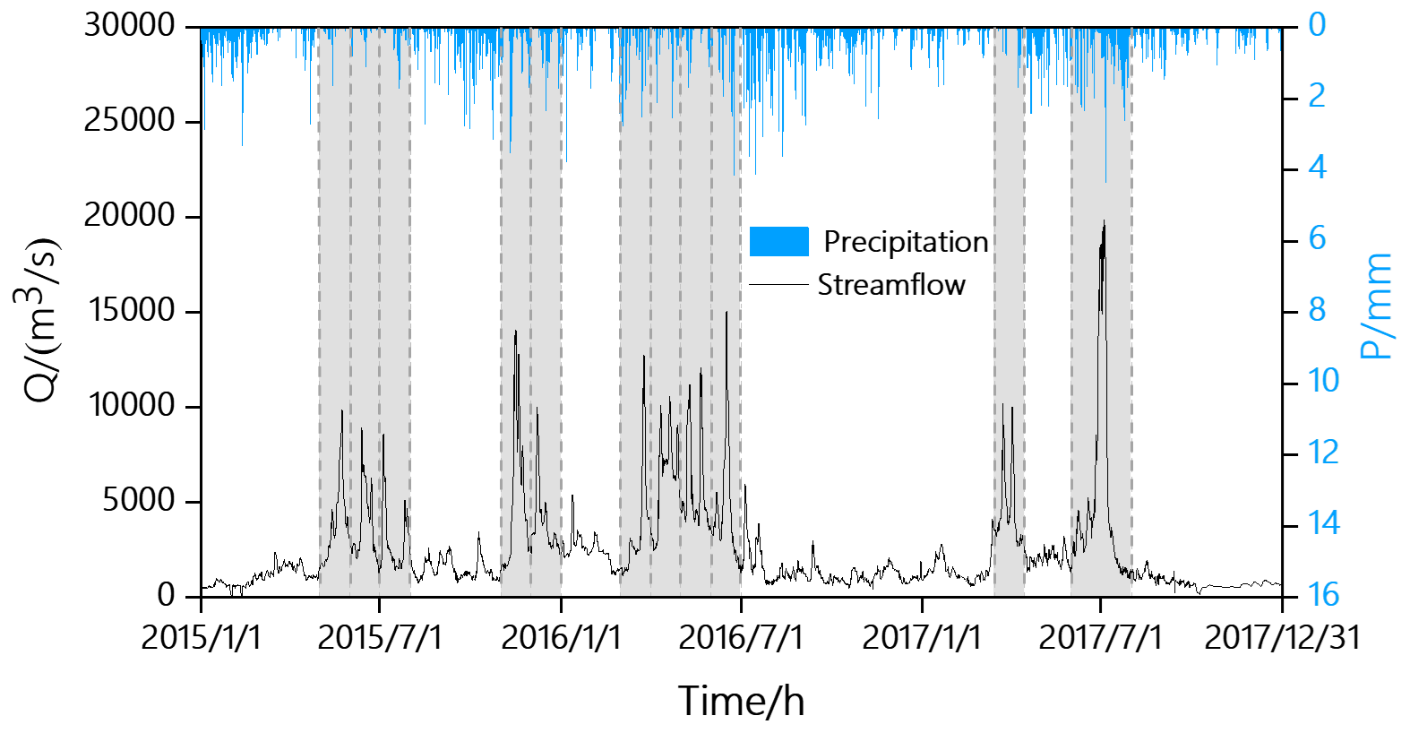
Figure 2 Time series of observed hourly streamflow at the Xiangtan station and basin-average precipitation from the CMA, with 11 selected flood events covered by shaded areas.

3 Methodology

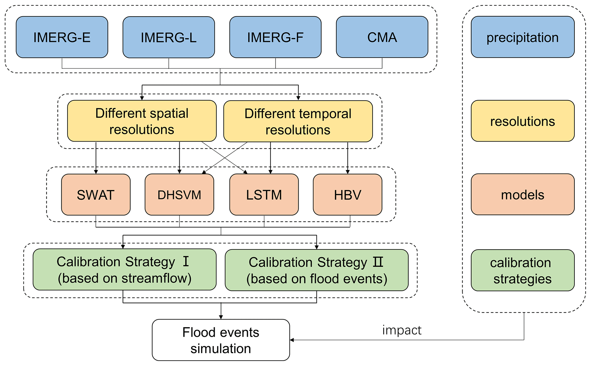
In this study, the IMERG precipitation products (IMERG-E, IMERG-L and IMERG-F) are assessed against the reference precipitation, i.e., the CMA, at different spatiotemporal resolutions. As mentioned above, three widely used and typical conceptual or physically based models (lumped HBV model, semi-distributed SWAT model and distributed DHSVM model) and one data-driven model (LSTM) are employed to probe the impacts of spatiotemporal resolutions of precipitation on flood event simulation. To investigate the impacts of spatial resolutions of precipitation on flood simulation, precipitation estimates with different spatial resolutions, which are obtained by inverse distance interpolation (Franke, 1982), are used to force the selected models, which are SWAT and DHSVM, as well as LSTM. To study the influence of temporal resolutions of precipitation on flood simulation, HBV, DHSVM and LSTM are utilized, which are forced by precipitation with different temporal resolutions. These four models are calibrated with two calibration strategies to investigate the potential benefits of the calibration strategy based on flood events. Finally, the performances of flood event simulation in different scenarios are compared and discussed. The designed framework for this study is shown in a flowchart in Fig. 3.

Figure 3 The methodological flowchart adopted in this study.

3.1 Hydrological models and LSTM

3.1.1 The HBV model

The conceptual HBV model was originally developed by the Swedish Meteorological and Hydrological Institute (SMHI) (Bergström and Forsman, 1973). Various versions of the HBV model have been developed and widely used in hydrological simulation and flood forecasting due to its simplicity and effectivity (Alfredsen and Hailegeorgis, 2015; Grimaldi et al., 2019; Huang et al., 2019). A lumped version of the HBV model (AghaKouchak et al., 2013) is used in this study, which is operated at hourly and daily time steps with the inputs of precipitation, temperature and potential evapotranspiration. The potential evapotranspiration is calculated with the Penman–Monteith equation (Beven, 1979) based on gauge meteorological data, and all the inputs are averaged over the basin with the Thiessen polygon method. Three main modules (soil moisture routine, response routine and transformation routine) are contained in the HBV model, while the module of the snow routine is not included in this case because of the temperature above 0^∘ C perennially over the Xiang River basin.

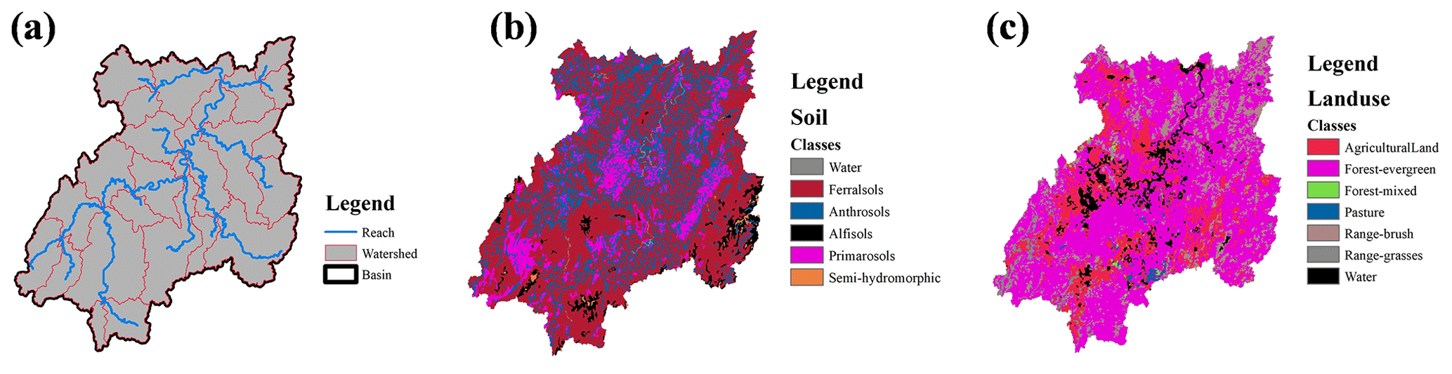
Figure 4 The (a) subbasin divisions, (b) soil types and (c) land use of the Xiang River basin used in the SWAT model.

3.1.2 The SWAT model

The SWAT model is a semi-distributed hydrological model developed by the Agricultural Research Center of the United States Department of Agriculture (USDA) (Arnold et al., 1998). SWAT 2012 is used in this study and is operated on a daily time step with the inputs of geographical data (DEM, land use and soil) (Fig. 4), precipitation and other meteorological variables mentioned above. The SWAT model divides the watershed into subbasins according to the DEM and then segregates them into multiple hydrological response units (HRUs) as the basic computational unit based on different types of soil, land use and slope. The Xiang River basin is divided into 25 subbasins and 495 HRUs in this study. Forest evergreen is the dominant land cover category with a coverage of 62 %, and Ferralsols is the main soil type with a coverage of 58 %, as shown in Fig. 4. The hydrologic cycle simulated by SWAT is based on the water balance equation, which mainly includes surface runoff, evapotranspiration, soil moisture and groundwater.

3.1.3 The DHSVM model

The DHSVM model is a fully distributed, physics-based hydrological model developed by the Pacific Northwest National Laboratory (PNNL) and the University of Washington (Wigmosta et al., 1994). DHSVM uses near-surface meteorology including air temperature, wind speed, humidity, precipitation, as well as incoming short- and long-wave radiation as hydroclimate inputs to solve energy and water balance. The model represents a dynamic watershed process at specific spatial scales considering the effect of topography, soil and vegetation. The DHSVM model mainly consists of seven modules, including an evapotranspiration module, a surface snowmelt module, a canopy snowmelt module, an unsaturated soil moisture module, a saturated soil flow module, a surface runoff module and a flow routing module. The version used in this study is DHSVM 3.1.2 with a grid resolution of 3000 m. Six soil types and eight vegetation classes are derived, and the spatial distributions of them are shown in Fig. 5.

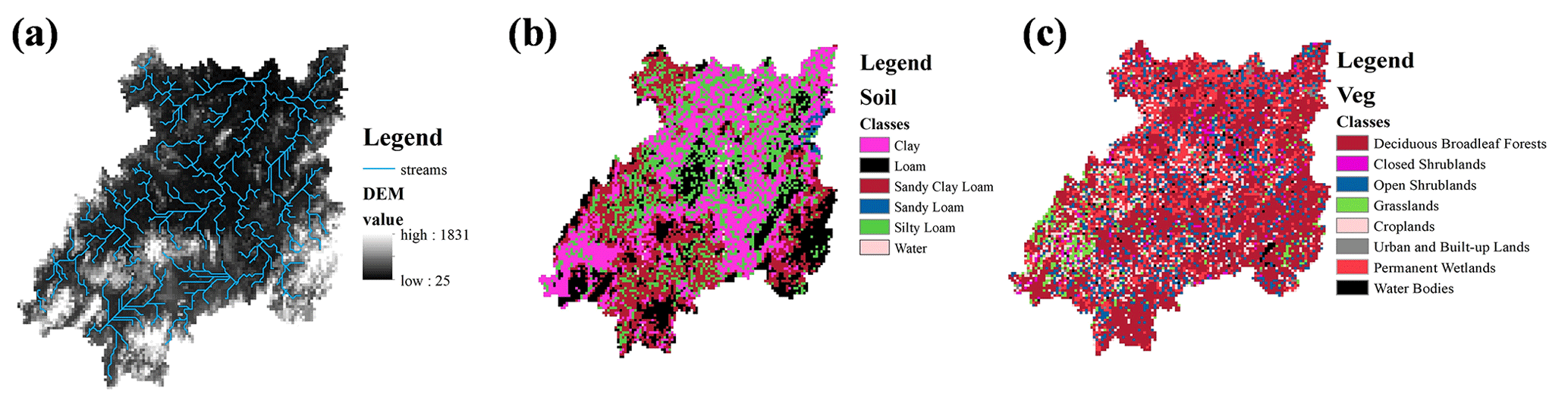
Figure 5 The (a) river network divisions, (b) soil types and (c) vegetation types of the Xiang River basin used in the DHSVM model.

3.1.4 The long short-term memory network

LSTM is a type of recurrent neural network (RNN) which was first proposed by Hochreiter and Schmidhuber (1997). LSTM is designed to overcome the error backflow problems with exploding and vanishing gradients by introducing three gates, i.e., forget, input and output gates, into the repeating modules of a neural network. The forget gate decides the information removed from the previous cell state. The input gate determines information updated to the present cell state, and the output gate controls which part of the cell state is output to the new hidden state. Therefore, LSTM can learn long-term dependencies between input and output features, which makes it appropriate for rainfall–runoff modeling. In this study, LSTM is developed using the deep learning framework PyTorch (Paszke et al., 2019), which has 100 hidden states and a single fully connected layer with a dropout rate of 0.5 (Srivastava et al., 2014). Precipitation and temperature are selected as the inputs of LSTM, and the output of LSTM is streamflow. The inputs for the complete sequence are x=[x₁, …, x_n], where x_t is a vector containing the input features of time t and the dimension of x_t corresponds to the number of grids of the precipitation data. The outputs for the complete sequence are y=[y₁, …, y_n], where y_t is the streamflow of time t.

3.2 Two strategies for parameter calibration

3.2.1 Calibration Strategy I

As stated above, almost all of the parameter calibration for hydrological modes is based on entire streamflow time series and is defined as Calibration Strategy I in this study. It is a conventional calibration method for optimizing the parameters of a hydrological model. For the HBV model, the whole period is divided into three periods: a warm-up period (April to December 2014), a calibration period (January 2015 to December 2016) and a validation period (January to December 2017). The calibration is conducted by maximizing the Nash–Sutcliffe efficiency coefficient (NSE) of the streamflow simulated during the calibration period via the SCE-UA algorithm (Duan et al., 1994).

For the SWAT model, the whole period is also divided into three periods, and they are the same as HBV. The calibration is accomplished with a separate tool named the SWAT Calibration and Uncertainty Program (SWAT-CUP) (Abbaspour et al., 2007). Parallel Sequential Uncertainty Fitting Version 2 (SUFI-2) is stable and always converging, and it is very appropriate for global optimization (Abbaspour et al. 2007), which is the reason why it is adopted in this study for parameter calibration. The objective function is also to reach the maximum value of NSE for the streamflow simulated in the calibration period.

The warm-up, calibration and validation periods of DHSVM are the same as HBV and SWAT as well as the objective function. The parameter calibration of DHSVM is executed by an autocalibration module based on ε-dominance non-dominated sorted genetic algorithm II (ε-NSGAII) (Pan et al., 2018). Parallel computing with a message-passing interface (MPI) program is applied in this study.

Regarding the training of LSTM, the learnable parameters of the network are updated depending on a given loss function. As with the selected hydrological models, the NSE is chosen as the objective criterion for LSTM (Kratzert et al., 2019), and adaptive moment estimation (Adam) (Kingma and Ba, 2014) with a learning rate of 0.0001 is used as the optimization algorithm. The dataset is generally divided into three parts, i.e., training, validation and test data. The first two parts are used to determine the parameters of the networks, and the last one is used to evaluate the performance of actual application. In this study, the whole dataset is divided into a training set (October 2015 to December 2017) and a validation set (April 2014 to September 2015). The absence of a test set is due to the limited available period of the data, while the selection of the training period will be discussed in detail in Sect. 5.3. Each LSTM network is trained with three different random initial seeds for 1500 epochs to account for the stochasticity in the network initialization. Of a total of 4500 trained models, the best model is selected through comprehensive consideration of both the calibration and validation NSE of the streamflow simulation.

3.2.2 Calibration Strategy II

Calibration Strategy II is designed in this study particularly for flood events and conducts the calibration based on the performance of flood event simulation. Eleven historical flood events that occurred between January 2015 and December 2017 are selected to conduct the flood event simulation (Fig. 2). The calibration is conducted by maximizing the mean NSE of the flood events simulated during the calibration period for the HBV model. For the SWAT and DHSVM models, numerous sets of parameters (the number is 1000 in this study) are obtained through the optimization algorithm, and the best-fitted parameter set is selected with the largest NSE for the flood event simulation. Considering LSTM, among a total of 4500 trained models, the best model is also selected by maximizing the mean NSE of the flood event simulation (four flood events during calibration and four flood events during validation).

3.3 Diagnostic statistics

To quantitatively evaluate the performance of streamflow and flood event simulation, three evaluation indices are selected in this study, i.e., NSE, BIAS-P and KGE. The formulas of these indices are listed as follows:

$$\begin{array}{}\text{(1)}& {\displaystyle }& {\displaystyle }\mathrm{NSE}=\mathrm{1}-{\displaystyle \frac{\sum _{t=\mathrm{1}}^T{\left(Q_{\mathrm{o}}^t-Q_{\mathrm{s}}^t\right)}^{\mathrm{2}}}{\sum _{t=\mathrm{1}}^T{\left(Q_{\mathrm{o}}^t-\stackrel{\mathrm{‾}}{Q_{\mathrm{o}}}\right)}^{\mathrm{2}}}},\text{(2)}& {\displaystyle }& {\displaystyle }\mathrm{BIAS}-P=\left|{\displaystyle \frac{Q_{\mathrm{s}}^{\mathrm{p}}-Q_{\mathrm{o}}^{\mathrm{p}}}{Q_{\mathrm{o}}^{\mathrm{p}}}}\times \mathrm{100}\right|,\text{(3)}& {\displaystyle }& {\displaystyle }\mathrm{KGE}=\mathrm{1}-\sqrt{(r-\mathrm{1}{)}^{\mathrm{2}}+(\mathit{\alpha }-\mathrm{1}{)}^{\mathrm{2}}+(\mathit{\beta }-\mathrm{1}{)}^{\mathrm{2}}},\end{array}$$

where $Q_{\mathrm{o}}^t$ and $Q_{\mathrm{s}}^t$ are the values of the observed and simulated flood events at time t, $Q_{\mathrm{o}}^{\mathrm{p}}$ and $Q_{\mathrm{s}}^{\mathrm{p}}$ are the observed and simulated flood peaks of the flood events, r is the linear correlation between observations and simulations, α is a measure of the flow variability error, and β is a bias term.

4 Results

4.1 The performance of flood event simulation based on two different calibration strategies

Figure 6 shows the distributions of NSE and BIAS-P values, which are used to evaluate the performance of four precipitation sources on flood events with two different calibration strategies at the daily scale.

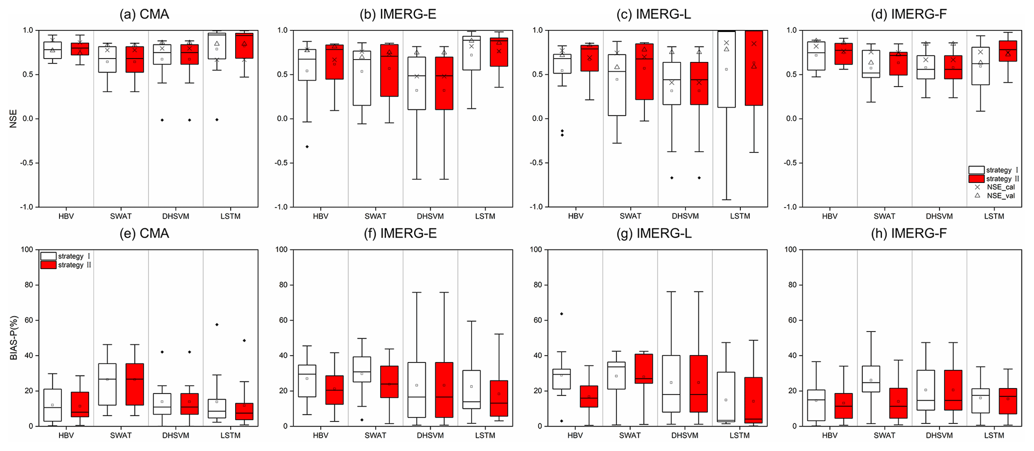
Figure 6 The NSE and BIAS-P of flood event simulation forced by (a, e) the CMA, (b, f) IMERG-E, (c, g) IMERG-L and (d, h) IMERG-F using two calibration strategies (the white box is based on Calibration Strategy I; the red box is based on Calibration Strategy II). The box plots show the 25th, 50th and 75th percentiles, and the mean value is given and shown with a square. The cross represents the NSE of simulated streamflow during calibration, and the triangle represents the NSE of simulated streamflow during validation.

For the performance of HBV, it can be seen that flood event simulation with Calibration Strategy II shows better performance. For the mean NSE, the values of the CMA, IMERG-E, IMERG-L and IMERG-F increase from 0.78, 0.54, 0.54 and 0.72 with Calibration Strategy I to 0.79, 0.62, 0.67 and 0.75, respectively, with Calibration Strategy II (Fig. 6). The corresponding mean BIAS-P values decrease from 12.0 %, 27.0 %, 29.0 % and 14.6 % to 11.4 %, 21.2 %, 16.7 % and 13.1 %. Meanwhile, the uncertainty of NSE and BIAS-P values of flood event simulation is reduced, with fewer occurrences of poor flood event simulation. The flood events simulated by the CMA have the highest NSE among all the precipitation sources, ranging from 0.61 to 0.95, and their averaged value is 0.79. This proves the capability of HBV in flood event simulation. When comparing the performance of IMERG precipitation estimates, IMERG-F performs best with both calibration strategies.

In terms of the streamflow and flood event simulation based on SWAT, Fig. 6 shows that the performance of the two calibration strategies with the CMA is comparable, while for IMERG precipitation estimates, Calibration Strategy II outperforms the other one. Specifically, for streamflow simulation, the NSE values in the validation period of IMERG-E, IMERG-L and IMERG-F show a significant increase from 0.70, 0.58 and 0.63 with Calibration Strategy I to 0.75, 0.78 and 0.73 with Calibration Strategy II, respectively. For flood event simulation, the mean NSE values based on Calibration Strategy II are 0.57, 0.58 and 0.63 forced with IMERG-E, IMERG-L and IMERG-F, which are 0.53, 0.44 and 0.57 based on Calibration Strategy I. The corresponding mean BIAS-P values are reduced from 29.8 %, 28.4 % and 26.1 % to 23.9 %, 28.0 % and 13.2 %. Compared to HBV and SWAT, the two calibration strategies present little difference in streamflow and flood event simulation based on DHSVM, which indicates that the performance of DHSVM is stable when using different calibration strategies.

For LSTM, the NSE values of flood event simulation also show higher mean values and smaller uncertainty based on Calibration Strategy II for all the precipitation products. The flood event simulation based on IMERG-L shows the most significant improvement, with the mean NSE value increasing from 0.62 with Calibration Strategy I to 0.77 with Calibration Strategy II. The flood event simulation based on the CMA and IMERG-E shows slightly lower medium NSE values of 0.94 and 0.88 with Calibration Strategy II than 0.95 and 0.99 with Calibration Strategy I. However, they show a higher 25th NSE with Calibration Strategy II, especially LSTM driven by IMERG-E, which increases from 0.58 with Calibration Strategy I to 0.66 with Calibration Strategy II. Therefore, although Calibration Strategy II has a lower median performance than Calibration Strategy I in individual cases, it still significantly improves the performance of LSTM, particularly in terms of uncertainty.

According to the above results, it can be concluded that Calibration Strategy II outperforms Calibration Strategy I. Therefore, the following parts are based on Calibration Strategy II.

4.2 Impact of the spatial resolutions of precipitation on flood event simulation

To investigate the impact of spatial resolutions of precipitation on flood event simulation, IMERG-E, IMERG-L, IMERG-F and the CMA are adopted to force the SWAT model, the DHSVM model and the LSTM model at 0.1, 0.25 and 0.5°, respectively.

Figure 7 shows the distributions of statistical indices, i.e., NSE, BIAS-P and KGE, which are used to evaluate the performance of different precipitation sources with different spatial resolutions in flood event simulation. From the BIAS-P of flood events simulated with SWAT, it can be seen that spatial resolution significantly affects the performance of precipitation in flood event simulation. For instance, the CMA performs best at 0.25° with the mean BIAS-P of 26.5 %, while IMERG-E, IMERG-L and IMERG-F display the best performance at 0.5° with mean BIAS-P values of 23.7 %, 22.9 % and 13.8 %, respectively. Similar to its performance in BIAS-P, in terms of the mean NSE, the CMA also performs best at 0.25° with a mean NSE of 0.66. IMERG-E presents little difference at different spatial resolutions, while IMERG-L performs slightly better at 0.5° with a mean NSE of 0.61 and a medium NSE of 0.76. The performance of IMERG-F gets worse as the resolution is coarser, regardless of the NSE or BIAS-P values. According to the KGE values, the performances based on the CMA, IMERG-E and IMERG-L show improvement at coarser spatial resolutions, except for IMERG-F, whose KGE values are stable at 0.71.

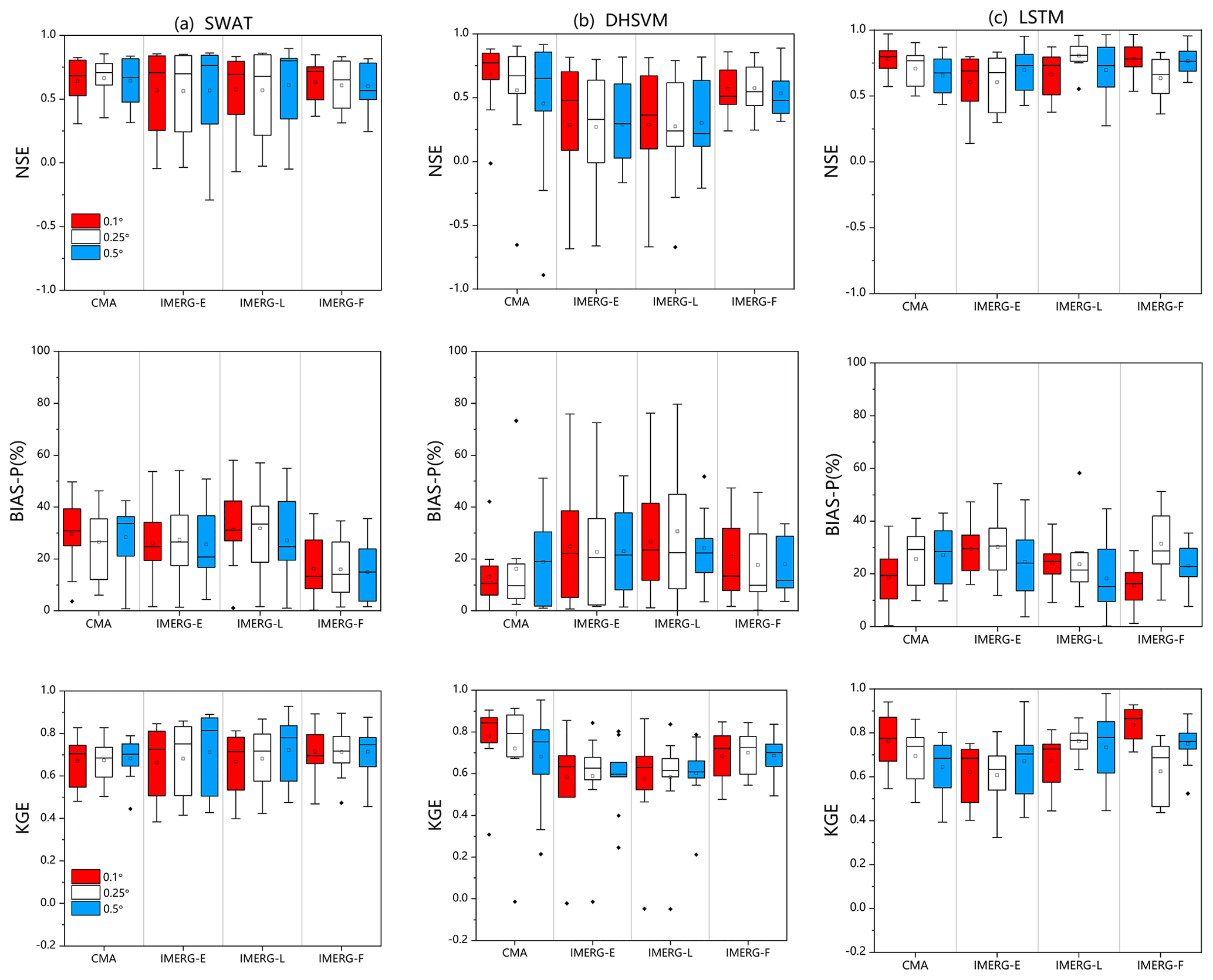
Figure 7 The performance of flood event simulation based on (a) SWAT, (b) DHSVM and (c) LSTM forced by precipitation with different spatial resolutions. The box plots show the 25th, 50th and 75th percentiles, and the mean value is given and shown with a square.

Compared to SWAT, DHSVM shows a different performance forced by precipitation with different spatial resolutions. The mean NSE of flood events simulated with the CMA declines from 0.68 to 0.45 when the spatial resolution of precipitation changes from 0.1 to 0.5°, the mean KGE declines from 0.77 to 0.66, and the mean BIAS-P increases from 13.9 % to 19.3 %. By contrast, the difference in flood events simulated with IMERG forcing at different spatial resolutions is smaller. For instance, the mean NSE values decrease from 0.29 to 0.27 for IMERG-E, from 0.30 to 0.29 for IMERG-L and from 0.58 to 0.53 for IMERG-F. However, the uncertainty of NSE, KGE and BIAS-P values of flood events simulated with IMERG decreases as the spatial resolution is finer. Of 11 flood event simulations, the performances of four flood event simulations get better as the spatial resolution gets coarser. The difference between the three IMERG precipitation estimates is illustrated clearly in Fig. 7b: the distributions of NSE, KGE and BIAS-P of simulated flood events forced with IMERG-E are more scattered than the others, while the uncertainty of IMGER-F is the smallest.

Similar to DHSVM, LSTM shows a different performance forced by precipitation with different spatial resolutions. The CMA and IMERG-F perform best at 0.1°, with mean BIAS-P values of 18.64 % and 15.55 % and mean NSE values of 0.78 and 0.78. The 25th NSE of flood events simulated with the CMA increases from 0.52 to 0.72, the 75th NSE increases from 0.78 to 0.83, and the spatial resolution is finer. The KGE shows the same pattern as NSE for the CMA and IMERG-F. By contrast, IMERG-E performs best at 0.5°, with a mean NSE of 0.69 and a medium NSE of 0.68, while IMERG-L performs best at 0.25°, with a mean NSE of 0.80 and a medium NSE of 0.81. In the light of BIAS-P, IMERG-E and IMERG-L achieve the best performance in flood event simulation at 0.5°, the mean values of which are 24.55 %, 18.27 % and 0.77 %. In contrast to BIAS-P, LSTM driven by IMERG-L shows the best KGE at 0.25° with a mean KGE of 0.76 and the smallest uncertainty, which is the same as NSE.

Compared with SWAT and DHSVM, LSTM shows better performance in flood event simulation. The mean NSEs of LSTM are higher than 0.7 in most cases, while the mean NSE of SWAT is around 0.6 and the largest mean NSE of DHSVM is 0.68. The 25th NSE of LSTM is higher than 0.5 in most cases, while the 25th NSE of DHSVM is around 0.15. The smallest 75th NSE of LSTM is 0.78, while the 75th NSE of DHSVM is around 0.6. The mean KGEs of SWAT and LSTM are similarly around 0.7 and are around 0.6 for DHSVM. In addition, LSTM also shows a relatively lower BIAS-P (mean values less than 25 %).

4.3 Impact of the temporal resolutions of precipitation on flood event simulation

To investigate the impact of temporal resolutions on flood event simulation, HBV, DHSVM and LSTM are adopted for forcing by the selected four precipitation sources at hourly and daily timescales. To compare the influences of temporal resolutions, the flood events simulated at the hourly scale are aggregated into daily time series.

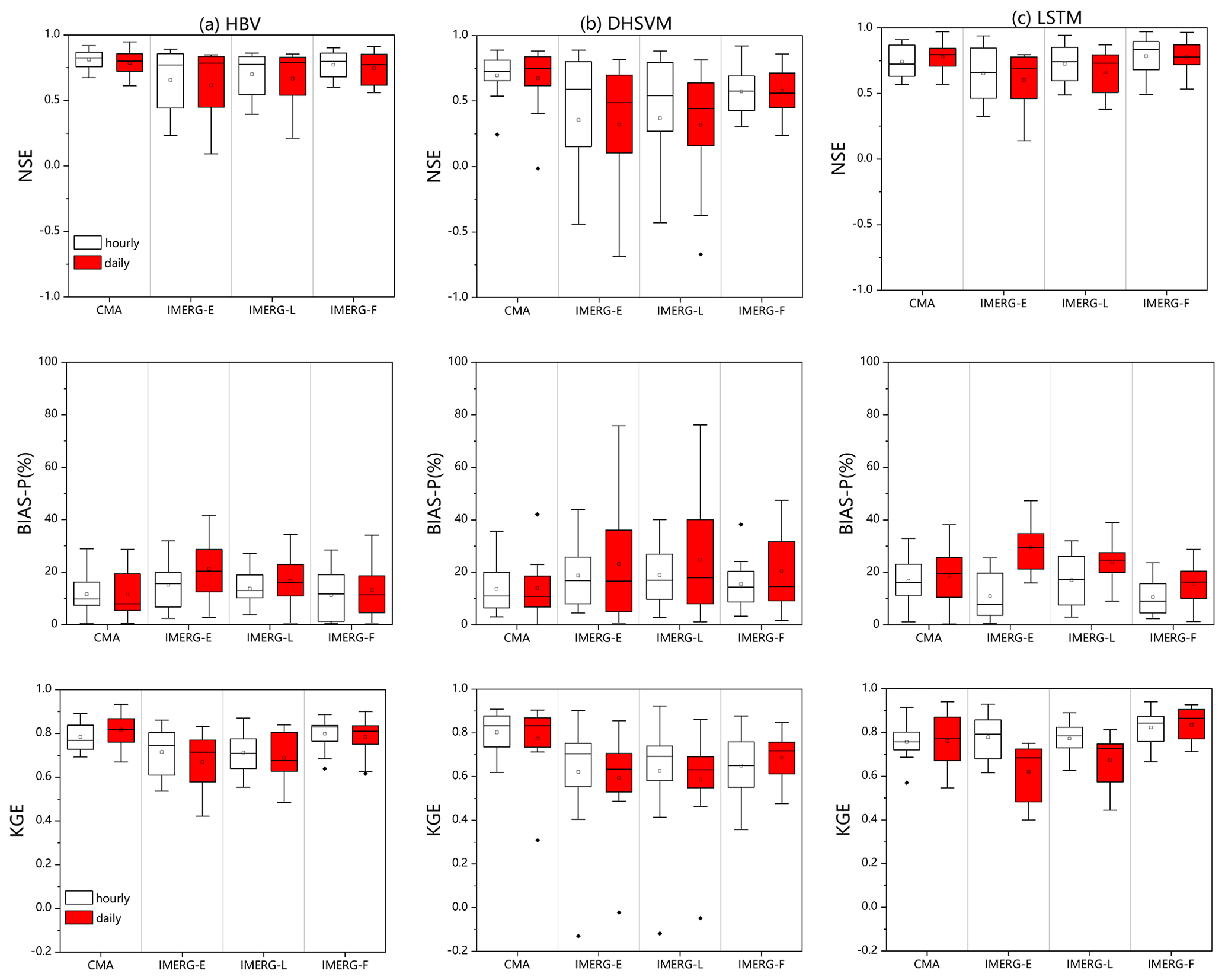
Figure 8 The performance of flood event simulation based on (a) HBV, (b) DHSVM and (c) LSTM forced by precipitation with temporal resolution. The box plots show the 25th, 50th and 75th percentiles, and the mean value is given and shown with a square.

The performance of different precipitation datasets with different temporal resolutions in flood event simulation is shown in Fig. 8. In HBV-based simulation, the mean NSE of the flood event simulation at the hourly scale is about 0.03 higher than that at the daily scale for all the precipitation products. The mean KGE of the flood event simulation at the hourly scale is also higher than that at the daily scale for IMERG forcing, while the mean KGE of flood events simulated with the CMA shows a decrease of about 0.03 at the hourly scale. In terms of BIAS-P, compared with the small difference between the performance of flood events simulated with the CMA at the hourly and daily scales, the performance of IMERG-E, IMERG-L and IMERG-F in flood event simulation at the hourly scale is much better than that at the daily scale (mean BIAS-P values of 15.1 % vs. 21.2 %, 13.7 % vs. 16.7 % and 11.1 % vs. 13.1 % for IMERG-E, IMERG-L and IMERG-F, respectively).

Similar performance is also presented in DHSVM-based simulation. According to the NSE and KGE values, the performances based on all the precipitation products show improvement at the hourly scale. More obvious improvement is shown in terms of BIAS-P, which decreases by 5 % at the hourly scale for IMERG products.

The performance based on LSTM is also shown in Fig. 8. Consistent with the results obtained by HBV and DHSVM, all the precipitation sources also have a relatively better performance at the hourly scale. For example, the mean BIAS-P of the CMA is reduced from 18.64 % at the daily scale to 16.7 % at the hourly scale. IMERG-E, IMERG-L and IMERG-F obtain better performance at the hourly scale with a mean NSE of 0.65, 0.73 and 0.78 and a mean KGE of 0.78, 0.77 and 0.82, respectively.

Compared with HBV and DHSVM, LSTM shows higher mean NSE values of flood event simulation, except for the simulation based on IMERG-L, while the HBV forced by the CMA and IMERG-F presents smaller uncertainty. In terms of BIAS-P, the two models show comparable performance, with mean values of around 15 %. The performance in the flood event simulation of HBV is more stable but slightly poorer than LSTM in general.

5 Discussion

5.1 Comparison of two different calibration strategies

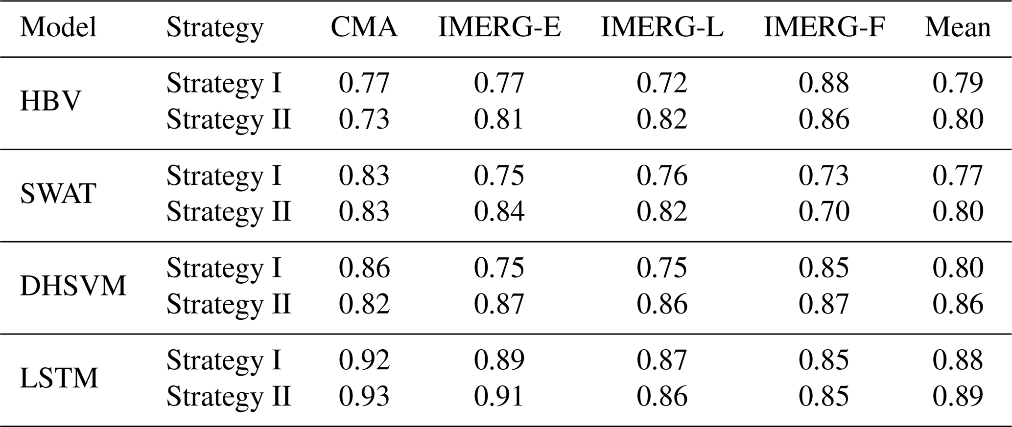
Two different calibration strategies are used to simulate flood events in this study. Compared with the conventional method for choosing the fit parameter set based on the entire streamflow time series (Calibration Strategy I), selecting the parameter set that results in the best flood event simulation (Calibration Strategy II) shows better performance in flood event simulation (Fig. 6). However, the CMA shows similar results under two different calibration strategies in SWAT-based flood event simulation, as does the DHSVM-based simulation. Furthermore, the CMA shows little difference with other precipitation forcing. Although we targeted differences between the two strategies in flood event simulation, their performances in the whole streamflow simulation time series are also compared, which is presented in Table 1 (the mean value is the average NSE of the four precipitation products with the same calibration strategy). According to the mean NSE values, Calibration Strategy II outperforms Calibration Strategy I. To be specific, for the HBV, SWAT, DHSVM and LSTM models, among the four precipitation products, there are two, three, three and three NSE values larger with Calibration Strategy II than with Calibration Strategy I. These findings indicate that both the precipitation accuracy and calibration strategy used in hydrological models are important uncertainty sources for flood simulation. From the lumped model to the distributed model, precipitation accuracy becomes the major source of uncertainty in streamflow or flood event simulation instead of the hydrological model, the reason for which is that hydrological models describe the hydrological process more and more comprehensively. In the application of LSTM for flood event simulation, a large number of equivalent simulations with different parameter sets is generated, which is similar to the parameter equifinality in hydrological simulation. When comparing the two calibration strategies, Calibration Strategy II is an effective way of training the LSTM model to obtain the best flood event simulation.

Table 1 The NSE values of the whole streamflow simulation time series forced by the CMA, IMERG-E, IMERG-L and IMERG-F.

5.2 Comparison of the performance of precipitation products in flood event simulation at different spatiotemporal resolutions

As illustrated in Figs. 7 and 8, the performance of precipitation products in flood event simulation is affected by both the spatial and temporal resolutions. Impacts of spatial resolution on flood event simulation behave differently among different models and precipitation sources. For the study area, at 0.25° spatial resolution, the CMA obtains the best flood event simulation based on SWAT. The impact of spatial resolution on the capture of precipitation variability during flood event periods can propagate to the flood event simulation. The best results are obtained at 0.25° spatial resolution: a possible reason can be that finer spatial resolution (0.1°) increases the uncertainty of precipitation sets. Nevertheless, coarser spatial resolution (0.5°) decreases the sufficiency of the datasets. For SWAT driven by the CMA, it shows the best 75th NSE and the worst 25th NSE at 0.5°, while the DHSVM driven by the CMA shows the same pattern at 0.5°, which proves that a coarser spatial resolution decreases the sufficiency of the datasets. However, the DHSVM driven by the CMA shows the best performance at 0.1°, which proves that the effects of increasing and decreasing spatial resolution are simultaneous and affect different models differently. This indicates that the choice of dataset is influenced by the resolution range, which must be adapted to the model definition, for the proper spatial resolution is essential to both minimizing the uncertainty and ensuring the sufficiency (Grusson et al., 2017).

The SWAT and DHSVM models driven by IMERG perform similarly at different spatial resolutions, which is consistent with previous research (Lobligeois et al., 2014; Huang et al., 2019), where an insignificant improvement was reported with a higher spatial resolution of observed rainfall in a large catchment area. This is probably due to the large catchment area, and only the outlet station is used for calibration. Liang et al. (2004) found a critical resolution ($\mathrm{1}/\mathrm{8}$° for the VIC model) for a watershed with 1233 km², beyond which the spatial resolution shows a limited impact on model performance. For our study area (82 375 km²), when the spatial resolution of precipitation changes from 0.1 to 0.5°, a small variation is shown in the performance of flood event simulation, which indicates that the critical resolution may be larger for a large watershed. For the data-driven model, the CMA and IMERG-F show better performance at 0.1° spatial resolution in the LSTM-based simulation, which indicates that a higher spatial resolution, i.e., a larger dataset, can improve the performance of flood event simulation. A similar conclusion is drawn from a previous study conducted by Sun et al. (2017), which also found that a deep learning model performs better with larger datasets. In addition, the simulation with IMERG-L and IMERG-E at 0.1° spatial resolution is not satisfactory, which may be related to the choice of hyperparameters and the limited data. However, after upscaling, the performance of LSTM in flood event simulation is greatly improved when the IMERG-L data are applied with 0.25° spatial resolution, which implies that scale transformation can be regarded as an approach of data enhancement in hydrological simulation based on deep learning.

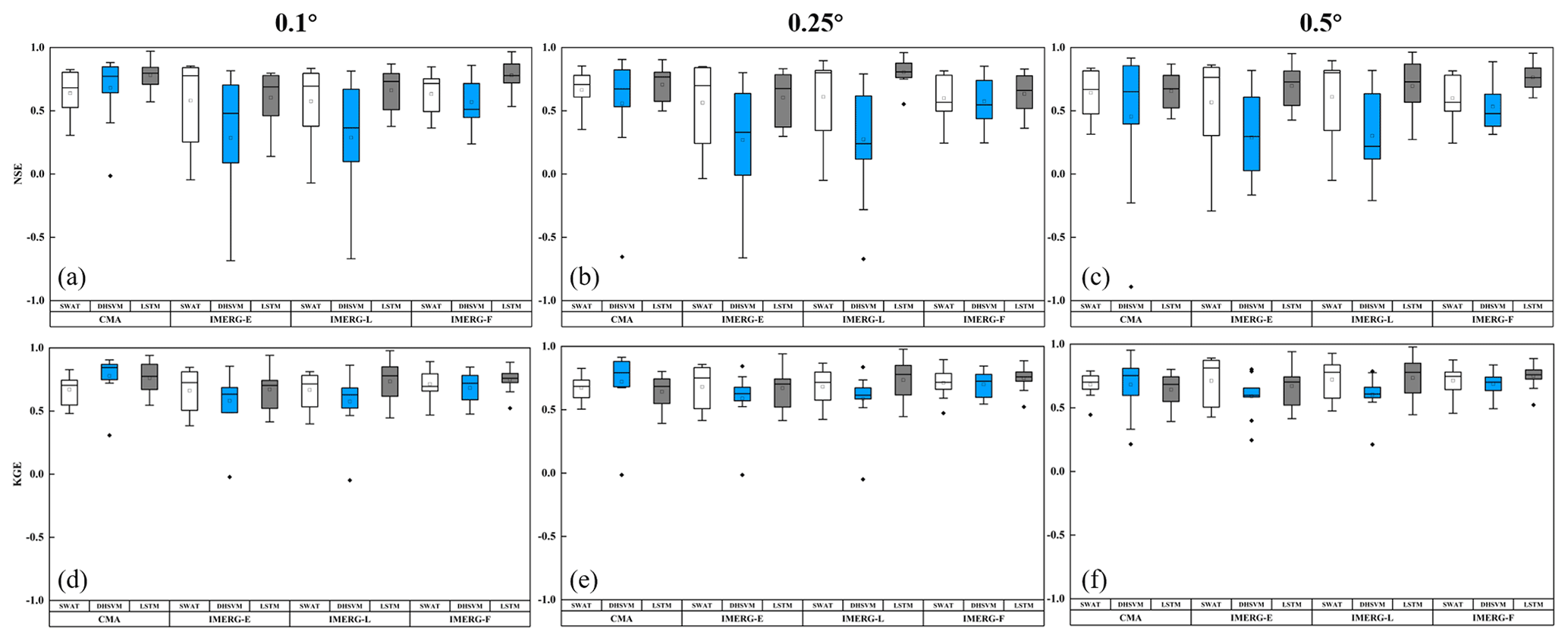
Figure 9 The NSE and KGE of flood event simulation forced by the CMA, IMERG-E, IMERG-L and IMERG-F with different spatial resolutions. The box plots show the 25th, 50th and 75th percentiles, and the mean value is given and shown with a square.

In order to compare the performance of different models on flood event simulation at the same spatial resolutions, some results presented in Fig. 7 are illustrated in Fig. 9. Overall, LSTM shows better performance in most cases. For instance, in Fig. 9a and c, LSTM is better than the other models, with the largest mean NSE and the smallest range between the 25th and 75th percentiles. There is also an exception. For example, in Fig. 9b, the range of NSE between the 25th and 75th percentiles of SWAT with the CMA is smaller than that of LSTM, but its mean and medium values of NSE are lower. Therefore, it can be summarized that the performance of LSTM has a higher likelihood of success than the other models. For KGE at 0.1° (Fig. 9d), LSTM also shows better performance than the other models, except for that simulated with the CMA, with which DHSVM is better than LSTM, and they show similar results with 0.5° (Fig. 9e).

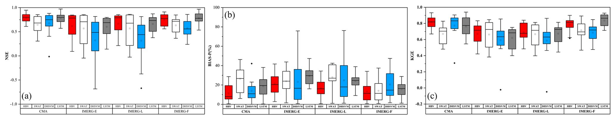
Figure 10 The (a) NSE, (b) BIAS-P and (c) KGE of flood event simulation forced by the CMA, IMERG-E, IMERG-L and IMERG-F using Calibration Strategy II. The box plots show the 25th, 50th and 75th percentiles, and the mean value is given and shown with a square.

The influence of spatiotemporal resolution on flood event simulation is affected by model structure. For instance, based on NSE, SWAT shows the best performance at 0.25° with CMA forcing, but LSTM shows the best performance at 0.1°. Similarly, based on KGE, SWAT performs the best at 0.5° with CMA forcing, but LSTM has the best performance at 0.1°. On the one hand, the difference in performance between NSE and KGE is due to their different statistical focus, with NSE giving larger weights to high values, especially flood peaks, which leads to different performance with different statistical metrics. On the other hand, the difference between SWAT and LSTM is due to their model structure. SWAT operates as a physically driven model, where the impact of the spatial resolution of the precipitation dataset will propagate during the hydrological process, which means that finer spatial resolution does not necessarily lead to the improved performance as indicated by studies such as Huang et al. (2019). This is probably exemplified by SWAT performing better at 0.25° with CMA forcing based on NSE, while it performs better at 0.5° based on KGE. Regarding LSTM as a deep learning model, some studies have highlighted significant performance enhancements when applied to larger, reliable datasets (Sun et al., 2017). Consequently, when forced by the CMA and IMERG-F, LSTM shows the best performance across all the statistical metrics at 0.1° rather than at 0.25 or 0.5°. The deviations from this pattern observed in IMERG-E and IMERG-L are likely attributable to inherent errors within the precipitation product itself. We previously evaluated the applicability of the IMERG dataset in the Xiangjiang River basin and found that IMERG-E and IMERG-L have larger uncertainties and errors than IMERG-F (Q. Zhu et al., 2020). The CMA has been confirmed by several studies to be a more reliable precipitation product in the Xiangjiang River basin and is always used as a reference precipitation product (Wang et al., 2017; Tang et al., 2017; Su et al., 2020). This probably makes IMERG-E and IMERG-L not bring enough performance improvement to LSTM when the spatial resolution is finer.

Considering the impacts of temporal resolutions on flood event simulation, for HBV and DHSVM, the flood event simulation at the hourly scale outperforms that at the daily scale in general, which indicates that a higher temporal resolution can improve the performance of hydrological models. Meanwhile, hourly precipitation sources also show better performance of flood event simulation with LSTM, especially for the simulation of flood peaks.

5.3 Comparison of different models in flood event simulation

In this study, a lumped hydrological model (HBV), a semi-distributed hydrological model (SWAT), a fully distributed hydrological model (DHSVM) and a data-driven model (LSTM) are utilized to simulate flood events. In order to compare the performance of different models in flood event simulation more clearly, some results presented in Fig. 6 are illustrated in Fig. 10. As shown in Fig. 10, HBV and SWAT forced by the CMA show comparable runoff simulation performance, while HBV shows better performance than SWAT in flood event simulation. The inability of the SWAT model to capture the flood events was also proven in previous studies (Zhu et al., 2016; Yu et al., 2018). Furthermore, when driven by IMERG, HBV outperforms SWAT and DHSVM, especially IMERG-E and IMERG-L. This is because the hydrological model with a simpler structure can reduce the impact of errors in radar rainfall estimation, which is better constrained during its propagation in the hydrological process (Zhu et al., 2013).

The comparisons of SWAT, DHSVM and LSTM at different spatial resolutions are also illustrated. As a data-driven approach, LSTM shows better performance than SWAT and DHSVM in terms of flood event simulation and shows reduced uncertainty and a higher likelihood of success than HBV, which is considered an appropriate model in this case. Among IMERG products, IMERG-F outperforms IMERG-E and IMERG-L in flood event simulation based on a hydrological model, while IMERG-E and IMERG-L show a comparable and even better performance than IMERG-F based on LSTM. This phenomenon shows that LSTM can deal with the error in precipitation products during the learning process. In many previous studies, LSTM is forced by large datasets such as the CAMELS dataset. The lower bound of the data requirements used for calibration is considered the daily time series of 15 years (Kratzert et al., 2019). In this study, as mentioned above, the calibration (October 2015 to December 2017) and validation (April 2014 to September 2015) of LSTM are different from those of hydrological models. For hydrological models, the calibration period is from January 2015 to December 2016 and the calibration period is from January to December 2017. We tried to use the same calibration data in LSTM as the hydrological model, but the results from flood event simulation are not satisfactory when its NSE of the validation period is less than 0.5. The reason is that two major flood events are not included in the calibration period used in the hydrological model. As a result, LSTM failed to learn the input–output relationship during the periods of flood events. Containing the characteristics of inputs as much as possible is critical for the data-driven model, e.g., LSTM, to capture the accurate relationship between the inputs and the output. Therefore, we use the data in the latter part for calibration, through which the performance of LSTM is significantly improved. It should be notable that reliance on data may still be a potential barrier to LSTM in data-sparse areas. In addition to obtaining more data for the input, such as the remote sensing data, how to make good use of limited data should also be considered in future studies. What is more, based on the same computer specification (Intel i5-9300H CPU, 8 GB memory), the running times of one simulation based on HBV, SWAT, DHSVM and LSTM are 0.2 s, 1 min, 54 min and 1.2 s, respectively. Results obtained from this case show that LSTM can provide reasonable accuracy in flood event simulation, whilst it is also competitive in computational efficiency.

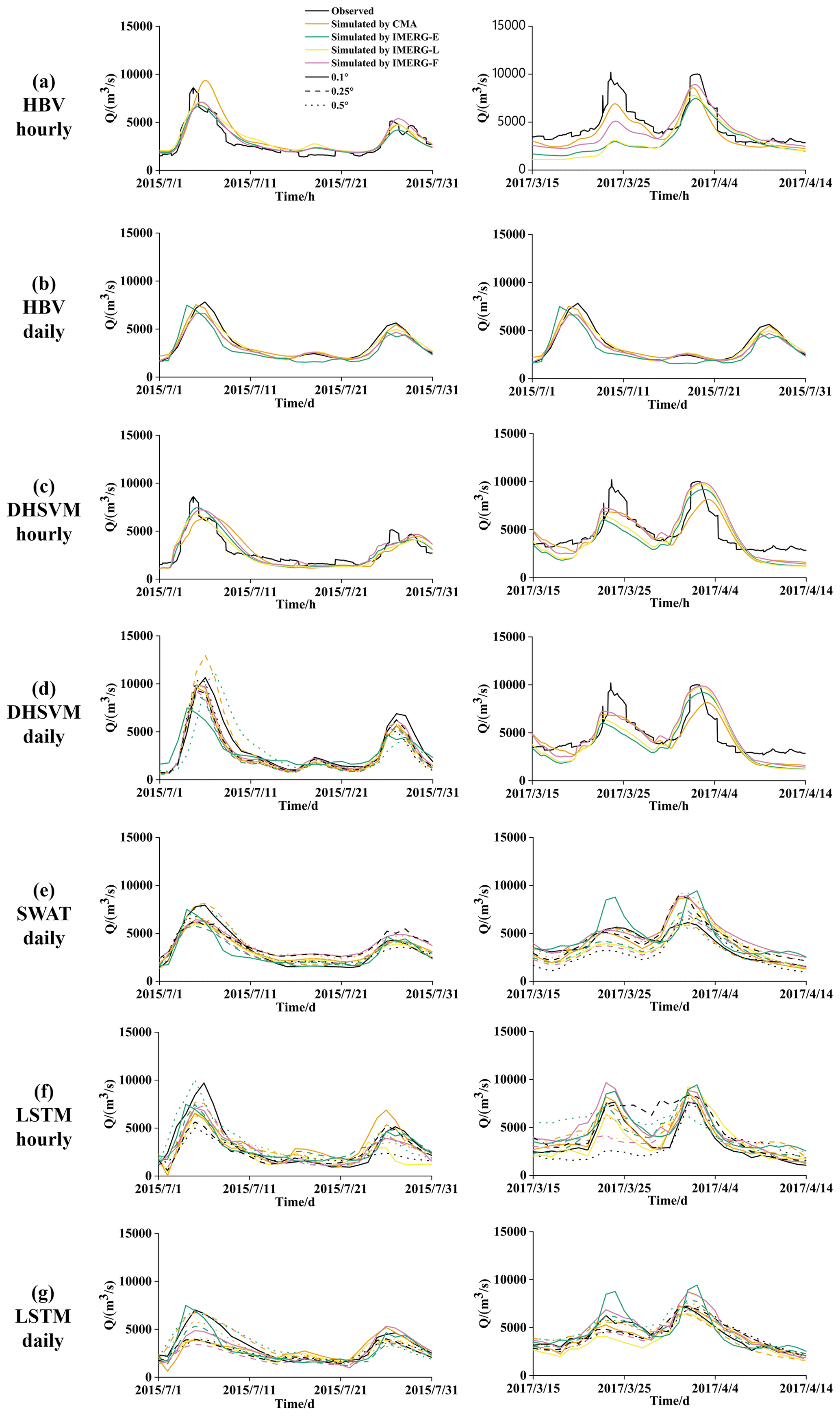
Figure 11 Comparison of HBV-, SWAT-, DHSVM- and LSTM-based flood event simulation from 1 to 31 July 2015 and from 15 March to 14 April 2017 forced by the CMA, IMERG-E, IMERG-L and IMERG-F with different spatiotemporal resolutions.

In order to compare the performance of flood event simulation with different scenarios, two randomly selected flood event simulations from 1 to 31 July 2015 and from 15 March to 14 April 2017 are shown in Fig. 11. The first flood event is the typical one with a single peak that occurred during the calibration period of the HBV, SWAT and DHSVM models and the latter one with twin peaks that occurred during the validation period of HBV, SWAT and DHSVM, while for LSTM the occurrence times of the two selected flood events are in its validation and calibration periods, respectively. From the figure, it can be seen that hydrological models generally show good ability to capture the first flood event. However, for the second flood event from 15 March to 14 April 2017, an obvious underestimation of the first peak exists in the flood simulation, which is primarily caused by the bias of precipitation products that are comprehensively evaluated in our previous study (Q. Zhu et al., 2020). The underestimation of the second flood peak is reduced in LSTM-based simulations, which implies the ability of LSTM to correct the propagation of influence from the bias of precipitation. Since the hydrological models may smoothen the short-term variability of input, the flood events simulated with hydrological models show relatively smooth runoff processes compared with LSTM. Meanwhile, the performance of LSTM is not stable at different spatial resolutions compared with SWAT and DHSVM. Compared with spatiotemporal resolutions of precipitation and simulation models, the precipitation source is the primary uncertainty source for flood event simulation, which indicates the importance of choosing an appropriate precipitation source for ungauged regions.

6 Conclusion

In this study, we investigated the impacts of temporal and spatial resolutions of precipitation on flood event simulation over a large-scale catchment. We accomplished the study with the application of HBV, SWAT, DHSVM and LSTM forced by high-spatiotemporal-resolution gauge-based and satellite-based precipitation products. The main conclusions of this study are summarized as follows.

1. According to the comparison of two calibration strategies, an event-based calibration strategy leads to better performance of flood event simulation based on a lumped HBV model and a semi-distributed SWAT model. However, there is little difference between the two calibration strategies' applications to a distributed DHSVM model. For the data-driven model, LSTM, the event-based strategy also leads to better results.

2. Considering the impact of temporal resolution, both hydrological models and LSTM perform better at the hourly scale in flood event simulation than at the daily scale, especially in flood peaks. However, the influence of spatial resolution on flood event simulation has no significant pattern in this case, which varies with models and precipitation sources.

3. Three hydrological models and LSTM are used to simulate the flood events forced by gauge-based and satellite-based precipitation products in this study. The hydrological models and LSTM forced by IMERG precipitation estimates can achieve acceptable flood event simulation in most cases. In some cases, LSTM outperforms the hydrological models. However, it should be noted that the performance of LSTM largely depends on the input data and settings, such as the choice of hyperparameters, which may be unstable in some other cases.

Appendix A

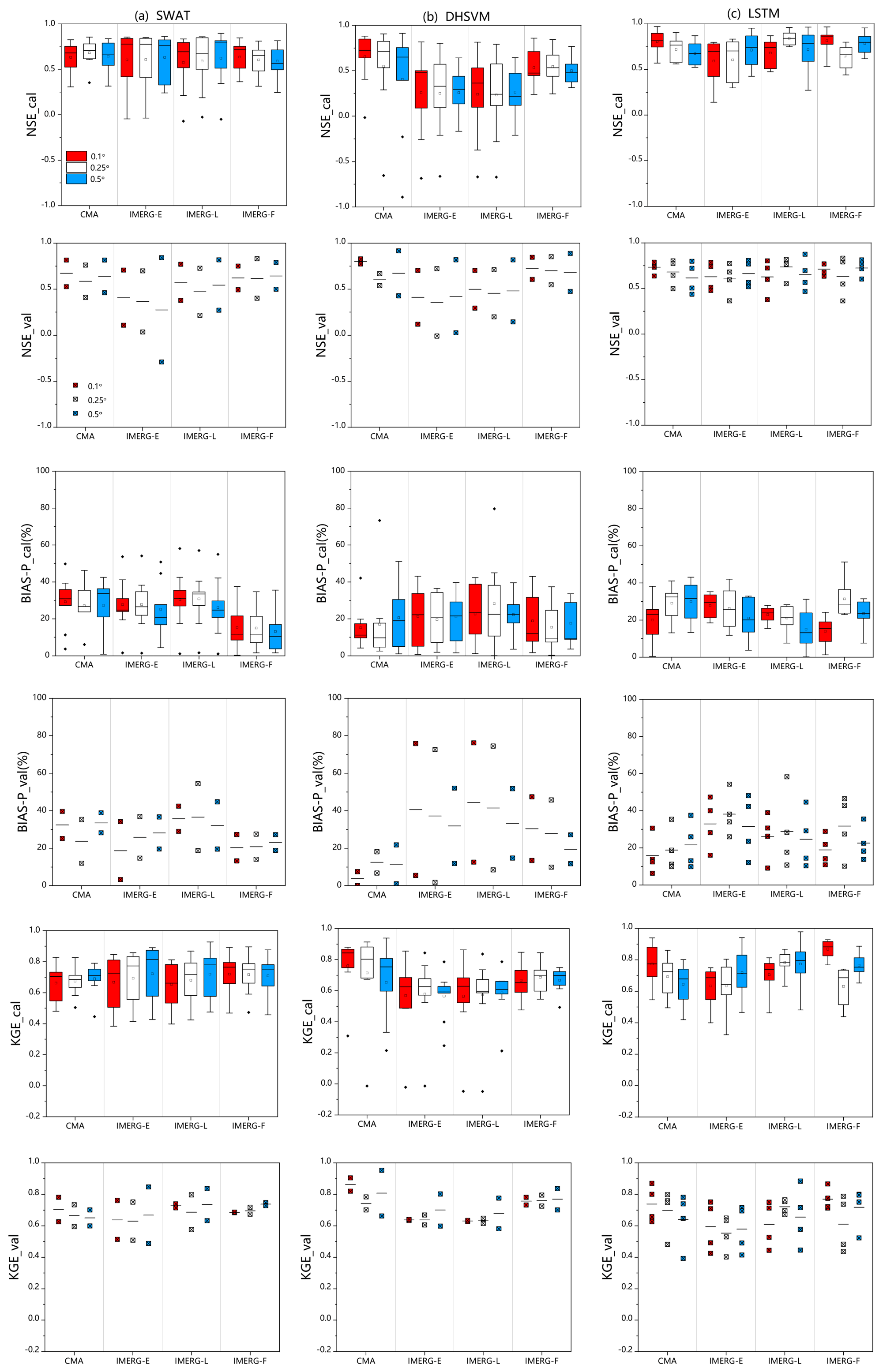
Figure A1 Same as Fig. 7, but the results in calibration and validation periods are separated.

Appendix B

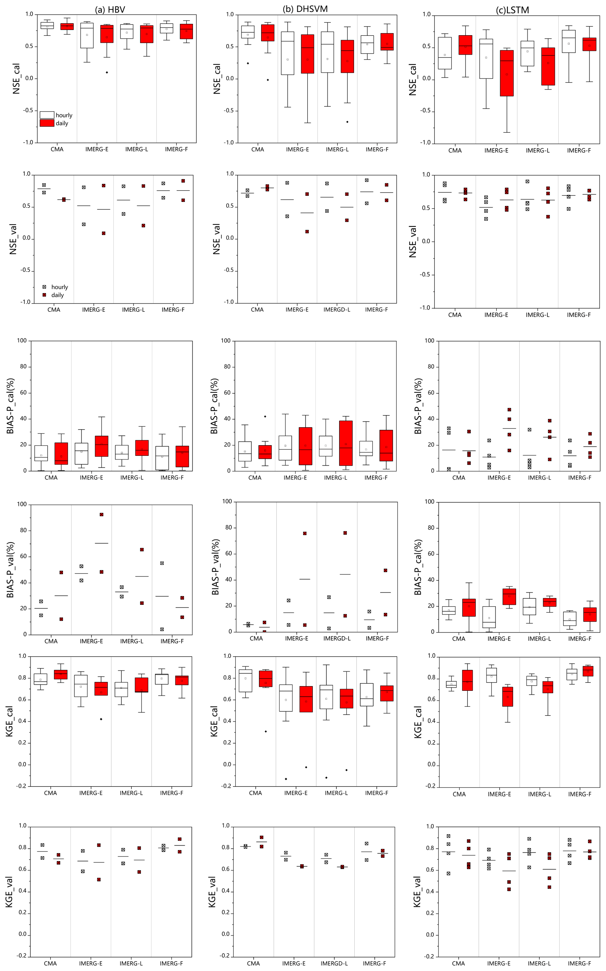
Figure B1 Same as Fig. 8, but the results in calibration and validation periods are separated.

Appendix C

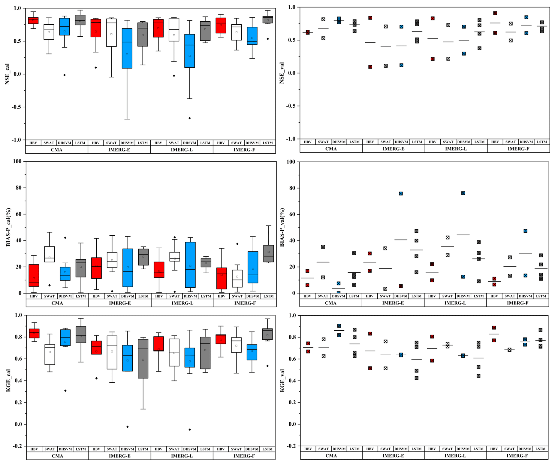
Figure C1 Same as Fig. 10, but the results in calibration and validation periods are separated.