Multi-model approach in a variable spatial framework for streamflow simulation

Accounting for the variability of hydrological processes and climate conditions between catchments and within catchments remains a challenge in rainfall–runoff modelling. Among the many approaches developed over the past decades, multi-model approaches provide a way to consider the uncertainty linked to the choice of model structure and its parameter estimates. Semi-distributed approaches make it possible to account explicitly for spatial variability while maintaining a limited level of complexity. However, these two approaches have rarely been used together. Such a combination would allow us to take advantage of both methods. The aim of this work is to answer the following question: what is the possible contribution of a multi-model approach within a variable spatial framework compared to lumped single models for streamflow simulation?

To this end, a set of 121 catchments with limited anthropogenic influence in France was assembled, with precipitation, potential evapotranspiration, and streamflow data at the hourly time step over the period 1998–2018. The semi-distribution set-up was kept simple by considering a single downstream catchment defined by an outlet and one or more upstream sub-catchments. The multi-model approach was implemented with 13 rainfall–runoff model structures, three objective functions, and two spatial frameworks, for a total of 78 distinct modelling options. A simple averaging method was used to combine the various simulated streamflow at the outlet of the catchments and sub-catchments. The lumped model with the highest efficiency score over the whole catchment set was taken as the benchmark for model evaluation.

Overall, the semi-distributed multi-model approach yields better performance than the different lumped models considered individually. The gain is mainly brought about by the multi-model set-up, with the spatial framework providing a benefit on a more occasional basis. These results, based on a large catchment set, evince the benefits of using a multi-model approach in a variable spatial framework to simulate streamflow.

1 Introduction

1.1 Uncertainty in rainfall–runoff modelling

A rainfall–runoff model is a numerical tool based on a simplified representation of a real-world system, namely the catchment (Moradkhani and Sorooshian, 2008). It usually computes streamflow time series from climatic data, such as rainfall and potential evapotranspiration. Many rainfall–runoff models have been developed according to various assumptions in order to meet specific needs (e.g. water resources management, flood and low-flow forecasting, hydroelectricity), with choices and constraints concerning the following (Perrin, 2000):

• the temporal resolution, i.e. the way variables and processes are aggregated over time;

• the spatial resolution, i.e. the way spatial variability is taken into account more or less explicitly in the model;

• the description of dominant processes.

Different models will necessarily produce different streamflow simulations. Intuitively, one often expects that working at a finer spatio-temporal scale should allow for a better description of the processes (Atkinson et al., 2002). However, this generally leads to additional complexity, i.e. a larger number of parameters, which requires more information to be estimated and often yields more uncertain results (Her and Chaubey, 2015).

Uncertainty in rainfall–runoff models depends on the assumptions made regarding the choice of the general structure and also on the parameter estimates. The variety of model structures and equations results in a large variability of streamflow simulations (Ajami et al., 2007). The spatial and temporal resolutions also result in different streamflow simulations. Due to the complexity of the real system and the lack of information to parameterize the various equations over the whole catchment, parameter estimates must be set. Usually, these parameters are determined for each entity of interest by minimizing the error induced by the simulation compared to an observation. The choice of the optimization algorithm, the objective function, and the streamflow transformation is therefore also a source of uncertainty. Since input data are used to derive model structures and parameters, the uncertainty associated with these data also contributes to the overall model uncertainty (Beven, 1993; Liu and Gupta, 2007; Pechlivanidis et al., 2011; McMillan et al., 2012).

Various approaches aim to improve models by taking uncertainties into account, among which are multi-model approaches, which are the main topic of our research.

1.2 Multi-model approach

The multi-model approach consists in using several models in order to take advantage of the strengths of each one. This concept has been gaining momentum in hydrology since the end of the 20th century for simulation (e.g. Shamseldin et al., 1997) and forecasting (e.g. Loumagne et al., 1995). In this section, we distinguish between probabilistic and deterministic approaches.

A probabilistic multi-model approach seeks an explicit quantification of the uncertainty associated with simulations or forecasts through statistical methods. The ensemble concept has commonly been applied in meteorology for several decades, and subsequently has been widely used in hydrology to improve prediction (i.e. simulation or forecast). The international Hydrologic Ensemble Prediction Experiment initiative (Schaake et al., 2007) fostered the work on this topic. The ensemble concept has also been adapted to rainfall–runoff models in order to reduce modelling bias: Duan et al. (2007) used multiple predictions made by several rainfall–runoff models using the same hydroclimatic forcing variables. An ensemble consisting of nine different models (from three different structures and parameterizations) was constructed and applied to three catchments in the United States. The predictions were then combined through a statistical procedure (Bayesian model averaging or BMA), which assigns larger weight to a probabilistic likelihood measure. The authors showed that the probabilistic multi-model approach improves flow prediction and quantifies model uncertainty compared to using a single rainfall–runoff model. Block et al. (2009) coupled both multiple climate and multiple rainfall–runoff models, increasing the pool of streamflow forecast ensemble members and accounting for cumulative sources of uncertainty. In their study, 10 scenarios were built for each of the three climatic models and applied to two rainfall–runoff models, i.e. 60 different forecasts. This super-ensemble was applied to the Iguatu catchment in Brazil and showed better performance than the hydroclimatic or rainfall–runoff model ensembles studied separately. Note that the authors tested three different combination methods: pooling, linear regression weighting, and a kernel density estimator. They found that the last technique seems to perform better. Velázquez et al. (2011) showed that the combination of different climatic scenarios with several models in a forecasting context leads to a reduction in uncertainty, particularly when the forecast horizon increases. However, such methods generate a large number of scenarios and can therefore become time-consuming and difficult to analyse. The probabilistic combination of simulations remains a major topic in the scientific community (see Bogner et al., 2017).

A deterministic multi-model approach seeks to define a single best streamflow time series, which often consists in a combination of the simulations of individual models. Shamseldin et al. (1997) tested three methods in order to combine model outputs: a simple average, a weighted average, and a non-linear neural network procedure. Their study was conducted on a sample of 11 catchments mainly located in southeast Asia using five different lumped models operating at the daily time step and showed that multiple models perform better than models applied individually. Similar conclusions were reached in the Distributed Model Intercomparison Project (DMIP) (Smith et al., 2004) conducted by Georgakakos et al. (2004) in simulation or by Ajami et al. (2006) for forecasting. In both articles, 6 to 10 rainfall–runoff models were applied at the hourly time step over a few catchments in the United States. These studies showed that a model that performs poorly individually can contribute positively to the multi-model set-up. Winter and Nychka (2010) specify that the composition of the multi-model set-up is important. Indeed, using 19 global climate models, the authors have shown that simple – or weighted – average combinations are more efficient if the individual models used produce very different results. Studies combining rainfall–runoff models by machine learning techniques led to the same conclusions (see, for example, Zounemat-Kermani et al., 2021, for a review).

All of the aforementioned multi-model approaches only focus on the structural aspect of rainfall–runoff models. Some authors have also combined streamflow generated from different parameterizations of the same rainfall–runoff model. Oudin et al. (2006) proposed combining two outputs obtained with a single model (GR4J) from two calibrations, one adapted to high flows and the other to low flows, by weighting each of the simulations on the basis of a seasonal index (filling rate of the production reservoir). Such a method makes it possible to provide good efficiency in both low and high flows, whereas usually an a priori modelling choice must be made to focus on a specific streamflow range. More recently, Wan et al. (2021) used a multi-model approach based on four rainfall–runoff models calibrated with four objective functions on a large set of 383 Chinese catchments. The authors showed that methods based on weighted averaging outperform the ensemble members, except in low-flow simulation. They also highlighted the benefit of using several structures with different objective functions. The size of the ensemble was also studied, and it was found that using more than nine ensemble members does not further improve performance. Note that different results for optimal size can be found in the literature (Arsenault et al., 2015; Kumar et al., 2015).

The aforementioned studies were carried out within a fixed spatial framework (e.g. lumped, semi-distributed, distributed), i.e. considering that the model structures implemented are relevant over the whole modelling domain. Implicitly, the underlying assumption is that a fixed rainfall–runoff model can capture the main hydrological processes affecting streamflow in a catchment (and its sub-catchments). However, this may not be true. Introducing a variable spatial modelling framework into the multi-model approach could help to overcome this issue.

1.3 Scope of the paper

This study intends to test whether streamflow simulation can be improved through a multi-model approach. More precisely, we aim here to deal with the uncertainty stemming from (i) the spatial dimension (e.g. catchment division, aggregation of hydroclimatic forcing, boundary conditions), (ii) the general structure of the model (e.g. formulation of water storages, filling/draining equations), and (iii) the parameter estimation (e.g. calibration algorithm, objective function, calibration period). However, we decided here not to focus on quantifying these uncertainties individually (as it could be done with a probabilistic ensemble), but we focus on the aggregated impact of all uncertainties through comparing the deterministic averaging combination of several models with a single one. Ultimately, our aim is to answer the following question: what is the possible contribution of a multi-model approach within a variable spatial framework compared to lumped single models for streamflow simulation?

This study follows on from the work of Squalli (2020), who carried out exploratory multi-model tests on lumped and semi-distributed configurations at a daily time step. The remainder of the paper is organized as follows: first, the catchment set, the hydroclimatic data, the spatial framework, and the rainfall–runoff models used for this work are presented. The multi-model methodology and the calibration/evaluation procedure are described. Then we present, analyse, and discuss the results. Last, we summarize the main conclusions of this work and discuss its perspectives.

2 Material and methods

2.1 Catchments and hydroclimatic data

This study was conducted at an hourly time step using precipitation, potential evapotranspiration and streamflow time series over the period 1998–2018 (Delaigue et al., 2020). Precipitation (P) was extracted from the radar-based COMEPHORE re-analysis produced by Météo-France (Tabary et al., 2012), which provides information at a 1 km² resolution and which has already been extensively used in hydrological studies (Artigue et al., 2012; van Esse et al., 2013; Bourgin et al., 2014; Lobligeois et al., 2014; Saadi et al., 2021).

Potential evapotranspiration (E₀) is calculated with the formula proposed by Oudin et al. (2005). This equation was chosen for its simplicity, as the only input required is daily air temperature (from the SAFRAN re-analysis of Météo-France; see Vidal et al., 2010) and extra-terrestrial radiation (which only depends on the Julian day and the latitude). Once calculated, the daily potential evapotranspiration was disaggregated to the hourly time step using a simple parabola (Lobligeois, 2014). These steps for converting daily temperature data into hourly potential evapotranspiration are directly possible in the airGR software (Coron et al., 2017, 2021; developed using the R programming language; R Core Team, 2020), which was used for this work. We did not use any gap-filling method since all climatic data were complete during the study period.

Streamflow time series (Q) were extracted from the national streamflow archive Hydroportail (Dufeu et al., 2022), which makes the data produced by hydrometric services in regional environmental agencies in charge of measuring flows in France, as well as by other data producers (e.g. hydropower companies and dam managers), available. Before being archived, flow data undergo quality control procedures applied by data producers, with corrections when necessary. Quality codes are also available, although this information is not uniformly provided for all stations. These data are freely available on the Hydroportail website and are widely used in France for hydraulic and hydrological studies.

Here, we focus on simulating streamflow at the main catchment outlet, addressing the issue from a large-sample-hydrology (LSH) perspective (Andréassian et al., 2006; Gupta et al., 2014), in which many catchments are used. For this study, 121 catchments spread over mainland France with limited human influence were selected (Fig. 1). The first criterion used to select catchments is based on streamflow availability. Here, a threshold of 10 % maximum gaps per year over the whole period was considered (1999–2018). However, this criterion may be slightly too restrictive (e.g. removal of a station installed in 2000 and presenting continuous data since then). In order to overcome this problem, we decided to allow this threshold to be exceeded for a maximum of 3 years over the whole period considered. It is therefore a compromise between having a large number of catchments for the study and having a long enough period for model calibration and evaluation. The catchment selection also considered the level of human influence. In France, the vast majority of catchments have human influence (e.g. dams, dikes, irrigation, or urbanization). Here, streamflow with limited human influence corresponds to gauged stations where the streamflow records have a hydrological behaviour considered close enough to a natural streamflow (e.g. low water withdrawals, influences far enough upstream to be sufficiently diluted downstream) not to strongly limit model performance. This was based on numerical indicators on the influence of dams and local expertise. Although snow-dominant or glacial regimes were rejected (due to lack of data or anthropogenic influence), the various catchments selected offer a wide hydroclimatic variability (Table 1).

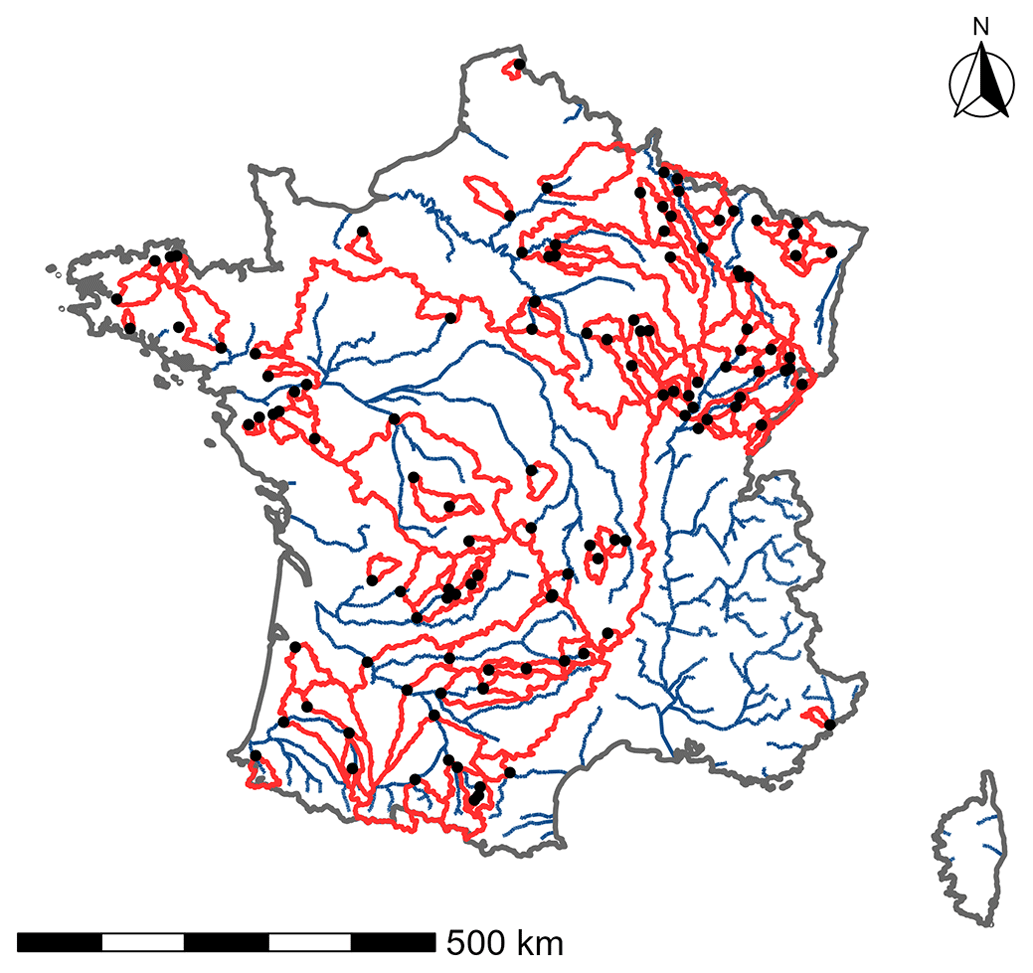
Figure 1 Boundaries (in red) and outlets (black dots) of the 121 catchments selected for this study.

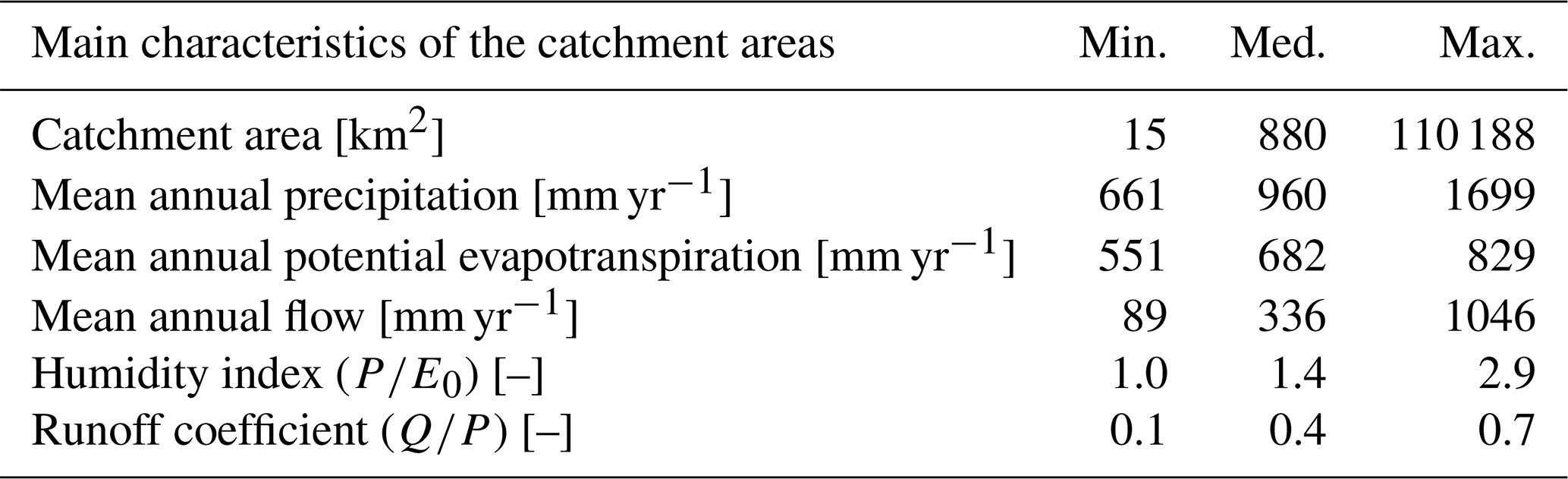
Table 1 Minimum, median, and maximum values of some characteristics of the 121 catchments (P stands for mean annual precipitation, E₀ for mean annual potential evapotranspiration, Q for mean annual flow).

2.2 Principle of catchment spatial discretization

In this work, two spatial frameworks are used: lumped and semi-distributed. A lumped model considers the catchment as a single entity, while the semi-distribution seeks to divide this catchment into several sub-catchments in order to partly take into account the spatial variability of hydroclimatic forcing and physical characteristics within the catchment.

Generally, the division of a catchment is defined on the basis of expertise and requires good knowledge of its characteristics (hydrological response units based on geology or land use). From a large-sample hydrology perspective, an automatic definition of semi-distribution was needed. To this end, we simplified the problem by looking at a first-order distribution, i.e. a single downstream catchment defined by an outlet and one or more upstream sub-catchments. The underlying assumption is therefore that a second-order distribution (i.e. further dividing the upstream sub-catchments into a few smaller sub-catchments) will have a more limited impact on model behaviour than the first, when considering the main downstream outlet. This assumption is based on the work of Lobligeois et al. (2014) which showed that a multitude of sub-basins of approximately 4 km² provide limited gain compared to a few sub-catchments of 64 km². Under these hypotheses, we developed an automatic procedure to select semi-distributed configurations nested in each other, which we termed “Matryoshka doll”. This approach consists in creating different simple and distinct combinations of upstream–downstream gauged catchments starting from the main downstream station and progressively moving upstream.

Specifically, the Matryoshka doll selection approach (Fig. 2) was implemented as follows:

1. Select a downstream station defining a catchment with one or more gauged internal points.

2. Restrict the upstream sub-catchment partitioning to a first-order split, i.e. going back only to the nearest upstream station(s) without going back to the stations further upstream and respecting a size criterion to avoid sensitivity issues which may result from a too-small or too-large downstream catchment (in this study, we limited the area of the upstream sub-catchments to a value between 10 % and 70 % of the area of the total catchment). This step creates a combination of stations defining a single downstream catchment (which receives the upstream contributions).

3. If the upstream catchments have one or more internal gauged points, repeat step 1 and consider them as a downstream catchment.

The Matryoshka doll approach allows us to create distinct configurations (i.e. there cannot be two different semi-distributed configurations for the same downstream catchment) and therefore avoids over-sampling issues.

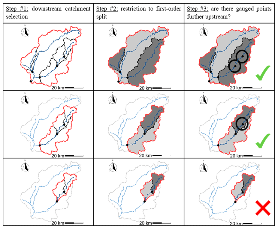
Figure 2 Illustration of the Matryoshka doll approach to the Vézère River at Larche. The steps of the method are shown in the columns and the discretization levels in the rows. From this initial catchment (top left), three semi-distributed configurations were obtained (number of rows). For each semi-distributed configuration, the boundary of the catchment considered is in red, the first-order upstream catchments are filled in dark grey, and the downstream catchment is in light grey.

The semi-distributed approach consists in performing lumped modelling in each sub-catchment by linking them through a hydraulic routing scheme. Thus, we need to distinguish between the first-order upstream catchment (Fig. 2, dark grey), where we applied a lumped rainfall–runoff model, and the downstream catchment (Fig. 2, light grey), where the rainfall–runoff model was applied after integrating the upstream inflows using a runoff-runoff model (hydraulic routing scheme). It is therefore important to differentiate between the routing part of hydrological models (enabling us to distribute the quantity of water contributing to the streamflow in the sub-catchment of interest, i.e. the intra-sub-catchment propagation, in time) and the hydraulic routing scheme (enabling us to propagate the streamflow simulated at one outlet to downstream catchment, i.e. the inter-sub-basin propagation). For this study, a single hydraulic routing scheme was applied. It is a time lag between the upstream and downstream outlet, as done by Lobligeois et al. (2014). In order to reduce the computation time, the authors propose calculating a lumped parameter C₀ corresponding to the average flow velocity over the downstream catchment. Since the hydraulic lengths d_i (i.e. the distance between the downstream outlet and each upstream sub-catchment) are known, the transit time T_i can be calculated as follows:

$$\begin{array}{}\text{(1)}& T_i={\displaystyle \frac{d_i}{C_{\mathrm{0}}}}.\end{array}$$

This approach is fairly simple but offers comparative performance to that of more complex routing models such as lag and route schemes (with linear or quadratic reservoirs) that account for peak-shaving phenomena (results not shown for the sake of brevity).

2.3 Models

In the context of this study, a model is defined as a configuration composed of a model structure and an associated set of parameters (i.e. which may vary according to the objective function selected for calibration). These models will be applied independently in a lumped or a semi-distributed modelling framework.

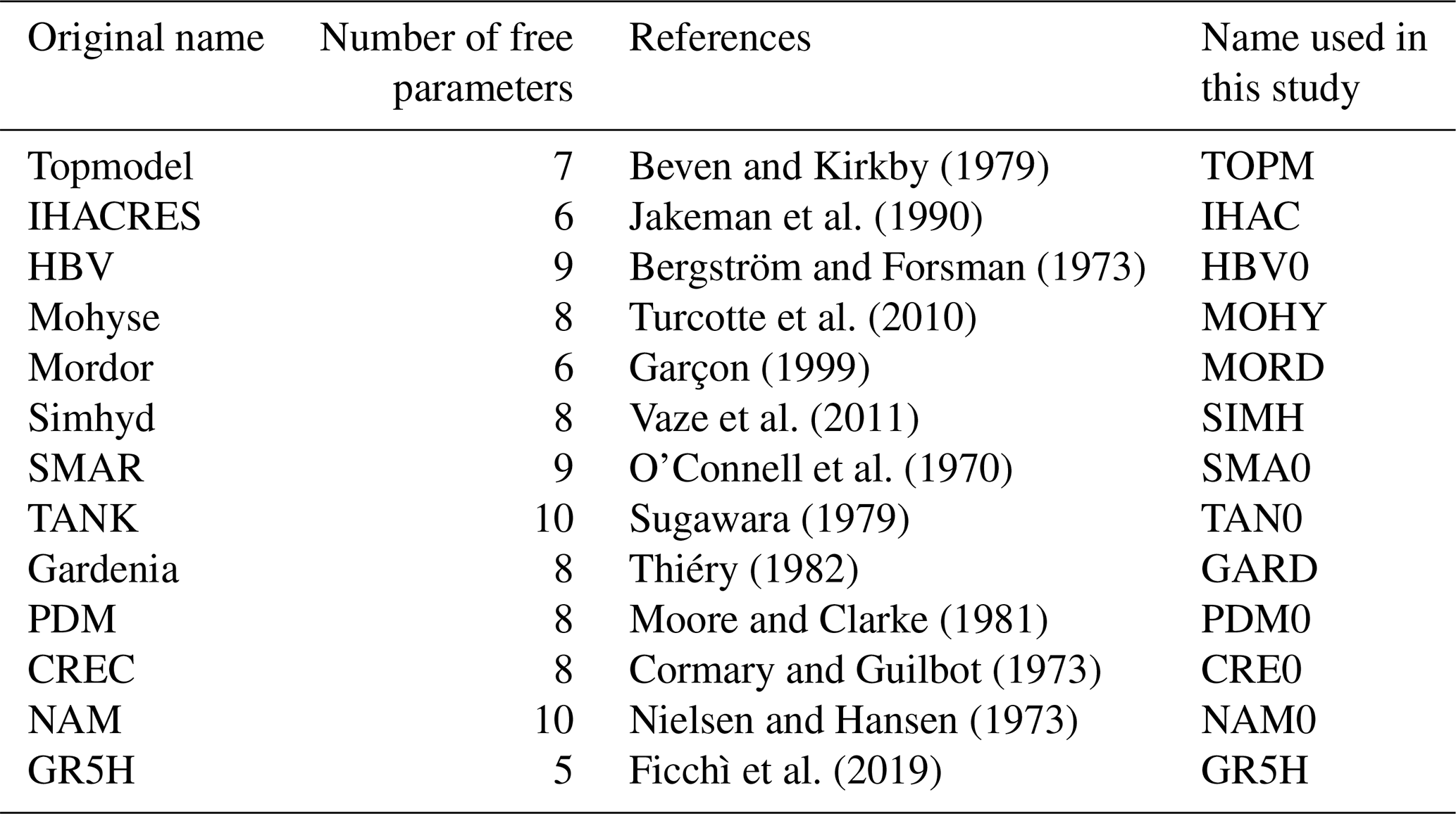
For this study, the airGRplus software (Coron et al., 2022), based on the works of Perrin (2000) and Mathevet (2005), was used. It includes various rainfall–runoff model structures running at the daily time step. airGRplus is an add-on to airGR (Coron et al., 2017, 2021). An adaptation of the work made by Perrin and Mathevet was carried out to use these structures at the hourly time step (mostly ensuring consistency of parameter ranges when changing simulation time steps and changing fixed time-dependent parameters). Finally, a set of 13 structures available in airGRplus, already widely tested in France and adapted to the hourly time step, was selected (Table 2). They are simplified versions of original rainfall–runoff models taken from the literature (except GR5H, which corresponds to the original version). To avoid confusion with the original models, a four-letter abbreviation was used here. Since the various catchments used for this study do not experience much snowfall, no snow module was implemented.

Table 2 List of rainfall–runoff models available in the airGRplus software at the hourly time step and used for this work.

The objective function used for parameter calibration is the Kling–Gupta efficiency (KGE) (Gupta et al., 2009), defined by

$$\begin{array}{}\text{(2)}& \mathrm{KGE}=\mathrm{1}-\sqrt{{\left(r-\mathrm{1}\right)}^{\mathrm{2}}+{\left(\mathit{\alpha }-\mathrm{1}\right)}^{\mathrm{2}}+(\mathit{\beta }-\mathrm{1}{)}^{\mathrm{2}}},\end{array}$$

with r the correlation, α the ratio between standard deviations, and β the ratio between the means (i.e. the bias) of the observed and simulated streamflow.

Thirel et al. (2023) showed that streamflow transformations are adapted to a specific modelling objective (e.g. low flows, floods). However, they highlighted that it is difficult to represent a wide range of streamflow with a single transformation. According to this study, we selected three transformations, two of which target high flows (Q^+0.5) and low flows (Q^−0.5), respectively, and one which is intermediate (Q^+0.1).

The algorithm used for model calibration comes from Michel (1991) and is available in the airGR package (Coron et al., 2017, 2021). It combines a global and a local optimization approach. First, a coarse screening of the parameters space is performed using either a rough predefined grid or a list of parameter sets. Then a steepest descent local search algorithm is performed, starting from the result of the screening procedure. Such calibration (over 10 years of hourly data) is about 0.5 to 6 min long (depending mainly of the catchment considered and the number of free parameters) and gives a single parameter set for a chosen objective function. Thus, we did not focus explicitly here on parameter uncertainty; i.e. we did not use multiple parameters sets for a single objective function as can be done with Monte Carlo simulations, for example. Such an approach would be interesting to consider as a perspective for this work but will not be covered here for computation time constraints. In a semi-distributed context, the calibration is carried out sequentially, i.e. in each sub-catchment from upstream to downstream. Note that the calibration takes slightly more time in the downstream catchment due to the additional free parameter of the routing function.

Overall, 13 structures and three objective functions were used, resulting in 39 models. Applied over two different spatial frameworks, a total of 78 distinct modelling options were available for this study.

2.4 Multi-model methodology

The multi-model approach consists in running various rainfall–runoff models. More specifically, here, we are interested in a deterministic combination of the different streamflow simulations. Let us recall that for our study, a model corresponds to the association of a structure and an objective function. By definition, a model is imperfect. Indeed, the different structures have been designed to meet different objectives (e.g. water resources management, forecasting, and climate change) in different geographical or geological contexts (e.g. high mountains, karstic zone, and alluvial plain). The objective functions (e.g. optimization algorithm, objective function, streamflow transformations), selected to optimize the parameters, are also choices that will eventually impact the simulation. The hypothesis made here is that the multi-model approach makes it possible to take advantage of the strengths of each model.

In the lumped framework, we consider every model in each catchment. In the semi-distributed framework, we consider every model in each sub-catchment. As the calibration is sequential, the various models are first applied to each upstream sub-catchment, and then their simulated streamflow is propagated to the downstream catchment to be modelled. However, transferring every upstream possibility to the downstream catchment is excessively time consuming. Therefore, the simulated streamflow in each upstream sub-catchment was first set with an a priori choice, whatever the model used, and then transferred to the downstream catchment (this choice is discussed in Sect. 4.4).

The multi-model framework enables these different streamflow simulations to be combined in each catchment and sub-catchment in order to create multiple additional simulations. At the downstream outlet, we will consider mixed combinations, using streamflow simulations from lumped and semi-distributed modelling (Fig. 3). To this end, deterministic averaging methods were used. Here, we will focus on a simple average combination (SAC), i.e. giving an equal weight to all models combined, defined by

$$\begin{array}{}\text{(3)}& Q_{\mathrm{SAC}}={\displaystyle \frac{{\sum }_{i=\mathrm{1}}^n{Q}_i}{n}},\end{array}$$

with Q_SAC the streamflow from a simple average combination and Q_i the simulated streamflow with a model i selected among the n models.

Note that a weighted average combination (WAC) was also tested but did not significantly change the mean results and was therefore not used further (discussed in Sect. 4.3).

The number of possible combinations on a given outlet from the total number of available streamflow simulations increases exponentially and can be computed by

$$\begin{array}{}\text{(4)}& n_{\mathrm{c}}=\sum _{i=\mathrm{2}}^{n_{\mathrm{sim}}}\left({\displaystyle \frac{n_{\mathrm{sim}}}{i}}\right),\end{array}$$

with i the number of streamflow simulations to choose from the total number of available streamflow simulations n_sim.

As an indication, there are approximately 1000 combinations for a streamflow ensemble simulated by 10 models, but there are over 1 000 000 solutions for 20 models in a lumped framework. Although a single combination is quick to perform (between 0.1 and 0.2 s), the number of combinations quickly becomes a limiting factor in terms of computation time. For this study, combinations will be set to a maximum of four different streamflow time series among the total number of models available, i.e. approximately 1 500 000 different combinations (discussed in Sect. 4.2):

$$\begin{array}{}\text{(5)}& n_{\mathrm{c}}=\sum _{i=\mathrm{2}}^{\mathrm{4}}\left({\displaystyle \frac{\mathrm{78}}{i}}\right)\approx \mathrm{1}\mathrm{500}\mathrm{000}.\end{array}$$

The objective of these combinations is to create a large set of simulations from which the best multi-model approach will be selected. Here we aim to obtain simulations that can perform well over a wide range of streamflow, and that can be applied to a large number of French catchments. Therefore, the best models (and multi-model approach) correspond to those which will achieve the highest performance in each catchment on average during the evaluation periods.

2.5 Testing methodology

A split-sample test (Klemeš, 1986), commonly used in hydrology, was implemented. This practice consists in separating a streamflow time series into two distinct periods, the first for calibration and the second for evaluation, and then exchanging these two periods. The two periods chosen are 1999–2008 and 2009–2018. An initialization period of at least 2 years was used before each test period to avoid errors attributable to the wrong estimation of initial conditions within the rainfall–runoff model.

For this study, results will only be analysed for evaluation (i.e. over the two untrained periods). Model performance was evaluated on two levels.

• With a general criterion. Model performance was evaluated with a composite criterion focusing on a wide range of streamflow, defined as follows:

  $$\begin{array}{}\text{(6)}& {\mathrm{KGE}}_{\mathrm{comp}}={\displaystyle \frac{\mathrm{KGE}\left(Q^{+\mathrm{0.5}}\right)+\mathrm{KGE}\left(Q^{+\mathrm{0.1}}\right)+\mathrm{KGE}\left(Q^{-\mathrm{0.5}}\right)}{\mathrm{3}}}.\end{array}$$

• With event-based criteria. Model performance was evaluated with several criteria characterizing flood and low flows. In a context of high flows (5447 events selected), the timing of the peak (i.e. the date at which the flood peak was reached), the flood peak (i.e. the maximum streamflow value observed during the flood) and the flood flow (i.e. mean streamflow during the event) were analysed. In a context of low flows (1332 events selected), the annual low-flow duration (i.e. number of low-flow days) and severity (i.e. largest cumulative streamflow deficit) were studied. Table 3 provides typical ranges of values of flood and low-flow characteristics over the catchment set. Please refer to Appendix A and B for more details on the event selection method.

Table 3 Minimum, median, and maximum values of flood and low-flow characteristics over the 121 catchments.

In a multi-model framework, the best (i.e. giving the best performance over the evaluation periods) model or combination of models for each catchment can be determined. Therefore, this model or combination of models will differ from one catchment to another. For this work we chose as a benchmark a lumped one-size-fits-all model (i.e. the same model whatever the catchment), which is the hydrological modelling approach usually used.

3 Results

Results are presented from lumped (L) single models (SMs), i.e. run individually, to more complex semi-distributed (SD) multi-model (MM) approaches (see Fig. 3). The mixed (M) multi-model approach allows for a variable spatial framework combining both lumped and semi-distributed approaches. The aim of this section is to present the results obtained with each modelling framework and their intercomparison.

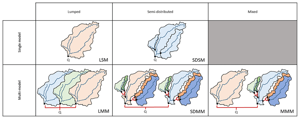
Figure 3 Summary of the different approaches tested. Q is the target streamflow at the main catchment outlet; black dots show gauging stations used. The different colours represent different model structures. The variations of the same colour indicate different parameterizations. Red links represent the combination of streamflow.

3.1 Lumped single models (LSMs)

In this part, each model was run individually in a lumped mode (see Fig. 3). Parameters of the 13 structures were calibrated successively with the three objective functions, resulting in 39 lumped models.

Figure 4 shows the distribution of the performance of lumped single models over the 121 downstream outlets and over the evaluation periods. As a reminder, the KGE_comp used for the evaluation is a composite criterion which considers different transformations in order to provide an overall picture of model performance for a wide range of streamflow (Eq. 6). Overall, lumped single models give median KGE_comp values between 0.70 and 0.88. This upper value is reached with the GR5H structure calibrated with a generalist objective function (KGE applied to Q^+0.1) and will be used in the paper as a benchmark. Since efficiency criteria values depend on the variety of errors found in the evaluation period (see, for example, Berthet et al., 2010), this may impact the significance of performance differences between models and ultimately their comparison. Therefore, we tried to quantify the sampling uncertainty in KGE scores. The bootstrap–jackknife methodology proposed by Clark et al. (2021) was applied over our sample of 121 catchments for the 39 lumped models. It showed a median sampling uncertainty in KGE scores of 0.02 (Appendix C). The objective function applied during the calibration phase seems to have a variable impact on performance depending on the structure. For example, GR5H shows a similar performance regardless of the transformation applied, whereas TAN0 shows a large variation. The strong decrease in the 25 % quantile of the latter is linked to the great difficulty for this structure to represent the low-flow component of KGE_comp when it is calibrated with more weight on high flows (KGE applied to Q^+0.5). The reverse is also true since a structure optimized with more weight on low flows (KGE applied to Q^−0.5) will have more difficulties to represent the high-flow component of KGE_comp (e.g. NAM0 or GARD). Although the differences remain limited, the highest KGE_comp scores are achieved with a more generalist objective function (KGE applied to Q^+0.1). These results confirm the conclusions reached by Thirel et al. (2023).

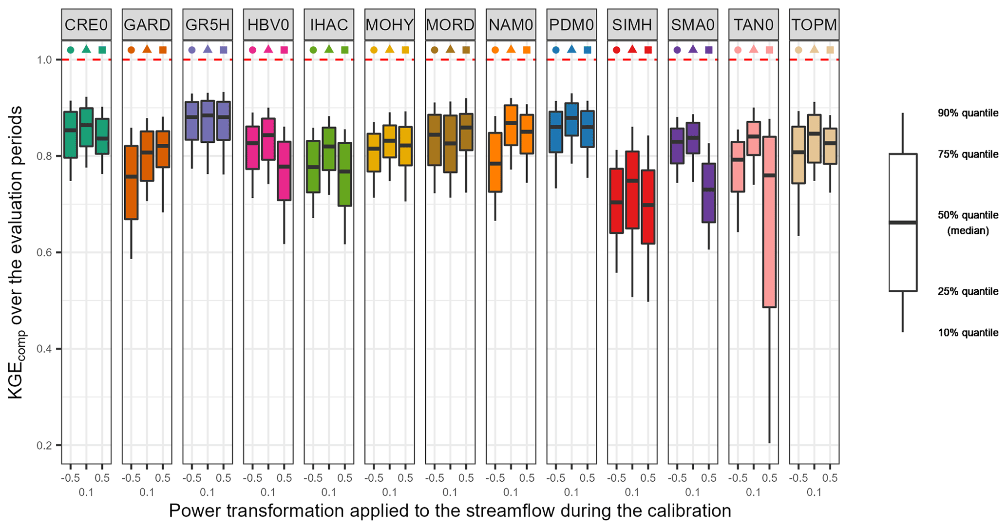
Figure 4 Distribution of the performance (KGE_comp score) of the 39 lumped single models over the 121 catchments and over the evaluation periods. The box plots represent the 10 %, 25 %, 50 %, 75 % and 90 % quantiles. The dashed red line represents the optimal KGE value. Each colour represents a structure, and each geometric pattern represents the power transformation applied to the streamflow during the calibration.

The left part of Fig. 5 highlights the results obtained by selecting the best lumped single model in each catchment (LSM). In this modelling framework, the median KGE_comp is 0.91 (0.03 higher than the one-size-fits-all model used as a benchmark) with low variation (between 0.88 and 0.93 for the 25 % and 75 % quantiles). The right part of Fig. 5 indicates the number of catchments where each lumped single model is defined as the best. As expected, the models with high performance over the whole sample are selected more often than the others. However, two-thirds of the lumped single models have been selected at least once as the best in a catchment. Similar results can be found in Perrin et al. (2001) or Knoben et al. (2020).

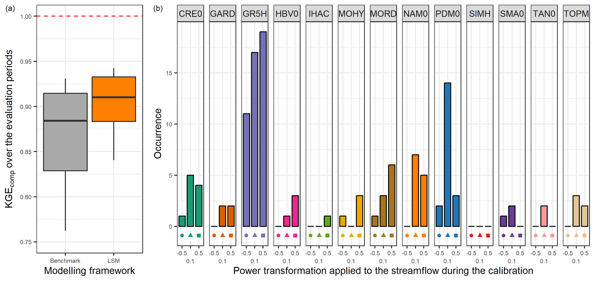
Figure 5 Distribution of the performance (KGE_comp score) of the best lumped single models (LSMs) over the 121 catchments (a) and model occurrence within this selection (b). The box plots represent the 10 %, 25 %, 50 %, 75 %, and 90 % quantiles. The dashed red line represents the optimal KGE value. The benchmark corresponds to a one-size-fits-all approach, with the GR5H structure calibrated with a generalist objective function Q^+0.1 over the whole catchment set.

3.2 Semi-distributed single models (SDSMs)

Remember that the semi-distribution with a single model (see Fig. 3) is done sequentially, i.e. from upstream to downstream. Thus, each upstream sub-catchment is first modelled in a lumped mode with a single structure–objective function pair. Then, the streamflow simulated upstream is propagated and the same model is calibrated and applied to the downstream catchment. This procedure is repeated for all 39 (13 structures and three objective functions) available models.

Figure 6 shows the difference between KGE_comp values obtained with lumped single models and semi-distributed single models. The semi-distributed approach seems to have a positive overall impact on the performance, although some deterioration can also be observed. Overall, the differences are limited (median of 0.02). However, the semi-distributed approach seems to have a variable impact on performance depending on the structure. For example, CRE0 shows a similar performance regardless of the spatial framework applied, whereas the performance of GARD improved with a spatial division. Although there is no clear trend in the impact of the semi-distribution in relation to the transformation applied during calibration, it seems that models calibrated on Q^+0.1 (i.e. giving “equal” weight on all flow ranges) show lower differences. The lumped models with the highest performance seem to benefit less (if any) from semi-distribution. On the other hand, lumped models with lower performance seem to benefit from the spatial discretization.

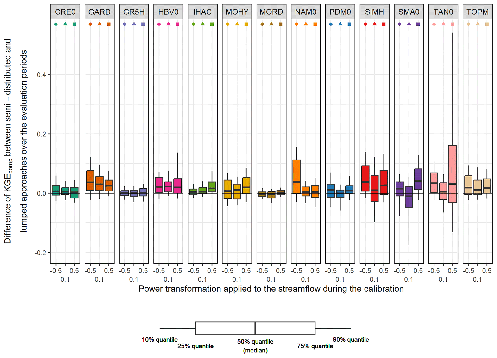
Figure 6 Comparison of the performance (KGE_comp score) between lumped and semi-distributed single models over the 121 catchments and over the evaluation periods. The box plots represent the 10 %, 25 %, 50 %, 75 %, and 90 % quantiles. Each colour represents a structure, and each geometric pattern represents the power transformation applied to the streamflow during the calibration. The black line indicates an equal performance between the lumped and semi-distributed approaches; the upper part indicates an increase of performance with the semi-distributed approach (and the lower part a decrease).

Nevertheless, Fig. 7 highlights that overall, if the focus is set on the best model in each catchment, the difference between the semi-distributed and lumped single model remains small (no deviation for the quartiles and only 0.005 for the median). Once again, two-thirds of the semi-distributed single models have been selected at least once as the best in a catchment.

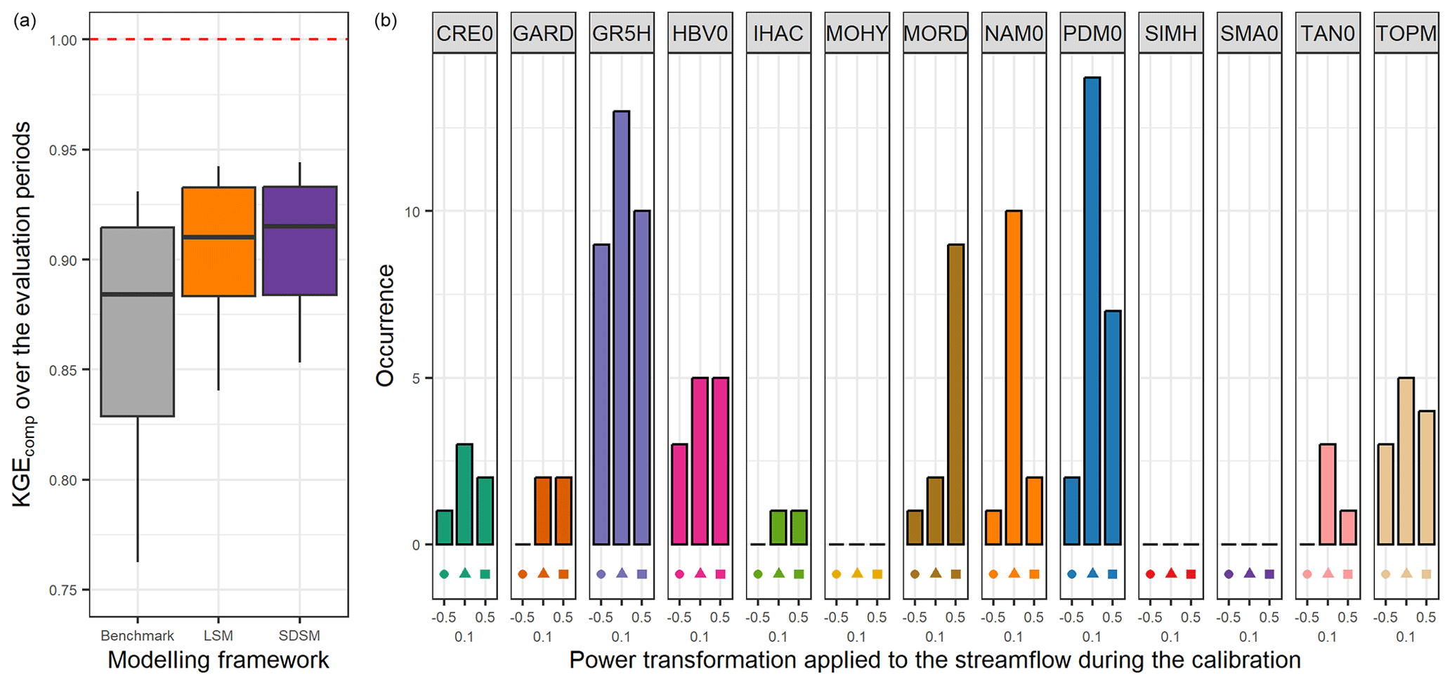
Figure 7 Distribution of the performance (KGE_comp score) of the best semi-distributed single models (SDSMs) over the 121 catchments (a) and model occurrence within this selection (b). The box plots represent the 10 %, 25 %, 50 %, 75 %, and 90 % quantiles. The dashed red line represents the optimal KGE value. The benchmark corresponds to a one-size-fits-all approach, with the GR5H structure calibrated with a generalist objective function Q^+0.1 over the whole catchment set.

3.3 Lumped multi-model (LMM) approach

Here, each model was run in a lumped mode, and model outputs were combined (see Fig. 3). The multi-model approach used in this work is a deterministic combination with simple average (SAC) and will be limited to a combination of a maximum of four models among the available lumped models, i.e. approximately 92 000 different combinations.

The left part of Fig. 8 shows the comparison between performance obtained with the benchmark and when the best lumped multi-model approach is selected in each catchment. The combination of lumped models enables an increase of 0.06 in the median KGE_comp value compared with the benchmark and of 0.03 compared with the LSM approach. While this gain may seem small at first glance, it is quite substantial since the performance obtained with the benchmark was already very high (median of 0.88), which makes improvements increasingly difficult. The right part of Fig. 8 shows the number of times each model is selected within the best-performing multi-model approach. As expected, it highlights the benefits of a wide choice of models (similar results were found by Winter and Nychka, 2010). Indeed, even if some of the models had never been used for the benchmark simulation (in a lumped single-model framework), the multi-model approach shows that each of them can become a contributing factor to improve streamflow simulation in at least one catchment. Moreover, the models that are most often selected in the model combinations are not always the best models on their own. For example, TOPM, calibrated to favour high flows (Q^+0.5), was only used in the benchmark on 1.5 % of the catchments but it is selected in the multi-model approach on 24 % of the catchments. However, the converse does not seem to be true since a model with good individual performance always seems to be a key element of the multi-model approach (e.g. GR5H, PDM0, MORD).

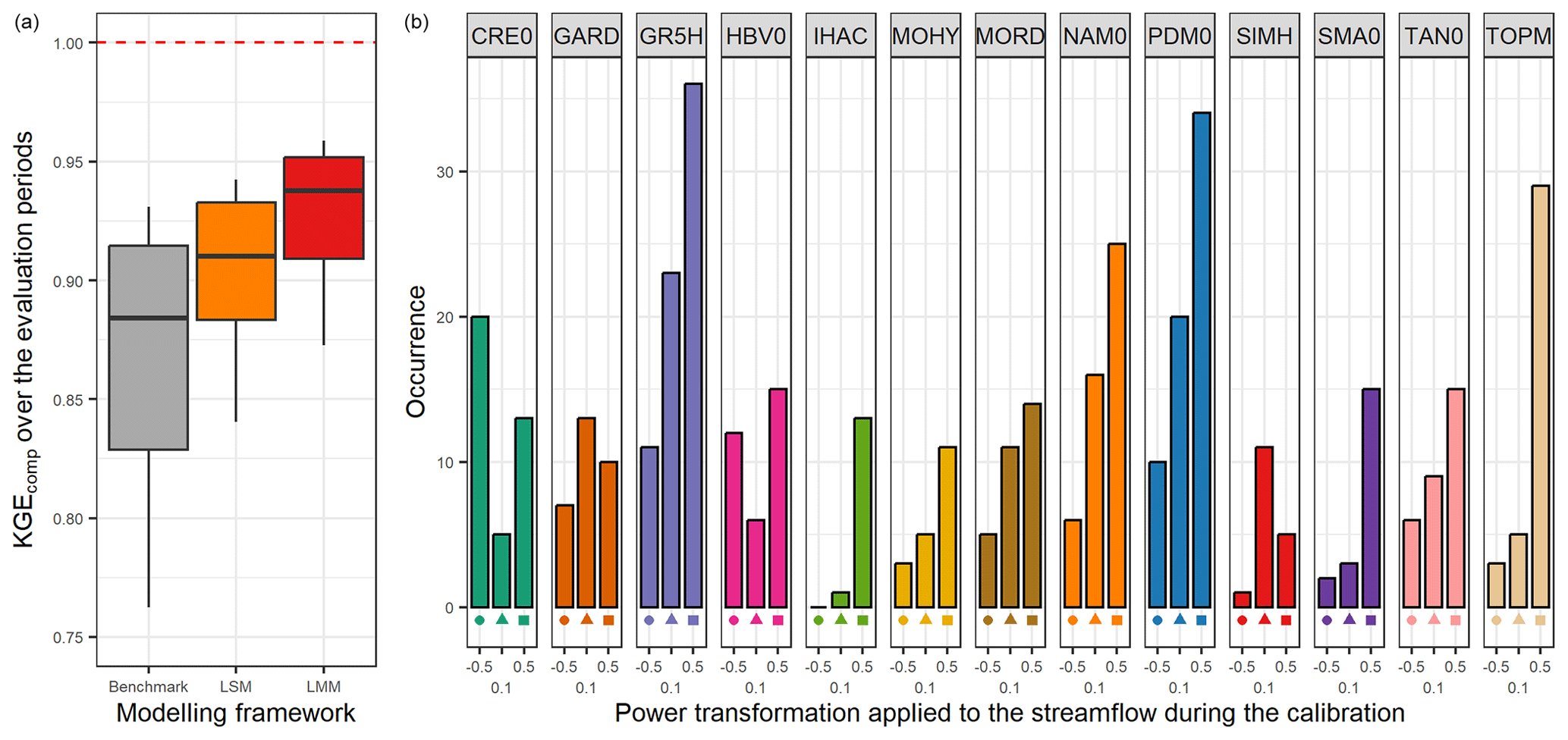
Figure 8 Distribution of the performance (KGE_comp score) of the best lumped multi-model (LMM) approach over the 121 catchments (a) and model occurrence within this selection (b). The box plots represent the 10 %, 25 %, 50 %, 75 %, and 90 % quantiles. The dashed red line represents the optimal KGE value. The benchmark corresponds to a one-size-fits-all approach, with the GR5H structure calibrated with a generalist objective function Q^+0.1 over the whole catchment set.

3.4 Semi-distributed multi-model (SDMM) approach

For this study, the semi-distributed multi-model approach (see Fig. 3) of the target catchment is performed in two steps. First, the best multi-model combination (i.e. the combination of two to four models among the 39 available giving the highest performance over the evaluation periods) in each upstream sub-catchment is identified. In the second step, the simulated mean upstream streamflow is propagated downstream, and the different models are applied and then combined (by two, three, or four) on the downstream catchment. Thus, approximately 92 000 different possible combinations of simulated streamflow are obtained at the outlet of the total catchment.

Figure 9 shows very similar results to the LMM (Sect. 3.3). Indeed, we find again an improvement in the median of 0.06 compared to the benchmark, and all the models are used on at least one downstream catchment. Moreover, the distribution of the model count on the downstream catchment seems to be more homogeneous between the different members.

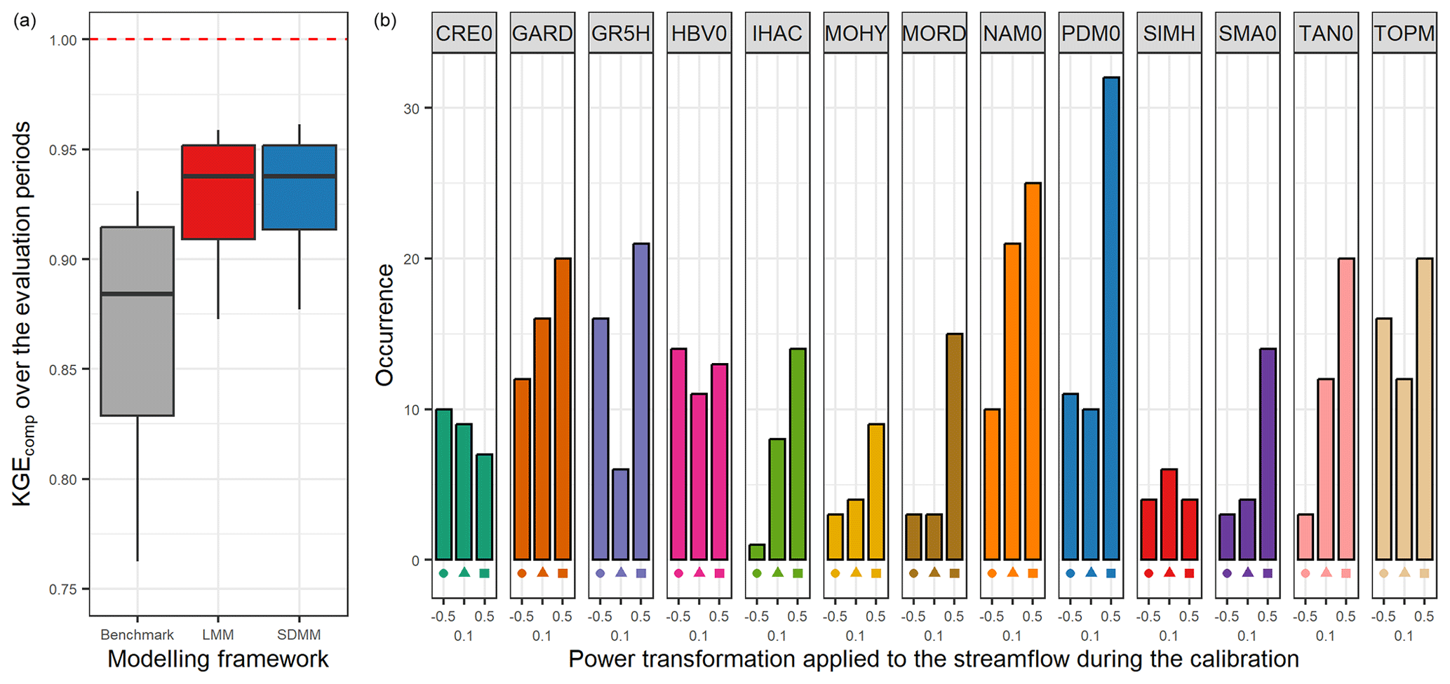
Figure 9 Distribution of the performance (KGE_comp score) of the best semi-distributed multi-model (SDMM) approach over the 121 catchments (a) and model counts on the downstream catchment within this selection (b). The box plots represent the 10 %, 25 %, 50 %, 75 %, and 90 % quantiles. The dashed red line represents the optimal KGE value. The benchmark corresponds to a one-size-fits-all approach, with the GR5H structure calibrated with a generalist objective function Q^+0.1 over the whole catchment set.

3.5 Mixed multi-model (MMM) approach

Here, the mixed multi-model approach represents a combination of all the approaches tested above. This method allows a combination of models for a variable spatial framework (see Fig. 3) for each catchment. In this context, the 39 models applied to a lumped and a semi-distributed framework are used, resulting in 78 modelling options, each giving a different streamflow at the outlet (Fig. 10). These simulations can then be combined (by two, three, or four) downstream in order to define the best mixed multi-model approach in each catchment among more than 1 500 000 possibilities.

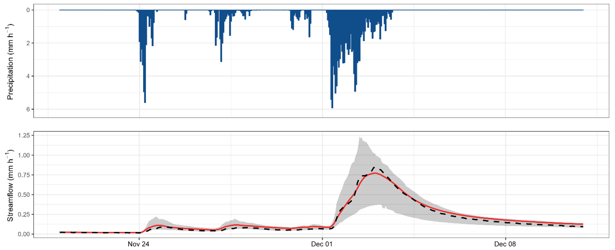
Figure 10 Hydrograph of November–December 2003 of the Dore River at Saint-Gervais-sous-Meymont (K287191001). The grey shading shows the interval between the 10 % and 90 % quantiles generated by the 78 modelling options. The red line highlights the best MMM combination. The dashed black line refers to the observed streamflow.

The left part of Fig. 11 shows the performance obtained with the best mixed multi-model approach. The combination of lumped and semi-distributed models outperforms the benchmark, but results are still close to those obtained using the LMM or SDMM approaches. The right part of Fig. 11 highlights the benefits gained from the wide choice of models and a variable spatial framework. Indeed, almost every lumped and semi-distributed model is used in order to improve the representation of streamflow with a multi-model approach in at least one catchment.

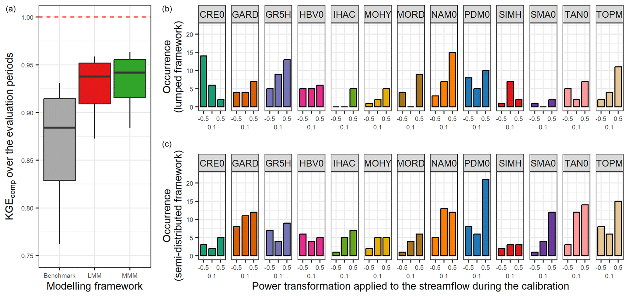
Figure 11 Distribution of the performance (KGE_comp score) of the best mixed multi-model approach over the 121 catchments (a) and model counts within this selection (b). The box plots represent the 10 %, 25 %, 50 %, 75 %, and 90 % quantiles. The dashed red line represents the optimal KGE value. The benchmark corresponds to a one-size-fits-all approach, with the GR5H structure calibrated with a generalist objective function Q^+0.1 over the whole catchment set.

3.6 Modelling framework comparison

Figure 12 compares the performance obtained when the best (multi-)model is selected in each catchment depending on the modelling approach used. First, all approaches tested outperform the benchmark. Then, the best LSM and SDSM distributions are almost identical, and the same results are obtained with LMM and SDMM. This shows a limited gain of the semi-distribution approach compared to a lumped framework. However, the LMM and SDMM outperformed the LSM and SDSM. Therefore, the increase in performance is mainly due to the multi-model aspect. Finally, the highest performance is obtained with the MMM, but it remains close to the performance achieved by the LMM and SDMM.

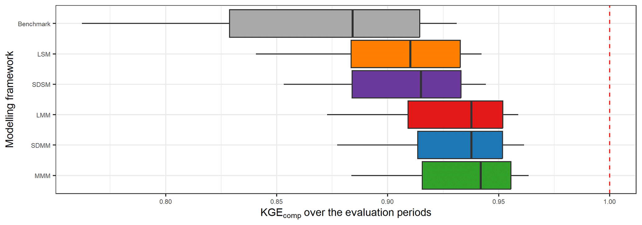
Figure 12 Distribution of the performance (KGE_comp score) of the best (multi-)models over the 121 catchments according to their modelling framework (LSM – lumped single-model, SDSM – semi-distributed single-model, LMM – lumped multi-model, SDMM – semi-distributed multi-model, MMM – mixed multi-model). The dashed red line represents the optimal KGE value. The benchmark corresponds to a one-size-fits-all approach, with the GR5H structure calibrated with a generalist objective function Q^+0.1 over the whole catchment set.

Figure 13 shows the best-performing modelling framework for each catchment. Multi-model approaches are considered to be better than single models for the vast majority of catchments. In general, the MMM approach seems to be the most suitable for most of the catchments. However, if we accept to deviate by 0.005 (epsilon value arbitrarily set) from the optimal value, we notice that the lumped multi-model approach is sufficient on a large part (about 60 %) of the catchments. There are no clear regional trends on which catchments require a more complex modelling framework.

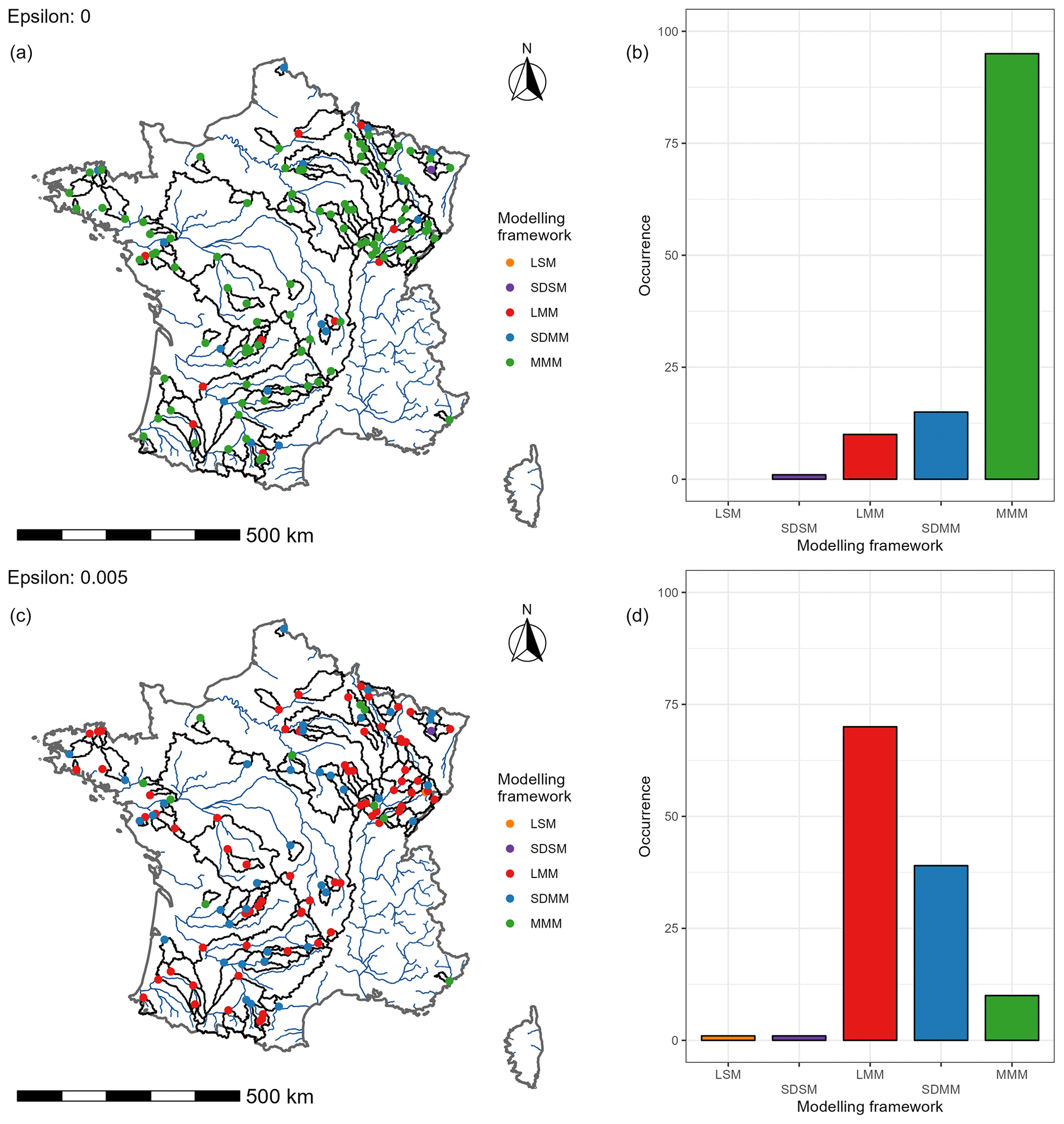
Figure 13 Maps of the best modelling framework in each catchment (a–b) and the simplest modelling framework among the best frameworks (c–d). The epsilon value corresponds to the performance deviation allowed from the best performance. If the drop between the evaluation performances is lower than or equal to epsilon, then the simplest modelling framework is selected.

Figure 14 shows the evaluation of the different modelling frameworks at the event scale. As a reminder, only the best (multi) model in each catchment is analysed for each approach tested. Typical ranges of values of flood and low-flow characteristics over the catchment set are provided Table 3.

The flood peak is late by about 1 h for the single-model approaches, whereas with a multi-model framework, it comes 1 h too early. The most extreme values correspond to large catchments with slow responses and a strong base flow impact. In addition, multi-model approaches seem to have a lower variability for this criterion. The peak flow is slightly underestimated with a median of −0.05 mm h⁻¹, like the flood flow, which shows a median deficit of 0.02 mm h⁻¹. There does not seem to be a clear trend in the contribution of a complex mixed multi-model approach compared to a lumped single model (benchmark).

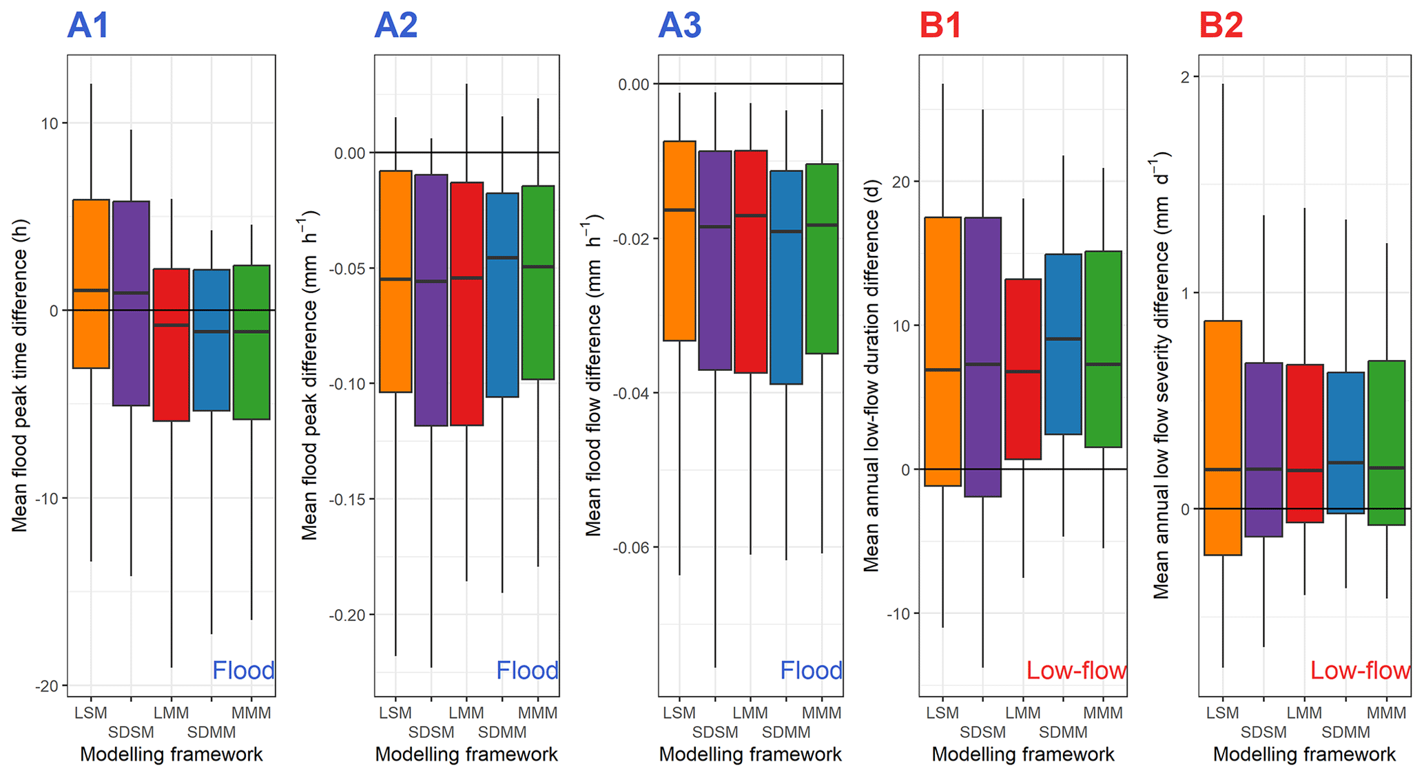
Figure 14 Comparison of various criteria between simulated and observed flood (A1, A2, and A3) or low-flow (B1 and B2) events, according to the modelling approach used. The box plots represent the 10 %, 25 %, 50 %, 75 %, and 90 % quantiles. The black line indicates the equivalence between the observed and simulated criteria. A positive value indicates an overestimation of the criterion by the simulation compared to observed streamflow.

4 Discussion

Here, the first objective is to discuss the results and answer the initial question: what is the possible contribution of a multi-model approach within a variable spatial framework for the simulation of streamflow over a large set of catchments? The second objective is to discuss the methodological choices by analysing them independently to determine to what extent they impact the results.

4.1 What is the possible contribution of a multi-model approach within a variable spatial framework?

First, our results confirmed the findings previously reported in the literature. Indeed, the multi-model approach outperformed the single models for a large sample of catchments (Shamseldin et al., 1997; Georgakakos et al., 2004; Ajami et al., 2006; Winter and Nychka, 2010; Velázquez et al., 2011; Fenicia et al., 2011; Santos, 2018; Wan et al., 2021). Moreover, there is no clear benefit (on average) of using a semi-distributed framework because it degrades the streamflow simulation in some catchments and improves it in others (Khakbaz et al., 2012; Lobligeois et al., 2014; de Lavenne et al., 2016).

The originality of our study is to combine these two approaches while providing a variable spatial framework. The mixed multi-model approach thus seems to benefit from the strengths of both methods. Most of the improvements compared to our benchmark come from the multi-model approach. On the other hand, although for a large part of the sample the differences are negligible, the variable spatial framework seems to generate an increase in the mean KGE values of up to 0.03 compared to a lumped multi-model approach (Fig. 15). It should be noted that a similar difference is observed for the single models. By design, the MMM does not deteriorate the performance when compared to what can be initially obtained with the LMM and SDMM approaches.

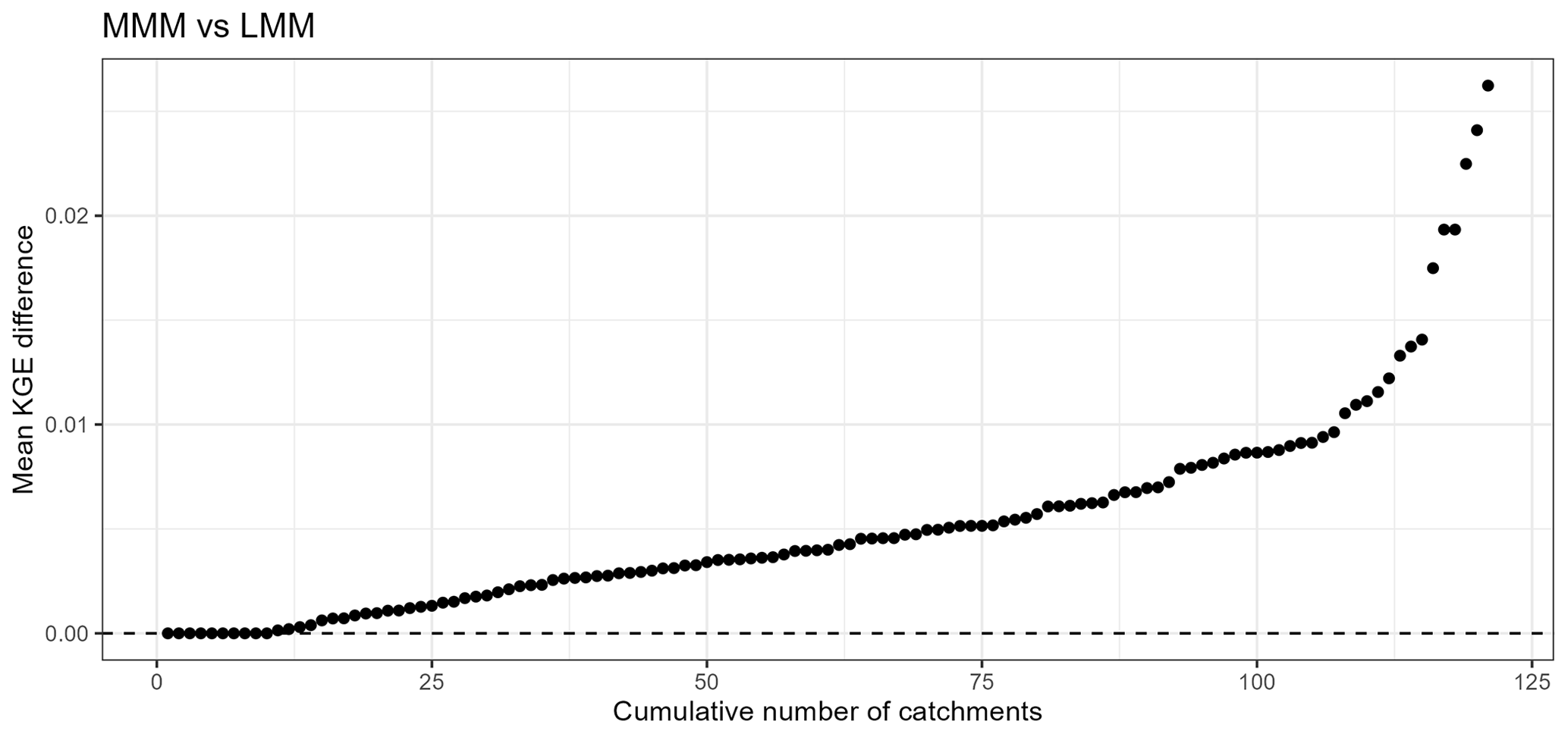
Figure 15 Ranked performance difference curve obtained for the evaluation periods between the best lumped and mixed multi-model approach in each catchment. The black line indicates the equivalence between the two modelling frameworks. The higher the value, the greater the benefit of a variable spatial framework.

Generally, this study has shown that a large number of models enables a better performance regardless of the streamflow range over a large sample of catchments. However, this methodology can be computationally expensive (due to the exponential number of combinations).

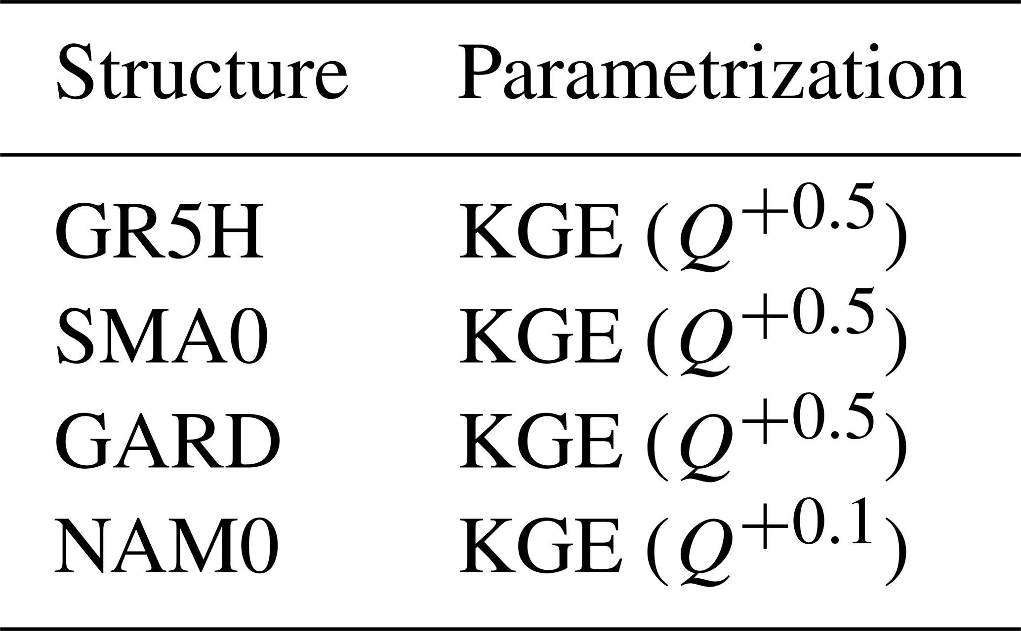
Winter and Nychka (2010) showed that in a multi-model framework, a key point is not only the number of models but also their differences. However, it is difficult to quantify explicitly this difference a priori. Various configurations of small pools of four models (i.e. structure–objective function pairs) were tested before selecting only the best of them (called “simplified MMM”; see Table 4 for more details). A mixed multi-model test was performed over this sample in order to reduce the complexity brought about by a large number of models.

As a reminder, the procedure is the following:

• In a semi-distributed framework, each of the four lumped models was applied and then combined for each upstream sub-catchment of the sample. Then, the best combination (i.e. giving the highest KGE value over the evaluation periods) at each upstream outlet was propagated through the downstream catchment where the subsample of models was also used.

• In a lumped framework, the modelling of each total catchment was performed with the different members of the simplified MMM.

• Downstream simulations (four from the lumped approach and four from the semi-distributed approach) were then combined (resulting in 162 combinations), and the best multi-model combination at the outlet was selected.

Figure 16 shows that with the simplified MMM, the multi-model approach in a variable framework gives better KGE values than the LSM approach (which uses each lumped model independently and then selects the best one in each catchment). However, the performance obtained with the MMM approach is not reached, which again shows the added value of a wide choice of models.

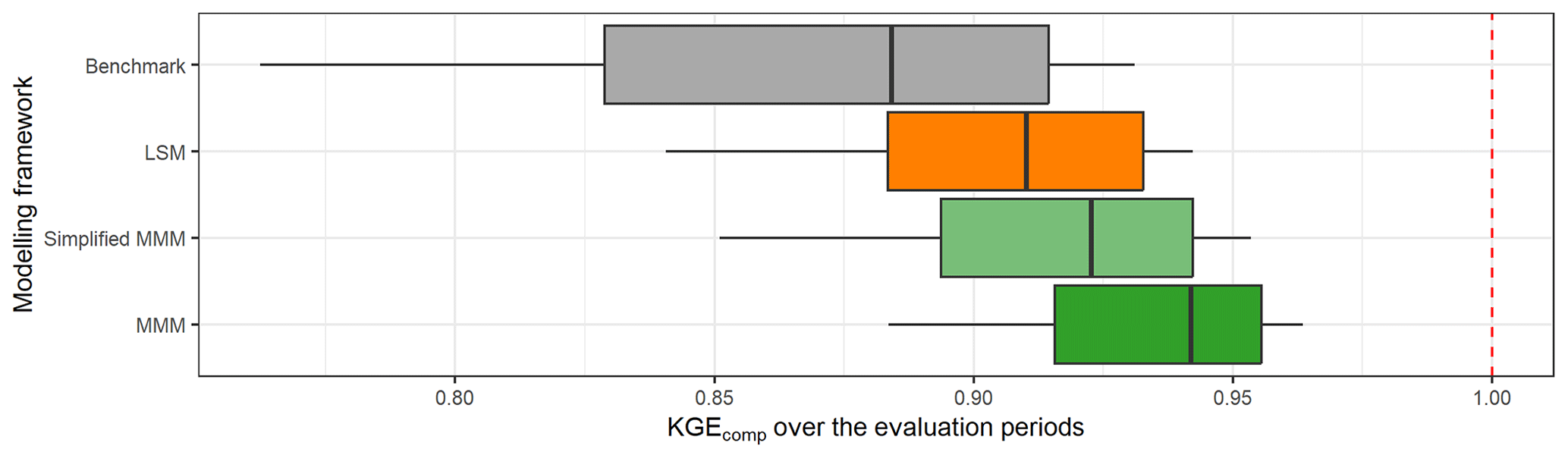
Figure 16 Distribution of the best simplified mixed multi-model approach, defined with a subset of four models, over the entire sample of catchments and over the evaluation periods. The box plots represent the 10 %, 25 %, 50 %, 75 %, and 90 % quantiles. The dashed red line represents the optimal KGE value. The benchmark corresponds to a one-size-fits-all approach, with the GR5H structure calibrated with a generalist objective function Q^+0.1 over the whole catchment set.

Table 4 Composition of the simplified MMM.

4.2 What is the optimal number of models to combine in a multi-model framework?

The optimal number of models to combine in a multi-model framework varies between past studies. For example, Wan et al. (2021) found that a limited improvement is achieved when more than nine models are combined, Arsenault et al. (2015) concluded that seven models were sufficient, and Kumar et al. (2015) highlighted a combination of five members. This optimal number therefore seems to vary with the catchment sample but also according to the number of models used and their qualities. Figure 17 shows the results obtained by the best lumped (multi-)model in each catchment according to the number of members combined. The largest improvement comes from a simple combination of two models, and the performance gain becomes limited from a combination of four different models (at least in our study).

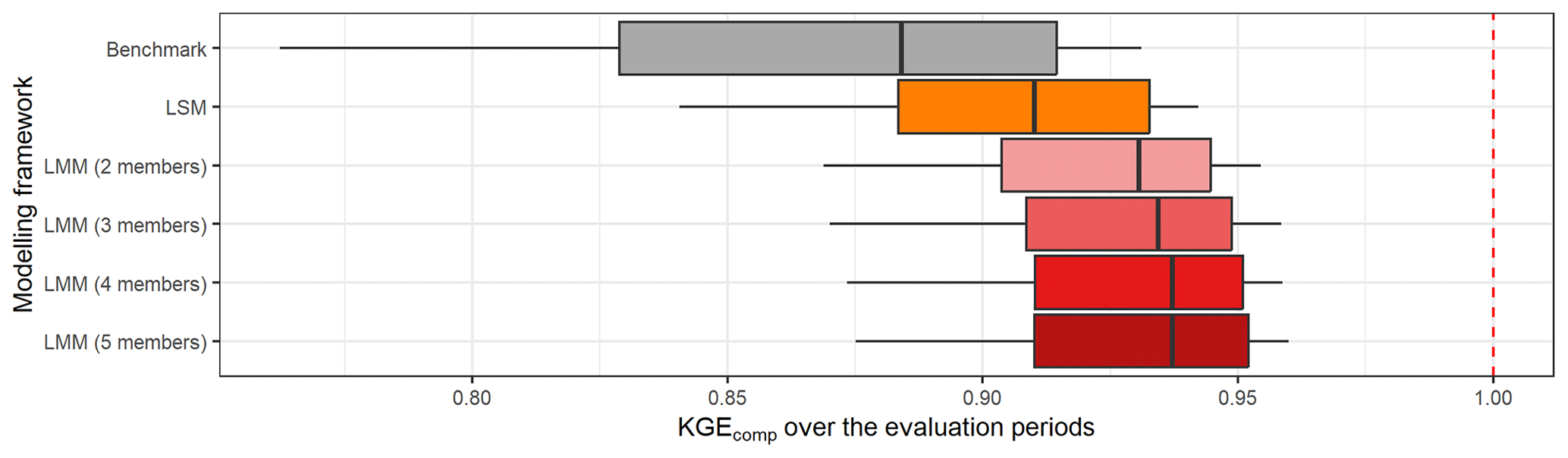
Figure 17 Distribution of the performance obtained with the best lumped multi-model approach in each catchment according to the number of models combined. The box plots represent the 10 %, 25 %, 50 %, 75 %, and 90 % quantiles. The dashed red line represents the optimal KGE value. The benchmark corresponds to a one-size-fits-all approach, with the GR5H structure calibrated with a generalist objective function Q^+0.1 over the whole catchment set.

4.3 Is a weighted average combination always better than a simple average approach?

The weighted average combination (WAC) consists of assigning a weight that can be different for each model (Eq. 4), as opposed to the simple average combination (SAC), which considers each model in an identical manner (Eq. 3).

$$\begin{array}{}\text{(7)}& Q_{\mathrm{WAC}}={\displaystyle \frac{{\sum }_{i=\mathrm{1}}^n{\mathit{\alpha }}_i.Q_i}{{\sum }_{i=\mathrm{1}}^n{\mathit{\alpha }}_i}},\end{array}$$

with Q_WAC the streamflow from a weighted average combination, Q_i the simulated streamflow with a model i selected among the n models, and α_i its attributed weight (between 0 and 1).

The complexity of the weighted average procedure lies in the estimation of the weights. Here, the weights have been optimized according to the capacity of the combination to represent the observed streamflow by maximizing the KGE on the transformations chosen during the calibration of the models. Thus, we obtain a set of weights for each calibration criterion used by testing all possible values in steps of 0.1 between 0 and 1. The average of these different weight sets for the three objective functions will then be taken as the final weighting.

This method becomes very expensive in terms of calculation time when the number of models increases. Thus, to answer this question, a subsample of 13 models (corresponding to the 13 structures calculated on the square root of streamflow in a lumped framework) was selected, and the tests were limited to a combination of three models (representing 364 distinct combinations in total).

Figure 18 shows the comparison of the SAC and WAC methods. Each point represents the mean KGE obtained over the evaluation periods by each combination of models over the whole sample of catchments and over all the transformations evaluated. It highlights that the WAC and SAC methods provide similar mean results when dealing with a wide range of streamflow.

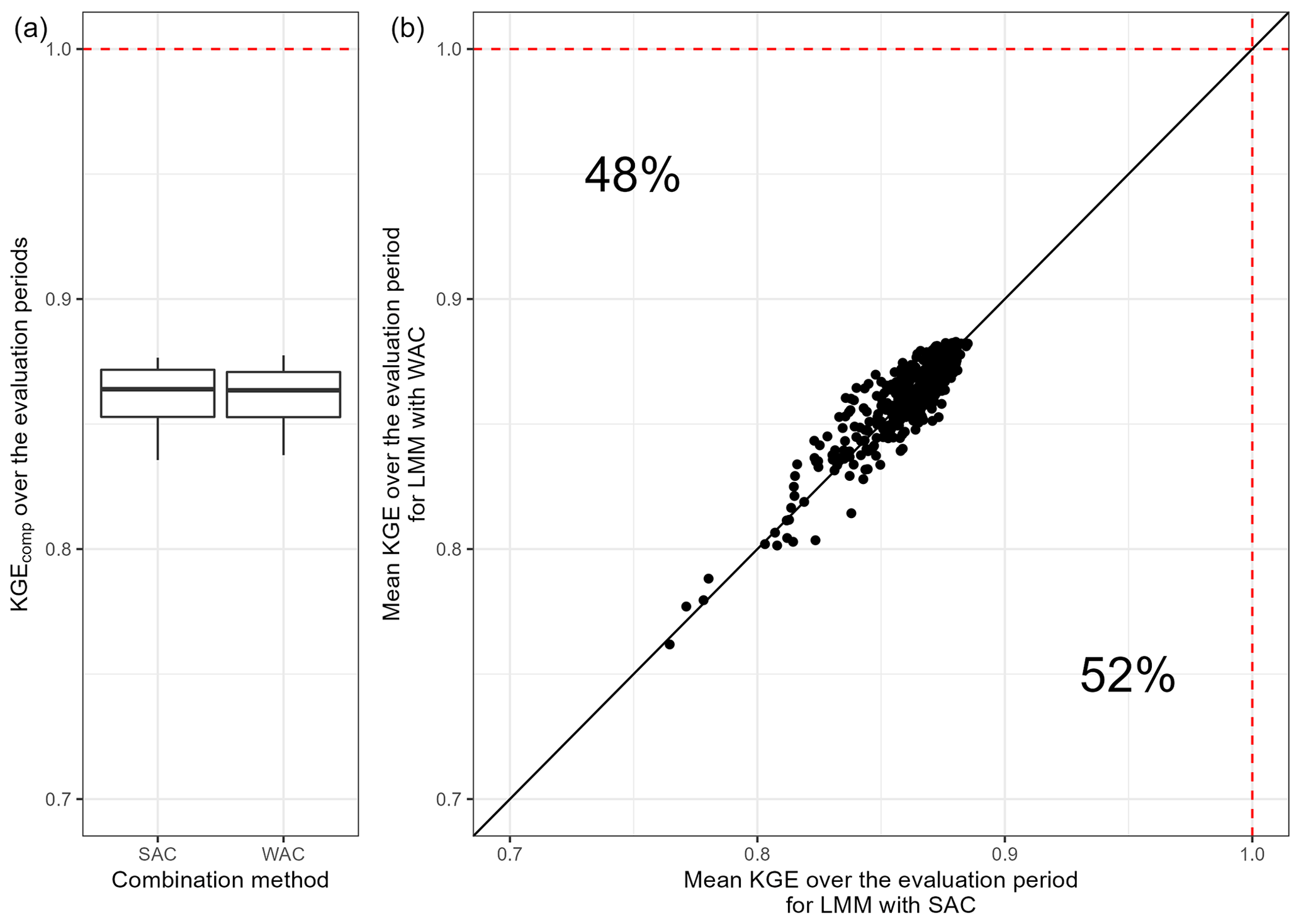
Figure 18 Comparison of the performance obtained over the evaluation periods by each multi-model approach for the whole catchment sample according to the combination method used. The box plots represent the 10 %, 25 %, 50 %, 75 %, and 90 % quantiles. The dashed red line represents the optimal KGE value. The black line indicates the equivalence between the two combination methods.

Another limit of the WAC procedure lies in the variability of the coefficients according to the calibration period. Moreover, this instability seems to increase with the number of models used in the combinations.

Is the a priori choice to use the best upstream multi-model approach always justified?

As a reminder, semi-distribution consists in dividing a catchment into several sub-catchments which can then be modelled individually with their own climate forcing and parameters and then linked together by a propagation function. Generally, the number of possible streamflow simulations in a catchment is set as

$$\begin{array}{}\text{(8)}& n=n_{\mathrm{sim}}+n_{\mathrm{c}}\left(n_{\mathrm{sim}}\right),\end{array}$$

with n_sim the number of simulations available and n_c the number of combinations from n_sim.

However, the number of simulations in a semi-distributed framework depends on the number of models available in this catchment and increases rapidly with the streamflow simulations injected from upstream catchments.

$$\begin{array}{}\text{(9)}& \begin{array}{ll}{n}_{\mathrm{sim}}=n_{\mathrm{mod}}\times \prod _{i=\mathrm{1}}^x{n}_{{\mathrm{up}}_i}& \mathrm{if}x>\mathrm{0}\\ n_{\mathrm{sims}}=n_{\mathrm{mod}}& \mathrm{if}x=\mathrm{0},\end{array}\end{array}$$

with n_mod the number of available models on the sub-catchment considered, x the number of direct upstream sub-catchments, and $n_{{\mathrm{up}}_i}$ the number of possible streamflow available at the outlet of the upstream sub-catchment i.

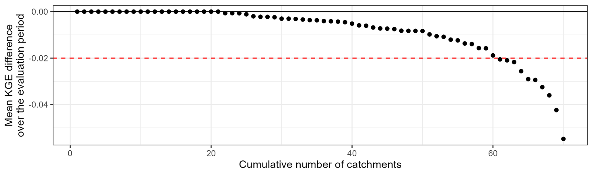
Figure 19 Ranked performance difference curve obtained for the evaluation periods in each catchment by the best downstream model with an a priori choice on upstream simulation or not. The black line indicates the equivalence between the modelling frameworks. A negative value indicates a decline in performance due to the a priori choice of upstream simulations injected.

It is therefore necessary to make an a priori choice on the different upstream sub-catchments in order to reduce the number of possibilities downstream. The assumption made in this study is to propagate a single simulation, resulting from the best combination of models, for each sub-catchment. Equation (8) then becomes

$$\begin{array}{}\text{(10)}& n=n_{\mathrm{mod}}+n_{\mathrm{c}}\left(n_{\mathrm{mod}}\right).\end{array}$$

This hypothesis ensures the same number of downstream streamflow simulations in a lumped or semi-distributed modelling framework (as complex as it can be).

Simplified tests (semi-distributed configurations with one upstream catchment – i.e. 70 catchments – and only four distinct models – see Table 4 – used without combination) were conducted in order to check the impact of this simplification on downstream performance. Figure 19 shows that for approximately 85 % of the catchments, the use of an a priori choice on the injected upstream simulations has a limited impact (< 0.02 difference in KGE values) on the downstream performance. However, a decrease of up to 0.05 can be observed.

Although the assumption made here (i.e. to propagate the best upstream simulations) may occasionally lead to significant performance losses, we remain convinced that an a priori choice is necessary for a large gain in computation time, even in simple semi-distributed configurations.

5 Conclusion

The main conclusions of this work are detailed in the following.

The mixed multi-model approach outperforms the benchmark (one-size-fits-all model) and provides higher KGE values than approaches based on single models (LSMs or SDSMs). The gain is mainly due to the multi-model aspect, while the spatial framework brings a more limited added value.

At the event scale, the mixed multi-model approach does not show a large improvement on average but seems to reduce the variability (i.e. inter-quantile deviation).

Although some models are more often selected in multi-model combinations, almost all models have proven useful in at least one catchment. Moreover, the models that are most often selected in the model combinations are not always the best models on their own. However, the converse does not seem to be true since a model with good individual performance always seems to be a key element of the multi-model approach.

The largest improvement of a multi-model approach over the single models comes from the simple average combination of two models among a large ensemble. The performance gain when increasing the number of models in the multi-model combination becomes limited when more than four different models are combined.

The simplified mixed multi-model approach (based on a subsample of only four models applied to a lumped and a semi-distributed framework) outperforms the benchmark (one-size-fits all model) but does not reach the performances obtained with a full mixed multi-model approach (based on the 39 available models applied to a lumped and a semi-distributed framework).

These conclusions are valid in the modelling framework used. As a reminder, in this work we aimed to obtain simulations that represent a wide range of streamflow and that can be applied to a large number of French catchments with limited human influence.

It would be interesting to test other deterministic methods to combine models such as random forest, artificial neural network, or long short-term memory network algorithms, which are increasingly being applied in hydrology (Kratzert et al., 2018; Li et al., 2022). These machine learning methods could also be used as hydrological models in their own right. By also including physically based models, it would be possible to extend the range of models even further. Another perspective of this work would be to test the semi-distributed multi-model approach in a probabilistic framework by considering the different models as a hydrological ensemble in order to quantify the uncertainties related to the models. It would also be relevant to conduct this study in a forecasting framework by combining a hydrological ensemble with a meteorological ensemble.

Although we have worked in the context of a large hydrological sample, the catchments are exclusively located in continental France. Testing the semi-distributed multi-model approach in catchments under other hydroclimatic conditions may therefore be useful. For example, applying the multi-model approach to different snow modules for considering snowmelt is food for thought regarding high mountain catchments. It should be noted that the Matryoshka doll approach developed in this study allows for only a simple division of the catchments. A more complex semi-distribution may be more relevant, especially in places where the spatial variability of rainfall is high. The catchments with human influence were removed from our sample because they do not show natural hydrological behaviour. However, semi-distribution often enables a better representation of streamflow in these areas which are difficult to model.

Appendix A: Event selection methodology: flood events

The selection procedure of flood events was based on the methodology developed/used by Astagneau et al. (2022). It is an automated procedure, selecting peak flows exceeding the 95 % quantile and setting the beginning and the end of the flood event to 20 % and 25 %, respectively, of the flood peak. The starting window has been slightly extended by a few hours in the case of flash floods, characterized by a rapid rise in water levels (Fig. A1).

Each selected event was visually inspected to mitigate the errors associated with automatic selection. This step is particularly important for large catchments with inter-annual processes. In order to obtain consistent statistics between the catchments, a maximum of 50 events (25 in calibration and 25 in evaluation) was set. In the end, 5447 events were selected. Figure A2 shows the distribution of the number of flood events in each catchment.

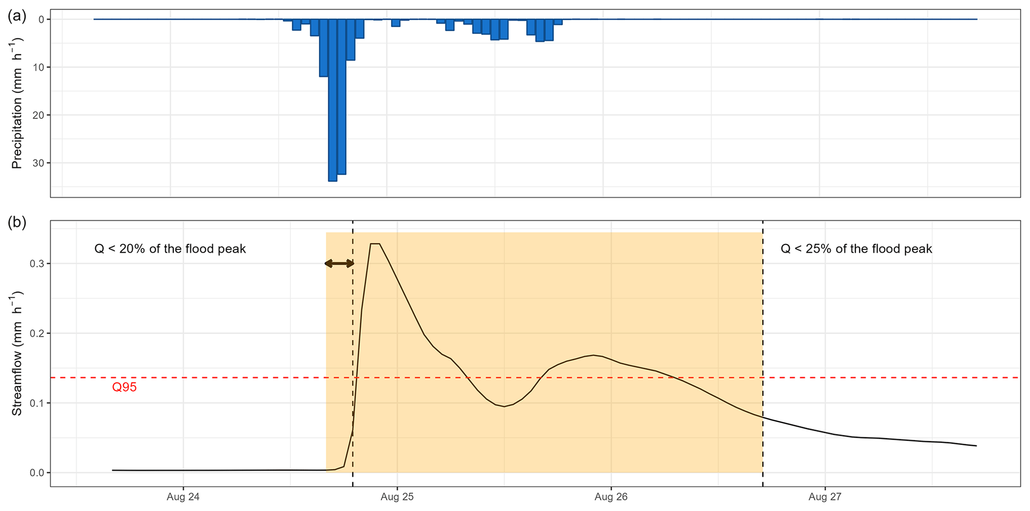
Figure A1 Flood event from 24 to 26 August 2009 on the Dore River at Saint-Gervais-sous-Meymont (K287191001). The yellow time window corresponds to the automatically selected event. The dashed red line represents the detection threshold set to the 95 % quantile. The dashed black lines refer to the initial entry and end dates of the events (respectively below 20 % and 25 % of the flood peak). The arrow here shows an extension of the event start due to the rapid rise in water level.

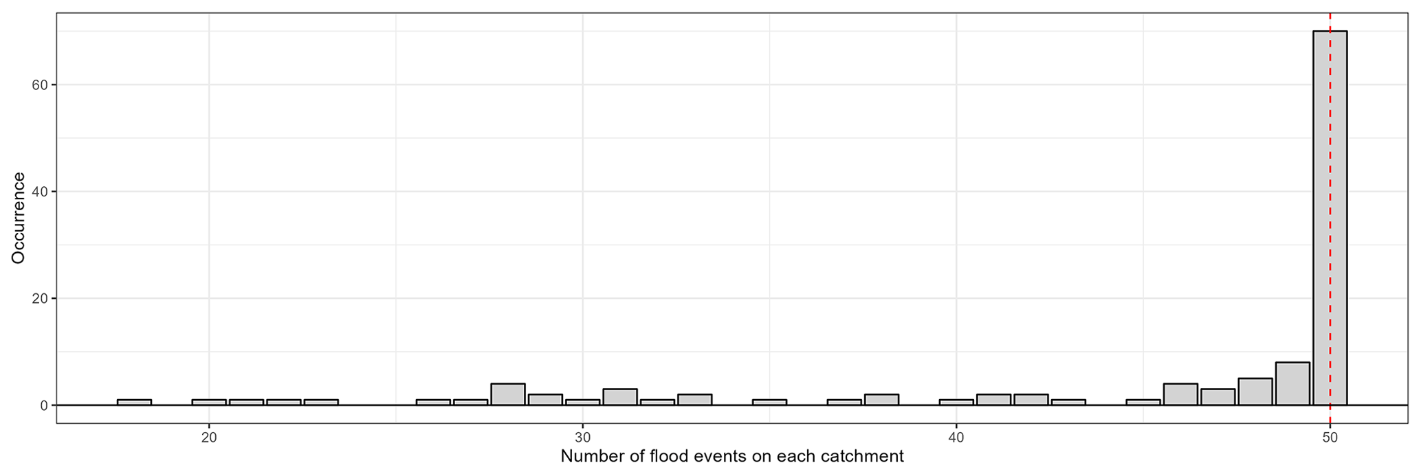
Figure A2 Distribution of the number of flood events in each catchment over the whole catchment set. The red line shows the maximum number allowed.

Appendix B: Event selection methodology: low-flow events

The selection procedure of low-flow events was based on the methodology developed and used by Caillouet et al. (2017). It is an automated procedure selecting periods under a threshold (fixed here to the 10 % quantile) and aggregating the intervals corresponding to the same event thanks to the severity index (Fig. B1).

Each selected event was visually inspected to mitigate the errors associated with automatic selection. This step is rather difficult because the quality of the low-flow data is quite heterogeneous (e.g. influenced by noise) from one catchment to another. In the end, 1332 events were selected. Figure B2 shows the distribution of the number of low-flow events in each catchment.

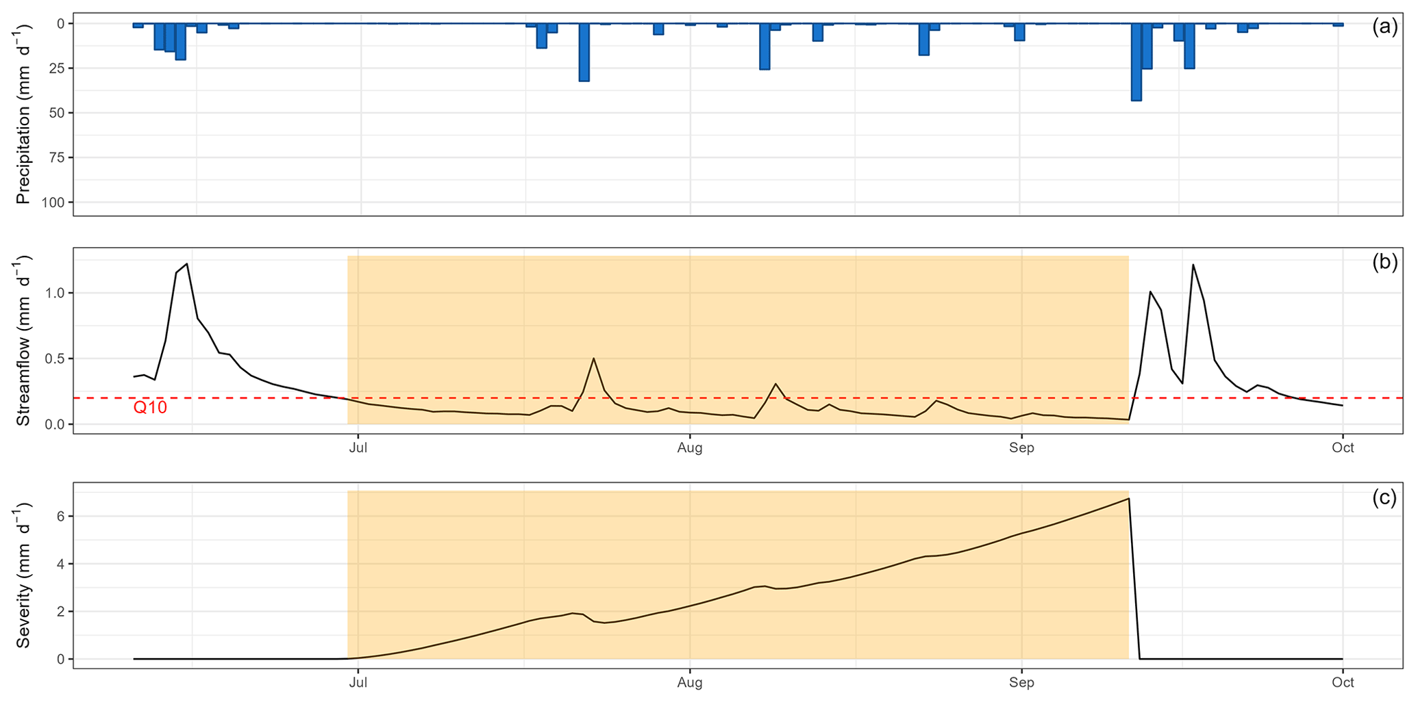
Figure B1 Low-flow event from summer 2015 on the Dore River at Saint-Gervais-sous-Meymont (K287191001). The yellow time window corresponds to the automatically selected event. The dashed red line represents the detection threshold set to the 10 % quantile for streamflow. The severity corresponds to the cumulated deficit under the threshold.

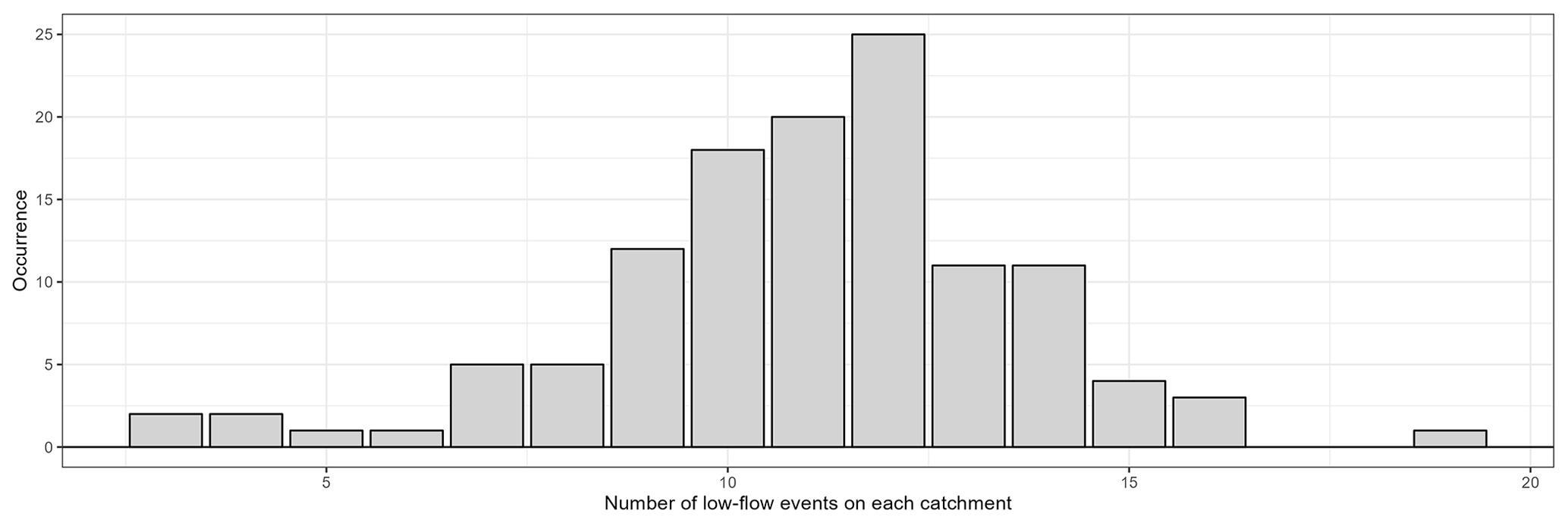
Figure B2 Distribution of the number of low-flow events in each catchment over the whole catchment set.

Appendix C: Uncertainty in KGE scores

Since efficiency criteria values depend on the variety of errors found in the evaluation period (see, for example, Berthet et al., 2010), this may impact the significance of performance differences between models and ultimately their comparison. Therefore, we tried to quantify the sampling uncertainty in KGE scores. The bootstrap–jackknife methodology proposed by Clark et al. (2021) was applied over our set of 121 catchments for the 39 lumped models (Fig. C1). The results show that for 90 % of the cases, the KGEs have uncertainties lower than 0.06 with a median of 0.02. However, differences can be noted according to the catchments; the structures; the calibration period; the period used to apply the bootstrap–jackknife; and, especially, the transformations used during the model calibration. Indeed, KGE values from simulations optimized for low flows are more uncertain than those optimized for medium or high flows.

Figure C2 compares the KGE uncertainty between the benchmark (all catchments are modelled with GR5H calibrated with the KGE calculated on Q^+0.1 in a lumped spatial framework) and the mixed multi-model approach (a combination of model with a variable spatial framework is chosen for each catchment). It shows that the MMM approach reduces uncertainty about the value of the performance score. We therefore consider an improvement to be significant as soon as a gain greater than 0.02 is achieved.

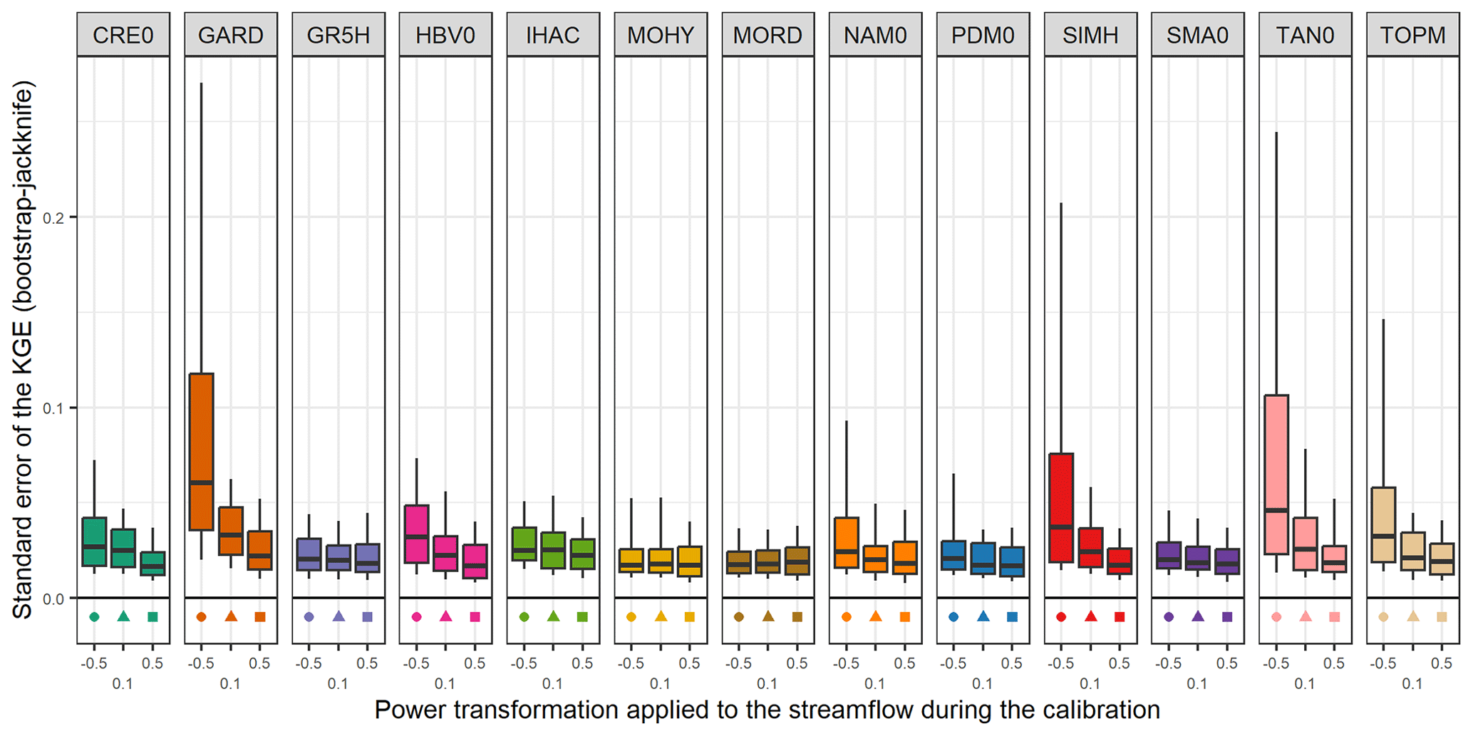
Figure C1 Distribution of standard error of the KGE obtained with the bootstrap–jackknife methodology over the 121 catchments. The box plots represent the 10 %, 25 %, 50 %, 75 %, and 90 % quantiles.

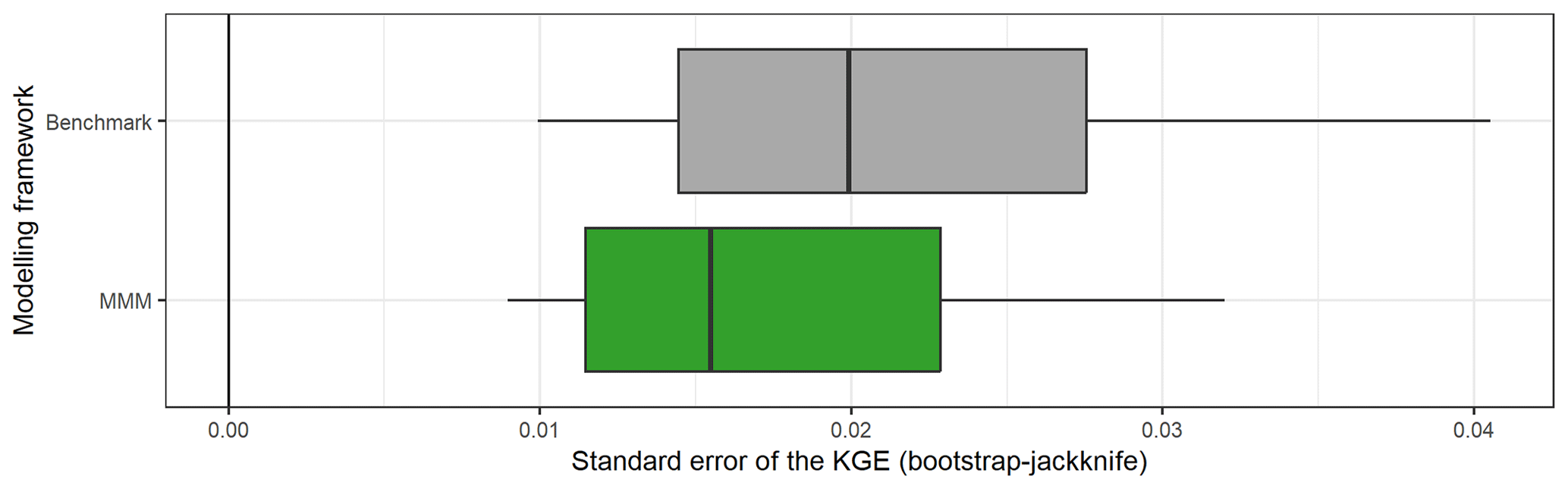
Figure C2 Comparison of the standard error of the KGE obtained with the bootstrap–jackknife methodology over the 121 catchments for the benchmark (one-size-fits-all model) and the mixed multi-model (MMM) approach. The box plots represent the 10 %, 25 %, 50 %, 75 %, and 90 % quantiles.