Technical note: A model of chemical transport in a wellbore–aquifer system

Wellbore is proven to be the only effective way of delivering chemicals to a target aquifer during a tracer test or aquifer remediation. The volume of original water in the operational well is a critical parameter affecting the concentration of injected tracers or chemicals in the wellbore in the early stages. We found that the calculation of the wellbore water volume by previous numerical methods was correct when the wellbore penetrates an unconfined aquifer but incorrect when the wellbore penetrates a confined aquifer, further resulting in errors in describing the solute transport of injected chemicals in confined aquifers, such as MODFLOW/MT3DMS or FEFFLOW. Such errors caused by MODFLOW/MT3DMS and FEFFLOW increased with increasing wellbore water volume. This was because the groundwater in both the wellbore and aquifer was assumed to be confined where the water level was higher than the aquifer's top elevation and the groundwater thickness was assumed to be equal to the aquifer thickness. Actually, when the wellbore penetrated a confined aquifer, the groundwater was only confined in the aquifer, while it was unconfined in the wellbore. In this study, the solute transport model is revised based on the mass balance in a well–aquifer system, with special attention given to the wellbore water volume. The accuracy of the new model was tested against benchmark analytical solutions. The revised model could increase the accuracy of reactive transport modeling in aquifer remediation through the wellbore.

1 Introduction

Wellbore is an effective way of delivering chemicals to a target aquifer for the purpose of parameter estimation in a tracer test or aquifer remediation (Anderson et al., 2015; El-Kadi, 1988). As groundwater flow is complex in the subsurface, the amount of chemicals to be delivered and the area of the final concentration after entering the aquifers have to be evaluated by mathematical models. Therefore, the robustness of the mathematical models of solute transport is critical for accuracy and interpretation. According to the treatment of solute transport in a wellbore, the mathematical models could be classified into two types, which will be reviewed in Sect. 2. The first type of mathematical model considers the wellbore to be an inner boundary condition of reactive transport in the aquifer (named the IBC model), and it is preferred by the analytical solutions, while in the second type of mathematical model, the well is treated as a source or sink (named the SS model), and they are preferred by the numerical solutions due to the complexity of hydrogeological conditions (like the heterogeneity and transiency of the flow field).

The SS models of the tracer test are composed of two parts: solute transport in the wellbore and the aquifer. In the confined aquifer, the wellbore is open to the air, hence making it unconfined. After a careful literature review, we found that previous numerical solutions of two-dimensional (2D) and three-dimensional (3D) SS models of the tracer test in the Cartesian coordinate system did not properly deal with the mixing processes between the original water and tracers entering the operational wellbore in a confined aquifer. The objectives of this study include the revisit of the treatment of wellbore storage in mathematical models of reactive transport in a wellbore–aquifer system, the revision of the numerical solution of the SS model describing the mixing processes between solutes in the wellbore during the solute transport, and the validation of the revised model.

2 Review of mathematical models of solute transport in a wellbore–aquifer system

2.1 The IBC model of solute transport

When the wellbore is considered an inner boundary condition, the wellbore–aquifer system reduces the aquifer system, as the concentration variation of the solute in the wellbore is not included in the governing equation (Veling, 2012; Wang and Zhan, 2013), e.g.,

$$\begin{array}{}\text{(1)}& \begin{array}{rl}{\displaystyle \frac{\partial \left(\mathit{\theta }{C}^k\right)}{\partial t}}& =L_{\mathrm{DSP}}\left(C^k\right)+L_{\mathrm{ADV}}\left(C^k\right)+L_{\mathrm{SSM}}\left(C^k\right)\\ & +L_{\mathrm{RCT}}\left(\mathit{\theta }{C}^k\right),t>\mathrm{0},\end{array}\end{array}$$

$$\begin{array}{}\text{(2a)}& {\displaystyle }{\left.C^k\left(r,z,t\right)\right|}_{r=r_{\mathrm{w}}}=f\left(z,t\right),t>\mathrm{0},\text{(2b)}& {\displaystyle }\begin{array}{rl}& {\left.\mathrm{or}\left[v_{\mathrm{r}}{C}^k\left(r,z,t\right)-{\mathit{\alpha }}_{\mathrm{r}}\left|v_{\mathrm{r}}\right|{\displaystyle \frac{\partial C^k\left(r,z,t\right)}{\partial r}}\right]\right|}_{r=r_{\mathrm{w}}}\\ & =v_{\mathrm{r}}f\left(z,t\right),t>\mathrm{0},\end{array}\end{array}$$

where C^k is the dissolved concentration of species k (ML⁻³); k is a positive integral to account for the number of species (dimensionless); t is time (T); r is the radial distance from the wellbore (L); z is the vertical distance; θ is the porosity of the porous medium (dimensionless); r_w is the wellbore radius (L); α_r and v_r are the radial dispersivity (L²T⁻¹) and radial flow velocity (LT⁻¹) respectively; L_DSP(⋅), L_ADV(⋅), L_SSM(⋅), and L_RCT(⋅) are the operators for the dispersion, advection, and other sinks and sources excluding the discharge and recharge in the wellbore and chemical reaction terms, respectively; and f(t) represents the concentration variations of the solute in the wellbore, which is a function of time. Equation (1) is the multi-species governing equation of reactive transport. Equations (2a)–(2b) are the inner boundary conditions representing the resident concentration continuity and the flux concentration continuity at the well–aquifer interface, respectively, while Eq. (2b) is recommended since it could keep the mass balance for solute transport in the aquifer. The difference between them can be seen in Schwartz et al. (1999) and Novakowski (1992).

This type of model is generally established in the radial coordinate system, such as Wang and Zhan (2013). This is because the flow field is radial when only one well exists and the regional flow (or ambient flow) is negligibly small. The advantage of the radial coordinate system is that it could simplify the mathematical models from two dimensions into one dimension (Chen, 1985; Chen et al., 2012; Novakowski, 1992) or from three dimensions into two dimensions (Huang et al., 2010; Chen, 2010; Chen et al., 2011), for which elegant analytical models may be developed. As for the 2D radial transport, the operators of L_DSP(⋅), L_ADV(⋅), L_SSM(⋅), and L_RCT(⋅) are

$$\begin{array}{}\text{(3)}& {\displaystyle }\begin{array}{rl}{L}_{\mathrm{DSP}}\left(C^k\right)& ={\displaystyle \frac{\mathrm{1}}{r}}{\displaystyle \frac{\partial }{\partial r}}\left(r{D}_{rr}{\displaystyle \frac{\partial C^k}{\partial r}}+r{D}_{rz}{\displaystyle \frac{\partial C^k}{\partial z}}\right)\\ & +{\displaystyle \frac{\partial }{\partial z}}\left(D_{zr}{\displaystyle \frac{\partial C^k}{\partial z}}+D_{zz}{\displaystyle \frac{\partial C^k}{\partial z}}\right),\end{array}\text{(4)}& {\displaystyle }{L}_{\mathrm{ADV}}\left(C^k\right)=v_{\mathrm{r}}{\displaystyle \frac{\partial C^k}{\partial r}}+v_z{\displaystyle \frac{\partial C^k}{\partial z}},\text{(5)}& {\displaystyle }{L}_{\mathrm{SSM}}\left(C^k\right)=q_{\mathrm{s}}{C}^k,\text{(6)}& {\displaystyle }{L}_{\mathrm{RCT}}\left(\mathit{\theta }{C}^k\right)=\sum R_n,\end{array}$$

where D_rr, D_rz, D_zr, and D_zz are the four components of the dispersion coefficient tensor (L²T⁻¹), respectively; ∑R_n is the chemical reaction term (ML⁻³T⁻¹); q_s is the volumetric flow rate per unit volume which does not include the pumpage of the wellbore (T⁻¹); and v_z is the vertical flow (LT⁻¹).

However, these types of models have two shortcomings. Firstly, the flow field may not be radial in realistic aquifer settings, for instance, when more than one well exists or the regional flow can be ignored. Secondly, Eq. (2a) or Eq. (2b) is used to describe the transport at the well screen, and the concentration in the wellbore is required, e.g., f(z,t), which may be unknown in reality. For simplicity, many studies have assumed that f(z,t) equals the concentration of the injected solute inside the wellbore (Chen, 1985, 2010; Phanikumar and McGuire, 2010; Yeh and Chang, 2013):

$$\begin{array}{}\text{(7)}& f\left(z,t\right)=C_{\mathrm{inj}}^k,\end{array}$$

where $C_{\mathrm{inj}}^k$ is the concentration of species k in the injected solute (ML⁻³). This is not true, since Eq. (7) does not consider the mixing processes between the original water and tracers entering the operational wellbore, and it overestimates the values of the concentration in the wellbore. Novakowski (1992) presented a well model considering the wellbore storage for different scenarios based on the mass balance principle, while the flow field was assumed to be in steady state and the mixing processes were assumed to be instantaneously completed.

2.2 The SS model of solute transport

Because of the limitations of the IBC model, the popular way is to consider the wellbore as a source or sink term in the governing equation of reactive transport in the numerical modeling. The governing equation of multi-species reactive transport in the wellbore–aquifer system becomes (Konikow and Grove, 1977; Zheng and Wang, 1999)

$$\begin{array}{}\text{(8)}& \begin{array}{rl}{\displaystyle \frac{\partial \left(\mathit{\theta }{C}^k\right)}{\partial t}}& =L_{\mathrm{DSP}}\left(C^k\right)+L_{\mathrm{ADV}}\left(C^k\right)+L_{\mathrm{SSM}}\left(C^k\right)\\ & +L_{\mathrm{RCT}}\left(\mathit{\theta }{C}^k\right)+q_{\mathrm{w}}{C}_{\mathrm{w}}^k,t>\mathrm{0},\end{array}\end{array}$$

where q_w is the volumetric flow rate per unit volume of the aquifer (T⁻¹), and it is positive for injection (when the well acts as a source) and negative for extraction (when the well acts as a sink); $C_{\mathrm{w}}^k$ is the concentration of species k (ML⁻³), and it is equal to C^k in the case of extraction (q_s<0); the operators of L_DSP(⋅) and L_ADV(⋅) are different from the ones defined in Eq. (1), for instance,

$$\begin{array}{}\text{(9)}& {\displaystyle }{L}_{\mathrm{DSP}}\left(C^k\right)={\displaystyle \frac{\partial }{\partial x_i}}\left(\mathit{\theta }{D}_{ij}{\displaystyle \frac{\partial C^k}{\partial x_j}}\right),\text{(10)}& {\displaystyle }{L}_{\mathrm{ADV}}\left(C^k\right)={\displaystyle \frac{\partial }{\partial x_i}}\left(\mathit{\theta }{v}_i{C}^k\right),\end{array}$$

where x_i is the distance (L) along the respective Cartesian coordinate axis, i= 1, 2, and 3, representing the x, y, and z axes, respectively; D_ij is the hydrodynamic dispersion coefficient tensor (L²T⁻¹); and v_i is the flow velocity. The definitions of L_SSM(⋅) and L_RCT(⋅) are the same as the ones in Eq. (1). The boundary of Eq. (4) is set far away from the well, where the concentration is equal to the background value.

Different from the first approach in Sect. 2.1, only the values of q_w and $C_{\mathrm{w}}^k$ are required, which are generally available. Equations (8)–(10) have been widely employed for solute transport modeling in many software packages, like MODFLOW/MT3DMS (Zheng and Wang, 1999), FEFLOW (Trefry and Muffels, 2007), or TOUGH2 (Pruess et al., 1999).

2.3 Groundwater flow model of the tracer test in the confined aquifer

Solute transport in aquifers is mainly controlled by groundwater flow, like dispersion, advection, and reactions, and therefore the mathematical models of groundwater flow have to be solved to obtain the flow velocity or the hydraulic head before solving the models of solute transport. For instance, in the software package MODFLOW/MT3DMS, the modeling of groundwater flow by MODFLOW is run first to produce the spatiotemporal flow field for modeling solute transport by MT3DMS.

3 Errors of the previous numerical models

The MODFLOW/MT3DMS package and the FEFLOW package are based on the finite-difference method and the finite-element method, respectively. As MODFLOW/MT3DMS is free and open source, it can be easily revised, and we mainly analyze the errors of this numerical model. The finite-difference scheme of the MODFLOW/MT3DMS model of the tracer test in confined aquifers in the wellbore–aquifer system is (Konikow and Grove, 1977; Zheng and Wang, 1999)

$$\begin{array}{}\text{(11)}& \begin{array}{rl}{\mathrm{MA}}_{\mathrm{Cell}}& ={\mathrm{NMF}}_x+{\mathrm{NMF}}_y+{\mathrm{NMF}}_z+{\mathrm{NMFSS}}_{\mathrm{Cell}}\\ & +{\mathrm{NMFR}}_{\mathrm{Cell}},\end{array}\end{array}$$

where

$$\begin{array}{}\text{(12a)}& {\displaystyle }{\mathrm{NMF}}_x=-{\displaystyle \frac{\partial }{\partial x}}\left(C^k\mathit{\theta }{v}_x^{*}\mathrm{\Delta }y\mathrm{\Delta }z\right)\mathrm{\Delta }x,\text{(12b)}& {\displaystyle }{\mathrm{NMF}}_y=-{\displaystyle \frac{\partial }{\partial y}}\left(C^k\mathit{\theta }{v}_y^{*}\mathrm{\Delta }x\mathrm{\Delta }z\right)\mathrm{\Delta }y,\text{(12c)}& {\displaystyle }{\mathrm{NMF}}_z=-{\displaystyle \frac{\partial }{\partial z}}\left(C^k\mathit{\theta }{v}_z^{*}\mathrm{\Delta }x\mathrm{\Delta }y\right)\mathrm{\Delta }z,\text{(12d)}& {\displaystyle }{\mathrm{NMFSS}}_{\mathrm{Cell}}=W_{\mathrm{s}}{C}_{\mathrm{s}}^k\mathrm{\Delta }x\mathrm{\Delta }y\mathrm{\Delta }z,\text{(12e)}& {\displaystyle }{\mathrm{NMFR}}_{\mathrm{Cell}}=\mathit{\theta }\mathrm{\Delta }x\mathrm{\Delta }y\mathrm{\Delta }z\sum R_k,\text{(12f)}& {\displaystyle }{\mathrm{MA}}_{\mathrm{Cell}}={\displaystyle \frac{\partial }{\partial t}}\left(C^k\mathit{\theta }\mathrm{\Delta }x\mathrm{\Delta }y\mathrm{\Delta }z\right),\end{array}$$

where $v_x^{*}$, $v_y^{*}$, and $v_z^{*}$ are instantaneous mass velocities (LT⁻¹) along the x, y, and z axes, respectively; W_s is the volumetric flux per volume of porous medium (T⁻¹); $C_{\mathrm{s}}^k$ is the concentration (ML⁻³) of the solute in the source or sink fluid; Δx, Δy, and Δz are the dimensions (L) of the cell along the x, y, and z axes, respectively; MA is the mass accumulation rate (MT⁻¹); NMF is the net mass flux (MT⁻¹); NMFSS is the net mass flux by source and sink (MT⁻¹); and NMFR is the net mass flux by reactions (MT⁻¹). When Δx=Δy and $\mathrm{\Delta }x\mathrm{\Delta }y=\mathit{\pi }{r}_{\mathrm{w}}^{\mathrm{2}}$ in the wellbore cell, W_s is the injection or extraction rate per volume, and $C_{\mathrm{s}}^k$ is the concentration of the injected or extracted solute.

Equations (11)–(12) are used in the WELL package of MT3DMS for modeling reactive transport in the wellbore–aquifer system, which is suitable for the one-cell wellbore model, not for the multi-node well (MNW) model. The MNW model refers to a case when the wellbore is vertically discretized into several cells (e.g., Cell 1, Cell 2, Cell 3, and Cell 4, as shown in Fig. 1). In the one-cell wellbore model, the intra-borehole flow is ignored. As for the MNW model, the intra-borehole flow is considered, and there is a special package developed for both groundwater flow and solute transport based on MODFLOW/MT3DMS, named the MNW package (Konikow and Hornberger, 2006; Konikow et al., 2009).

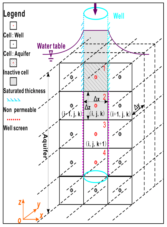
Figure 1 Schematic diagram of the grid system in a numerical simulation of a partially penetrating well. Black lines represent the discretization of the aquifer, including the wellbore in the aquifer (e.g., Cell 1, Cell 2, Cell 3, or Cell 4). The part of the wellbore located above the aquifer is not included in the grid system.

Equations (12a)–(12f) demonstrate that the weaknesses of the second type of model are that the wellbore is treated as a part of the aquifer, resulting in the following two problems. Firstly, the porosity of the wellbore is unity, but it is assumed to be the same as the porosity of the surrounding aquifer. Secondly, the term θΔxΔyΔz represents the volume of water in the cells of the grid system in Fig. 1, regardless of the aquifer and wellbore; it remains constant. Actually, the aquifer cells are different from the wellbore cells in bearing groundwater. In the confined aquifer cells, the volume of water is not affected by the variation in the hydraulic head; however, in the wellbore, the volume of water directly changes with the variation in the water level.

To test the effect of assumptions included in MODFLOW/MT3DMS and FEFFLOW on solute transport in a wellbore–aquifer system, we employ a proven analytical solution that will serve as the benchmark of comparison. Unfortunately, it seems not to be easy to derive a general-purpose analytical solution that can accommodate many realistic field conditions, such as flow transiency. It is also necessary to test the new model with the analytical solution considering the actual well construction, such as the skin effect. However, the available analytical solutions to the two-region model have not considered wellbore storage. For instance, Chen et al. (2012) assumed that f(z,t) in Eq. (2a) was constant and independent of location and time and was equal to the concentration of the injected solute. Therefore, we will employ the analytical solution of an injection test by Novakowski (1992), who considered wellbore storage.

Figure 2a and 2b show the comparison of the breakthrough curves (BTCs) with the analytical and numerical methods in the wellbore, where the vertical axis represents the relative (or normalized) concentration $C/C_{\mathrm{0}}$ and C₀ is the constant concentration of the injected solute. The legend of “ANA” represents the analytical solutions by Novakowski (1992). The parameters used in this case are as follows. The aquifer dimensions are 100 m$\times \mathrm{100}\mathrm{m}\times \mathrm{6}\mathrm{m}$; the horizontal hydraulic conductivity is 10 m d⁻¹; the horizontal anisotropy is 1.0, where the horizontal anisotropy is the ratio between the two horizontal principal components of the hydraulic conductivity; the injection flow rate is 20 m³ d⁻¹; the porosity is 0.3; the longitudinal dispersivity is 0.5 m; the ratio of the horizontal transverse dispersivity to the longitudinal dispersivity is 0.1; the ratio of the vertical transverse dispersivity to the longitudinal dispersivity is 0.01. As the well radius is always constant, three sets of initial conditions of the hydraulic head are employed to test the influence of the water level on the wellbore storage: h₀= 6 m, h₀= 30 m, and h₀= 60 m. A greater initial head implies a greater water level in the wellbore. Since the depth of the wellbore might be greater than 100 m and sometimes 1000 m for a deep confined aquifer, the maximum value of 60 m for h₀ is not unusual for the initial hydraulic head. As the flow is assumed to be in a steady state, the information of the specific yield and the specific storage is not needed. The spatial discretizations are Δx=0.4 m, Δy=0.4 m, and Δz= 6 m. The aquifer is vertically discretized into one layer. This is because the flow direction is radially horizontal for a well fully penetrating a homogeneous aquifer. The steady-state drawdown in the wellbore is set to −0.346 m for all the cases.

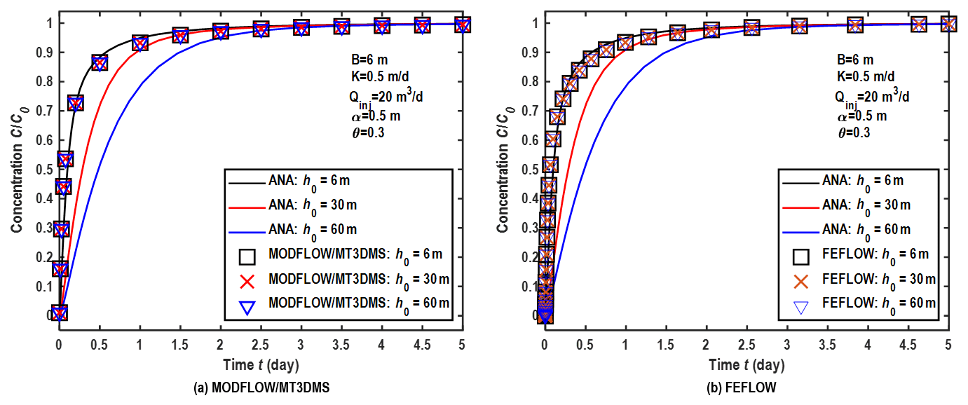
Figure 2 Comparison between BTCs based on analytical and numerical methods in the wellbore under steady-state flow conditions. ANA: analytical solutions.

A point to note is that the wellbore is a cylinder in the analytical solution, while it is approximated as a cuboid in the numerical solution by MODFLOW/MT3DMS. To ensure the same water volume used in both the analytical and numerical solutions, the well radius (r_w) of the analytical solution is calculated by the following equation:

$$\begin{array}{}\text{(13)}& r_{\mathrm{w}}=\sqrt{{\displaystyle \frac{\mathrm{\Delta }x\mathrm{\Delta }y}{\mathit{\pi }}}}.\end{array}$$

Figure 2a and 2b show that the numerical solution by the previous MODFLOW/MT3DMS code and FEFLOW is independent of the water level in the wellbore, which is close to the analytical solution when the initial water level inside the wellbore is 6 m (the same as the aquifer thickness). However, when the initial water level inside the wellbore is substantially different from the aquifer thickness of 6 m, considerable discrepancies can be seen between the analytical and numerical solutions. These two figures demonstrate that the previous models of Eqs. (8)–(12) may cause significant errors in describing solute transport around a wellbore when the initial water level inside the wellbore is considerably different from the aquifer thickness.

4 Revised finite-difference scheme of the SS models

In this study, Eqs. (8)–(12) are called the “previous models” hereinafter and will be revised by considering the water level variation in a wellbore. Including the wellbore cells in the numerical simulation of flow in a well–aquifer system poses new challenges. For instance, the simulated aquifer is confined, whereas the simulated open wellbore is unconfined. The wellbore may include permeable screen sections and impermeable casings, as shown in Fig. 1. Therefore, how to treat the wellbore cells in the numerical models needs to be clarified.

Figure 1 shows the grid system for the general case in the numerical simulation. The well is discretized into several cells, e.g., Cell 1, Cell 2, Cell 3, and Cell 4, and such a well is named a multi-node well. When the well is discretized into one cell, a multi-node well reduces to a one-cell well. Cell 2, Cell 3, and Cell 4 in Fig. 1 represent the permeable screen, which could be treated as point sources or sinks in the model. Cell 1 in Fig. 1 represents the impermeable casing, which is the uppermost cell above the screen inside the wellbore.

As for Cell 1, the lateral boundary is impermeable, which implies that it can only exchange water with Cell 2. Therefore, Cell 1, the wellbore above Cell 1, and Cell 2 can be combined into one cell, e.g., a revised Cell 2. The volume of water in this revised Cell 2 is the summation of water in Cell 1, water in the wellbore above Cell 1, and water in the original Cell 2. That is, the volume of water in this revised cell is ΔxΔyB_Cell2,w, where $B_{\mathrm{Cell}\mathrm{2},\mathrm{w}}=h_{\mathrm{w}}-z_{\mathrm{Cell}\mathrm{2},\mathrm{bot}}$; z_Cell2,bot is the vertical coordinate of the bottom of Cell 2; h_w is the water level of the wellbore. For a confined aquifer, one has $B_{\mathrm{Cell}\mathrm{2},\mathrm{w}}>\mathrm{\Delta }{z}_{\mathrm{Cell}\mathrm{2},\mathrm{w}}$, where Δz_Cell2, w represents the vertical dimension of Cell 2. The validity of such a treatment will be investigated in Sect. 4.2.

Therefore, the mass balance for the revised Cell 2 should be

$$\begin{array}{}\text{(14)}& {\mathrm{MA}}_{\mathrm{Cell}\mathrm{2}}={\displaystyle \frac{\partial }{\partial t}}\left(C^k\mathrm{\Delta }x\mathrm{\Delta }y{B}_{\mathrm{Cell}\mathrm{2},\mathrm{w}}\right),\end{array}$$

and Eq. (12d) becomes

$$\begin{array}{}\text{(15)}& {\mathrm{NMFSS}}_{\mathrm{Cell}}=W_{\mathrm{s}}{C}_{\mathrm{s}}^k\mathrm{\Delta }x\mathrm{\Delta }y{B}_{\mathrm{Cell}\mathrm{2},\mathrm{w}}.\end{array}$$

Since the porosity of the revised Cell 2 is unity, NMFR_Cell in Eq. (11) becomes

$$\begin{array}{}\text{(16)}& {\mathrm{NMFR}}_{\mathrm{Cell}}=\mathrm{\Delta }x\mathrm{\Delta }y{B}_{\mathrm{Cell}\mathrm{2},\mathrm{w}}\sum R_k.\end{array}$$

The other terms of the revised Cell 2 in Eq. (11) are the same as their counterparts in Eq. (12a)–(12f). As for the other wellbore cells, the mass balance equations are the same as the ones in Eq. (11), except that porosity is set as unity. As for the aquifer cells, the mass balance equations are the same as Eq. (11).

Similar to MODFLOW/MT3DMS, the finite-difference method will be employed to solve Eq. (8). The code of MT3DMS will be revised to accommodate the above special treatments of the wellbore cells (particularly the revised Cell 2 in Fig. 2) in this study. The flow field is computed by MODFLOW. The changes in the original MT3DMS code are explained in Sects. S1 and S2 in the Supplement.

As for a one-cell wellbore (when the well is discretized into a cell), solute transport in the well could be similarly treated by the equations used in the revised Cell 2.

In actual applications, the flow field is complex for either an injection well or an extraction well, as shown in the laboratory-controlled experiment of Wang et al. (2018), due to turbulent flow caused by the injection–extraction apparatus (usually a pipe) with a smaller diameter than that of the wellbore itself. Different from transport in porous media, the mechanism of solute transport in the wellbore is similar to transport in surface water bodies (e.g., river). Therefore, the diffusion effect and advection are considered for solute transport in the wellbore, while mechanical dispersion is absent (because there are no porous media inside the wellbore). In this study, the MNW model (Konikow and Hornberger, 2006) is used to describe the groundwater flow and solute transport in the wellbore, which is based on MODFLOW/MT3DMS.

5 Accuracy of the revised finite-difference scheme of the SS models

Figure 3 shows the comparison of the BTCs by the analytical and revised numerical methods in the wellbore. The parameters used in this case are the same as the ones used in Fig. 2.

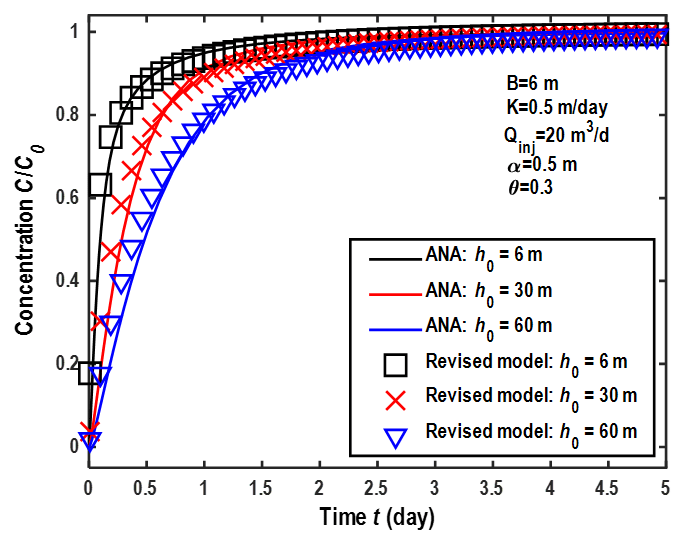
Figure 3 Comparison between the BTCs based on analytical and revised numerical methods in the wellbore under steady-state flow conditions. ANA: analytical solutions.

This figure shows the comparison between the analytical solution and the numerical solution by the revised MT3DMS code of this study, and they match well with each other, with some minor (but noticeable) discrepancies. Such minor discrepancies may be caused by two factors. First, the vertical surface area of the screen in the analytical solution (cylinder) is different from that in the numerical solution (cuboid) when the volume of the cuboid well is equal to the volume of the cylinder well. For instance, based on the setting of this study (r_w= 0.226 m, B= 6 m, Δx= 0.4 m), the surface area of a cylinder is 2πr_wB= 8.51 m², while the vertical surface area of a cuboid is 4ΔxB= 9.60 m². Such a difference in the surface area of the screen may generate a minor discrepancy between the analytical and numerical solutions. Second, numerical errors (like numerical dispersion) may not be completely eliminated in the finite-difference solution.

In addition, it is desirable to test the new models using an extraction well test. However, the analytical solution for such a case is not available if the wellbore storage must be taken into consideration. This is an open research problem that will be investigated in the near future.

6 Summary and conclusions

Solute transport in a well–aquifer system has attracted the attention of scholars in hydrogeology and environmental science during the past few decades. Due to the complexity of the flow field, numerical modeling has been widely used to study the fate and transport of contaminants in the subsurface through the interaction of an open borehole and the surrounding aquifer. By revisiting the previous mathematical model of reactive transport in the Cartesian coordinate system, we found that it could not properly describe the wellbore storage in the confined aquifer. In this study, a revised model is developed based on the mass balance principle in a well-confined aquifer system. The conclusions are summarized as follows. (1) In the early stage of the pumping phase, the volume of water in the wellbore is critical for the wellbore storage of solute transport. Greater volume results in a smaller concentration of solute in the wellbore, due to the mixing processes between the original water in the wellbore and water entering the wellbore or leaving the wellbore. (2) A revised model of reactive transport is proposed and tested against the analytical solutions, and it is much better than the previous models in describing the wellbore storage for a well penetrating a confined aquifer. (3) For the injection well test case, the previous models of reactive transport may cause errors, which are considerable in both the aquifer and the wellbore.