Disentangling coastal groundwater level dynamics in a global dataset

Groundwater level (GWL) dynamics result from a complex interplay between groundwater systems and the Earth system. This study aims to identify common hydrogeological patterns and to gain a deeper understanding of the underlying similarities and their link to physiographic, climatic, and anthropogenic controls of groundwater in coastal regions. The most striking aspects of GWL dynamics and their controls were identified through a combination of statistical metrics, calculated from about 8000 groundwater hydrographs, pattern recognition using clustering algorithms, classification using random forest, and SHapley Additive exPlanations (SHAPs). Hydrogeological similarity was defined by four clusters representing distinct patterns of GWL dynamics. These clusters can be observed globally across different continents and climate zones but simultaneously vary regionally and locally, suggesting a complicated interplay of controlling factors. The main controls differentiating GWL dynamics were identified, but we also provide evidence for the currently limited ability to explain GWL dynamics on large spatial scales, which we attribute mainly to uncertainties in the explanatory data. Finally, this study provides guidance for systematic and holistic groundwater monitoring and modeling and motivates a consideration of the different aspects of GWL dynamics, for example, when predicting climate-induced GWL changes, and the use of explainable machine learning techniques to deal with GWL complexity – especially when information on potential controls is limited or needs to be verified.

1 Introduction

When groundwater level (GWL) dynamics are tracked over time using groundwater hydrographs, the quantitative status of groundwater resources can be determined. Groundwater resources are exploited and measured locally, and GWL dynamics are subject to processes in their immediate local and regional environment (Bear, 2007), such as groundwater recharge rates, groundwater flow and pumping, and seawater intrusion (SWI) in coastal aquifers (Costall et al., 2020; Parisi et al., 2023). Hence, they are strongly location bound, and there is “a need for groundwater assessments at the field level” (United Nations, 2022). To this end, it is common practice in local studies to incorporate direct information from the groundwater system combined with expert knowledge of potential controls in numerical, statistical, or machine learning models (e.g., in Knowling et al., 2015; Güler et al., 2012; Lee et al., 2019). However, comprehensive knowledge of aquifer processes at the local scale is often lacking, posing even greater challenges for regional, continental, or global assessments of groundwater systems. Such larger scales are important, for example, with regard to large or transboundary aquifer systems, global virtual water trade, and international frameworks such as the UN Sustainable Development Goals (Donnelly et al., 2018; Nimmo et al., 2021). A systemic understanding of aquifer properties is the key to sustainable groundwater management and governance (Guppy et al., 2018; Elshall et al., 2020). Generalized scientific understanding of processes currently relies heavily on aggregating and upscaling local knowledge of groundwater's interactions with the Earth system; however, it is often lacking in direct observation-based evidence.

While it is largely unclear how GWL dynamics compare at large scales, the classification of GWL time series applied on such scales holds the potential to provide valuable insights into hydrogeological similarity (Barthel et al., 2021). For instance, these insights can prove to be valuable in assessing the coherence of large-scale process-based models by focusing on similarities in patterns and spatial trends rather than solely relying on the magnitude of aggregated errors, effectively mitigating the commensurability problem (Gleeson et al., 2021). In contrast, process understanding is limited when only the long-term mean or trend of GWL dynamics is considered (Lischeid et al., 2021; Gleeson et al., 2021; Baulon et al., 2022a).

The present study provides, for the first time, a classification of GWL dynamics at the global scale and is motivated by (a) a large number of GWL data that are available today – although not yet centralized and freely accessible for many regions of the world (United Nations, 2022) – and (b) the advancement of data-driven methods in Earth system sciences which are not only capable of finding patterns unseen by humans but also increasingly capable of explaining them (Reichstein et al., 2019; Shen et al., 2018). Previous studies have successfully applied inductive classification approaches (Olden et al., 2012), synthesizing different aspects of GWL dynamics at local to regional scales to investigate physiographic, climatic, and anthropogenic controls of GWL dynamics (Giese et al., 2020; Haaf et al., 2020; Ascott et al., 2020; Wunsch et al., 2021; Sorensen et al., 2021; Bosserelle et al., 2023); the function of groundwater in ecosystems (Martens et al., 2013); and runoff processes (Rinderer et al., 2019).

The primary focus of this study is to unveil GWL dynamics on global, regional, and local scales by analyzing local data that are distributed globally. The importance and vulnerability of coastal groundwater, which serves as a vital freshwater resource for ecosystems and large coastal communities with increasing water demands from groundwater (Oude Essink et al., 2010; Famiglietti, 2014; Ferguson and Gleeson, 2012; Moosdorf and Oehler, 2017), prompt this study to focus on disentangling GWL dynamics in coastal regions. We seek to answer the following research questions:

1. How is hydrogeological similarity observed on a global scale, and what are the implications of scaling for similarity patterns?

2. What are the key controlling factors for GWL dynamic patterns on a global scale, and how do they explain the variations observed at smaller scales?

3. What are the current opportunities for and barriers to deriving generalizations of dynamics–control relationships in groundwater using data-driven approaches?

The basis for answering these research questions is a newly compiled large and diverse dataset of about 8000 GWL time series of coastal aquifers from five continents. Information from the compiled and pre-processed time series (Sect. 2.1) was analyzed holistically using a set of previously defined statistical metrics from Heudorfer et al. (2019) that were computed from individual groundwater hydrographs (Sect. 2.2), thereby reducing their dimensionality (Wang et al., 2006). Section 3.1 derives GWL dynamic patterns in coastal regions by using unsupervised clustering techniques (Sect. 2.3) to group GWL time series based on information derived from the aforementioned statistical metrics. To deepen our understanding and elucidate key controlling factors for GWL dynamics, independent data encompassing various potential controls of GWL dynamics and associated surface processes were obtained from global map products (Sect. 2.4) and used to predict clusters in a random forest (RF) classification task (Sect. 2.5), with the results being presented in Sect. 3.2. The RF approach is a robust choice for classifying groundwater dynamics and is widely acknowledged in water science. With its capacity to capture non-linear dependencies and manage uncertainties such as unknown feature importance, overfitting, and outliers, RF provides a reliable tool for exploring complex interactions in natural processes (Tyralis et al., 2019). SHapley Additive exPlanation (SHAP) values were calculated for the RF model (Sect. 2.6). These are used to explain relationships between predicted clusters and descriptive features in Sect. 3.3. Such approaches of explainable machine learning are increasingly and successfully being applied in hydrology (Worland et al., 2019; Yang and Chui, 2021; Wunsch et al., 2022; Liu et al., 2022; Haaf et al., 2023). We discuss hydrogeological similarity results and the scaling effect (Sect. 4.1), evaluate derived explanations for GWL dynamic patterns (Sect. 4.2), and contextualize our findings within the framework of a case study region (Sect. 4.3). Section 5 provides concluding remarks.

2 Data and methods

The design of this study consists of the calculation of statistical metrics (hereafter referred to as indices) using compiled GWL time series and the clustering of GWL dynamics by applying unsupervised algorithms to the calculated indices. Subsequently, the clustering result that best differentiates characteristic groups of GWL dynamics was fed into an RF classifier together with local and regional natural and anthropogenic characteristics (hereafter referred to as attributes) from global map products that are potentially related to GWL dynamics. SHAP values were derived to understand the salient controls of each group of GWL dynamics. Unless stated otherwise, data pre-processing, modeling, and visualizations were done using Python (Python Software Foundation, 2021).

2.1 GWL time series and pre-processing

The GWL time series dataset analyzed in this study was compiled from the national and state governmental agencies listed in Table A1 in the Appendix. The data collection spanned from the years 2019 to 2022. Although attempts were made to find data for all coastal regions in the world, data collection focused on regions with a long coastline and large quantities of digitally available data. The wells from the compiled dataset are mainly located in northwestern Europe (Belgium, Denmark, France, Germany, Ireland, Netherlands, and Sweden) but also in Australia, South Africa, Brazil, Canada, and the United States. The wells are part of the GWL monitoring networks of the respective countries, but anthropogenic impact on GWL dynamics cannot be ruled out for all wells. In addition, wells may be affected by SWI and thus have variable density (Post et al., 2007). However, density gradients are not analyzed in this study because our focus is on absolute variations of the GWL. The GWL time series were selected based on the criteria outlined below.

1. There must be an availability of secondary information (in convertible units for homogenization), namely,

   • latitude and longitude of the well location (with variable accuracy),

   • reference vertical point or datum to measure the GWL depth,

   • date of observation.

2. Selection was based on well location and situation.

   • Selection of wells located within 100 km from the shoreline. This follows the definitions of Martínez et al. (2007) and Mangor et al. (2017), which focus on the ecological, economic, and social importance of coastal water resource planning. Thus, we did not aim to select aquifers directly related to marine processes, such as SWI.

   • Selection of shallow aquifers with mean GWLs less than 100 m below ground surface. It is important to note that this criterion is used as a directional guideline rather than an exact marker as there is uncertainty of up to a few meters in the absolute groundwater depth of observations referenced to sea level that were converted to ground surface reference with elevation data from the Shuttle Radar Topography Mission (SRTM) (Kulp and Strauss, 2018; Rodriguez et al., 2006; source-specific information in the Supplement).

3. Selection was based on temporal data availability criteria.

   • Data must be available for at least 4 complete calendar years within the years 1979 to 2019.

   • Time series must not have more than 10 % missing observations with data gap lengths of no larger than 2 weeks after aggregation to weekly time steps.

To obtain a homogeneous dataset, further source-specific pre-processing steps were necessary due to the very diverse data presentation, for example, regarding format, labels, and units. The reader is referred to the Supplement for notes on groundwater data collection and pre-processing. Potential anomalies or change points of the individual time series that indicate human activities, measurement, or reporting errors were removed using density-based spatial clustering of applications with noise (DBSCAN; Ester et al., 1996) combined – due to the large number of time series – with visual inspection of suspicious time series because we set the parameters rather conservatively; i.e., with the parameters set, DBSCAN detected outliers in more time series than we would have identified visually (Fig. A1). The systematic and additional visual inspection of groundwater time series was found to be beneficial, in line with recent publications (Barthel et al., 2022; Berendrecht et al., 2022; Lehr and Lischeid, 2020; Retike et al., 2022). Subsequently, temporal-availability criteria were checked once again, with remaining data gaps being linearly interpolated, and time series were transformed to the 0–1 scale for calculating indices.

2.2 Indices

We calculated a total of 45 indices for all GWL time series using an unpublished R package (R Core Team, 2021) that was developed with the study conducted by Heudorfer et al. (2019). These indices statistically aggregate and describe various aspects of groundwater hydrographs: their structure (e.g., interannual fluctuation heights and changes), distribution (e.g., alignment of the GWL with upper or lower fluctuation limits), and shape (e.g., steepness of hydrograph increases and decreases). For more detailed descriptions of the used indices (Table B1), we refer to Heudorfer et al. (2019). In addition, there are other promising signature-based time series characterizations for hydroclimatic time series, as selected and explored in Papacharalampous and Tyralis (2022), Papacharalampous et al. (2023), and Wunsch et al. (2021).

For our approach, the indices were computed from weekly aggregated time series with a length of at least 4 years (Sect. 2.1), which is at the lower end of the time period of 4 to 8 years recommended in Heudorfer et al. (2019). We decided to use short periods to enable a larger pool of time series to be taken into account for the global similarity analysis. The calculated set of indices transforms groundwater information into 45 static metrics. The resulting index value ranges were compared to those of Heudorfer et al. (2019) for quality controlling (Fig. B1). As a second outlier treatment (besides applying DBSCAN) of the original time series (see Sect. 2.1), time series with index values in the outermost 0.001 % of the index value distribution (4 × σ) were discarded.

2.3 Cluster analysis

Clustering of the indices was performed to find a generalized but robust representation of differing GWL dynamics in coastal regions. No specific indices were selected a priori to capture GWL dynamics holistically. This decision was made because indices differ in their ability to describe GWL dynamics depending on the flow system and the groundwater regime (Heudorfer et al., 2019; Giese et al., 2020; Haaf et al., 2020). For a similar reason, Papacharalampous et al. (2023) recommended using a large variety of time series characteristics for similarity analysis in hydrology.

A principal component analysis (PCA) was applied to index values after standardization to avoid redundancies among the 45 indices (Heudorfer et al., 2019; Fig. B2) and to reduce the number of features for clustering. The number of principal components (PCs) to be retained was set based on the scree plot and variance explained, yielding a dimensionality-reduced dataset, where indices are mapped as score values on the significant PCs. This was followed by a systematic search for the best aggregation of the scores using three different unsupervised clustering algorithms – agglomerative hierarchical clustering using the Ward criterion, k-means clustering, and Gaussian mixture. Unsupervised methods aim to learn more about the internal dependencies among the explanatory variables (Bergen et al., 2019), meaning that no expectations regarding the number or patterns of clusters were pre-set. Instead, evaluation metrics (Rousseeuw, 1987; Caliński and Harabasz, 1974; Davies and Bouldin, 1979) were used to find the best arrangement of data points into clusters via optimizing within-cluster and between-cluster similarity and dissimilarity.

Table 1 List (alphabetically by attribute category) of numeric (num) and categorical (cat) attributes used to relate GWL dynamics to controls and processes in this study.

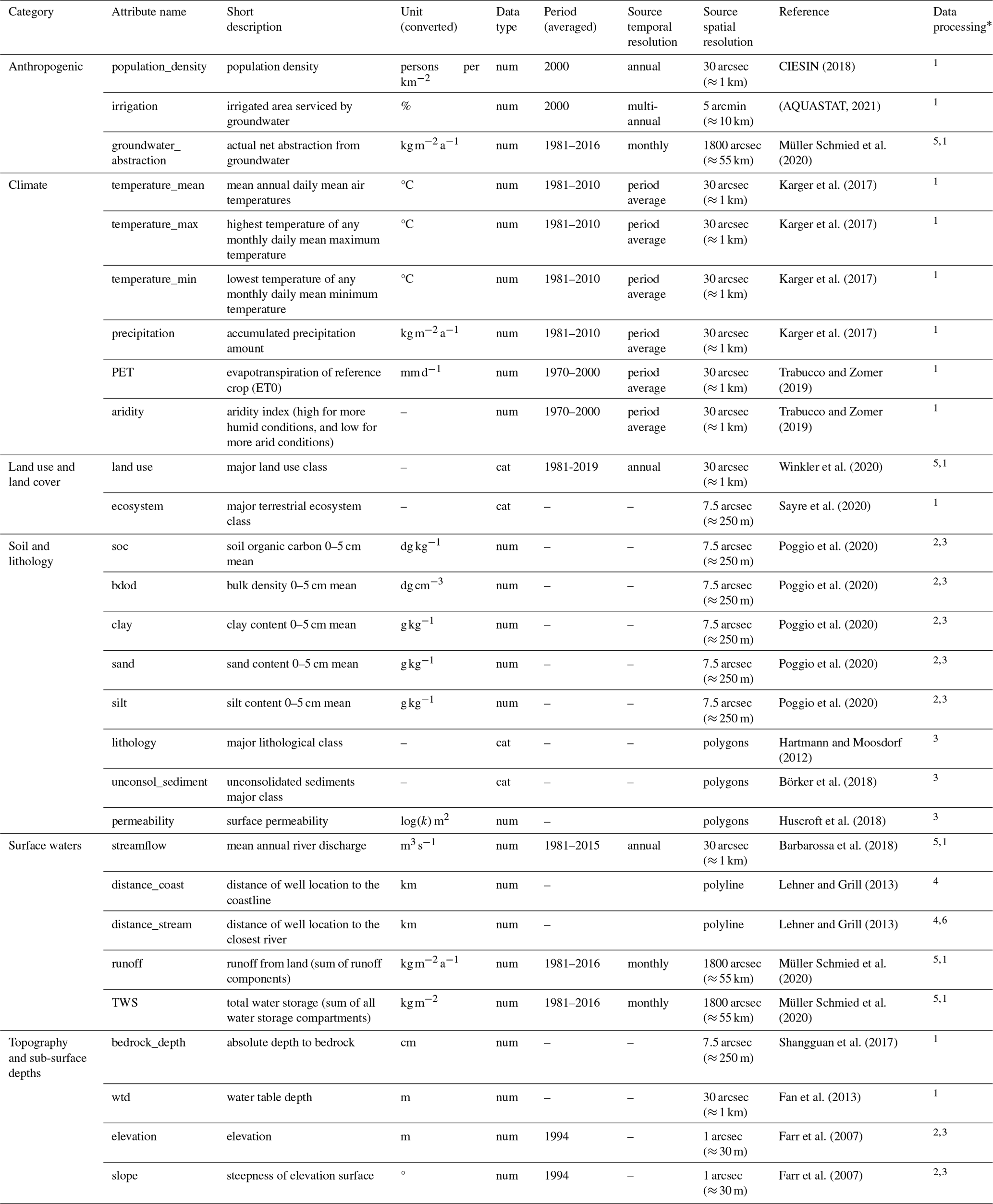
^* Individual data processing is explained in Sect. 2.4.

2.4 Attribute data

Understanding GWL dynamics requires integrated information from its manifold controls. These are typically represented by attribute data from hydrogeology, climate, land use and land cover, soil and lithology, surface waters, topography, and anthropogenic activity (Moeck et al., 2020; Rajaee et al., 2019; Díaz-Alcaide and Martínez-Santos, 2019). For river catchments, such datasets have already been collected for the regional scale (Addor et al., 2017; Klingler et al., 2021) and the global scale, most notably in the HydroATLAS (Linke et al., 2019). However, to date, there are no global datasets available that encompass the above-mentioned attributes specifically for groundwater studies (Haaf et al., 2020). Therefore, attributes mainly describing natural and anthropogenic characteristics and processes at the surface were collected from a variety of recent highest-resolution datasets available at the global scale (Table 1). These were used as proxies for global groundwater-specific datasets in this study.

While river catchments are typically well-defined by topography, subsurface catchments are often complex and vary on small scales (Vahdat-Aboueshagh et al., 2021). Despite recent efforts to develop a similar approach for calculating watersheds with a better representation for groundwater (Nölscher et al., 2022; Huggins et al., 2023), at the moment, there is no best-accepted method for groundwater-relevant delineation of various surface attributes on large scales. One approach to defining the contributing area of a groundwater well is to rely on the immediate vicinity and place a circular buffer around the monitoring site (Johnson and Belitz, 2009; Knoll et al., 2019). Using this approach, we extracted attributes as averages from buffers of 500 m radius placed around the well sites. The prepared attributes are of numerical and categorical type and contain information from multiple periods that have been unified where possible. The spatial resolution of the underlying source data is less than 30 arcsec, which is about 1000 m, except for hydrological data, which are derived from grids with a spatial resolution of only 1800 arcsec (approximately 55 km). Single- or multi-dimensional raster data and spatial vector data were downloaded and processed for the well locations as follows (applied to each dataset as indicated in the “Data processing” column in Table 1):

1. Average (median or majority) raster values were extracted for buffer geometries using the zonal statistics tool in ArcGIS Pro (Esri, 2022) with a cell size of 250 m.

2. Earth Engine Python API was accessed to directly calculate median raster values for buffer geometries and data download.

3. Average (median or majority) values from geospatial vector data were extracted for buffer geometries using the spatial join tool in ArcGIS Pro.

4. Distance was calculated between well points and polylines using the near tool in ArcGIS Pro.

5. Multidimensional rasters were aggregated to a single raster layer that presents the median or majority of superimposed raster cells of the period from 1981 to the latest available temporal dimension (make multidimensional raster tool and raster aggregation tool in ArcGIS Pro). Thereafter, we calculated the median of multiple raster files using the cell statistics tool in ArcGIS Pro.

6. For the distance of the well location to the closest river, we selected rivers that have a catchment area of at least 10 km² or an average river flow of at least 0.1 m³ sec⁻¹ or both.

2.5 Random forest model

The classification task was to assign the correct cluster out of n identified clusters (Sect. 2.3) using a set of attributes (Sect. 2.4). Well locations were considered for the RF classification (Breiman, 2001) only when data for all attributes were available. Furthermore, to avoid multiple clusters for a single combination of attributes, the cluster with the highest frequency was selected. The instance was retained if the identified cluster constituted more than 50 % of all clusters associated with that specific combination of attributes. The categorical attributes of land use, ecosystem, unconsolidated sediment, and lithology were pre-processed for their use in the RF model using one-hot encoding.

The RF model was optimized and evaluated with a stratified split of the dataset into a group for training and optimization (80 % of the data) and a group for testing (20 % of the data), taking into account an imbalanced dataset, where not all clusters have equal numbers of wells assigned and where regions are not represented equally by the dataset. For model optimization, hyperparameters were tuned within a 5-fold cross-validation framework. RF is a tree-based method that contains structures for feature selection (Breiman, 2001). No explicit feature selection was applied during pre-processing or model optimization, driven by the objective of exploring the relative importance and effects of all potential controls, as well as their collective impacts on GWL dynamics. Evaluation during model optimization and with the testing data of the optimized model was carried out using the model accuracy, calculated as the total number of correctly assigned classes divided by the sample number. In addition, the optimized model, i.e., the success of the classifier, was evaluated with metrics for the individual clusters: precision, recall, and F1 score. Here, precision is the number of correctly identified wells per cluster divided by all the times the model predicts that cluster. Recall is the number of correctly identified wells per cluster divided by the total number of wells in that cluster. The F1 score is 2 times the multiplication of precision and recall (2 × precision × recall) divided by the sum of precision and recall. RF, in general, works reasonably well when using the default values of hyperparameters in common algorithms (Probst et al., 2019). However, performance improvements can still be achieved by tuning, in particular, the number of trees that should be set high enough for robust results and the number of features considered for each time the tree is split. Up to 2000 trees were tested in combination with either all features or their square root being considered when looking for the best split using two different splitting criteria (Gini impurity and entropy: Breiman, 2001).

2.6 SHAP analysis

SHapley Additive exPlanation (SHAP) values (Lundberg et al., 2020) were used to investigate the feature attributions (feature importance and feature effects) to explain the RF classification. The three-dimensional space of SHAP values for the multiclass problem of this study is given by the number of clusters; the number of samples; and the number of features, i.e., attributes. Larger SHAP values for a specific cluster correspond to a higher probability of the cluster label. SHAP values of the samples that are part of the test dataset were analyzed collectively to explain how attributes impact the classification of the model. This corresponds to a global explanation of the model. For some analyses, SHAP values were combined for the attribute categories listed in Table 1. The SHAP values of individual instances, i.e., well sites, were combined with regional information to discuss the extent to which the generalized GWL dynamics derived through the index approach of this study can be explained in a case study region. When explaining controls of GWL dynamics from SHAP values, it is important to consider the interrelationships between the features. From the point of redundant features, the model is mainly trained on the feature with the most significant information in combination with other selected features. Hence, variables that combine information included in other features are generally ranked higher and reduce the ranking of the other redundant features.

3 Results

3.1 Identification of groundwater level dynamic patterns

Application of the time series selection criteria from Sect. 2.1 resulted in a set of 8574 GWL time series for which 45 indices were calculated. After removing time series with extreme index values (Sect. 2.2), a dataset with indices for 7888 time series remained. The value ranges for each of the different indices are comparable to those found by Heudorfer et al. (2019) (Fig. B1). Several indices showed a strong linear correlation (Fig. B2). From the PCA, five PCs represented 70 % of the variability of the linearly combined indices, while the first three PCs already described more than half of the variability (Fig. C1). The top five PCs served as input for the three clustering algorithms. These algorithms yielded similar results, where the highest cluster separation was achieved with three or four clusters (CL). The k-means clustering yielded the best cluster separation compared to hierarchical clustering and Gaussian mixture for all three evaluation criteria for cluster separation (Fig. C2). Comparing the cluster membership of wells, cluster composition based on k-means clustering is found to be quite similar to hierarchical clustering for most well sites (Fig. C3). The various characteristics of GWL dynamics can be assumed to exhibit complex and non-linear interlinkages in the multidimensional space.

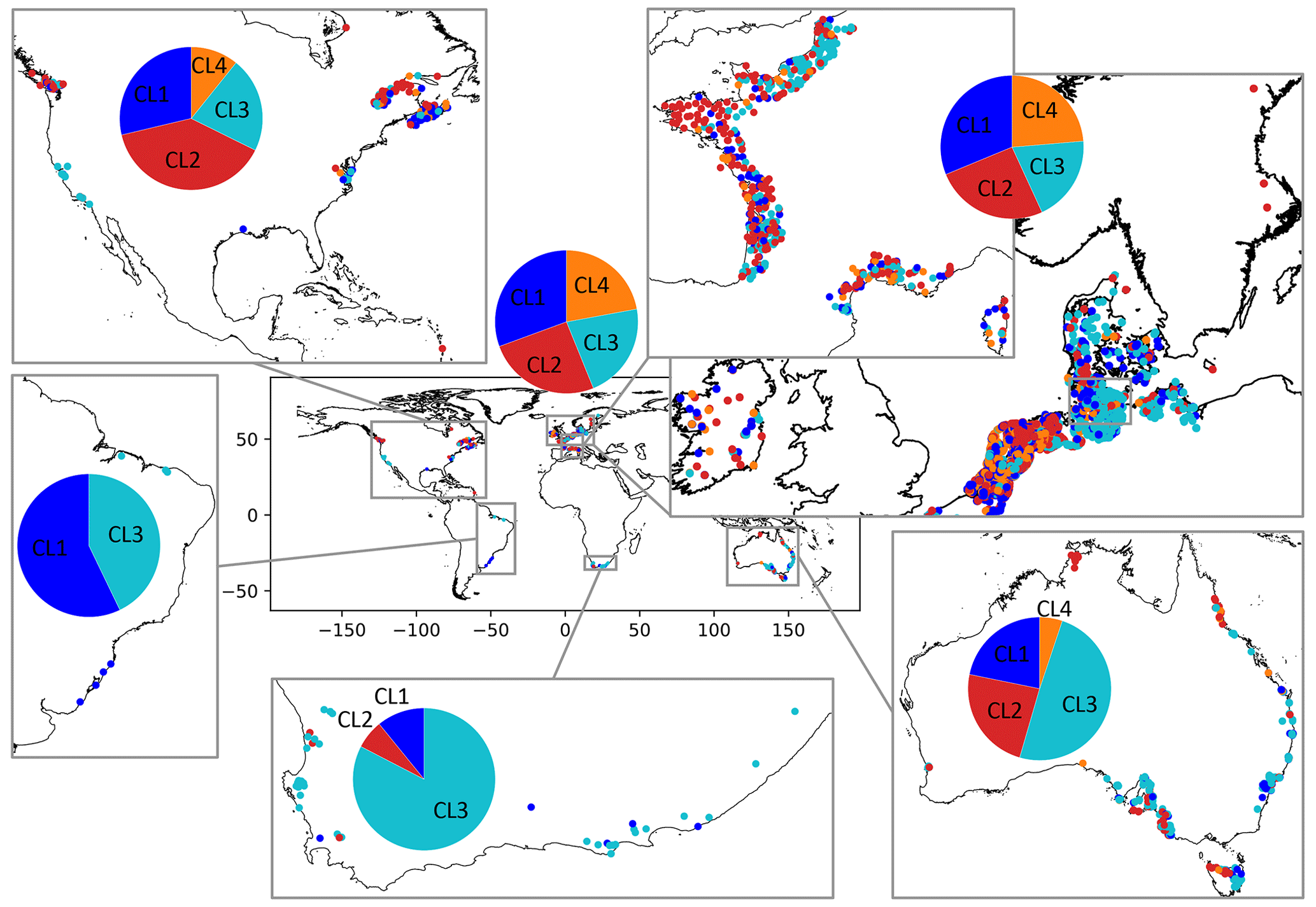
Figure 1 Assignment of clusters to well locations globally (center) and in coastal regions in North America, Europe (enlarged map of France and northwestern Europe), Australia, South Africa, and Brazil. Due to the large scale, overlapping dots are not jittered, but well points are shuffled to prevent the same clusters from being constantly drawn over others.

Given the nature of the dataset, the success of the different clustering approaches for disentangling GWL dynamics can be mainly attributed to the following two aspects. First, it is plausible that the data distribution may not strictly follow Gaussian distributions because, already, individual indices show non-linear behavior (Fig. B1; Haaf et al., 2020), limiting the effectiveness of Gaussian mixture models. In such cases, the characteristics of the dataset can favor clustering algorithms, such as k-means and hierarchical clustering, that are more flexible with regard to the range of cluster shapes and sizes. Second, multidimensional datasets with complex and non-linear interlinkages may often lack clearly defined and compact clusters (Campello et al., 2020). This becomes evident when analyzing the scatter plot of the first three PCs (Fig. C3), making clustering with k-means and hierarchical clustering challenging. However, despite this limitation, these algorithms still exhibit advantages in terms of capturing the distribution requirements of the GWL dynamic dataset, and k-means clustering disentangles best the main patterns within GWL dynamics. Therefore, k-means clustering was chosen to cluster the indices.

The predominant cluster differs between the coastal regions represented in this study. In regions with a high density of wells, usually all clusters are present (Fig. 1). Therefore, similar patterns of GWL dynamics are found in coastal aquifers across the globe. Regional spatial patterns, i.e., geographically concentrated clusters, are visible for South Africa and Australia, where most wells belong to cluster CL3, and within Europe, where most of the wells in the dataset are located. For example, in Germany, wells assigned to CL3 are mostly located around the Baltic Sea and further inland, while the other clusters are pronounced along the exposed west coast. In the Netherlands and Belgium, most wells belong to CL1 and CL2. Most wells in northeastern France are assigned to CL3, whereas most wells in northwestern France are assigned to CL2. Each cluster represents a distinct pattern of GWL dynamics, regardless of shifted or opposing seasons in different regions, as shown in Fig. 2. For example, the double hump in the average annual hydrograph of North America, with time series from wells being located mainly in the upper latitudes, could be attributed to snowmelt and is found in all clusters. Patterns are the most precise (smallest confidence intervals) for the European dataset.

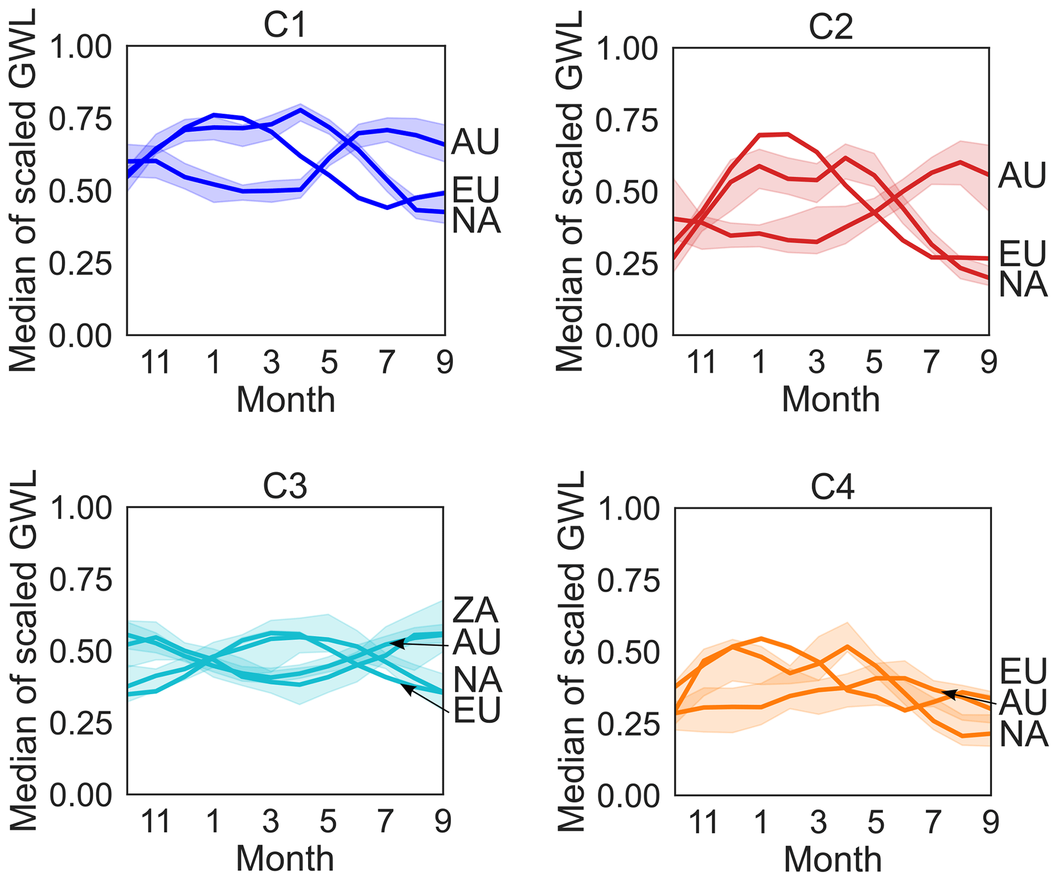
Figure 2 Annual hydrographs (median and 95 % confidence interval) from averaged groundwater depths of scaled GWL time series for each month per cluster, calculated and plotted for the coastal regions in North America (NA), Europe (EU), South Africa (ZA), and Australia (AU) when at least 10 time series associated with the respective cluster were available.

GWLs in three out of four clusters can be located either mostly at their upper (CL1) or lower (CL4) boundary during the year, with high GWLs in winter and spring to low GWLs in summer, or the GWL fluctuates around its annual median during the year, with high interannual amplitude (CL2). In contrast, GWLs of CL3 are characterized by maximum water levels being reached later in the year.

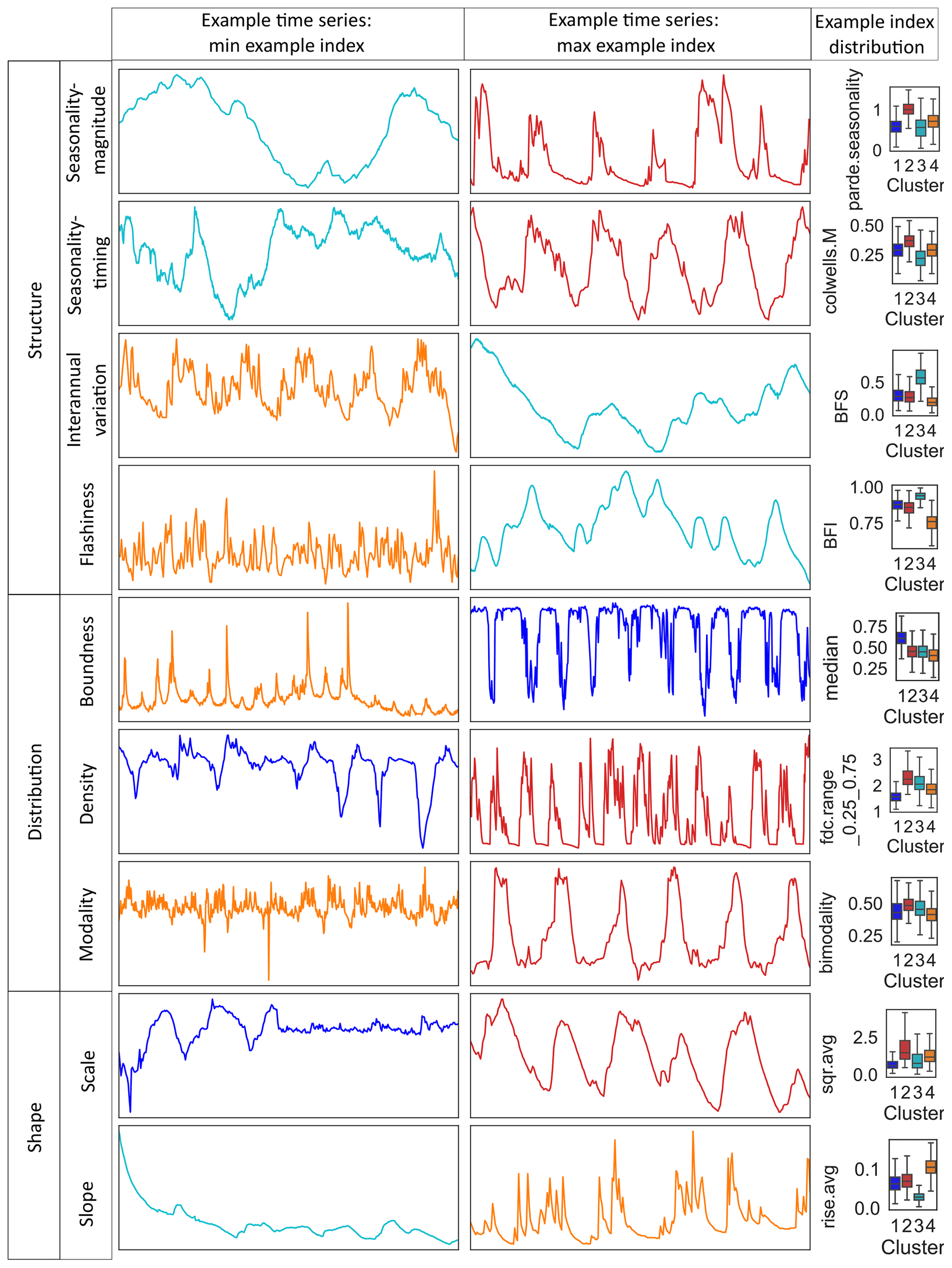
Figure 3 Example groundwater time series from the European continent illustrate typical scaled GWL time series where one aspect from each component of the Heudorfer et al. (2019) typology of GWL dynamics (Table B1) is weak (left column) and one is strong (right column), with an example index from that component that is displayed showing within-cluster variability (see Fig. C4 for within-cluster variability for all indices).

The clusters can be distinguished with respect to multiple features of the hydrograph, expressed by indices. Thus, the salient pattern of each cluster is defined by several indices and not by an individual one. However, some individual indices allow us to separate clusters or groups of clusters better than the others. Figure 3 shows how different aspects of GWL dynamics, each described by multiple indices (Table B1), contribute to disentangling patterns of GWL dynamics. Many indices of multiple components clearly separate clusters concerning the hydrograph structure, including the regularity of the seasonal amplitude (parde.seasonality) that is small for CL1 and CL3 and largest for CL2, the size of the global amplitude of the unscaled GWL that is comparatively small for CL4, the manifestation of interannual variation (e.g., from base flow stability (BFS) that implies that interannual variation is rather stable in CL3 and unstable in CL4), and different orders of flashiness (e.g., from base flow index (BFI), where the base flow component is large for CL3 and small for CL4). From the time series distribution aspect, GWL dynamics from CL1 can be characterized as upper bounded, while GWL dynamics from CL4 are slightly lower bounded (e.g., from median). Dispersion over the range of GWLs (e.g., from the range of duration curve (fdc.range) between different percentiles) is smallest in CL1 and largest in CL2. The shape of GWL time series in terms of both scale (hydrograph magnitude (sqr.avg)) and slope (e.g., from rise.avg) distinguish the clusters quite well from each other. For example, CL3 is particularly noticeable for combining GWL time series with a small slope, while CL4 combines such with a large slope.

3.2 Classification of groundwater level dynamic patterns

In the classification task using RF, controls of GWL dynamics were investigated using more than 5000 unique cluster–attribute relationships. Stable classification accuracy during hyperparameter tuning was achieved with more than 100 trees. Both splitting criteria that were tested performed equally well in terms of classification accuracy, whereas the consideration of different features for the splits led to a significantly higher accuracy (Fig. D1). The final model of this study was set up using the Gini criterion, randomly varied subsets (square root) of features for each split, and 700 trees.

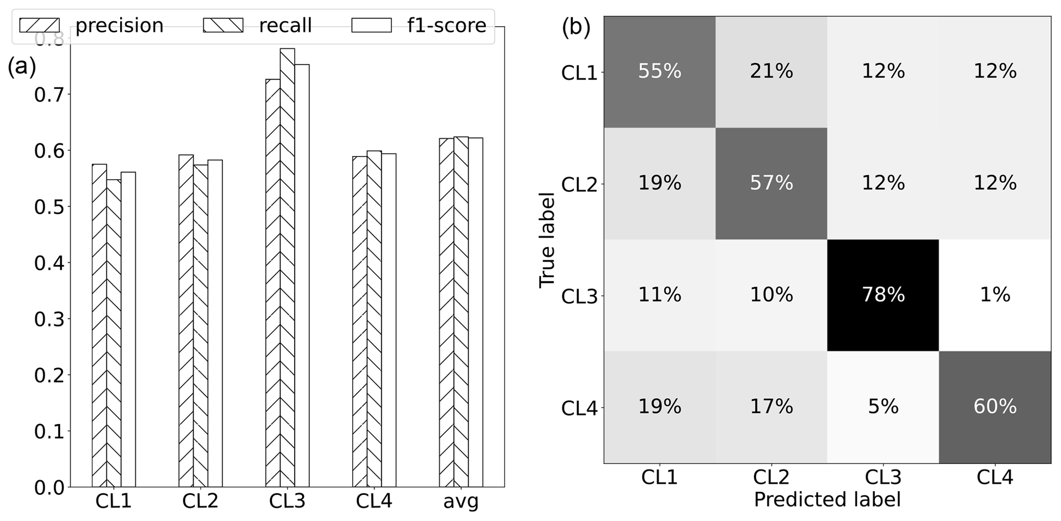
Figure 4 Performance of the classification task using random forest (Breiman, 2001). (a) Evaluation metrics of classification (precision, recall, and F1 score) given per cluster and for the weighted average (performance metrics weighted according to the support of each cluster). (b) Normalized confusion matrix. Rows represent the actual cluster, while columns represent the predicted cluster. Thus, the percentages of correctly predicted classes are represented by the diagonal elements, and the confusion (i.e., misclassification) is represented by the off-diagonal elements.

With the final model, approximately 62 % of the clusters, on average, were classified correctly; i.e., they were assigned to the correct cluster out of four. Comparing the model's result accuracy to a scenario where descriptors were shuffled shows an improvement in accuracy of about 60 %. By shuffling the attributes, the relationships between the descriptors and the target variable (clusters) are disrupted, and any observed accuracy in the shuffled model is purely due to chance. These results suggest the presence of moderately strong linkages between the attributes and clusters describing distinct GWL dynamic patterns within the RF model. Figure 4 shows that the classification performance is distributed partly unequally across the different clusters. From the confusion matrix, it can be seen that CL3 is most often (78 %) predicted correctly and, if not, is either confused with CL1 or CL2 but almost never with CL4. The other clusters are predicted correctly similarly often, with accuracies ranging from 55 % to 60 %. Recall and precision of the clusters are quite similar. Considering the slightly different support of each cluster, the classification performs, on average, similarly well in terms of false-positive cluster assignments (e.g., a well site is classified as CL1 when it actually belongs to another cluster) and false-negative assignments (e.g., a well site that belongs to CL1 is not classified as CL1 but as another cluster). Overall, there are only minor differences in classification performance among the various coastal regions.

3.3 Model explanations from SHAP values

SHAP values that were calculated for the classification model are used in the discussion to explain the importance and effects of different controls on GWL dynamics, while general results for the RF model are presented here.

By analyzing the correlation of SHAP values, we can detect where feature importance may be affected by information redundancy (Fig. E1). In this study, the redundancy among features tends to be small or moderate, and patterns are not very consistent across the clusters. Specifically, the redundancy between feature groups (in correspondence with categories of attributes in Table 1) is minimal for cluster CL3 in the model, whereas it is more evident for cluster CL4. CL2 exhibits redundant contributions from anthropogenic features and features derived from surface waters, with climate features being additionally redundant in the prediction of cluster CL1.

Three groups of features are ranked higher in terms of overall feature importance in the global model compared to the remaining three groups (Fig. E2). These are topography and subsurface depths, followed by soil and lithology and climate, with only minor differences in the importance of the features between the clusters. The largest difference is that the feature group of topography and subsurface depths is about twice as important in the model for predicting CL3 compared to the other three clusters. For these clusters, the feature groups of soil and lithology and climate are similar in importance compared to topography and subsurface depths. Therefore, features of the group of topography and subsurface depths primarily play a role in distinguishing CL3 from the other clusters.

Table 2 Qualitative description of the more important and, in their effects, more differentiable features, starting with the feature group with the greatest importance for the model (Fig. E2) and for the prediction of the individual clusters in comparison based on Fig. E3; < and > mark smaller and larger feature values for one or more clusters compared to one or more other clusters, while there is no clear information for –. ^∗ Aridity index: see Table 1.

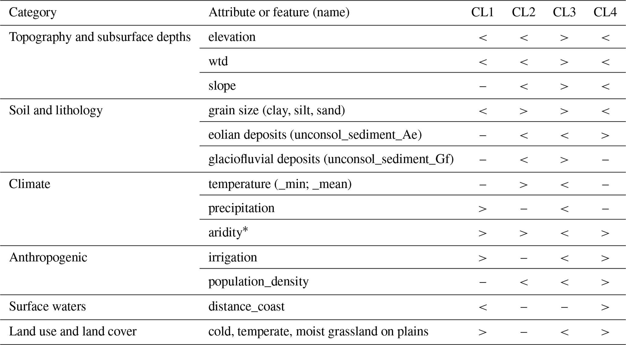
More in-depth insights into how the model can distinguish the clusters – and, in particular, CL1, CL2, and CL4 – from each other through the various features can be derived when using SHAP values to link the feature impacts to their effects (Table 2, Fig. E3). From the individual features, elevation, slope, and water table depth (wtd) are most important within the feature group of topography and subsurface depths; soil fractions and the (non)occurrence of specific unconsolidated sediments are most important within the feature group of soil and lithology; temperature is most important within the feature group of climate; irrigation is most important within the feature group of anthropogenic; distance to the coast is most important within the feature group of surface waters; and the (non)occurrence of a specific terrestrial ecosystem type is most important within the feature group of land use and land cover. The most significant effects that features have on predicting clusters in the RF model are those that best separate clusters from each other (Table 2). CL3 is best distinguished from the other clusters by a comparatively large elevation, large wtd, and large slope. In addition, some effects specifically separate (a) CL3 from CL4, (b) CL4 from CL1 and CL2, and (c) CL1 from CL2, although the latter is the least successful in the model (largest confusion values of CL1 and CL2 in Fig. 4). In comparison with CL2, CL3 combines well locations with lower minimum and average temperatures and sediments typical for glaciofluvial deposits. In comparison with CL1, CL3 combines well locations with less precipitation, more coarse-grained soils, and less anthropogenic activity. Feature effects between CL3 and CL4 are most often contrary, although they are less pronounced for climate. Where CL2 is predicted, there are also comparatively more coarse-grained soils and rarely sediments typical for eolian deposits, and anthropogenic activity is low. These characteristics from soil and lithology, as well as anthropogenic activity, also separate CL4 from CL2. Less differentiates CL4 from CL1. It is noticeable that the distance of the well to the coast is generally higher in CL4 compared to CL1. The typical well locations in CL1 and CL2 differ in their soil fractions (finer-grained soils in CL1) and anthropogenic activity (larger in CL1).

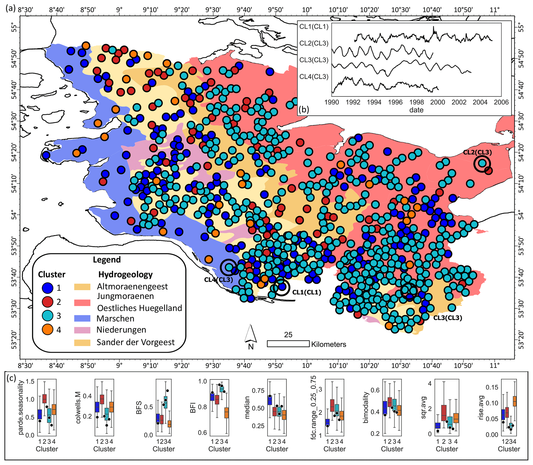
Figure 5 GWL dynamic patterns in the German federal state Schleswig-Holstein. (a) Cluster assignment to well locations and hydrogeology map of the German federal state Schleswig-Holstein (LfU-SH, 2003). Overlapping well markers are jittered at a minimum spacing of 500 m and thus no longer represent the original well locations. The cluster number in parentheses marks the true cluster from k-means clustering. (b) Exemplary time series of each cluster from the encircled well sites in (a). (c) Within-cluster variability of the example indices that each represent a component of the Heudorfer et al. (2019) typology from Fig. 3, plotted with index values (dots) of the encircled well sites in (a), where the dots between CL2 and CL3 and between CL4 and CL3 mark the wells that have the highest probability for CL2 and CL4 in the RF model but belong to CL3 according to the clustering (see Fig. C5 for within-cluster variability for all indices that are plotted together with index values of the selected well sites).

Finally, SHAP values for individual wells that are all located in the same region in northern Germany (Fig. 5) can be used to understand how the results of the feature importance and effects derived from the global dataset apply regionally. We analyzed the SHAP values of four well sites from the case study region that have the highest probability of being predicted by the model for each cluster in the test dataset (Figs. E4–E7). The wells that are most likely to be predicted as CL1 and CL3 are also included in these clusters, whereas the wells that are most likely to be predicted as CL2 and CL4 are part of CL3. Thus, although CL3 is overall the best-identified cluster by the model (Fig. 4), in the case study region, where most of the wells belong to CL3, it is confused with CL2 and CL4 for the example wells. The correct prediction of CL1 is due to the low elevation and wtd at the well location, as well as the presence of grassland (Fig. E4). Due to these characteristics, the well is also not predicted to be CL3, while the region's mean temperatures around 10 °C also favor CL3 at this well site. The statistically averaged temperatures, which should be very constant for the region, can sometimes favor and sometimes disfavor all clusters. According to local feature importance in this region, temperature is the most important attribute following elevation and wtd for the prediction of GWL dynamic types at specific wells. However, when analyzing SHAP values for a model trained on a global dataset, we are primarily examining the global context for a local feature, not the local context. Besides confirming temperature, CL3 is correctly predicted where its prediction probability is largest because of comparably large elevation in the study region and because there is no irrigation (Fig. E6). In contrast, a CL3 well is incorrectly predicted as CL2 with low elevation and a population density that is below average for the region (Fig. E5). Another CL3 well is incorrectly predicted as CL4 with low elevation and one of the highest clay contents for the region (Fig. E7). The described relationships are in line with or not contradictory compared to the global correlations of Table 2.

4 Discussion

4.1 Hydrogeological similarity and scaling effect

Four predominant types of GWL dynamics were identified for coastal wells distributed across five continents. Our results show that shallow aquifers exhibit more diverse GWL dynamics than deeper aquifers. This suggests that absolute GWL depth is less determinant in differentiating global GWL dynamics than might be assumed based on the clustering of direct time series from a single particular region, as in Rinderer et al. (2019), where, in particular, mean water level and amplitude of variation determine clusters of GWL dynamics.

Based on the spatial distribution of clusters, wells exhibit distinct regional structures that strongly imply the presence of underlying spatial controls; e.g., CL3-type GWL dynamics in northern Germany tend to coincide with Geest land, while CL1-type GWL dynamics are more often found in the marshlands (Fig. 5a). Another example is that the topographically elevated Veluwe region in the center of the Netherlands is the only region at the North Sea where many wells are assigned to CL3 (Fig. 1). However, GWL dynamics of different types are also frequently found in wells within a very short distance from each other or even on top of each other (in the case of multiple groundwater storeys). This means that the diversity of GWL dynamics can be larger locally than between two wells in different climate zones on different continents, likely due to the significant influence of heterogeneous hydrological conditions. Therefore, in addition to the findings by Wunsch et al. (2021), it is shown that nearby wells do not necessarily have a higher degree of similarity in terms of GWL dynamics compared to more distant wells – even when these wells are located on different continents. Regionally similar but locally diverse GWL dynamics highlight the complexity of generalizing GWL dynamics on different spatial scales. Yet, the fact that our results include spatial patterns at local, regional, and global scales (considering the globally distributed clusters of GWL dynamic types) points to the usefulness of our approach in finding generalizations beyond specific geographic contexts. We therefore conclude that our approach is robust with respect to scale dependency. Previously, studies on GWL dynamics have resulted in systemic understanding at local and regional scales (Wunsch et al., 2021; Giese et al., 2020; Haaf et al., 2020). While this may be more straightforward for applied groundwater management and monitoring at these scales, this study is the first to provide insights into generalizations of GWL dynamics using a global dataset.

We found that using indices for analyzing GWL dynamics is efficient and offers comparability and interpretability. In these terms, this approach might be superior compared to directly analyzing GWL time series or only focusing on the long-term mean or trends. Heterogeneous time series with different seasons, time series lengths, and periods can be combined in this approach with robust results, as previous studies have shown (Heudorfer et al., 2019; Wunsch et al., 2021), thereby reducing the dimension of the time series and potentially better establishing cause-and-effect relationships. From the clustering results, we can see that indices successfully separate between climatic forcing (as present in seasonality) and physiographic forcing, while in practice, it remains challenging to identify what drives GWL dynamics at various scales and settings (Blumstock et al., 2016; Moeck et al., 2020) and to distinguish between the impacts of climatic and other natural factors versus anthropogenic impacts on GWL dynamics and trends (Wriedt, 2017; Lischeid et al., 2021). Although indices are affected by the length of the GWL time series (Heudorfer et al., 2019), they can help to identify time series with “high-amplitude, low-frequency variability”, such as in Normandy (Paris Basin, France; compare Baulon et al., 2022b). Groundwater well sites with dominant interannual variations from multi-annual to decadal scales identified by Baulon et al. (2022b) in this area match well sites with CL3-type GWL dynamics found in this study (Fig. C6). At these well sites, the likelihood of approaching short-term groundwater drought is higher if the prevailing low-frequency variability is associated with a downward phase, while the annual GWL status and the previous winter's groundwater recharge have less influence on short-term drought (Baulon et al., 2022b). Overall, we can therefore assume that longer residence times are typical characteristics for CL3-type aquifers.

The methodological approach underlying the GWL dynamic analysis offers much potential but also has limitations and uncertainties with respect to the validity of the generalizations generated. Despite the fact that general robustness of indices was found starting at time series with a minimum length of 4 years (Heudorfer et al., 2019), uncertainties remain regarding the representativeness of the generalizations for individual wells with this time series period length but less so for the generalizations themselves. Furthermore, Heudorfer et al. (2019) originally defined some of the indices for time series with daily resolution, and decadal GWL dynamics are only indirectly represented by indices in our study (e.g., seasonality in the annual hydrograph). Therefore, further investigation of the effects of different temporal resolutions and time series lengths, as performed in Papacharalampous et al. (2023) for hydroclimatic time series, would be of interest. With respect to the groundwater systems and processes represented by the GWL dynamic patterns, it should be emphasized that there may be a bias in favor of the typical GWL dynamics in northwestern Europe because most of the wells in the dataset are located there.

Classification of specific groundwater processes requires input data specifically related to and known to be influential in relation to these processes. However, there are major limitations with available GWL data, particularly in terms of time series length and data resolution. GWL time series are rarely sufficiently long to recognize the dimension of climate change, making it difficult to establish an effective monitoring and management strategy. High-resolution time series are, for example, required for analyzing the interaction of groundwater with the sea (Haehnel et al., 2023). Accounting for SWI in GWL dynamic pattern analysis is best supported by pattern recognition or correction together with groundwater chemistry data (Narvaez-Montoya et al., 2023; Parisi et al., 2023). However, the expansion of studies on this topic is currently hampered by the lack of GWL time series with high temporal resolution, as well as the lack of availability of qualitative groundwater data together with GWL data, among other challenges in groundwater monitoring practice (Rau et al., 2020). Several studies have shown the degradation of groundwater in qualitative and quantitative terms due to its overexploitation (Alfarrah and Walraevens, 2018; Peters et al., 2022; Xanke and Liesch, 2022), but it was beyond the scope of this study to focus on changes in groundwater systems. Furthermore, more in-depth analyses of the individual indices could help to find out to what extent and in which indices specific processes such as SWI or anthropogenic influence are manifested and thus contribute to a classification.

The index-clustering analysis conducted in this study was instrumental in capturing the major patterns of GWL dynamics of coastal regions worldwide. The utilization of the k-means algorithm has enabled us to represent these patterns at a high level, providing valuable generalizations. However, if in other research questions the necessary level of pattern recognition is smaller, clustering algorithms that do not require both clearly distributed data and clearly defined clusters have the potential to identify additional clusters and uncover more nuanced dynamics within the dataset.

4.2 Cause-and-effect relationships

We further analyzed whether the identified types of GWL dynamics are meaningful, i.e., consistent with expected patterns (Yang and Chui, 2021), although machine learning can also reveal undetected and previously unexplained patterns. We generally expect patterns as a result of the multitude of natural and anthropogenic factors influencing GWL dynamics. Meaningful GWL dynamics have the potential to derive cause-and-effect relationships between GWL dynamics and their driving forces, a topic for which observation-based evidence is comparatively scarce. Thus, in this study, driving forces were linked to GWL dynamic patterns in an RF classification task. Here, many different environmental attributes describing surface and – to a smaller extent – subsurface processes potentially associated with groundwater recharge and discharge were used to explain (dis)similarities within and between the identified patterns.

While comparing individual aspects of the hydrograph with potential controlling factors can only explain specific aspects of GWL dynamics (e.g., Haaf et al. (2020) related flashiness (BFI) to focused recharge as a consequence of depressions or connectivity to streams), the holistic analysis of various GWL dynamic aspects against controls enables the estimation of the influence of multiple controls over processes defining groundwater quantity over time.

Since GWL dynamics in coastal regions can be similar in different regions globally, similar GWL dynamics are not necessarily the result of the same cause-and-effect relationships. Rather, it can be expected that there are complex interlinkages of multiple controls that favor hydrogeological similarity in different manifestations of the individual attributes. We, therefore, confirm our initial expectation that similar GWL dynamics derived from indices are associated with multiple processes and, vice versa, that the important controls and processes can be identified and distinguished by a combination of indices. This is in line with previous findings with hydro-climatic time series (McMillan, 2020; Beck et al., 2016).

The results show that relationships between GWL dynamic patterns and controls can be generalized to the global scale to some extent. Notably, the importance of different attribute categories (Table 1, Fig. E2) for shaping GWL dynamics is related to hierarchical relationships where climate, topography, and soil conditions have a greater influence over the occurrence and characteristics of surface waters, as well as of land use and land cover, than the other way around. This implies that the direct influencing factors offer more explanatory power. Then again, direct influencing factors in the attribute dataset are more often based on actual observations and often have a higher resolution (e.g., the minor explanatory power of attributes from surface waters might also be related to a coarse spatial resolution of about 55 km). From the importance of elevation and water table depth, especially for the determination of CL3-type dynamics and differentiation from other dynamics that are more often found in near-surface aquifers, it can be concluded that these attributes mainly describe the increasing damping effect of groundwater recharge with increasingly long soil passages. The generally high importance of climatic attributes for GWL dynamics – either only in the long term or also in short periods – is scientific consensus, making climate change a usual part of assessments of changes in groundwater systems (Riedel and Weber, 2020). Also, within the group of climatic attributes, the importance of direct attributes such as temperature outweighs derived attributes such as the aridity index. According to Table 2, certain types of unconsolidated sediments and a terrestrial ecosystem can distinctly indicate or exclude specific GWL dynamic types. These manifestations of categorical attributes are likely to serve as proxies for the general importance of their class. Due to the multitude of manifestations, only the most common ones are likely to appear in the importance ranking in Fig. E3 (e.g., eolian deposits mainly exist in the Netherlands, which also provides the most wells in the dataset).

Anthropogenic activities such as irrigation and groundwater pumping typically have a localized effect. They have the potential to overprint different types of GWL dynamics even when the hydrogeological setting is the same (Sorensen et al., 2021). Together with small-scale lithological and hydrogeological peculiarities, they likely contribute the most to the variability of GWL dynamic patterns locally and regionally. Section 4.1 emphasizes the importance of the data basis, including its current limitations, for assessing certain processes. From the comparably minor importance of anthropogenic attributes for GWL dynamics, it could be assumed that global groundwater quantity is less influenced by anthropogenic than by natural controls. On the one hand, this was also the expectation with using data derived from monitoring networks and after quality control. On the other hand, it is unclear how much of the explanatory content of the anthropogenic attributes is based on anthropogenic activities and how much is due to correlations with natural controls (Fig. E1). Such interactions could be that irrigation is higher in dry climates and that there are more sealed surfaces where population density is high. Therefore, anthropogenic impact is also difficult to disentangle from natural controls in this study.

Moderate accuracy of the RF model means that parts of the GWL dynamics derived from indices are not well predicted based on the used attributes. Hence, machine learning tools that are trained to find cause-and-effect relationships face the same challenge of process-based groundwater models: limited availability and quality of explanatory data, especially subsurface information. Even if there is great progress in the availability and quality of geoscientific data, surface attributes derived for the global scale are still biased by uncertainty in the data itself (Peng et al., 2017), by coarse spatial resolution, and by the period they cover. In the presented approach, no dynamic attributes were used because they are not available for all attribute categories at the global scale. For instance, land use has a large influence on the water balance with land use conversion (Mishra et al., 2014). The fact that explanatory information is missing in the RF model for differentiating GWL dynamics at the local to regional scale can be observed, for example, in the case study region in northern Germany (Fig. 5). Furthermore, as explained in Sect. 2.4, studies of global scope, such as this one, face limitations in accurately defining subsurface catchments.

4.3 Case study

Finally, the question also arises as to what extent it is possible to explain the generalized GWL dynamics derived with the index-clustering approach of this study regionally if attributes were only good enough. The inclusion of regional context using the case study from northern Germany (Fig. 5) serves a dual purpose in our study. First, in Sect. 4.1, we assessed the robustness and validity of our proposed approach for identifying GWL dynamics at different scales. In this section, the case study serves as a critical test bed for understanding the chances and limitations of extrapolating explanations for patterns of GWL dynamics from the global to the regional scale. This case study was selected because a hydrogeological map and related hydrogeological information exist (LfU-SH, 2003), the GWL time series source dataset includes information on the aquifer storey of the wells, the well density is high, and the accuracy of the RF model is about the same in this region as it is globally. These conditions allow the study of spatial patterns and the ground-truthing of the GWL dynamic patterns using expert knowledge.

To a large extent, the near-surface aquifer in this area is a pore aquifer of silicate type formed during the Ice Age (LfU-SH, 2003; Otto, 2001). The hydrogeological situation of the shallow groundwater can broadly be divided from west to east into three major landscapes: (a) low-lying marshlands (Marschen); (b) slightly raised Geest landscapes (Altmoraenengeest), the lower outwash plain (Sander der Vorgeest), and intervening depression zones comprising the river valleys (Niederungen); and (c) morainic uplands with stronger relief (Jungmoraenen Oestliches Huegelland).

GWL dynamics in the marshlands predominantly belong to CL1 (59 %), especially in the upper two aquifer storeys (68 %) and close to the sea, followed by CL3 (20 %), which combines more GWL dynamics of the lower aquifer storeys (60 %) and well sites at the border of the Geest. The Geest and uplands are characterized by GWL dynamics that mainly belong to CL3, with some exceptions, including the Geest landscape in the north close to the Danish border (GWL dynamics are of mixed type), the area around the major depression in the north (GWL dynamics mainly belong to CL1), and the eastern uplands at the southernmost bay (GWL dynamics mainly belong to CL1). In the lower Geest, GWL dynamics belong to CL2 (23 %) more often than in other landscapes. As in the marshlands, CL3-type GWL dynamics are associated more often with lower aquifer storeys compared to the other clusters in these areas (63 %–78 %), with the difference being that CL3 is also present to a similar degree in the upper aquifer storeys in the Geest and uplands (45 %–67 %). Figure 5b displays example time series of wells that the RF model identifies as having the highest probability for each cluster. The cluster in parentheses indicates the actual cluster that is based, among others, on the index values shown in Fig. 5c. In cases where CL3 was mistaken for CL2 and CL4, the example wells mostly have indices within the CL3 distribution (Fig. 5c). While there are minimal visual differences in the time series between CL2 and CL3 at the well location where CL2 is predicted, some distinctions can be observed in Fig. 5b when CL3 is misidentified as CL4.

The inability of the RF model to correctly predict these instances can therefore mainly be attributed to two factors. First, the GWL dynamics at the predicted wells for CL2 and CL4 reside closer to the border between different dynamic types, making them more challenging to differentiate. This is confirmed by some very similar index values compared to CL3. Second, the limited explanatory potential provided by the attributes can be assumed to also contribute to the model's failure: expert information suggests that small-scale differences in GWL dynamics in the case study region can be explained by lower aquifer storeys with good hydraulic connections to upper storeys and surface waters. The presence of both CL1 and CL3 dynamics in the higher Geest and upland regions, regardless of groundwater storey, can be attributed to differences in the soil covering, water table depth, and the existence of both unconfined and confined upper aquifers in these landscapes (LfU-SH, 2003). Comparing the ground-truthing with the RF model, some global explanations apply to this regional context as well. For instance, in the marshlands and the northern depression zone, where impermeable sediments of small to medium thickness overlay the aquifer (LfU-SH, 2003), the prevalence of CL1 and CL4 type wells is higher (Table 2).

5 Conclusions

In summary, this study provides new insights into the hydrogeological behavior and the hydrogeological similarity in coastal regions. It utilizes an unprecedented dataset of GWL time series and demonstrates the development of a global information archive on GWL dynamics for high-level generalizations. These findings can aid in developing broader frameworks for effective groundwater management – for example, by identifying regions with common characteristics and highlighting essential hydrograph features for global modeling. Our results show that hydrogeological similarity is a global phenomenon that, with respect to the aquifers near the coastline, can be divided into four clusters representing distinct patterns of GWL dynamics. Similar clusters are observed globally across different continents and climate zones, while GWL dynamics can be highly variable regionally and locally, suggesting a complex interplay of controlling factors. Therefore, extrapolating GWL dynamics from a single well to the surrounding area may sometimes be less appropriate than inferring GWL dynamics from global relationships. However, establishing global dynamics–control relationships remains a challenge. We found that these are mainly dominated by (a) topography and groundwater depth, mainly determining the responsiveness of groundwater systems to impacts on the water cycle that separates well a single cluster from three others, and (b) climate and soil characteristics, which differentiate these three clusters with high short-term and interannual variability. However, groundwater management typically requires a more precise explanation of GWL dynamics by controlling factors beyond what is currently achievable with the attribute data available at the global scale. In particular, disentangling anthropogenic impacts from natural controls in GWL dynamics, e.g., to accurately predict the effects of climate change on GWLs without incorrectly accounting for water withdrawals, is of great importance for sustainable groundwater management. While the overall importance of anthropogenic activities to GWL dynamics was found to be smaller compared to natural characteristics in this study, more in-depth analyses were beyond the scope of this study. When analyzing certain processes, including SWI, it is important to pay attention to the data basis (selection of groundwater data and indices). To address the explanatory limitations of data-driven analysis and the prediction of GWL dynamics, we suggest using attributes closely related to actual observations and the direct influencing factors in combination with explainable machine learning techniques and suggest relying more on groundwater hydrographs and derived indices when attribute data are scarce or associated with large uncertainties. Overall, machine learning techniques combined with hydrograph information show promise for improving our understanding and predictive capabilities in addressing GWL complexities, especially at large spatial scales.

Appendix A: Groundwater data

Table A1 List (country-wise, alphabetical) of governmental agencies or portals from which groundwater data were obtained.

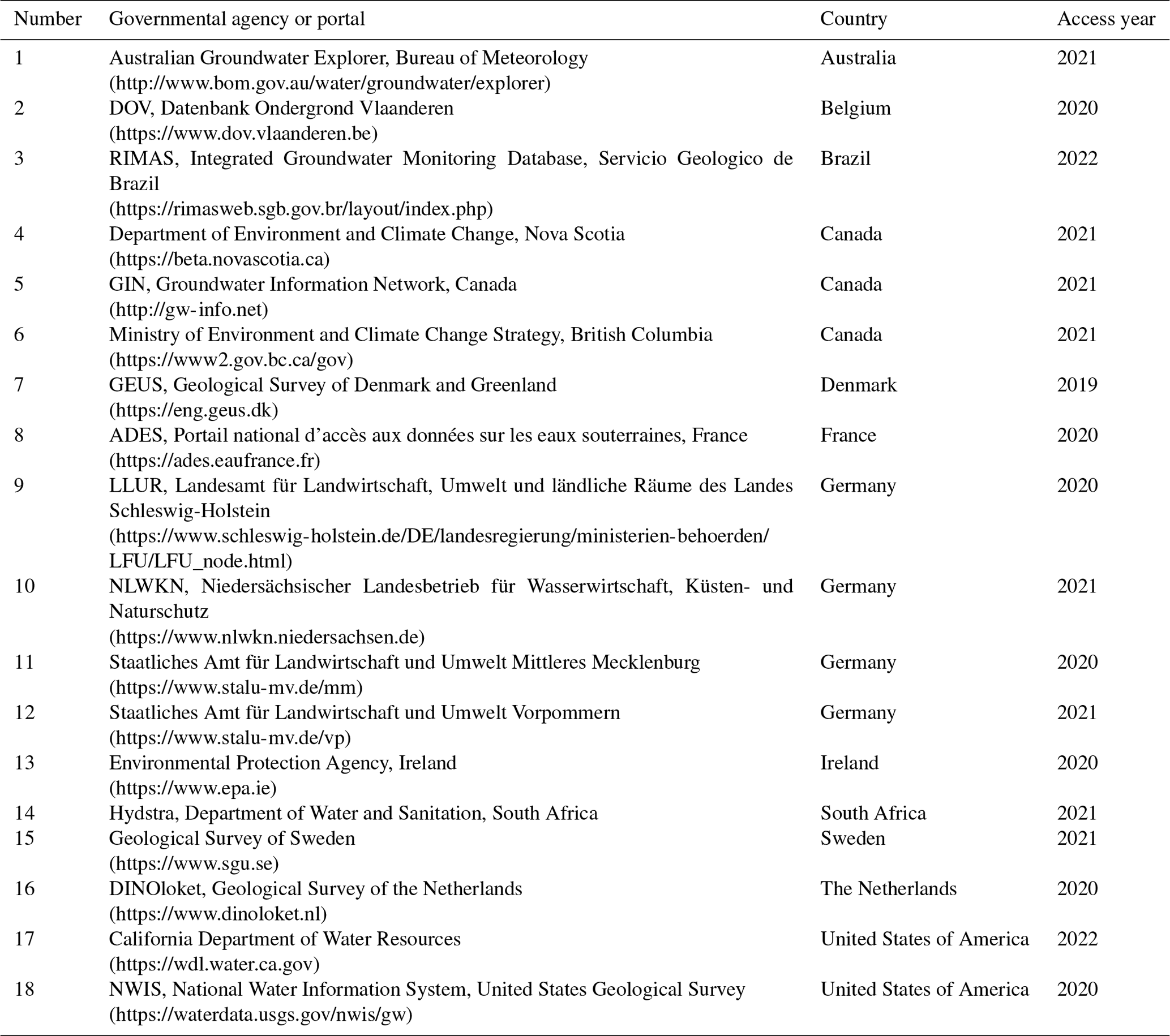
The last access date for all links is this table is 6 March 2024.

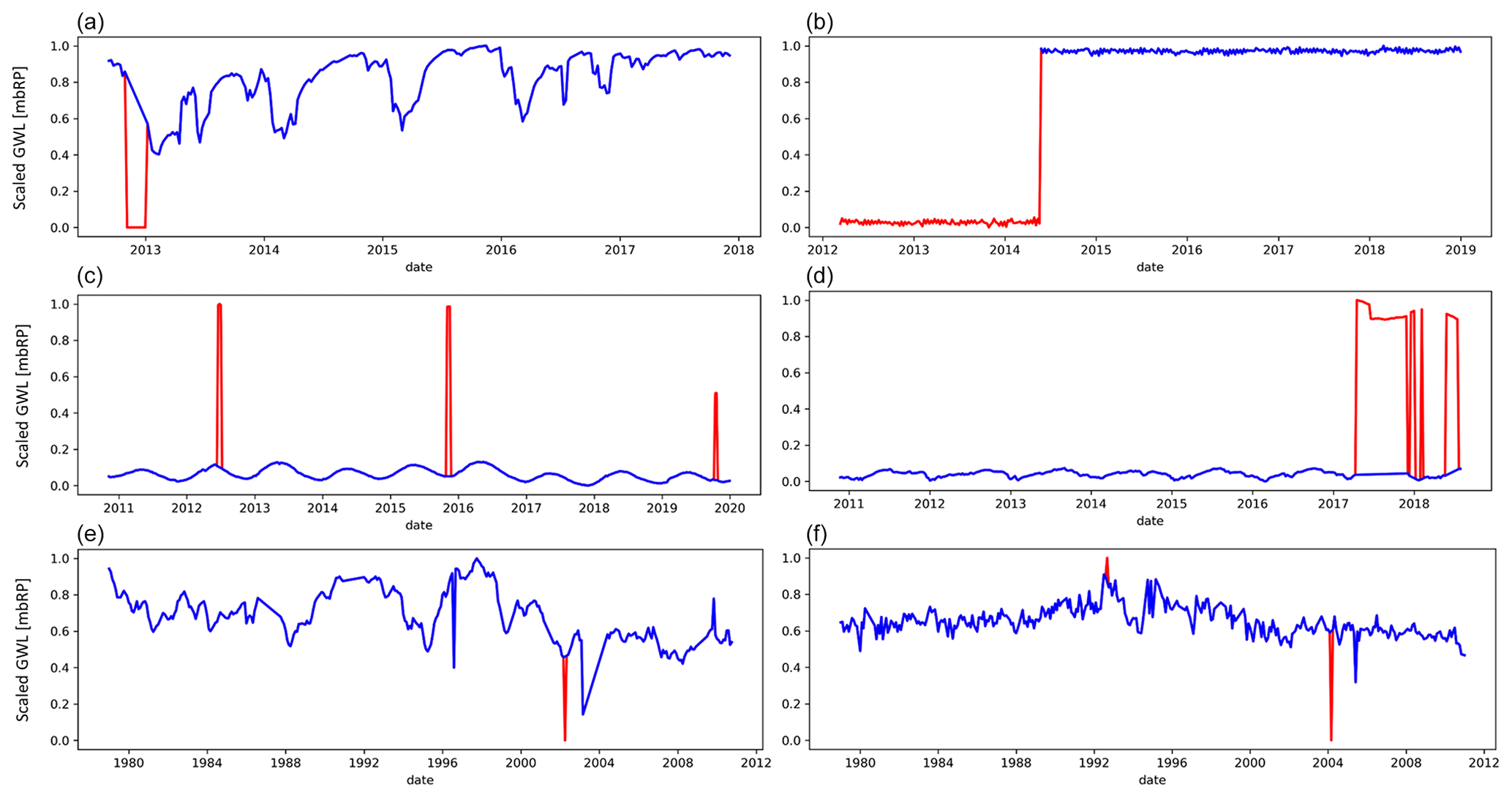
Figure A1 Examples of time series outlier removal with DBSCAN (scikit-learn library in Python): raw (scaled) time series are shown in blue, and the anomalies identified by DBSCAN (Ester et al., 1996) are shown in red. The use of DBSCAN is less successful or difficult to verify in the bottom two examples (in panel e, the first abrupt change in direction of the GWL between 1996 and 2000 is not identified as an outlier, although one would expect one based on the magnitude and position of the change; in panel f, from visual inspection, it is unclear whether the identified outliers in both directions are due to measurement error or human activity or reflect natural behavior of the groundwater system, e.g., extreme events). In summary, like other tested outlier detection methods, DBSCAN does not allow us to detect all types of outliers and anomalies that we would expect should be removed to represent undisturbed GWL dynamics. With the parameters set, we can successfully detect most density-dependent outliers, but many values were incorrectly identified as outliers. Therefore, we performed a visual inspection of all time series where DBSCAN identified potential outliers.

Appendix B: Indices

Table B1 List of GWL dynamic typology and indices used in this study. Differing names in brackets refer to deviating abbreviations in Heudorfer et al. (2019).

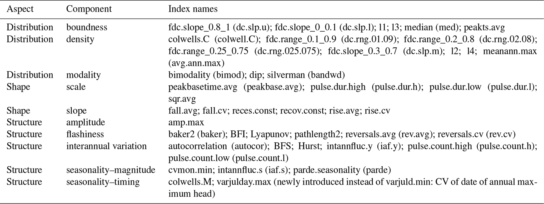
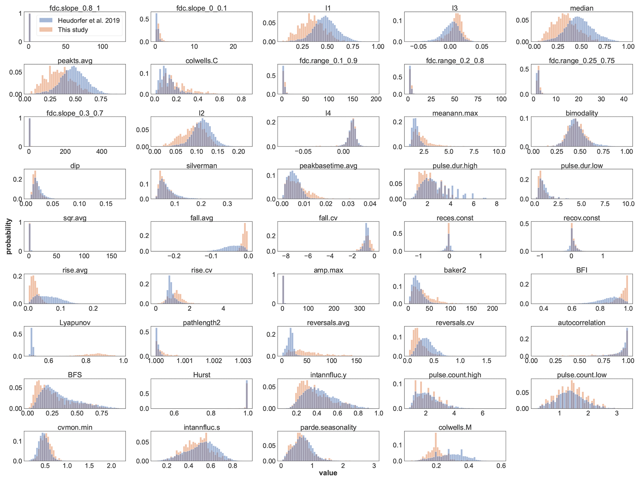
Figure B1 Comparison of the value distributions of the indices calculated in this study (Table B1) with the values published by Heudorfer et al. (2019) (dataset: Haaf and Heudorfer, 2018). The magnitude and variability of values for many indices are similar. Shifted or significantly different ranges of values are observed for some indices. Such differences exist for indices of different aspects of the hydrograph (structure, distribution, and shape).

Figure B2 Correlation matrix of the index values calculated in this study.

Appendix C: Clustering

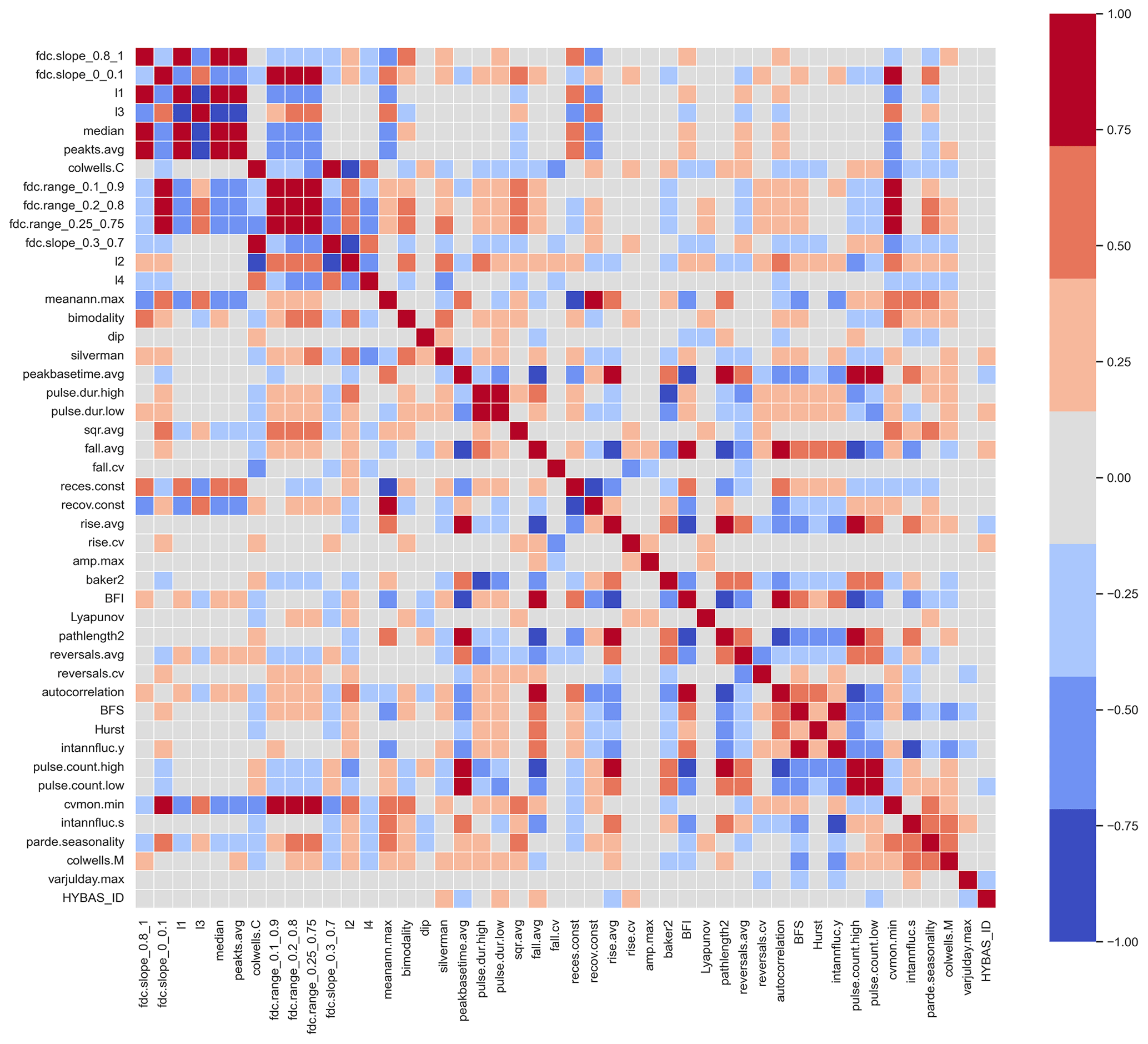
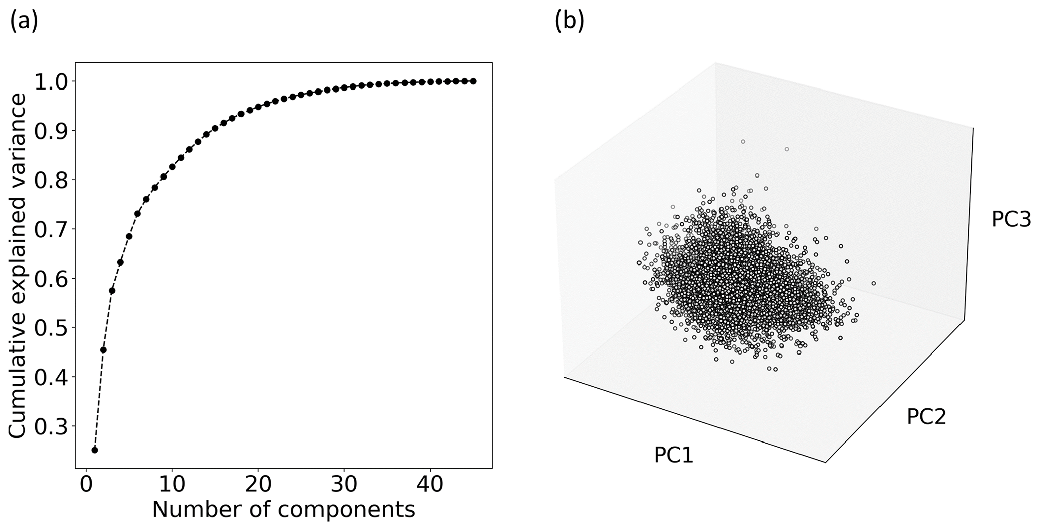
Figure C1 Principal component analysis with the index dataset. (a) Cumulative explained variance with an increasing number of principal components (PCs). (b) Dataset value space of the first three PCs (which together explain more than 50 % of the variance of the dataset).

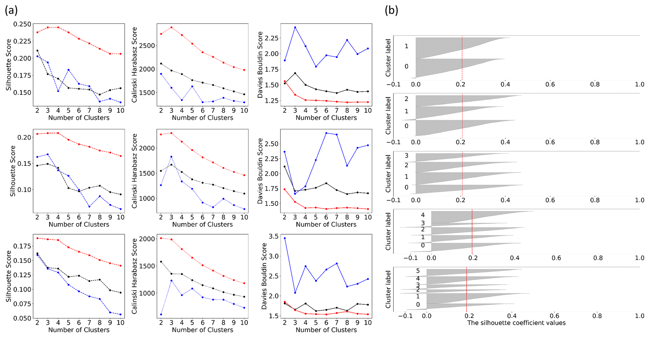
Figure C2 Evaluation metrics – Silhouette (Rousseeuw, 1987), Calinski–Harabasz (Caliński and Harabasz, 1974) and Davies–Bouldin (Davies and Bouldin, 1979) – used to find the best cluster separation. The Silhouette score ranges from −1 to 1, where a higher value indicates better-defined clusters. Better clustering results are also indicated by higher values for the Calinski–Harabasz score and by lower values for the Davies-Bouldin score. (a) Metrics are shown for different proportions of explained variance represented by principal components (PCs) (top to bottom row: 60 %, 70 %, and 80 %) and for different clustering algorithms (k-means clustering, red; Gaussian mixture, blue; and hierarchical clustering, black). (b) Silhouette scores for various clusters using the k-means algorithm and PCs representing 70 % of explained variance.

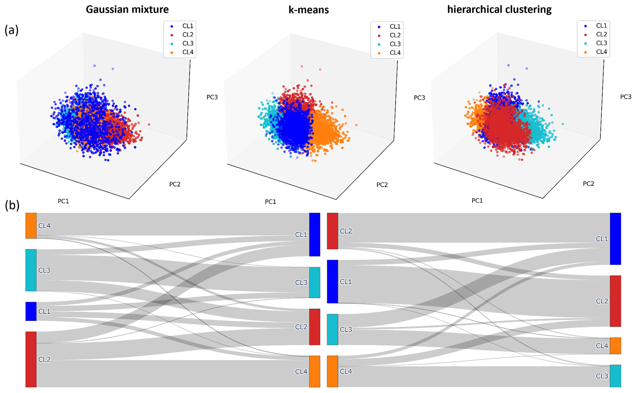
Figure C3 Assignment of the time series to four different clusters by three algorithms (Gaussian mixture, k-means clustering, and hierarchical clustering). (a) Illustrative cluster assignment within the range of values of the first three principal components (PCs) of the dataset. (b) Sankey plot allows comparison of the quantitative distribution of the samples among the clusters (left between Gaussian mixture and k-means clustering and right between k-means clustering and hierarchical clustering).

Figure C4 Within-cluster variability of all indices used for clustering.

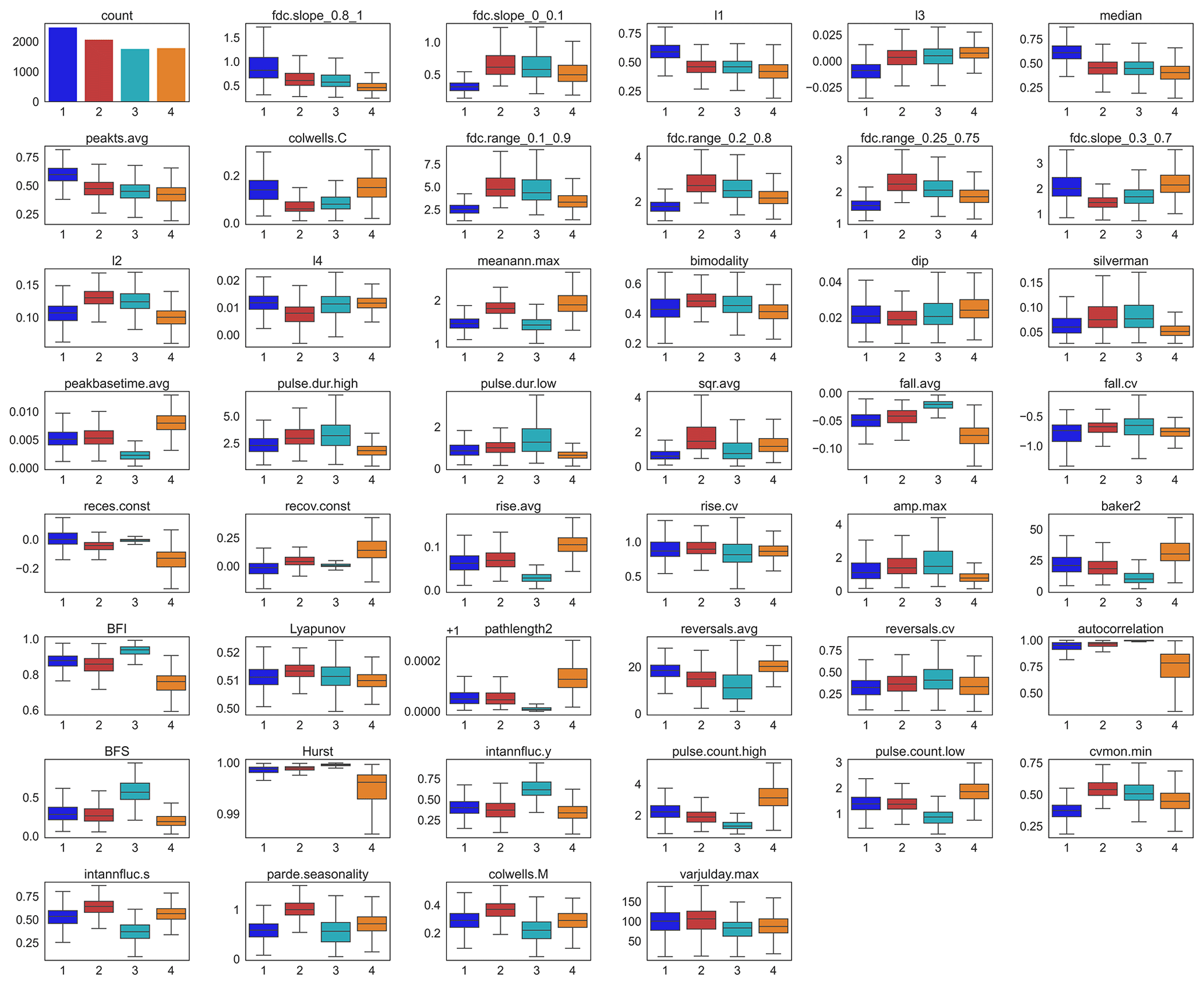
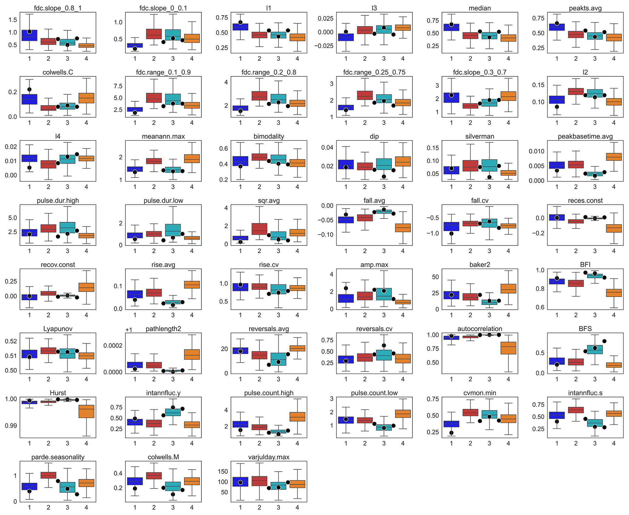
Figure C5 Within-cluster variability of all indices used for clustering (Fig. C4) plotted with index values (dots) of the four example wells from the case study region in northern Germany (Fig. 5a). The points drawn between CL2 and CL3 and between CL4 and CL3 are wells with the highest probability for CL2 and CL4 in the random forest model but that belong to CL3 according to the clustering.

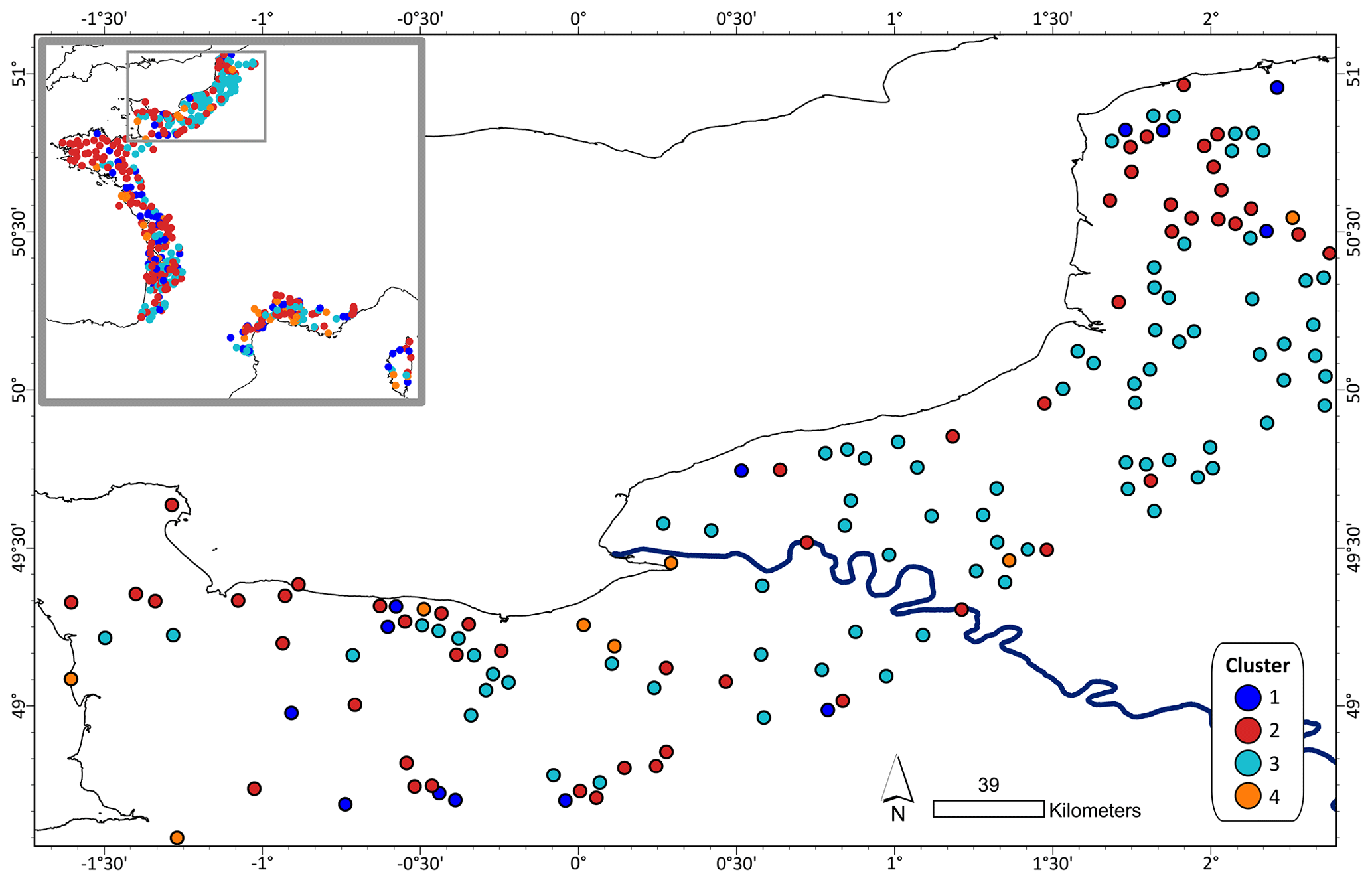
Figure C6 Assignment of clusters to well locations in Normandy, Paris Basin, displayed with the Seine River. Overlapping well markers were jittered at a minimum spacing of 1000 m and thus no longer represent the original well locations. The window in the upper-left corner shows the Normandy region in the north of France.

Appendix D: Random forest classification

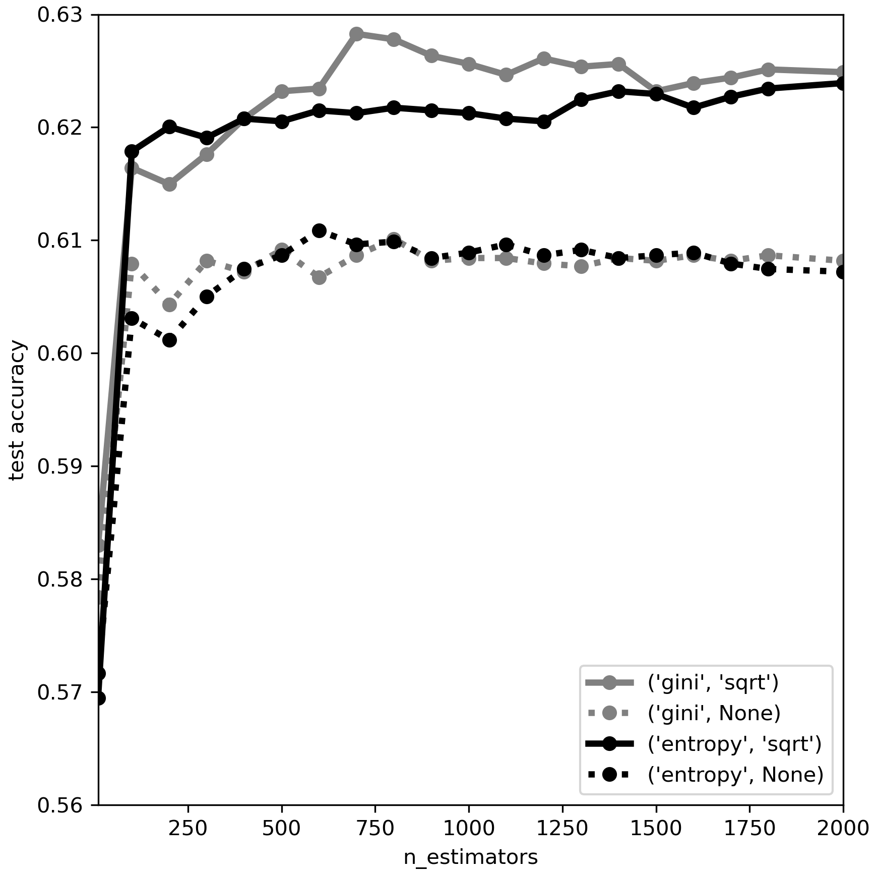
Figure D1 Random forest hyperparameter tuning within a 5-fold cross-validation framework using the training data.

Appendix E: SHAP

Figure E1 Absolute Spearman correlation of SHAP values for aggregated features (SHAP values added up for features from the same attribute categories from Table 1).

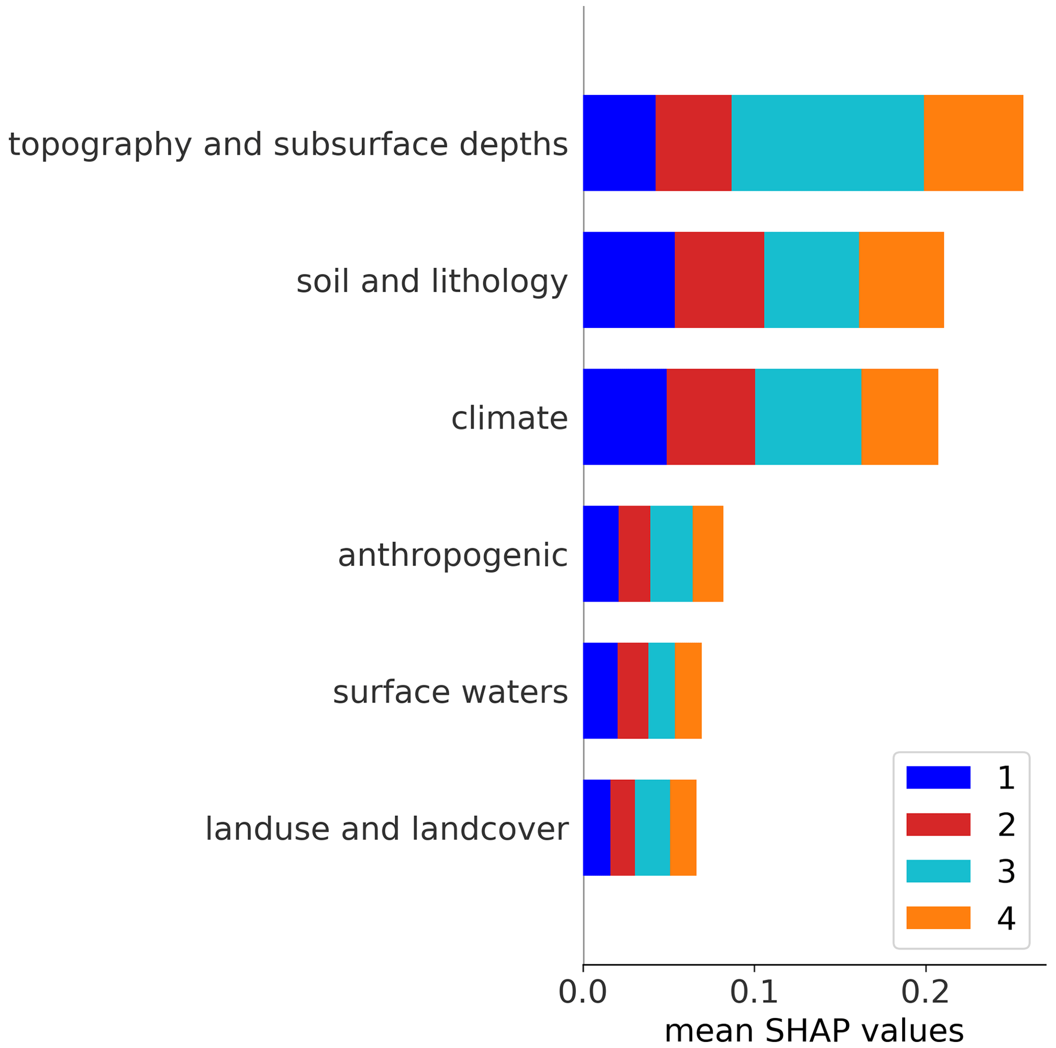
Figure E2 Overall SHAP feature importance stacked for individual clusters for aggregated features (SHAP values added up for features from the same attribute categories from Table 1).

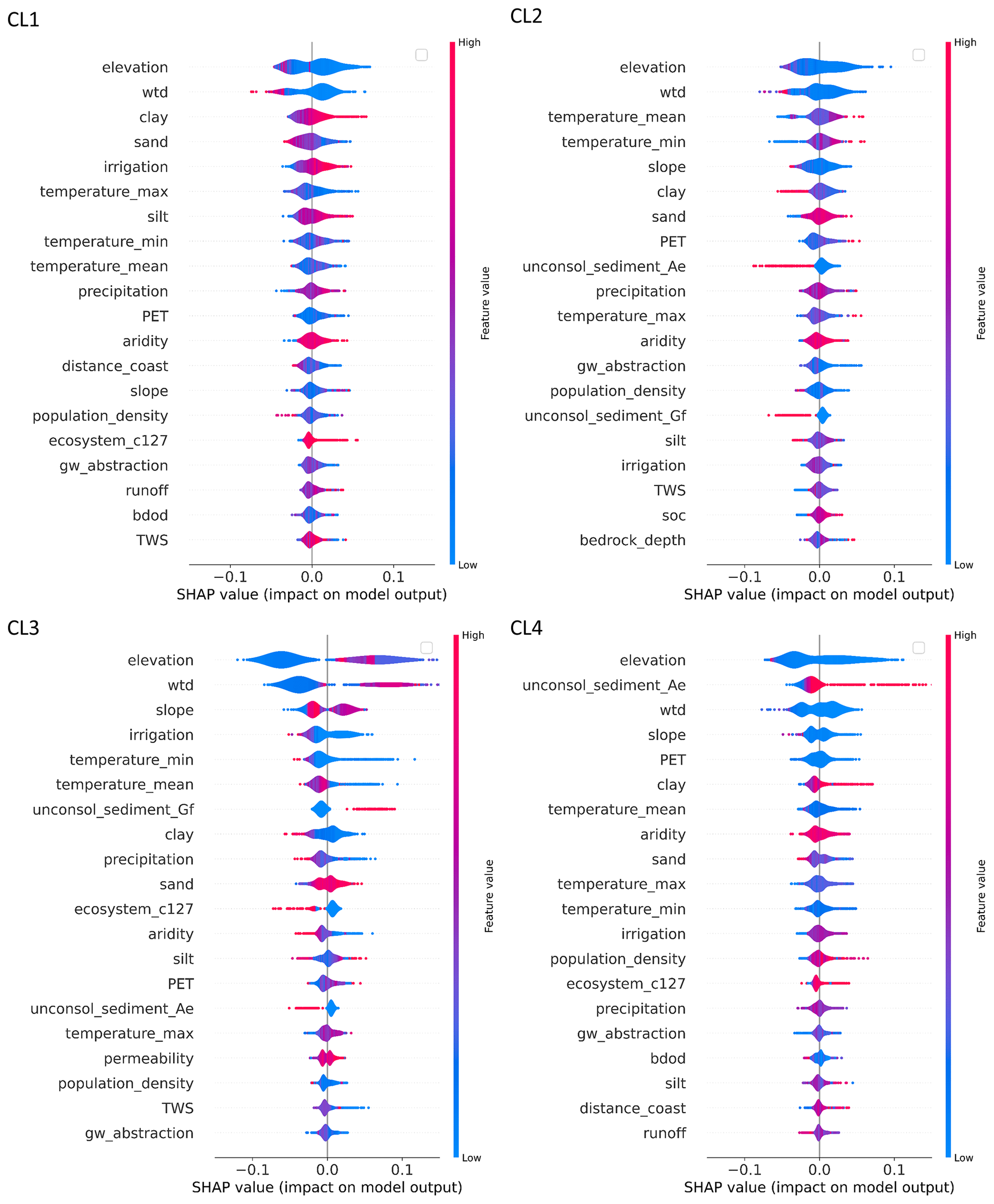
Figure E3 Violin plots show the distribution of SHAP feature importance and feature effect for the 20 highest-ranked features of each cluster. SHAP values describe the impact of a given feature on the prediction of the model for a given cluster (the prediction of true for the selected cluster). A red color corresponds to high feature values, and a blue color corresponds to low feature values (for one-hot-encoded features, a value of 0 (blue) corresponds to the presence of the feature class, and a value of 1 (red) corresponds to the absence of the feature class). Overlapping instances widen the violin shape in the direction of the y axis, and the violin at that position is colored according to the average feature value.

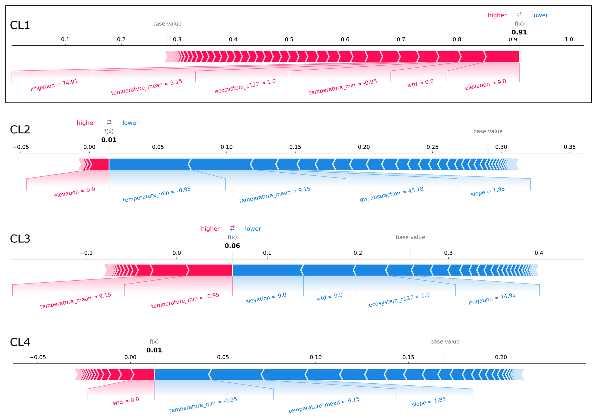
Figure E4 SHAP force plots explaining the correct prediction of the CL1 exemplary well site from the case study region in northern Germany (Fig. 5a). At this well site, the probability that CL1 is predicted is the largest in the case study (test dataset). The average scores of all classifications made by the random forest model for the training dataset are 0.28, 0.29, 0.26, and 0.17 (base values). The model's probability scores for predicting the clusters at the exemplary well site (bold-printed numbers) sum up to 100 %. Features that are important for the respective predictions are displayed with their values. Their importance and effect can be assessed by the SHAP values visualized by bar length and color (i.e., the larger the feature's share of the bar, the more important; red represents rejecting effect, and blue represents supporting effect).

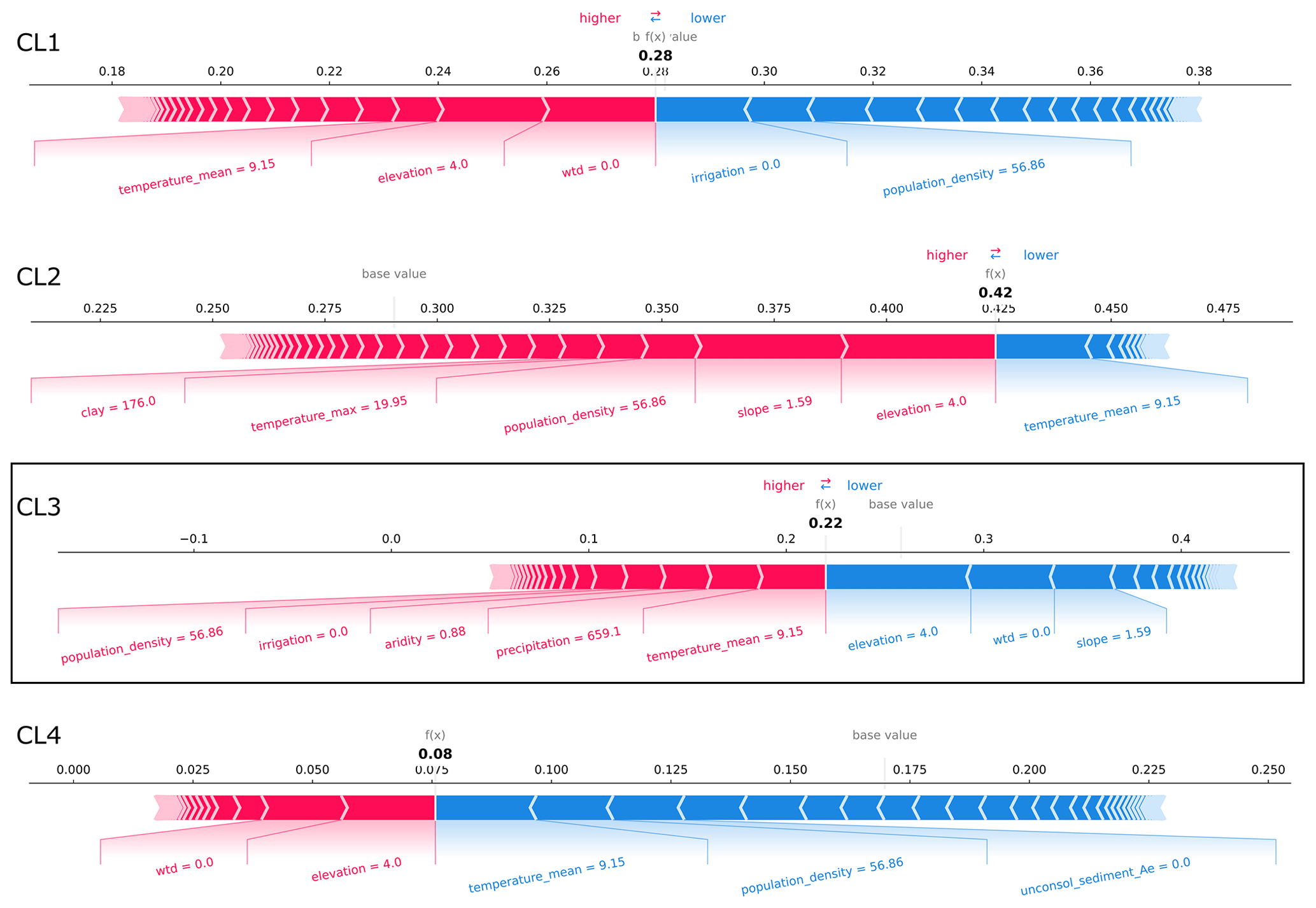
Figure E5 SHAP force plots explaining the prediction of the CL3 exemplary well site from the case study region in northern Germany (Fig. 5a) that is confused with CL2. At this well site, the probability that CL2 is predicted is the largest in the case study (test dataset). The average scores of all classifications made by the random forest model for the training dataset are 0.28, 0.29, 0.26, and 0.17 (base values). The model's probability scores for predicting the clusters at the exemplary well site (bold-printed numbers) sum up to 100 %. Features that are important for the respective predictions are displayed with their values. Their importance and effect can be assessed by the SHAP values visualized by bar length and color (i.e., the larger the feature's share of the bar, the more important; red represents rejecting effect, and blue represents supporting effect).

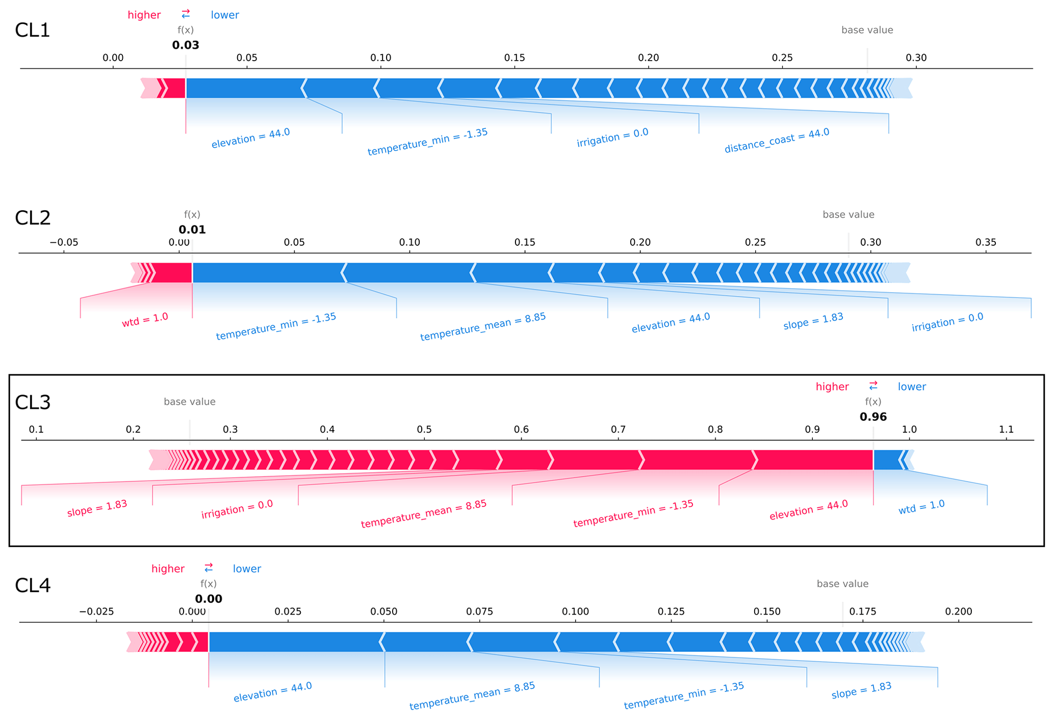
Figure E6 SHAP force plots explaining the correct prediction of the CL3 exemplary well site from the case study region in northern Germany (Fig. 5a). At this well site, the probability that CL3 is predicted is the largest in the case study (test dataset). The average scores of all classifications made by the random forest model for the training dataset are 0.28, 0.29, 0.26, and 0.17 (base values). The model's probability scores for predicting the clusters at the exemplary well site (bold-printed numbers) sum up to 100 %. Features that are important for the respective predictions are displayed with their values. Their importance and effects can be assessed by the SHAP values visualized by bar length and color (i.e., the larger the feature's share of the bar, the more important; red represents rejecting effect, and blue represents supporting effect).

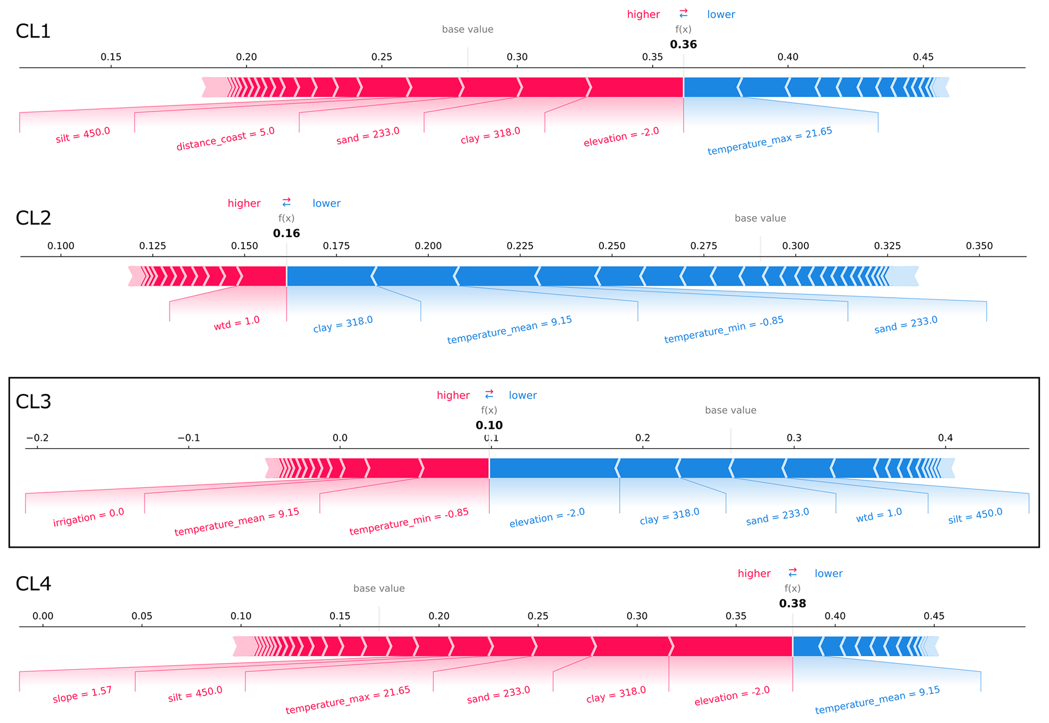
Figure E7 SHAP force plots explaining the prediction of the CL3 exemplary well site from the case study region in northern Germany (Fig. 5a) that is confused with CL4. At this well site, the probability that CL4 is predicted is the largest in the case study (test dataset). The average scores of all classifications made by the random forest model for the training dataset are 0.28, 0.29, 0.26, and 0.17 (base values). The model's probability scores for predicting the clusters at the exemplary well site (bold-printed numbers) sum up to 100 %. Features that are important for the respective predictions are displayed with their values. Their importance and effects can be assessed by the SHAP values visualized by bar length and color (i.e., the larger the feature's share of the bar, the more important; red represents rejecting effect, and blue represents supporting effect).