On optimization of calibrations of a distributed hydrological model with spatially distributed information on snow

In northern cold-temperate countries, a large portion of annual streamflow is produced by spring snowmelt, which often triggers floods. It is important to have spatial information about snow variables such as snow water equivalent (SWE), which can be incorporated into hydrological models, making them more efficient tools for improved decision-making. The present research implements a unique spatial pattern metric in a multi-objective framework for calibration of hydrological models and attempts to determine whether raw SNODAS (SNOw Data Assimilation System) data can be utilized for hydrological model calibration. The spatial efficiency (SPAEF) metric is explored for spatially calibrating SWE. Different calibration experiments are performed combining Nash–Sutcliffe efficiency (NSE) for streamflow and root-mean-square error (RMSE) and SPAEF for SWE, using the Dynamically Dimensioned Search (DDS) and Pareto Archived Dynamically Dimensioned Search multi-objective optimization (PADDS) algorithms. Results of the study demonstrate that multi-objective calibration outperforms sequential calibration in terms of model performance (SWE and discharge simulations). Traditional model calibration involving only streamflow produced slightly higher NSE values; however, the spatial distribution of SWE could not be adequately maintained. This study indicates that utilizing SPAEF for spatial calibration of snow parameters improved streamflow prediction compared to the conventional practice of using RMSE for calibration. SPAEF is further implied to be a more effective metric than RMSE for both sequential and multi-objective calibration. During validation, the calibration experiment incorporating multi-objective SPAEF exhibits enhanced performance in terms of NSE and Kling–Gupta efficiency (KGE) compared to calibration experiment solely based on NSE. This observation supports the notion that incorporating SPAEF computed on raw SNODAS data within the calibration framework results in a more robust hydrological model. The novelty of this study is the implementation of SPAEF with respect to spatially distributed SWE for calibrating a distributed hydrological model.

1 Introduction

Cold-temperate countries like Canada are characterized by substantial spring runoff, where streamflow is generated or amplified by snowmelt. Indeed, spring snowmelt is one of the predominant hydrological events influencing the annual water budget of high-latitude watersheds (DeWalle and Rango, 2008; Buttle et al., 2016). Rapid melting of snow can result from a combination of high temperatures and rainfall over frozen ground resulting in heavy runoff, which will exacerbate flooding. A reliable flow forecast system, therefore, should provide inflow forecasts using hydrological models that can simulate the complex processes occurring in the watershed. These models can mimic the relationship between inflow and outflow in a watershed provided that they have adequate meteorological data (precipitation, temperature, relative humidity, and wind speed and direction) and geographical data (digital elevation model, land cover and soil maps) (Singh and Woolhiser, 2002). Distributed hydrological models are capable of representing the spatial variability of hydrological processes and state variables within a watershed, which cannot be obtained by lumped models (Markhali et al., 2022).

Snow distribution, together with the frequency, duration and intensity of spring snowmelt, influences extreme runoff events (Marsh et al., 2008), soil water storage capacity, subsurface flow (Roach et al., 2011; Frampton et al., 2013; Jafarov et al., 2018) and groundwater recharge (Mohammed et al., 2019; Ala-Aho et al., 2021). Owing to the dominant control of snow on the water balance during the snowmelt season, typically from March to May, the spatial distribution of snow has received much attention (Hiemstra et al., 2002; Woo and Young, 2004). Spatial variability of snow cover results from various processes that occur across different spatial scales (Clark et al., 2011). At the watershed scale, it is affected by meteorological variables (e.g., temperature, precipitation, evaporation) and by elevation, topography and vegetation, while at the hillslope scale it is governed by processes such as drifting, trapping of snow and nonuniform snow unloading by the forest canopy (Hojatimalekshah et al., 2021). Methods that are available for analyzing spatial variation of the snowpack have their limitations, and incorporating them into hydrological models is difficult. For example, interpolation techniques (Harshburger et al., 2010) for generating snow water equivalent (SWE) maps at the watershed scale require a surface network of ground SWE measurements, which are frequently limited in number or are absent. Passive microwave sensors provide appropriate information on snow in areas with simple topography, but they do not work properly in higher elevations, typically underestimating SWE (Wrzesien et al., 2017). Moreover, their low spatial resolution requires appropriate downscaling approaches to bring the information to the watershed scale. GlobSnow (Luojus et al., 2020), which is currently available as a global snow monitoring system, integrates passive microwave remote sensing data from multiple satellites to provide near-real-time information on snow cover extent at a global scale. This valuable resource offers insights into the spatial distribution of snow cover across diverse regions. On the one hand, and despite its easy accessibility, GlobSnow exhibits relatively coarse resolution (25 km × 25 km), thereby limiting its ability to capture fine-scale details. On the other hand, SNODAS (SNOw Data Assimilation System) (NOHRSC, 2004) represents a subsequent advancement that integrates passive microwave remote sensing data, ground measurements and weather data to generate gridded snow datasets at a finer resolution (1 km ×  1 km). The incorporation of various data sources and assimilation techniques into SNODAS enhances the quality and reliability of snow data, enabling more accurate hydrological modelling and facilitating rigorous scientific investigation.

SNODAS is a modelling and data assimilation system that had been developed by NOHRSC (National Operational Hydrologic Remote Sensing Center). It uses a physically based mass and energy balance snow model that assimilates automated ground and airborne measurements and satellite data (Zahmatkesh et al., 2019) to provide accurate estimates of snow cover and associated variables for hydrological modelling and analysis. The dataset includes snowpack properties such as depth and SWE, covering variables such as liquid precipitation, snowmelt runoff and temperature (Barrett, 2003). It has provided daily, gridded data at a 1 km × 1 km spatial resolution for the USA since 2004 and for southern Canada since 2009.

Researchers used bias-corrected SNODAS SWE data in hydrological modelling, given that it provides more accurate and reliable input data for the models whereas raw SNODAS data may contain errors and biases (Zahmatkesh et al., 2019; King et al., 2020). These errors and biases can adversely affect the accuracy of hydrological models that rely upon SNODAS data as input. A study by Clow et al. (2012) concluded that SNODAS provides reasonably true estimates of SWE in forested areas and can be used as observed data to calibrate hydrological models for moderate to large watersheds and for estimating runoff forecasts. Zahmatkesh et al. (2019) demonstrated that bias-correcting SNODAS SWE products, which align with the cumulative distribution function of interpolated SWE, improved the accuracy of the SNODAS products and enhanced model performance in simulating peak values during hydrological modelling and streamflow simulation. Despite the high uncertainty that is associated with SNODAS estimates in eastern Canadian watersheds, they remain valuable in regions with limited snow stations. Bias correction of SNODAS data may not be possible in situations where there is a lack of ground-based measurements or observations with which to compare the SNODAS data. Given the unavailability of observed SWE data in the study area, Leach et al. (2018) applied a bias correction technique, which was originally used for SNODAS snow depth data, to adjust the SNODAS SWE dataset, assuming a comparable level of relative bias between snow depth and SWE based upon their close relationship with the observations. This paucity of data compels researchers to explore new methods that allow the use of SNODAS data without relying upon traditional bias correction techniques.

This study addresses the need to investigate the feasibility and efficiency of employing raw SNODAS data for calibrating hydrological models without bias correction, utilizing diverse objective functions and evaluating the adequacy of the uncorrected SNODAS data in generating satisfactory results. The current research aims to bridge this gap by examining potential approaches that would enhance the reliability and accuracy of model outputs when working with raw SNODAS data, thereby contributing to the advancement of hydrological modelling techniques.

Distributed hydrological models, despite their capacity to mimic the spatial distribution of hydrological state variables and fluxes, continue to be used mainly for their temporal characteristics of the aggregated streamflow variable (Demirel et al., 2013; Schumann et al., 2013). Snow significantly influences the seasonal characteristics of streamflow, thereby affecting other hydrological processes, such as erosion, water supply and flood forecast. Given the importance of accurately representing snow processes in snow-dominated watersheds, hydrological model calibration should not solely focus on streamflow but should also account for snow dynamics (Troin and Caya, 2014; Hanzer et al., 2016; Tuo et al., 2018). Snow-related observations are frequently utilized to improve hydrological model performance through calibration experiments (Roy et al., 2010; Parajka and Blöschl, 2008; Di Marco et al., 2021). Hydrological model calibration in snow-dominated regions is complex because calibration based on snow variables does not necessarily lead to optimal parameters for streamflow and vice versa. Commonly used hydrological models can accurately replicate streamflow observations by calibrating them with respect to streamflow alone. However, they might struggle to properly capture state variables, particularly related to the snowpack (Duethmann et al., 2014; Casson et al., 2018; Liu et al., 2020; Thornton et al., 2021). For example, the models are usually calibrated using streamflow as the sole hydrological variable that is being simulated by the models, leaving other state variables, such as snow and soil moisture, unused in the calibration procedure. This is because spatially distributed observations traditionally have been difficult to obtain. To improve the reliability of hydrological models, it is critical to assess the simulated patterns of model state variables against spatially distributed observations. It is also important to ensure that the models can accurately reproduce the spatio-temporal dynamics of all relevant hydrological processes, leading to accurate streamflow forecasts (Kirchner, 2006).

The increased availability of remotely sensed observations has opened new doors in hydrological model calibration (e.g., snow cover, Terink et al., 2015; land surface temperature, Stisen et al., 2021). The objective of this research is to investigate strategies that include distributed snow information in the calibration of a distributed hydrological model, with a specific focus upon understanding the influence of different objective functions on the calibration process. The selection of an appropriate set of objective functions is crucial, as it introduces trade-offs among model parameters that influence overall calibration performance and model accuracy.

A number of temporal metrics are available for comparing simulated versus observed hydrographs, but spatial distribution comparison is occasionally used (Rees, 2008; Koch et al., 2018). Moreover, the spatial information that is contained in the observed data is not optimally utilized, given that the model parameters are constrained against spatial observations. Spatial metrics generally assess grid-to-grid correlation and deviations such as bias and Pearson’s correlation coefficient R. Demirel et al. (2018) developed a new spatial efficiency (SPAEF) metric with histogram matching to compare raster maps. The metric was later modified to include three different components, i.e., histogram intersection, variance and correlation, which offer bias-insensitive pattern information.

The primary objective in this study is to introduce spatial calibration with SWE data using newly developed metric SPAEF for the calibration of the HYDROTEL hydrological model. We applied SPAEF in combination with other traditionally used objective functions. We conducted seven distinct calibration experiments, each employing a unique combination of objective functions. This allowed us to assess the trade-offs and robustness of these various calibration scenarios by evaluating their performance in terms of both streamflow and spatial SWE patterns. Notably, while SPAEF has been previously applied in studies involving evapotranspiration (Demirel et al., 2018) and soil moisture (Eini et al., 2023), this study uses SPAEF with SWE for the first time.

2 Experimental setup

2.1 Study site

The Au Saumon watershed covers an area about 1120 km² and is located in the Éstrie region of Quebec (eastern Canada). It is a snow-dominated watershed that is subject to different climate conditions (summers tend to be warm and humid, with heavy rainfall; winters are cold and snowy; spring is the snowmelt season, with frequent rainfall; and autumn is drier with cooler temperatures). The watershed mostly has a rolling topography. Elevation ranges from 240 m at the watershed outlet, further rising up to 1100 m in the southern and eastern portions due to presence of Mont Mégantic (Fig. 1). This variation in elevation affects the spatial distribution of snow during winter, given that it affects temperatures. While rising to higher elevations, the temperature drops gradually, causing different patterns of melting and freezing in flat terrain and higher elevations. Vegetation cover in the watershed consists mainly of forests, i.e., 7 % conifer, 32 % deciduous and 45 % mixed forest. The remaining land cover consists of 9 % croplands; 2 % urban; and about 5 % wetlands, shrublands and grasslands (Fig. 1). Winter climate dominates this watershed, with snow cover usually forming in late November or early December and ending in April. Average minimum and maximum air temperatures during winter are −12 and −5 °C, respectively. Annual precipitation ranges from 1000 to 1200 mm (https://climate.weather.gc.ca/index_e.html, last access: 25 February 2024), with about one-third falling as snow (Bergeron et al., 2014). The parent material yields sandstone, limestone, and shale types of soils (silty loams) (https://sis.agr.gc.ca/cansis/, last access: 25 February 2024) (Seiller et al., 2012). There is one streamflow station (030282), as shown in Fig. 1 (https://www.cehq.gouv.qc.ca/hydrometrie/historique_donnees/, last access: 25 February 2024), with a drainage area of 769 km². There are no SWE data observation stations within the watershed; however, stations at Milan (station number: 302060) and Bury (station number: 302100) are located in close proximity to the watershed. These stations provide point data for SWE measurements (info-climat MELCCFP, 2020).

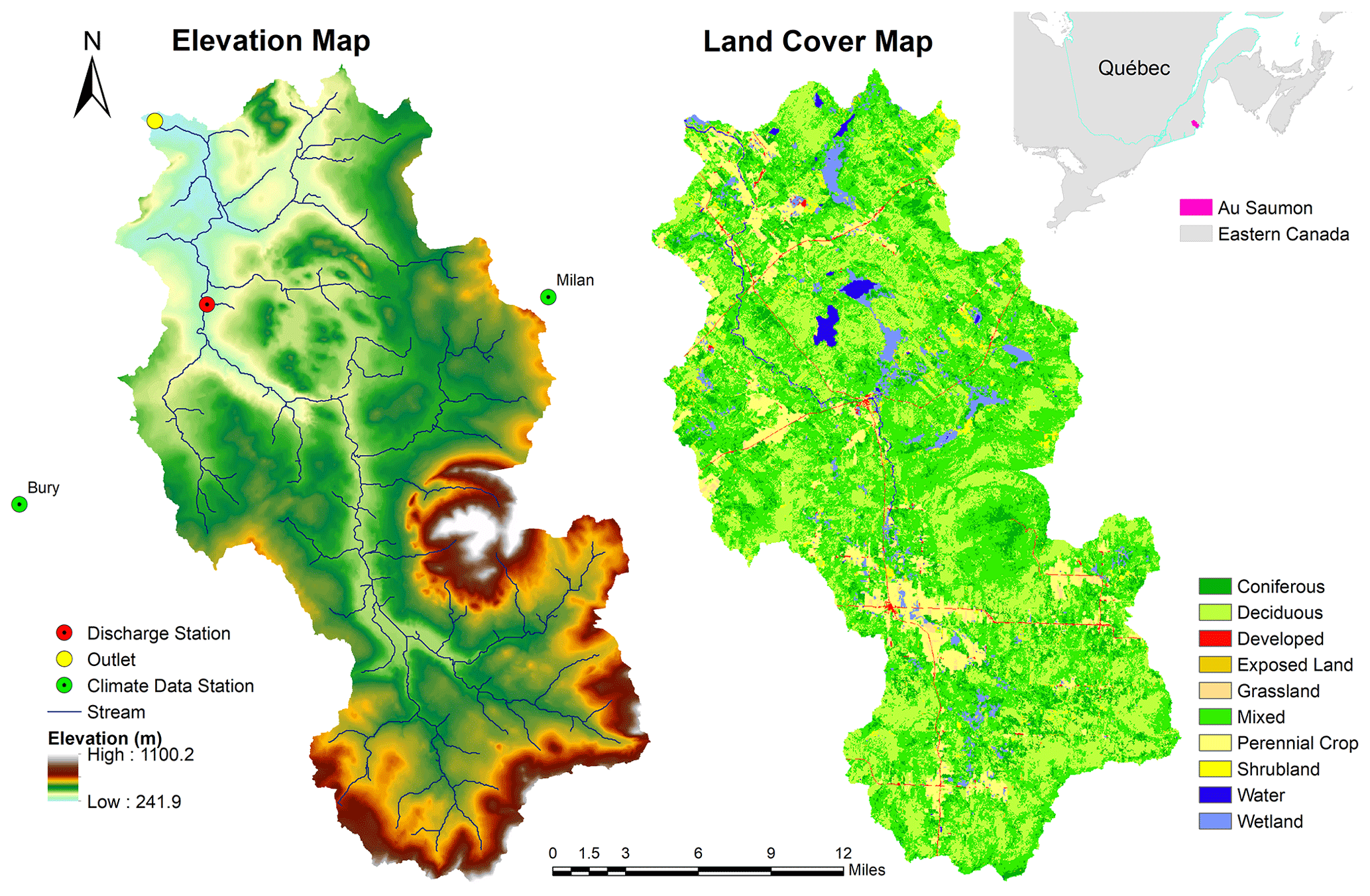
Figure 1 Au Saumon watershed location, elevation, stream network, streamflow outlet and land cover.

2.2 HYDROTEL model

The model that is selected for this study is a process-based, continuous, distributed hydrological model called HYDROTEL, which was developed by Fortin et al. (1995). The model has been used in a number of watersheds to study different hydrological processes, including variation of SWE (Turcotte et al., 2007; Oreiller et al., 2014; Fossey et al., 2016; Augas et al., 2020) and flow forecasting (Turcotte et al., 2004; Abaza et al., 2014, 2015). HYDROTEL serves as the base model for Quebec’s operational flow forecasting system. This model discretizes the watershed in several simulation units that are referred to as relatively homogeneous hydrological units (RHHUs) and river reaches (Turcotte et al., 2001). The characteristics of each RHHU depend upon land cover, soil types and topography (Rousseau et al., 2011). HYDROTEL can be simulated on a daily basis (opted for in this study) or in 3 h time steps. In our study, the Au Saumon watershed is subdivided into 205 RHHUs based upon the spatial distribution of land use, land cover, soil properties, slope and elevation. The mean surface area of the RHHUs is 4.5 km².

HYDROTEL is composed of different modules which run consecutively. The snow module uses a single-layer structure and is based upon a mixed degree day–energy balance hybrid approach. Snowpack characteristics (water equivalent, thickness, mean density, liquid water content, thermal deficit, temperature) are simulated using a modified energy budget approach that was developed by Riley et al. (1972). Empirical relationships are used to produce air–snow and ground–snow interface melt, albedo evolution, compaction, and the liquid water that is retained by the snow cover (Turcotte et al., 2007). The modules selected in this study are the Thiessen polygon method for interpolation of meteorological variables (with a vertical precipitation gradient of 1 mm per 100 m and a vertical temperature gradient of − 1 °C per 100 m), the Rankine method for soil temperature, the Thornthwaite equation for potential evapotranspiration and a three-layer model (BV3C) for the vertical water budget in the soil column. The output flow is simulated using the kinematic wave equation, and the model is simulated on a daily basis.

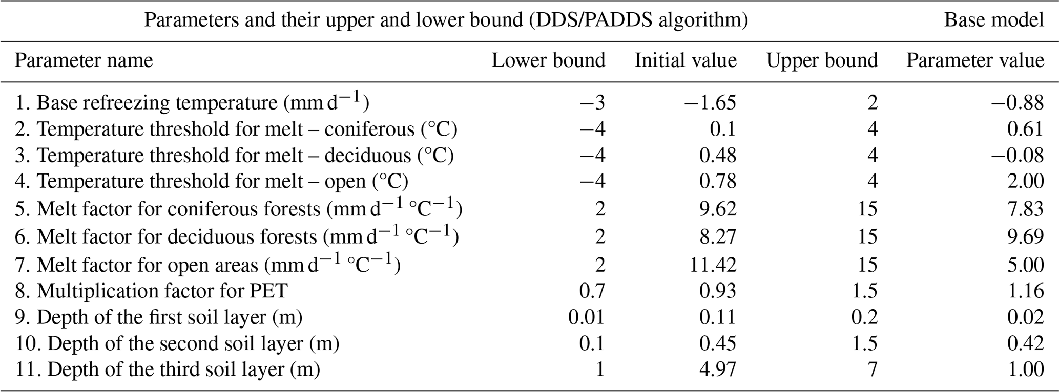
Of all parameters that are available in different modules, a subset of 11 parameters was selected for model calibration, as listed in Table 1. They include seven snow-related parameters, three parameters for soil layer thickness of the three-layer soil column and one parameter for converting potential evapotranspiration (PET) into actual evapotranspiration. The snow-related parameters affect the variation of SWE in each RHHU, while the other parameters affect runoff that is generated by the model. These parameters are selected based on sensitivity analyses done in previous studies on different watersheds (Bouda et al., 2014; Huot et al., 2019; Lucas-Picher et al., 2020).

Table 1 Lower and upper bounds of the parameters and initial parameter values of base model.

2.3 Meteorological and streamflow data

For this study, HYDROTEL is forced with spatially distributed meteorological precipitation and minimum and maximum temperature data. For precipitation, the data that are used are from MSWEP (Multi-Source Weighted-Ensemble Precipitation), which is a reanalysis product combining satellite data, gauge data and numerical weather model output. MSWEP is available globally on daily and 3 h bases from 1979 until today (http://www.gloh2o.org/mswep/, last access: 25 February 2024). The grid cell resolution of the data is 0.1°, which is about 10 km at the Equator. Overall, MSWEP offers superior performance compared to other datasets (e.g., ERA-5 Interim, ERA-5 and CHIRP) (Beck et al., 2017; Xiang et al., 2021). The ERA5-Land dataset is used for maximum and minimum air temperature. ERA5-Land has been produced by numerical integrations of the global high-resolution ECMWF land surface model with ERA5 climate reanalysis with elevation correction (Muñoz-Sabater et al., 2021) with a grid cell resolution of 0.1° (about 9 km native). The gridded data for both MSWEP precipitation data and ERA5-Land temperature data that were used in our study range from October 2000 to September 2020 and cover 45°10^′ N to 45°50^′ N and 71° W to 71°30^′ W. Observed daily streamflow data that were used for model calibration originate from the Ministère de l’Environnement, de la Lutte contre les changements climatiques, de la Faune et des Parcs station (NAD83; 45°34^′48” N, 71°23^′6^′′ W). The streamflow station is Au Saumon (030282), which is located 1.9 km upstream from the watershed outlet (see Fig. 1). The streamflow data are available on a daily basis from 1974 and onward.

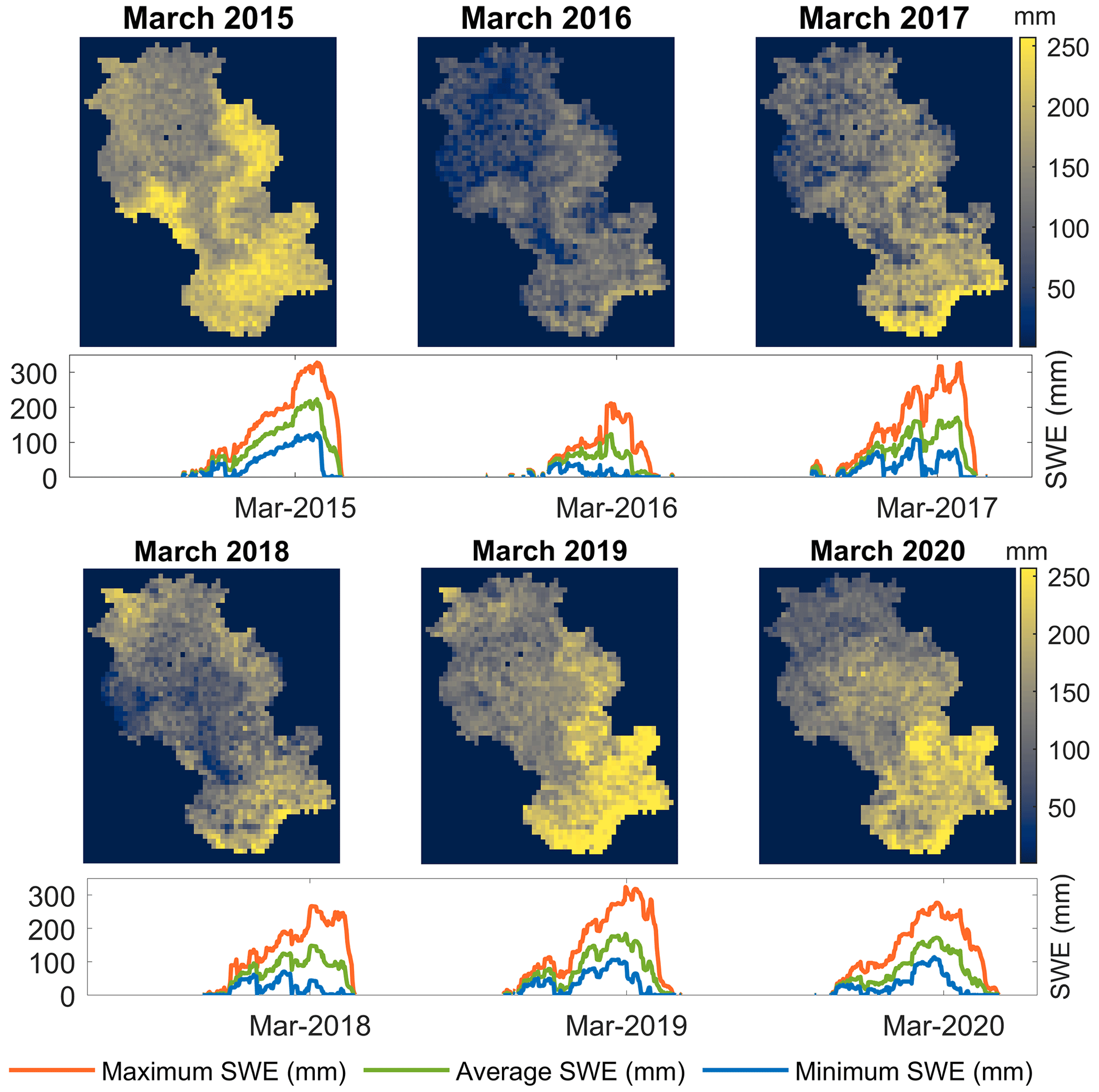
Figure 2 Spatially distributed average SWE for March, together with maximum, minimum and mean SWE for the years 2015 to 2020.

SWE data from SNODAS are used as observed data for model calibration. Figure 2 represents the spatial distribution of average SWE for the month of March for the period 2015–2020 as obtained from SNODAS, together with the temporal maximum, minimum and average of SWE across the Au Saumon watershed. It is clearly indicated in the figure that the spatial distribution varies from year to year, even when the spatially averaged values of SWE are in close agreement with each other. This is the case for the years 2017 and 2018 and for the years 2019 and 2020, where a difference of about 10 mm in average SWE in March is observed. In this study, average SWE of March is selected for the spatial calibration experiment (SPAEF calculation) as it is the month of maximum snow and maximum snow variability (transition from winter to spring, an important period when snowmelt processes are distinct). For our study, model calibration was performed for the period spanning 2014 to 2020, given that SNODAS data for the Au Saumon region are available from 2014 onwards, while model validation of streamflow was only conducted for the period ranging from 2001 to 2013.

3 Methodology

Hydrological models are typically calibrated using a single objective function, which focuses on only one aspect of the hydrological features, i.e., streamflow (Tolson and Shoemaker, 2007). As hydrological models have multiple outputs, this draws attention towards using a multi-objective approach to explore the various hydrological information that is stored in hydrological data and, thus, moving toward a multi-objective model calibration. Several studies conducted in the past suggest that optimizing two or more objective functions simultaneously may provide a better overall calibrated hydrological model (Efstratiadis and Koutsoyiannis, 2010; Adeyeri et al., 2020; Budhathoki et al., 2020). To evaluate the added value of calibration, taking into account spatial variation of the snow, different calibration experiments are performed using search algorithms: DDS (Dynamically Dimensioned Search) (Tolson and Shoemaker, 2007) for single objective functions and PADDS (Pareto Archived Dynamically Dimensioned Search) (Asadzadeh and Tolson, 2013) for multi-objective functions, with the distributed hydrological model HYDROTEL (Fortin et al., 2001) to optimize model performance. DDS is a global optimization algorithm for automatic calibration of hydrological models (Tolson and Shoemaker, 2007), which optimizes one objective function at a time without requiring algorithm parameter tuning. In contrast, PADDS is a multi-objective dynamic algorithm that uses DDS as a search engine to optimize multiple objective functions by perturbing one non-dominated solution every iteration and archiving all non-dominated solutions throughout the search. The PADDS algorithm offers multiple selection metric functions, for example, random selection, crowding distance (CD), hypervolume contribution (HVC) and convex hull contribution (CHC). To learn more about these metrics, please refer to Jahanpour et al. (2018) and Tolson and Jahanpour (2018). In this study, the HVC selection metric was chosen for the PADDS multi-objective calibration method. The effectiveness of this metric has been demonstrated in previous research (Asadzadeh and Tolson, 2013). When used with multi-objective functions the HVC measures the increase in hypervolume achieved by adding a solution to an existing set and explores the Pareto front, which represents a range of optimal trade-off solutions, by dynamically adjusting the dimensionality of the search space. Solutions with higher HVC values are prioritized to improve the coverage of the Pareto front, enhancing the overall quality of the calibration process. In this study, DDS is used when only one objective function is used at a time for calibration, i.e., the first three experiments, while PADDS is used to optimize the model with two or more objective functions simultaneously. This article focuses on utilizing the spatially distributed snow information to calibrate the model to achieve better model performance with respect to both SWE and streamflow. A total of 1000 iterations were conducted for both DDS and PADDS to optimize parameter values. The objective functions that are used during calibration are NSE (Nash–Sutcliffe efficiency) for streamflow, RMSE (root-mean-square error) for optimization of SWE over each RHHU (relatively homogeneous hydrological unit) and SPAEF (spatial efficiency metric) for spatially distributed optimization of SWE. As NSE cannot be spatialized but can only be calculated on the average SWE over the watershed, here we preferred RMSE as an objective function to calibrate SWE because it can be applied to each RHHU (spatially) and not only on the average SWE. In addition, the Kling–Gupta efficiency (KGE) is utilized for validation purposes. The Supplement presents a thorough analysis of the trade-offs between different objectives: NSE_Q and RMSE_SWE and NSE_Q and SPAEF_SWE. Readers are encouraged to refer to the Supplement for an in-depth exploration of these trade-offs and gain valuable insights into the performance of the algorithm with respect to the mentioned objectives.

The objective functions selected for this study and the optimization algorithms are now presented in the next section.

3.1 Objective functions used in the study

In this study, the NSE, RMSE and SPAEF are employed as objective functions for calibration, while the KGE is used for validation of the model. By using these three objective functions, various calibration experiments were designed to assess the strengths and weaknesses of each experiment in evaluating overall model performance.

NSE (Eq. 1) is used to evaluate the predictive skill of hydrological models. It basically compares error variance of the simulated time series, which are typically flow data, with the magnitude of the observed time series.

$$\begin{array}{}\text{(1)}& \mathrm{NSE}=\mathrm{1}-{\displaystyle \frac{{\sum }_{t=\mathrm{1}}^T{\left(Q_{\mathrm{o}}^t-Q_{\mathrm{m}}^t\right)}^{\mathrm{2}}}{{\sum }_{t=\mathrm{1}}^T{\left(Q_{\mathrm{o}}^t-{\stackrel{\mathrm{‾}}{Q}}_{\mathrm{o}}\right)}^{\mathrm{2}}}},\end{array}$$

where Q_o is observed discharge, ${\stackrel{\mathrm{‾}}{Q}}_{\mathrm{o}}$ is the mean of observed discharges and Q_m is modelled discharge.

The efficiency ranges from −∞ to 1. The value of NSE is maximized during model calibration. In this study, the NSE is calculated between the observed flow at discharge station and the simulated flow at the corresponding RHHU.

RMSE (Eq. 2) is the standard deviation of prediction errors.

$$\begin{array}{}\text{(2)}& \mathrm{RMSE}=\sqrt{\sum _t^N\sum _i^{\mathrm{RHHU}}{\displaystyle \frac{\begin{array}{l}({\text{SWE\_HYDROTEL}}_{\text{RHHU},t}\\ -{\text{SWE\_SNODAS}}_{\mathrm{RHHU},t}{)}^{\mathrm{2}}\end{array}}{N\cdot \mathrm{RHHU}}}},\end{array}$$

where t is the time step, and N is the number of time steps when HYDROTEL or SNODAS has a non-zero SWE value. SWE_HYDROTEL is the SWE computed by HYDROTEL for each RHHU and time step, and SWE_SNODAS is the average SWE of SNODAS over the RHHU for each time step. In this study, the RMSE is calculated for each of the 205 RHHUs within the Au Saumon watershed. The spatial RMSE values are calculated by comparing the SNODAS SWE and the simulated HYDROTEL SWE. Subsequently, the RMSE is minimized to enhance the model's performance.

SPAEF (Eq. 3) is a metric that is used to assess the spatial performance of a model, as opposed to NSE and RMSE, which are used to evaluate temporal model performance. SPAEF has been developed to calibrate distributed hydrological models so as to better represent the spatial variability of hydrological processes (Demirel et al., 2018; Koch et al., 2018; Demirel, 2020). In our study, SPAEF is used for assessing spatial patterns of SWE. SPAEF is calculated according to the following equation:

$$\begin{array}{}\text{(3)}& \mathrm{SPAEF}=\mathrm{1}-\sqrt{(A-\mathrm{1}{)}^{\mathrm{2}}+(B-\mathrm{1}{)}^{\mathrm{2}}+(C-\mathrm{1}{)}^{\mathrm{2}}},\end{array}$$

where

$$\begin{array}{rl}& A=\mathit{\rho }(\mathrm{obs},\mathrm{sim})\\ & B=\left({\displaystyle \frac{{\mathit{\sigma }}_{\mathrm{sim}}}{{\mathit{\mu }}_{\mathrm{sim}}}}\right)/\left({\displaystyle \frac{{\mathit{\sigma }}_{\mathrm{obs}}}{{\mathit{\mu }}_{\mathrm{obs}}}}\right)\\ & C={\displaystyle \frac{{\sum }_{j=\mathrm{1}}^{n}min\left(K_j,L_j\right)}{{\sum }_{j=\mathrm{1}}^n{K}_j}}.\end{array}$$

A is the Pearson correlation coefficient between the observed and simulated pattern; B is the fraction of the coefficient of variation representing spatial variability; and C is the histogram intersection for the histogram L of the simulated pattern and the given histogram K of the observed pattern, each containing n bins. The value of SPAEF ranges between −∞ and 1. A SPAEF value equal to 1 means that the simulated pattern perfectly matches the observed pattern, while a value of 0 means that there is no agreement between the predicted pattern and the observed pattern, which indicates that the model’s predictions are entirely inaccurate and do not align with the observed data. An advantage of SPAEF is that it equally balances three distinct individual metrics (A, B and C above) that individually would not appropriately characterize spatial patterns. For example, Koch et al. (2018) show good correlations may occur between observed and simulated patterns, while a visual interpretation of the patterns suggests this is not the case. Using a multiple-component metric, such as SPAEF, helps disentangle such inconsistencies. Koch et al. (2018) used SPAEF to calibrate the mesoscale Hydrological Model (mHM) for spatial distributions of actual evapotranspiration (AET). The study highlighted the importance of incorporating spatial observations into model calibration, since different ET patterns were obtained for similar simulated streamflow time series, depending upon the objective function that was used in the calibration process.

The SPAEF formulation is inspired by Kling–Gupta efficiency (Eq. 4) that is characterized by equally weighted components of variability, correlation and bias (Gupta et al., 2009) and is used frequently to evaluate streamflow simulations. In this study, SPAEF is used for calibrating the HYDROTEL model with respect to the spatial distribution of SWE. Given that Au Saumon is a snow-dominated watershed during winters and the maximum snow is accumulated during the month of March, it was selected for spatial calibration. While calibrating the model using SPAEF, a spatial grid is utilized. The SWE values from SNODAS are in a 60⋅58 grid for the Au Saumon watershed. For spatial calibration, the mean SWE of each grid for the month of March is taken into account. This resulted in 60⋅58 spatially distributed SWE values for each calibration year. Subsequently, the SWE simulated by HYDROTEL for the same month (March) is transformed to match the same 60⋅58 spatial distribution of SWE values. These spatial patterns, representing SWE, are then calibrated using the SPAEF

Other metrics used in this study

One other metric, KGE (Kling–Gupta efficiency), is computed for all the calibration experiments. It has been used to assess overall model performance for the various calibration scenarios that were investigated in this study.

$$\begin{array}{}\text{(4)}& \mathrm{KGE}=\mathrm{1}-\sqrt{(R-\mathrm{1}{)}^{\mathrm{2}}+{\left({\displaystyle \frac{{\mathit{\sigma }}_{\mathrm{sim}}}{{\mathit{\sigma }}_{\mathrm{obs}}}}-\mathrm{1}\right)}^{\mathrm{2}}+{\left({\displaystyle \frac{{\mathit{\mu }}_{\mathrm{sim}}}{{\mathit{\mu }}_{\mathrm{obs}}}}-\mathrm{1}\right)}^{\mathrm{2}}}\end{array}$$

KGE is calculated as in Eq. (4), where R is the Pearson correlation coefficient between observed and simulated streamflow time series, σ_obs is the standard deviation in observations, σ_sim the standard deviation in simulations, µ_sim is the simulated mean streamflow, and µ_obs is the observed mean streamflow.

3.2 Proposed calibration approach

Seven different experiments were set up, with each experiment being characterized by a unique combination of objective functions and calibration strategy (see Table 2). All calibration experiments were performed on the base model, which is defined as a model that was run with some random value without prior knowledge based upon previous studies done on similar catchments. Initial parameter values of HYDROTEL (the base model) are presented in Table 1. HYDROTEL was calibrated over a 6-year period, from October 2014 to September 2020. Prior to model calibration, a 2-year warm-up period was set up to avoid any effects of initial model conditions on its results during calibration. Validation extends from 2001 to 2014. In addition to data availability, one important aspect for choosing the calibration period was to include winter seasons that were characterized by low, average and high SWE values. Winters in 2019 and 2020 especially were considered high- and low-winter seasons, with corresponding basin-averaged SNODAS SWE values of 156.05 and 86.26 mm, respectively, at the onset of the spring melt season. The number of iterations also was fixed (1000) for each calibration for comparison. Lower and upper bounds of the parameters that were used in all calibration experiments are presented in Table 1.

Table 2 Calibration experiments with their corresponding objective functions that were used.

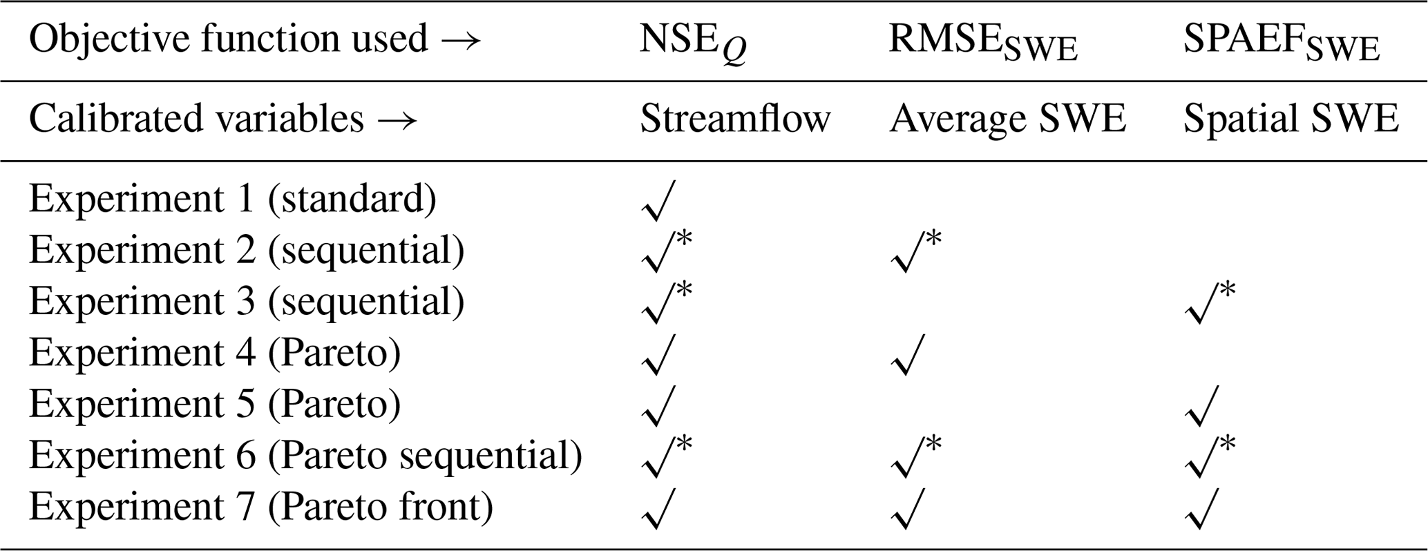
${\surd }^{*}$ Streamflow is calibrated with NSE sequentially after optimizing SWE with either RMSE or SPAEF.

Table 2 presents all calibration experiments that were performed in this research. The first calibration experiment, hereafter denoted as the “standard” experiment, refers to the traditional calibration process that was based upon maximizing NSE_Q, which was calculated with simulated and observed streamflow time series. In this experiment, all 11 parameters that are listed in Table 1 are optimized using the DDS algorithm. Experiments 2 and 3 consist of adding SWE information during the calibration procedure. This is done by sequentially calibrating HYDROTEL, first by adjusting the snow-related parameters (parameters 1 to 7; see Table 1) to minimize RMSE_SWE (Experiment 2) or to maximize SPAEF_SWE (Experiment 3) using DDS, after which the runoff-related parameters (8 to 11) are adjusted with NSE_Q for streamflow, again using DDS, while the snow parameters are left unchanged. Experiments 4 and 5 consist of adding both streamflow and SWE information once with average information of SWE (Experiment 4) and once with spatial information of SWE (Experiment 5) in the calibration procedure. This was achieved by maximizing NSE_Q and minimizing RMSE_SWE at once (Experiment 4) and by maximizing both NSE_Q and SPAEF_SWE (Experiment 5) using PADDS. Experiment 6 consists of adding both spatial and average SWE information in the calibration procedure. This is done by sequentially calibrating HYDROTEL, first by adjusting the snow-related parameters to minimize RMSE_SWE and maximize SPAEF_SWE together using PADDS, after which NSE_Q for streamflow was maximized while the snow parameters are left unaltered. In Experiment 7, all 11 parameters are optimized while maximizing NSE_Q for streamflow and SPAEF_SWE for spatial information of SWE and minimizing RMSE_SWE for average information of snow.

4 Results

Values of the objective functions for each of the calibration and validation experiments are summarized in Table 3. The values of objective functions NSE_Q, RMSE_SWE and KGE_Q corresponding to the base model are 0.630, 48.83 mm and 0.806, respectively. Using the same base model would be helpful in evaluating whether the calibration performed is adequate for the model’s performance. When the model is calibrated with respect to SWE (for both average and spatial calibration), parameters from 1 to 7 are calibrated; when calibrating with respect to streamflow, all the 11 parameters are considered.

Table 3 All calibration experiments with their corresponding parameters and objective function values. Bold values indicate when the parameters reach the boundary values, and bold italic values indicate the calibration and validation results for all the metrics.

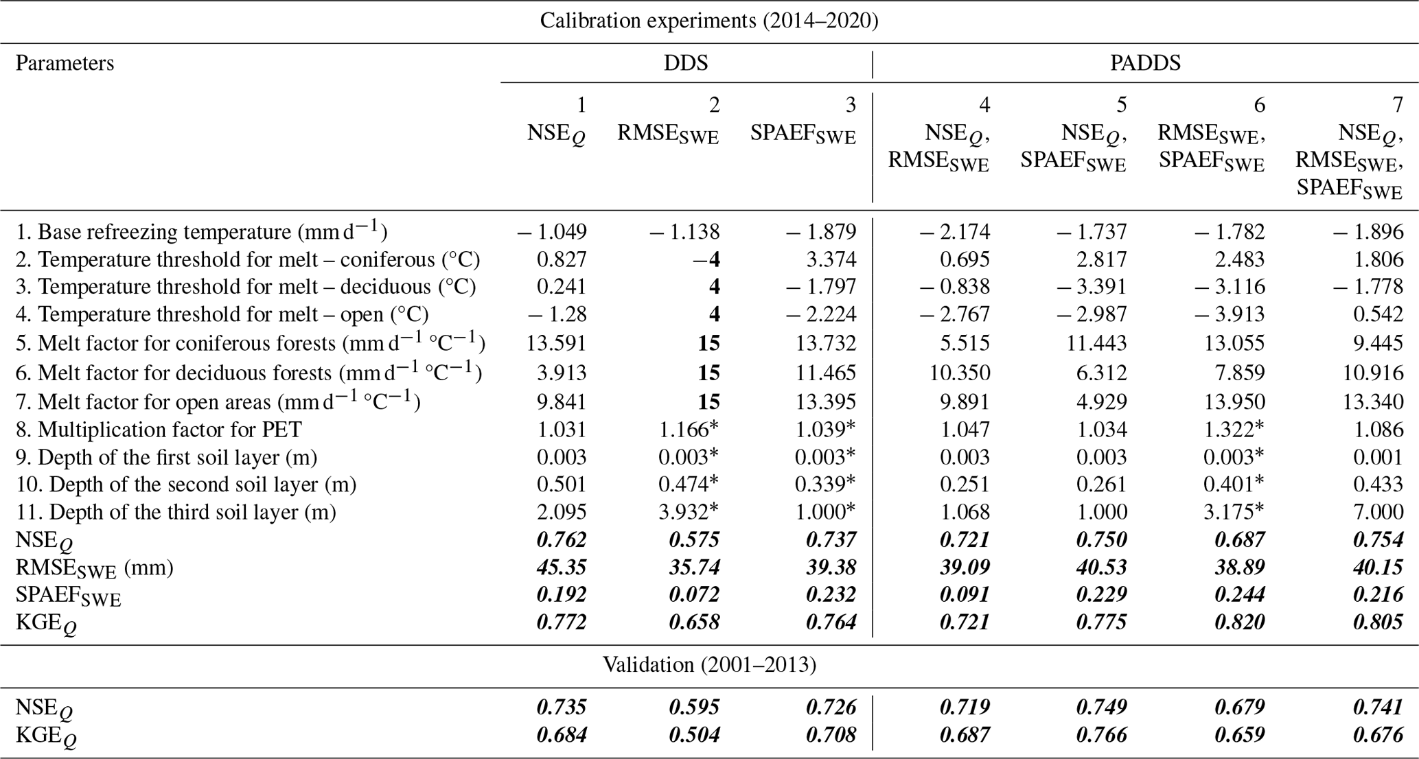
^* These values are obtained after sequential calibration with NSE.

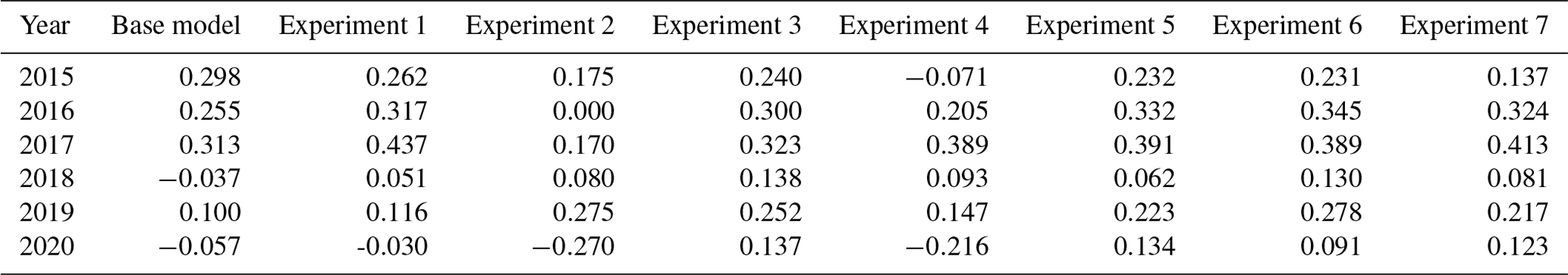
Table 4 SPAEF_SWE values for each year from each experiment with the best value of 0.437 (Experiment 1 – 2017) and the worst value of −0.270 (Experiment 2 – 2020).

The first experiment is standard practice for calibrating hydrological models. The simulated streamflow in the standard experiment generally follows the same temporal pattern for all calibrated years as that of the observed streamflow, but the model has some difficulties in capturing peak streamflow (Fig. 3). More specifically, the model generated more streamflow during winter 2020 (January to April 2020). The observed discrepancy between the simulated and observed streamflow during different seasons indicates potential inadequacy of the model in effectively representing the complex hydrological processes occurring during various seasons, including snowmelt and spring runoff. For the study period, rain-on-snow events are identified based upon the occurrence of precipitation during winter months, along with a decrease in snow depth, coupled with a maximum temperature that exceeds 0°C. Within this experiment, the model demonstrates the capability to identify melting patterns during rain-on-snow events. However, it exhibits limitations in accurately capturing both high and low peaks of SWE (Fig. 4). As rain-on-snow events during winter produce runoff, the model tends to interpret these as streamflow. Simulated streamflow is relatively similar to the observed streamflow after the events. For the calibration period, values of 0.762 and 0.772 are obtained in this experiment for NSE_Q and KGE_Q, respectively. When compared with the base model, the NSE_Q value is improved (from 0.630 to 0.762), which is expected given that NSE_Q is the objective function. The KGE_Q value slightly declined from 0.806 to 0.772, suggesting a slight decrease in hydrological model simulation accuracy, indicating a potential mismatch between observed and simulated hydrographs. The model is validated for the 2001–2013 period, and the NSE_Q value that was obtained is 0.735, thereby indicating good agreement between observed and simulated streamflow values. The KGE_Q value that was obtained is 0.684, which suggests moderate agreement during the validation period. The spatially averaged RMSE_SWE value of SWE for the watershed with respect to SNODAS-SWE is 45.35 mm. Figure 4 indicates that HYDROTEL tends to overestimate SWE compared to SNODAS, except for year 2020. During this year, the model generates notably higher streamflow in winter (Fig. 3) compared to the observed data. Either insufficient winter precipitation in the hydrological model or inaccurate temperature data for the year 2020 could be contributing factors to this issue. Upon comparing precipitation data for 2020 with precipitation that was obtained from meteorological stations, discrepancies were observed in the MSWEP precipitation data, particularly some missing peaks during the winter season. These discrepancies in the precipitation data could potentially contribute to the unusual output that was observed in the study. Through the comparative analysis of SWE data that were collected from the Milan (elevation: 496 m) and Bury (elevation: 340 m) stations, it suggests that the calibrated model exhibits a tendency to closely correspond with the values that were obtained from Milan, a station that was characterized by a higher elevation. This response suggests the substantial influence of the elevation factor on the model simulations. SPAEF is computed for SWE for the month of March for each year of the calibration period and varies from −0.030 for 2020 to 0.437 for 2017 (Table 4), indicating that the success at simulating the spatial SWE patterns by HYDROTEL is highly variable from year to year.

Figure 3 Comparison of observed streamflow with simulated streamflow for Experiment 1.

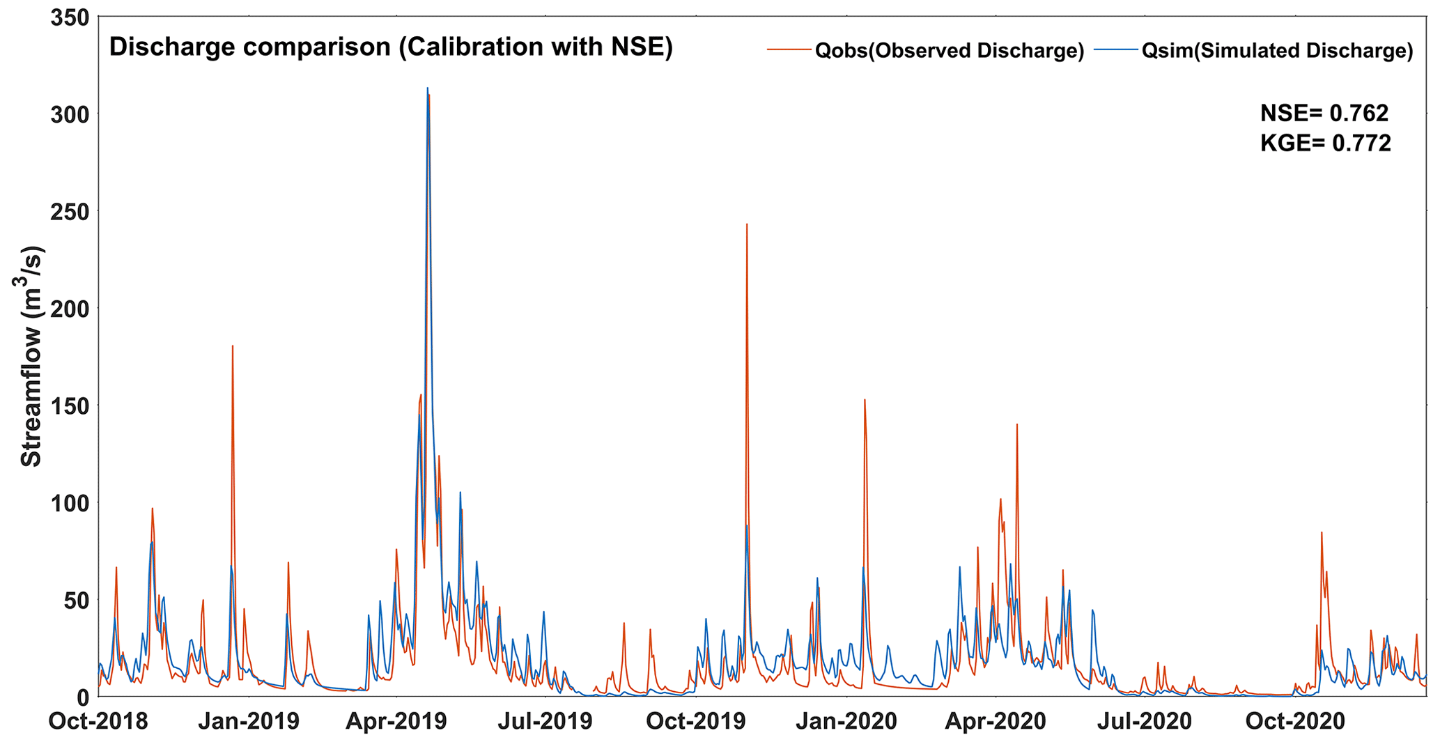
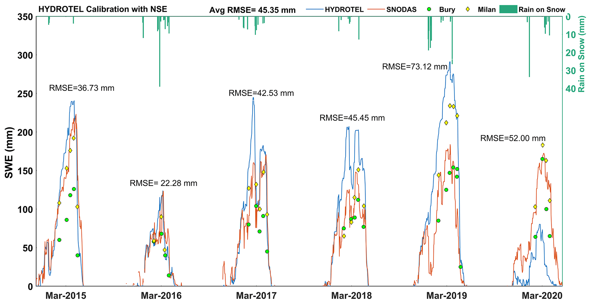
Figure 4 Comparison of SNODAS SWE with simulated SWE for Experiment 1 along with station data.

In Experiment 2, all snow-related parameters are first calibrated using RMSE_SWE with spatially averaged (considering the SWE values for each RHHUs for whole calibration period then averaging), modelled and SNODAS SWE followed by calibration of the remaining parameters with NSE_Q applied to streamflow. The average RMSE_SWE value after calibration is 35.74 mm, which is considerably improved compared with the standard calibration experiment. Indeed, Fig. 5 effectively shows that simulated SWE more closely matches SNODAS SWE compared to the standard experiment. Note that for both experiments, HYDROTEL significantly underestimates snow accumulation for winter 2020. The cause for this discrepancy remains consistent with the previously discussed reasons. NSE_Q for streamflow after sequential calibration is 0.575, and the KGE_Q value is 0.658, which are considerably lower than corresponding values for the standard experiment. The model was thus able to improve simulated basin average SWE but at the expense of a deterioration of the simulated streamflow. During rain-on-snow events in winter, the model is able to produce the peaks of SWE, but it is unable to capture accurately the associated melting patterns. Moreover, spatial distribution values of SWE varied from −0.270 (for March 2020) to 0.275 (for March 2019) (Table 4). The average SPAEF_SWE value is much lower compared to values obtained with the standard experiment. in other words, spatial heterogeneity of the snowpack deteriorates when calibration is performed with the average SWE value.

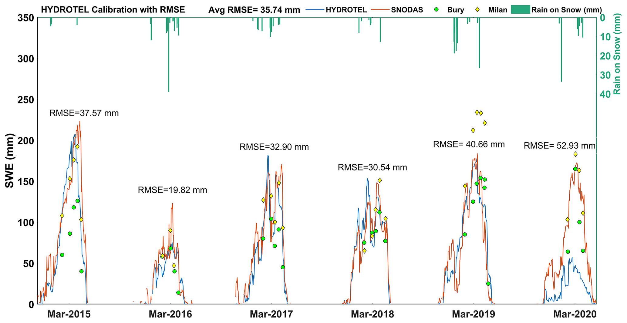
Figure 5 Comparison of SNODAS SWE with simulated SWE for Experiment 2 along with station data.

Instead of trying to preserve the best temporal dynamics of basin-averaged SWE, Experiment 3 attempts to maintain its spatial distribution at the end of the snow-accumulation season using SNODAS-SWE. This is accomplished by incorporating SPAEF_SWE as the objective function for SWE for calibrating snow-related parameters, followed by NSE_Q for streamflow to adjust the remaining parameters. Unsurprisingly, the March SPAEF_SWE value averaged over years 2015–2020 increased to 0.232, when compared to 0.192 and 0.072 for Experiments 1 and 2, respectively (Table 3). Figure 6 depicts the relationship between the spatial distribution of SNODAS and HYDROTEL and the corresponding SPAEF_SWE value. The results indicate that a greater spatial difference between SNODAS and HYDROTEL leads to a negative SPAEF_SWE value. Conversely, when the spatial distribution of both datasets is similar, SPAEF_SWE approaches 1. The figure displays the maximum, 0.437 (year 2017 – Experiment 1), and minimum, −0.270 (year 2020 – Experiment 2), values of SPAEF_SWE that were obtained during the calibration experiment.

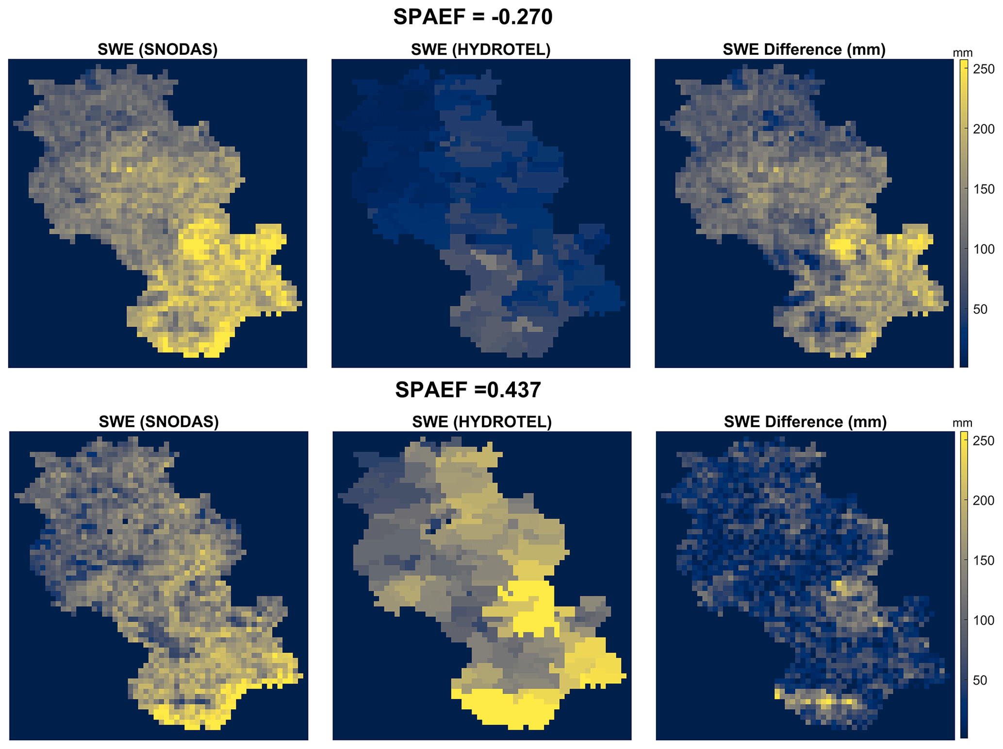
Figure 6 Spatially distributed SWE values of SNODAS and HYDROTEL, along with corresponding SWE differences for minimum (−0.270; Experiment 2, year 2020) and maximum (0.437; Experiment 1, year 2017) SPAEF_SWE values for Au Saumon watershed.

Overall, calibrating HYDROTEL using SPAEF_SWE helped preserve SWE spatial heterogeneity that was simulated by the model. Also, year-to year variability in SPAEF_SWE is reduced, as SPAEF_SWE varied from 0.137 (Mar 2020) to 0.323 (March 2017). A year-to-year comparison of spatial SWE reveals that calibrating the model with SPAEF_SWE degraded SWE distribution in some years, e.g., 0.300 (March 2016) and 0.240 (March 2015). This means that spatial integrity of the SWE value is occasionally compromised using the calibration strategy. A detrimental effect of calibrating the model with SPAEF_SWE is that the average SWE value is overestimated by the model as compared to observed average value (Fig. 7). Correspondingly, the average RMSE_SWE is 39.38 mm, which is higher than the value that is obtained when the model is calibrated using RMSE_SWE as the objective function. The sequential calibration with NSE_Q yields a value of 0.737. The KGE_Q value is 0.764, which is better than what is achieved in Experiment 2. This suggests that using spatial distribution to calibrate snow parameters apparently provides better results for streamflow than using average SWE value to calibrate snow parameters. Interestingly, both Experiments 1 and 3 overestimated spatially averaged SWE, but the sequential calibration strategy provided a good match between simulated versus observed flows, given that NSE_Q and KGE_Q values for Experiments 3 and 1 are comparable. From an experimental perspective, it is worth noting that in Experiment 3, the spatial distribution of SWE, i.e., the SPAEF_SWE value, exhibits better improvement when compared to the standard practice. Although the temporal dynamics of spatially averaged SWE are well preserved in Experiment 2, the flow-related model parameters could not be properly calibrated to obtain a good fit between observed and simulated flows. Perhaps this is due to the spatial invariance of these parameters, to the sequential modelling strategy or to both. In order to investigate the latter, experiments were performed in which NSE_Q, RMSE_SWE or SPAEF_SWE is simultaneously optimized with multi-objective calibrations (Experiments 4 to 7).

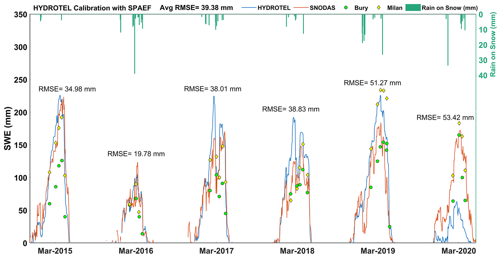
Figure 7 Comparison of SNODAS SWE with simulated SWE for Experiment 3 along with station data.

In Experiment 4, NSE_Q for streamflow and RMSE_SWE for SWE are optimized together using PADDS. The maximum value of NSE_Q is 0.721, while RMSE_SWE is 39.09 mm, which shows improvement compared to the standard experiment (Experiment 1) in terms of RMSE_SWE. Upon comparison with the sequentially calibrated experiment (Experiment 2), an improvement was observed in the NSE_Q and SPAEF_SWE values, coupled with a decrease in RMSE_SWE. Surprisingly, the comparison between Experiments 3 and 4 suggests that sequential calibration of the hydrological model using SPAEF_SWE results in better model performance in terms of NSE_Q, SPAEF_SWE and KGE_Q, in contrast to multi-objective calibration with NSE_Q and RMSE_SWE. SPAEF_SWE of SWE varied from −0.216 (for March 2020) to 0.389 (for March 2017), with an average 0.091 for all calibrated years, which is higher than the value that was obtained using RMSE_SWE and NSE_Q in a sequential calibration strategy (0.072). In other words, opting for a simultaneous RMSE_SWE–NSE_Q calibration improved the spatial SWE distribution compared to a sequential calibration strategy. The value remains below that obtained in Experiment 3 (0.232).

In Experiment 5, NSE_Q is used to optimize streamflow and SPAEF_SWE for spatial SWE together. The optimized solution yields NSE_Q of 0.750 and a KGE_Q of 0.775. Spatial distribution of SWE varied from 0.062 (for March 2018) to 0.391 (for March 2017). The average SPAEF_SWE value that was obtained for all calibrated years is 0.229. When compared with standard calibration (Experiment 1), the spatial distribution of SWE is improved (from 0.192 to 0.229), together with RMSE_SWE (from 45.35 to 40.53 mm), while NSE_Q of Experiment 5 is comparable with standard calibration with an improved KGE_Q value. Upon comparing Experiments 5 and 3, where SPAEF_SWE is calibrated followed sequentially by NSE_Q, a slight improvement in NSE_Q is noted. Yet, SPAEF_SWE and RMSE_SWE appear to be compromised. Here, sequential calibration using SPAEF_SWE results in superior performance for RMSE_SWE and SPAEF_SWE, whereas multi-objective calibration jointly yields a better performance measure for NSE_Q. Comparing the results to Experiment 4, where NSE_Q is calibrated with RMSE_SWE, it is observed that NSE_Q, KGE_Q and SPAEF_SWE are improved in Experiment 5, while RMSE_SWE results are comparable. This again suggests that using SPAEF_SWE to calibrate spatially distributed SWE is more advantageous than using RMSE_SWE to calibrate spatially averaged SWE when employing multi-objective functions with NSE_Q.

In Experiment 6, both RMSE_SWE for spatially averaged SWE and SPAEF_SWE for spatial distributed SWE are first optimized simultaneously using PADDS to calibrate HYDROTEL’s snow-related parameters, followed by maximizing NSE_Q for streamflow to calibrate the remaining flow-related parameters. After calibration, the best value for RMSE_SWE is 38.89 mm, while SPAEF_SWE values ranged from 0.091 (for March 2020) to 0.389 (for March 2017), with an average value of 0.244. Sequential calibration with NSE_Q provided a NSE_Q value of 0.687 for streamflow and a KGE_Q value of 0.820. In comparison to Experiments 4 and 5, NSE_Q has decreased substantially, while the KGE_Q value has increased substantially. This suggests that model performance has improved in terms of capturing the overall pattern of the observed data, although the accuracy in fitting individual data points may have declined slightly. In Experiment 6, a significant improvement is noted for SPAEF_SWE, with a slight decrease in RMSE_SWE compared to Experiment 4. This suggests that by sequentially calibrating both SPAEF_SWE and RMSE_SWE followed by NSE_Q, the model is able to capture the spatial distribution of both SWE and streamflow. Yet, it should be noted that the model’s fitness to individual data points might not be captured accurately. In Experiment 6, slight improvement in SPAEF_SWE was noted, with a slight decrease in RMSE_SWE, but a significant reduction in NSE_Q as compared to Experiment 5. This implies that calibrating SPAEF_SWE and NSE_Q together is a better approach than sequential calibration of SPAEF_SWE and RMSE_SWE, followed by NSE_Q under the considered model setting.

As the last step in calibration trial, all objective functions were calibrated together using the PADDS algorithm. NSE_Q after optimization is 0.754, KGE_Q is 0.805 and RMSE_SWE is 40.15 mm. Spatial distribution of SWE varied from 0.081 (for March 2018) to 0.413 (for March 2017). The average SPAEF_SWE value for all calibrated years is 0.216. When compared to the standard experiment, Experiment 7 outperforms in terms of RMSE_SWE, SPAEF_SWE and KGE_Q, while NSE_Q remains comparable in both cases. Among other experiments, Experiment 7 shows better performance when compared to Experiments 2 and 4, while results from Experiments 3 and 5 are comparable to Experiment 7. By comparing Experiment 6, where NSE_Q is sequentially calibrated with RMSE_SWE and SPAEF_SWE, and Experiment 7, where all three functions are calibrated together, we conclude that calibrating together provides better results for NSE_Q and comparable results for other objective functions.

In comparing all calibration strategies during validation, NSE_Q values for the experiments could be ordered: 5, 7, 1, 3, 4, 6 and 2. KGE values > 0.75 are generally considered to be indicative of good model performance, as noted in previous studies (Towner et al., 2019). Upon analyzing the results in calibration experiments, most are found to have KGE values greater than 0.75 for the calibration period; the exceptions are the second (calibration with RMSE_SWE and sequential NSE_Q) and fourth (calibration with RMSE_SWE and NSE_Q simultaneously) experiments. This suggests that calibration in these experiments is satisfactory, and the model is expected to perform well. The validation results from the years 2001–2013 were analyzed for the best model performance with respect to KGE_Q. Experiment 5 had the highest KGE_Q, indicating the best model performance. Experiment 3 followed closely behind, while Experiments 1, 4 and 7 produced nearly identical results. In contrast, Experiments 2 and 6 had poor performance in terms of KGE_Q. A noticeable feature of SPAEF_SWE is the amount of time that is required for calibration, together with the number of iterations to reach the best value. In this study, iterations were set at the same number to maintain comparable scenarios, while the duration of spatial calibration was twice as long as the remaining experiments.

5 Discussion

Analysis of parameter variations following calibration revealed consistent values for the base refreezing temperature, the PET parameter, and depth of the first two soil layers across multiple calibrations. Yet, variation was observed in the temperature thresholds for melt, melt factor, and thickness of the third soil layer among experiments, particularly for Experiment 2. In the initial phase of calibration experiments, several trial and error runs were conducted to determine parameter boundaries, while simultaneously reviewing relevant literature, which enhanced understanding and accuracy through comprehensive parameter exploration. Experiment 2, which used RMSE_SWE and NSE_Q sequentially, consistently reached the parameter bounds for temperature thresholds and melt factors. Depending upon the land use, temperature threshold values also show opposite values, i.e., −4 °C for conifers versus 4 °C for deciduous and open areas. This means that there are areas with a lot of snow and others with very little snow in the watershed based on land use, which does not represent the accurate spatial distribution of snow for this watershed. The watershed exhibits a significant predominance of coniferous vegetation, leading to a lower temperature threshold in Experiment 2 compared to the other experiments. Experiment 1 overestimates SWE compared to SNODAS. By decreasing the temperature at which melting begins for a large portion of the watershed, Experiment 2 decreases the overall quantity of snow to levels closer to SNODAS values. Yet, the spatial distribution of snow is not respected. Therefore, it is not recommended that parameters using RMSE_SWE and NSE_Q be calibrated sequentially.

As the research objective, this study evaluated the practicality of using raw SNODAS data for hydrological model calibration. A number of research studies have been done previously using bias-corrected SNODAS and raw SNODAS information. King et al. (2020) revealed a significant enhancement in area melt estimates during the spring melt when utilizing bias-corrected SNODAS-SWE data compared to raw SNODAS estimates, which exhibited unrealistic melt volumes. The study's comparisons with in situ SWE measurements demonstrated that nonlinear bias correction techniques notably improve the accuracy of SNODAS SWE estimates. Zahmatkesh et al. (2019) showcased that bias-correcting SNODAS SWE significantly enhanced the accuracy of lumped models, contrasting with raw SNODAS SWE, which resulted in overestimated streamflow and peak flow values. A significant limitation in bias-correcting SNODAS data lies in the absence of substantial data (Zahmatkesh et al., 2019). Given its specific focus, bias correction of the SNODAS data was not within the scope of the study. As a result, raw SNODAS data were employed for analysis of SWE, and both RMSE and SPAEF were utilized as objective functions to calibrate SWE in the model. In Experiment 2, RMSE_SWE can drive the parameters to extreme values, given that it treats all data points equally irrespective of their location in the distribution. If there are extreme values in the observed data, the model can be calibrated to fit those values, even if they do not represent the overall distribution. This can lead to poor model performance when applied to new data or different conditions. The sensitivity of RMSE to outliers is a common concern while using it in calibration. Outliers can significantly impact RMSE calculations, and their likelihood of occurrence aligns with the normal distribution that underlies RMSE (Chai and Draxler, 2014). When model biases are pronounced, it may be necessary to address these systematic errors before calculating RMSE. However, the bias insensitivity of SPAEF offers a valuable solution to this challenge (Koch et al., 2018). SPAEF mitigates the impact of uncertainties in observations, providing a more robust and stable approach to model calibration and evaluation. In such situations, SPAEF may be a more reasonable option to achieve good calibration of SWE when bias correction of data is not feasible.

Our study focuses on incorporating snow spatial information into hydrological model calibration. A novel spatial efficiency metric called SPAEF was utilized in conjunction with other objective functions, i.e., RMSE and NSE. NSE was employed as an objective function for streamflow. It enables direct evaluation of model performance against the inherent benchmark of NSE =0, which corresponds to the mean flow. Alongside other metrics, KGE was computed for both calibration and validation. Knoben et al. (2019) suggested that KGE values falling within the range of $-\mathrm{0.41}<\mathrm{KGE}\mathrm{\le }\mathrm{1}$ can be considered reasonable for hydrological modelling. This indicated a satisfactory representation of the observed data, taking into account the limitations and uncertainties that were associated with the model and data. Consequently, KGE was utilized as a performance metric to compare validation results, with Table 3 summarizing the corresponding parameter values for each calibration experiment. Based upon the comparison of validation results using KGE_Q, it is evident that incorporating spatial calibration with SPAEF_SWE in conjunction with NSE_Q (in both simultaneous and sequential calibrations) yields better outcomes compared to utilizing RMSE_SWE as one of the objective functions or using NSE_Q as only objective function.

Looking at first three experiments, it can be inferred that the sequential calibration of NSE following the calibration of spatially distributed SWE with SPAEF_SWE yields outcomes that exhibit better acceptability as the overall model performance is enhanced. The reason for this is that calibrating SWE captures the spatial variability of the snowpack, which is a crucial factor in hydrological processes. Calibrating NSE_Q subsequently ensures that the model can capture temporal variation of the flow. Therefore, the sequential calibration approach leads to better results that are acceptable in terms of overall model performance. When comparing results of calibration with RMSE_SWE and calibration with SPAEF_SWE, followed by sequential NSE_Q calibration, it is evident that SPAEF_SWE yields better results than RMSE_SWE. The distribution of snow is not uniform everywhere; therefore, spatially distributed SWE calibration captures the heterogeneity of the snow distribution within the basin, whereas spatially averaged snow calibration assumes that snow is uniformly distributed throughout the basin, which is not always the case in mountainous terrain where snow can accumulate in complex patterns. Thus, spatially distributed SWE calibration provides a more accurate estimate of the actual snow distribution in the basin, which leads to better model performance in predicting streamflow.

In a comparative analysis of hydrological model calibration procedures, Tuo et al. (2018) examined the effectiveness of different calibration approaches. Their study focused upon the multi-objective calibration method, specifically incorporating the optimization of sub-basin average snow water equivalent (SWE) and streamflow. The results demonstrated that this multi-objective approach outperformed single-objective procedures in accurately simulating snow dynamics, which aligns with our study. Building upon these findings, our study extended the calibration process by further incorporating both spatially averaged and spatially distributed data for SWE. Notably, our results highlighted the superiority of calibrating the model using spatially distributed information rather than relying solely upon average information. Considering the spatial distribution of SWE data leads to improved model performance and more accurate simulations.

Focusing upon multi-objective calibrations, Experiments 4 and 5 also back up the aforementioned argument that using SPAEF_SWE with NSE_Q yields better results than using RMSE_SWE with NSE_Q. Based upon the comparisons made in Experiments 2 vs. 4, 3 vs. 5 and 6 vs. 7, it is evident that calibrating the objective functions simultaneously yields superior model performance compared to the sequential calibration of the objectives. Specifically, Experiments 4, 5 and 7, which employ the simultaneous calibration of objective functions that were considered, exhibit improved model performance when compared to Experiments 2, 3 and 6, which adopt a sequential calibration approach. The study that was conducted by Finger et al. (2015) showcased the benefits of calibrating a hydrological model using multiple datasets, thereby leading to improved estimation of runoff contribution. This finding is consistent with the current study, which highlights calibrating both SWE and streamflow as yielding superior results. From our study, it can be concluded that simultaneous calibration of objective functions is a superior approach to sequential calibration, given that sequential calibration can lead to overfitting of the model to the specific objective function being calibrated. In turn, this can result in poor model performance when evaluating other objective functions. Furthermore, sequential calibration may result in a trade-off between objective functions, which may not be optimal for overall model performance. When all objective functions are calibrated simultaneously, it allows for a more balanced calibration and can provide better overall model performance. It also helps avoid overfitting to any single objective function and provides a more comprehensive understanding of the model’s behaviour.

For this study, March was selected for SPAEF calibration as it is the month with the highest SWE. Our objective was to leverage the maximum SWE information available during this period. However, we recognize that March, despite having the highest SWE, also overlaps with the snowmelt period, which could potentially influence the calibration of our analysis. We performed additional analyses using data from January and February, and the results demonstrated that SPAEF performs well with data from both these months. We believe that further research is necessary, with different watersheds and periods used to compute SPAEF, to more accurately understand SPAEF's performance during the onset of snow accumulation and the snowmelt period. The detailed results of these additional calibrations can be found in the Supplement, providing a comprehensive view of the model's performance.

6 Conclusions

Hydrological models are subject to continuous development, becoming more sophisticated over time, as a result of advancements in computational resources and a better understanding of hydrological processes. These models are not merely tools for estimating runoff; rather, they encompass simulation of complex processes that involve state variables contributing to the generation of runoff. The satellite input data, which are used to drive these models, are available at high temporal (ranging from daily to hourly) and spatial resolutions (up to a kilometre scale). Integration of comprehensive spatial data that are acquired from remote sensing platforms offers tremendous opportunities for further advancements in hydrological modelling.

This article analyzes different calibration experiments of the HYDROTEL distributed hydrological model for the Au Saumon watershed. HYDROTEL includes modules that permit high-resolution discretization of the basin, river streams, lake inflow, river flow and gridded observed meteorological data, making it a suitable model for the calibration experiment. The key aspect of this calibration experiment is the incorporation of the spatial efficiency metric SPAEF as an objective function. The study explored this newly developed spatial distribution metric in the calibration and validation of distributed hydrological models and compared results with previously used calibration strategies. SPAEF has been used previously with evapotranspiration in various studies, but this study introduces SPAEF with SWE for the first time. The comparison of different calibration strategies on the Au Saumon watershed highlights these important findings.

• Calibrating only streamflow is not ideal for distributed hydrological model. It is recommended that snow variables such as snow water equivalent (SWE) also be calibrated, especially in areas where snow accumulation can be spatially heterogeneous.

• Sequential calibration of objective functions (e.g., calibrating using NSE after calibrating with SPAEF) may not always result in better model performance compared to calibrating all objective functions simultaneously, especially when considering multiple objective functions. Sequential calibration of objective functions is not recommended, as it may result in sub-optimal model performance.

• Spatially distributed SWE calibration is preferred over spatially averaged calibration, given that the former captures heterogeneity of snow distribution in different land covers and provides more accurate estimates of SWE across the basin.

• Raw SNODAS data have the potential for enhancing the model’s accuracy and reliability by incorporating the spatial variability of snow distribution.

The present experiments demonstrate that although researchers tend to focus upon obtaining decent model output by optimizing a single objective function, this approach may not provide entirely reliable results. Therefore, using multiple objective functions to optimize different processes simultaneously can lead to better results. In this study, the importance of incorporating the spatial calibration metric SPAEF is highlighted. Spatial calibration of snow variables provides better results when compared to averaging the variables. To further understand the spatial metric, it is necessary to investigate spatial variability and SPAEF by applying and comparing it to other catchments or models. Calibrating a distributed model and increasing its spatial predictability requires more than just an appropriate spatial performance indicator. It necessitates the use of a flexible model structure and parameterization in conjunction with other metrics to enable simulated patterns to be modified meaningfully. Achieving this requires reliable geographic measurements at an appropriate scale, thorough assessment of catchment morphology, and high-quality forcing data.

Based upon our findings, it is evident that spatial calibration of a distributed hydrological model, HYDROTEL, yields satisfactory results and enhances its robustness and coherence with other hydrological processes. Our study aims to encourage the modelling community to reconsider their methodologies by focusing upon relevant metrics that emphasize spatial patterns characterizing hydrological processes during calibration or validation studies. The upcoming Terrestrial Snow Mass Mission (TSMM) satellite mission (low-cost, low-mass, spaceborne Ku-band synthetic aperture radar (SAR) system that is being developed by the Canadian Space Agency; Derksen et al., 2021) seeks to offer high-resolution and spatially distributed information on SWE. Consequently, to optimize hydrological model performance, calibration procedures that account for both conventional streamflow and spatial SWE should be considered.

The study, while conducted for a single watershed, contributes to our understanding of SPAEF’s performance in hydrological modelling of snow-dominated watershed. However, it also reveals the need for further research. The utilization of different precipitation and temperature datasets as input data can significantly impact the performance of hydrological models. Variations in these datasets, which may arise from differences in data collection methods, spatial resolution and temporal coverage, can affect the reliability and accuracy of hydrological predictions. The distinct characteristics of each watershed used, including size, slope, altitude and land, can have a substantial impact on the snow accumulation and melt processes. Therefore, it is essential to broaden this research to include different watersheds and various input data to validate and generalize our findings. Moreover, snow accumulation and melt do not occur uniformly throughout the year but happen in distinct periods. Our study focused on the month of maximum SWE (March), but the accumulation and melt periods of the snow season are both important. Future studies should consider different snow periods to gain a better understanding of SPAEF’s performance. Finally, the choice of input data (precipitation and temperature) can have an impact on the spatial distribution of snow variables simulated by the model.