Synthesis of historical reservoir operations from 1980 to 2020 for the evaluation of reservoir representation in large-scale hydrologic models

All the major river systems in the contiguous United States (CONUS) (and many in the world) are impacted by dams, yet reservoir operations remain difficult to quantify and model due to a lack of data. Reservoir operation data are often inaccessible or distributed across many local operating agencies, making the acquisition and processing of data records quite time-consuming. As a result, large-scale models often rely on simple parameterizations for assumed reservoir operations and have a very limited ability to evaluate how well these approaches match actual historical operations. Here, we use the first national dataset of historical reservoir operations in the CONUS domain, ResOpsUS, to analyze reservoir storage trends and operations in more than 600 major reservoirs across the US. Our results show clear regional differences in reservoir operations. In the eastern US, which is dominated by flood control storage, we see storage peaks in the winter months with sharper decreases in the operational range (i.e., the difference between monthly maximum and minimum storage) in the summer. In the more arid western US where storage is predominantly for irrigation, we find that storage peaks during the spring and summer with increases in the operational range during the summer months. The Lower Colorado region is an outlier because its seasonal storage dynamics more closely mirrored those of flood control basins, yet the region is classified as arid, and most reservoirs have irrigation uses. Consistent with previous studies, we show that average annual reservoir storage has decreased over the past 40 years, although our analyses show a much smaller decrease than previous work. The reservoir operation characterizations presented here can be used directly for development or evaluation of reservoir operations and their derived parameters in large-scale models. We also evaluate how well historical operations match common assumptions that are often applied in large-scale reservoir parameterizations. For example, we find that 100 dams have maximum storage values greater than the reported reservoir capacity from the Global Reservoirs and Dams database (GRanD). Finally, we show that operational ranges have been increasing over time in more arid regions and decreasing in more humid regions, pointing to the need for operating policies which are not solely based on static values.

1 Introduction

The contiguous United States (CONUS) contains tens of thousands of dams that have greatly impacted all the major river systems (Grill et al., 2019; Patterson and Doyle, 2019). The impact of reservoir operations on streamflow regimes is complex and varies both regionally and temporally, with different operating patterns based on climate and reservoir purposes. Reservoir conditions (i.e., storage, releases and operating policies) and human demand have both evolved over decades. In many cases this has resulted in long-term storage depletion and threatened reservoir resilience to droughts (Chen and Olden, 2017; Collier et al., 1997; Döll et al., 2012; Nilsson and Berggren, 2000; Johnson et al., 2008; Naz et al., 2018; Ho et al., 2017; Grill et al., 2019; Lehner et al., 2011). For example, reservoir storage across the US has declined by at least 10 % over the past 30 years (Adusumilli et al., 2019; Zhao and Gao, 2019; Hou et al., 2022; Randle et al., 2021). Trends are not spatially uniform though, and there are large regional differences in both storage trends and their driving causes (Hou et al., 2022). Declines in storage can be caused by sedimentation (Wisser et al., 2013; Randle et al., 2021), increases in streamflow variability (Naz et al., 2018), decreases in precipitation (Barnett and Pierce, 2008; Prein et al., 2016; Zhao and Gao, 2019) and increased evaporative losses (Zhao and Gao, 2019; Zou et al., 2019). Arid regions such as the southwestern United States have historically seen the largest storage declines (Zhao and Gao, 2019). Most recently the mega-drought in the western US and increased aridification (Overpeck and Udall, 2020) have caused unprecedented streamflow declines (Williams et al., 2022) and left reservoir levels at historic lows (Cayan et al., 2010; Williams et al., 2022). Declines have also been noted in the more humid southeastern United States (Hou et al., 2022), yet other studies have noted increasing storage trends in the southeastern and Great Plains regions of the United States storage, which further confounds our understanding of future predictions (Zou et al., 2018).

There is a great need to better understand and simulate the large-scale (i.e., regional to global) impact of reservoirs on streamflow regimes and water availability in both the past and the future. Decision support systems and detailed operational models are routinely employed to manage reservoir systems locally. However, the US, as well as many other countries around the world, lacks a centralized repository of reservoir operations. As a result, direct observations of reservoir levels and releases are not generally used in large-scale approaches (Wada et al., 2017). Rather, most continental- to global-scale studies either (1) use hydrologic models to simulate operations based on static reservoir properties and parameterized operating policies (Voisin et al., 2013; Hanasaki et al., 2006; Döll et al., 2003; Lehner et al., 2011; Biemans et al., 2011; Haddeland et al., 2006; Giuliani and Herman, 2018; Turner et al., 2020, 2021; Ehsani et al., 2017; Yassin et al., 2019) or (2) use remote sensing observations of water levels and reservoir area to calculate changes in storage volume (Zhao and Gao, 2019; Adusumilli et al., 2019; Hou et al., 2022).

Many large-scale models employ rule-curve-based reservoir operations where releases follow set rates based on demand and reservoir storage. In this approach, reservoir releases are based on demand and reservoir storage. In the simplest example, a dead pool threshold and a maximum storage threshold are set by operators. Below the dead pool threshold, no water is released, above the maximum storage threshold all inflow is released, and between these thresholds it releases equal demand. In practice, a rule curve can be much more complicated with additional storage thresholds (i.e., denoting flood or other operational targets), more complicated demand calculations as well as seasonal variability. The release rates for these rule curves are generally derived from reservoir capacity values and other static watershed properties that are readily available on the regional and global scales (Voisin et al., 2013; Haddeland et al., 2006; Döll et al., 2003; Ehsani et al., 2017; Hanasaki et al., 2006; Yassin et al., 2019). In many cases, simulated operations are kept as general as possible so that they can fit a variety of reservoir purposes and climatic conditions, and in most cases they do not contain dynamic zoning (operational zones change based on season). This approach is easily generalizable and can work for multiple regions and dam types even when data are sparse. However, it relies on many simplifying assumptions such as lumping reservoirs into categories based on the main use or assuming that the dead storage is equal to 10 % of the total storage capacity. Furthermore, given the lack of data, model calibration is often only done on a few reservoirs or regions where data are accessible. This leaves large uncertainty in local performance and skews results towards specific data-rich regions.

Remote sensing cannot directly observe reservoir volumes but can be used to observe water body extent and elevation. Reservoir storage must then be back-calculated from an elevation–storage relationship on a dam-by-dam basis using bathymetry or other approaches based on elevation datasets (Hou et al., 2022; Zhao and Gao, 2019; Crétaux et al., 2011; Busker et al., 2019). Remote sensing products have great promise for large-scale evaluation of current system states and historical behaviors. For example, Hou et al. (2022) recently created a global analysis of reservoir storage from 1984 to 2015 based on remote sensing data. Still, it should be noted that these approaches have several significant limitations: (1) they do not directly observe storage, so the quality of the results depends on the accuracy of the area–storage relationships that can be developed (Zhao and Gao, 2019; Crétaux et al., 2011); (2) their precision is limited by the spatial resolution of the remote sensing products, and therefore large reservoirs are most commonly studied; (3) spatial resolution and temporal frequency are often very limited before the early 2000s, which makes it difficult to study trends; and (4) data gaps in daily data exist due to weather and the frequency of satellite coverage. As with the modeling approaches, the lack of direct observations of reservoir operations makes it challenging to quantify biases and to evaluate the local performance of approaches.

The recently published ResOpsUS (Steyaert et al., 2022) dataset can help address the observation gap inherent in both the modeling and remote sensing approaches. ResOpsUS contains historical reservoir operations (storage, elevation, inflows and outflows) for more than 600 large dams in the US gathered directly from reservoir operators (Steyaert et al., 2022). The dataset covers operations from roughly 1930 to 2020, although periods vary by reservoir depending on the construction date. ResOpsUS has already been used by Turner et al. (2021) to derive a set of national rule curves for simulation in the Model for Scale Adaptive River Transport (MOSART) model. To do this, Turner et al. (2021) used the ResOpsUS dataset to derive data-driven rule curve parameters and then extrapolated these derived operations to data-scarce reservoirs in the northeastern and Great Lakes regions with similar characteristics.

Here we expand on previous work done by Steyaert et al. (2022) to provide a national characterization of historical reservoir operations. Our results provide the first national characterization of historical reservoir behaviors based exclusively on direct observations of reservoir storage levels and releases provided by reservoir operators. Thus, this is the most direct look at how reservoirs have actually behaved across the US over time. This characterization is interesting in itself, but our larger purpose is to provide quantitative characterization at a spatial scale that can be useful for the parameterization and evaluation of national to global modeling and remote sensing approaches. Our analysis can be used by planners and decision makers as a tool to better understand how reservoir storage has changed over time and how the system we are managing today may behave differently from the system of the past. This is especially important because long-term storage declines may impact our resiliency to future floods and droughts even though the physical infrastructure has not changed. Specifically, we present regional differences in seasonality (Sect. 3.1) and historical reservoir trends over the past 40 years nationally and regionally (Sect. 3.2 and 3.3) together with an analysis of common assumptions in existing large-scale reservoir modeling approaches (Sect. 4.2).

2 Methods

The bulk of our analysis of historical reservoir operations uses data provided by reservoir operators in the ResOpsUS dataset (Steyaert et al., 2022). First, we aggregated the data in ResOpsUS by hydrologic regions in the CONUS domain. The data from ResOpsUS are combined with other existing datasets of static reservoir characteristics and hydroclimatic variables. Data processing and storage calculations used for trend analysis are summarized in Sect. 2.2 and 2.3, respectively. All the scripts for analysis are located on GitHub and are linked in Sect. 6: Data availability.

2.1 Data

Historical reservoir storage, the main component of our analysis, was pulled from ResOpsUS (Steyaert et al., 2022). We also used static reservoir properties from the Global Reservoirs and Dams Dataset (GRanD) (Lehner et al., 2011) and watershed boundaries from the Watershed Boundary Dataset (WBD) from the National Hydrography Dataset (NHD) (Moore et al., 2019). In addition to the reservoir storage time series, we also used the standardized precipitation index (SPI) (Keyantash, 2021) to qualitatively analyze the impact of dry periods on historical reservoir time series (Figs. 5 and 6). The SPI is a normalized value that compares a current month's precipitation value against the long-term mean for that month to determine whether the current month is drier or wetter than normal. The SPI can be calculated monthly, every 3 months or at other temporal resolutions. For our analysis, we used the 3-month SPI values calculated from Keyantash (2021) and calculated the average across all the pixels within the 14 two-digit USGS Hydrological Units (HUC2) regions in our analysis.

The ResOpsUS dataset is the most comprehensive dataset of historical reservoir operations in the US. It contains daily historical time-series data for 678 large reservoirs (reservoirs with a storage capacity greater than 10 km³) including storage, inflow, releases, elevation and evapotranspiration. Periods of coverage vary by dam (partially due to reporting and partially due to variability in dam construction dates), as do the variables provided. Overall, reservoir storage and release time series are the most comprehensive, especially in the period from 1980 to 2019. We focus primarily on storage data for this analysis as they are the most consistently reported in this dataset. ResOpsUS has daily storage records for over 600 dams and covers 99 % of all the reservoirs in the database.

The reservoir data in ResOpsUS were obtained directly from the reservoir operators. Steyaert et al. (2022) noted that there were some point errors, but no direct modifications to the data were made. Therefore, we preformed minor data processing to ensure consistency in our analysis. First, we processed the reservoir storage time series to check for outliers. To do this, we linked ResOpsUS to GRanD. GRanD contains static reservoir data such as storage capacity, construction date and reservoir main use for 6862 dams throughout the world and 2000 in the CONUS domain. After we linked the two datasets, we identified outliers where the reported ResOpsUS storage exceeded the maximum storage capacity of the dam reported in GRanD. We found that a total of 114 dams (or 15 %) had multiple outliers greater than their maximum capacity. In the cases where these storage outliers were isolated occurrences (potentially due to recording errors or flood conditions), we adjusted these outliers to be equal to the maximum value of that from GRanD (this was the case for 14 dams). For the remaining 100 dams where outliers were a more common occurrence, we instead adjusted the maximum storage capacity for the reservoir to match the maximum observed storage value from ResOpsUs. This decision was further supported by the GRanD documentation: Lehner et al. (2011) noted that, in cases where the maximum storage capacity was not available, the normal storage capacity or minimum storage capacity was used instead.

Secondly, we filled in missing storage values using linear interpolation starting from the first date of observation. This means that, if a storage time series started in 1990, we did not back-fill values prior to that period. Over the 629 dams in our analysis and the period of record from 1980 to 2019, we interpolated around 9.8 % of all the data. The total percentage per dam varied as some dams required more interpolation (close to 30 %), while others required none. We also checked the period of record for every dam as start dates varied across the dataset. In the rare instance where the build date in GRanD was later than the data start date in ResOpsUS, we amended the start date in GRanD to align with the data from ResOpsUS.

2.2 Regional storage calculations

The reservoir storage and storage capacity time series were aggregated by the HUC2s and used to calculate the fraction of storage filled in each region (Moore et al., 2019). We opted to use the HUC2 boundaries to ensure that our sample size per region was consistent with at least 10 dams. There are an average of 110 dams per region. Although there is great variability from region to region, some regions have 15 dams (i.e., the Lower Colorado), while others have 200 (i.e., the Missouri region).

In addition to evaluating total storage, we also calculate the regional fraction filled (FF) to normalize the storage values and more directly compare across regions. The FF time series uses the total average storage for a given day in each region in ResOpsUS and divides that storage by the total storage capacity of all the dams in that region on that same day. Fraction filled time series were calculated using Eq. (1) for daily time steps across the entire period of record that exists within the original ResOpsUS time-series data.

$$\begin{array}{}\text{(1)}& {\mathrm{FF}}_{\mathrm{R},\mathrm{d}}={\displaystyle \frac{\sum _{i=\mathrm{1}}^n{\mathrm{storage}}_{i,\mathrm{d}}}{\sum _{i=\mathrm{1}}^n{\mathrm{capacity}}_i}}\end{array}$$

FF is the fraction filled for region R on day d, storage_i,d is the reservoir storage for a given dam (i) on day (d) and capacity_i is the reservoir storage capacity for dam (i). Results are summed regionally for all active dams (n) in a region on a given day where “active” dams are those dams for which a storage value is available in ResOpsUS. Daily fraction filled time series were averaged monthly and over the water year periods from 1980 to 2019. Note also that we are dividing here by the reservoir storage capacity of dams that are actively reporting storage for ResOpsUS on a given day. Therefore, the fraction filled metric also normalizes for differences in the timing of dam construction and storage reporting.

Fraction filled analysis is only performed for those regions where the ResOpsUS dataset has sufficient coverage to be representative of regional storage dynamics. To be included for analysis, we must have storage data covering at least 40 % of the total storage capacity reported in GRanD for a given region. The storage covered was calculated by summing the reservoir storage capacity for all the dams in a region contained in ResOpsUS and dividing this value by the total storage capacity of all the dams in the same region in GRanD. Of the 18 regions in the United States, 14 had enough data to be kept in our analysis (Fig. 1). As we did this analysis regionally, we only analyzed dams which did not have large gaps in their storage. Of the 625 dams in ResOpsUS that were still in our regions of interest, we removed 25 dams that had more than 50 % of their daily records missing across the 40-year period. Of the remaining dams, 170 had between 10 % and 50 % of their records missing, and the remaining 429 had less than 10 % of their records missing. Therefore, we were able to include 600 dams. For the individual analysis, the criteria stayed the same, yet for dams with limited data we did not calculate trends, and therefore we were able to keep all 600 dams when calculating the month of the highest fraction filled yet removed 78 for the storage trends (keeping 551).

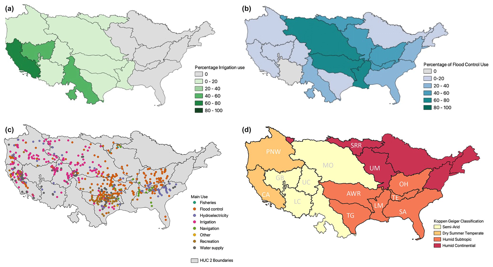
Figure 1 Maps depicting the percentage of the storage capacity used for irrigation (a) and flood control (b), point locations of all dams in ResOpsUS colored by the main use (c) and the aridity of all the regions with the 12 main regions in this study outlined (d). Panels (a) and (b) are calculated by summing up the total storage capacity of dams with irrigation (a) or flood control (b) as their main use and dividing that number by the storage capacity in each region. Grey shading in both denotes regions that do not have any irrigation or flood control dams. Dams that did not have a main use are not mapped in panel (c). Panel (d) depicts the mode of the Köppen–Geiger climate index pixels to classify the regional climates for each HUC2. Panel (d) also contains the abbreviations of the basin names pulled from the USGS HUC2 watershed boundary dataset as denoted in Table 1.

Seasonal aggregation was done by grouping monthly fraction filled values and then taking the maximum, minimum and median across the different periods. Regional trends were calculated via Sen slopes using the fraction filled time series from 1980 to 2019. Sen slopes are the average of the slopes calculated between every set of points in a test dataset. This approach is more robust and less sensitive to outliers and end points compared to normal linear trends. All Sen slopes in this paper were calculated with a 95 % confidence interval, and a p value of 10 % (0.1) was used as significant. Trends in the monthly range were calculated by taking the range of each month and year (i.e., January 1980, February 1980, etc.) and then plotting all the monthly ranges across time. Sen slopes were calculated for these fits using the same 95 % confidence interval and a p value of 0.1.

2.3 Fraction filled anomaly and recovery ratio

The fraction filled anomaly is used to normalize storage by month (Eq. 2) so that we can compare drought impacts across regions. To start, we calculated the monthly (m) median FF value across the full period from 1980 to 2019 for each region (R), denoted as FF_R,m in Eq. (2). Then, every daily FF value was matched to the correct month so that we could calculate the difference between the daily value and the monthly median. Daily fraction filled time series were then further aggregated to monthly for the drought sensitivity and recovery analysis (Sect. 3.4).

$$\begin{array}{}\text{(2)}& {\mathrm{Anomaly}}_{\mathrm{R},\mathrm{d}}={\mathrm{FF}}_{\mathrm{R},\mathrm{d}}-{\mathrm{FF}}_{\mathrm{R},\mathrm{m}}\end{array}$$

We then quantified several metrics for each drought. First, we calculated the drought recovery time as the date on which the SSI or FF anomaly values were equal to or greater than the respective value at the start of the drought period. We then define the recovery ratio (RR) as the time it took the fraction filled anomaly to recover divided by the time it takes the SSI values to recover. Recovery ratio values less than 1 denote that the drought metric took longer to recover, and RR values greater than 1 show that the fraction filled anomaly took longer to recover.

3 Results

In this section, we present reservoir operating patterns seasonally (Sect. 3.1), over time (Sect. 3.2) and in response to drought (Sect. 3.3). In all the cases, we study the 14 bold regions in Fig. 1d that have sufficient data in ResOpsUS. In our discussion section, we summarize these behaviors, explore relationships between climate, operational uses and observed behaviors and compare them to common assumptions made by reservoir modeling studies.

Table 1 USGS HUC2 names and corresponding abbreviations used in all the figures. Basins are labeled from the western to eastern coasts.

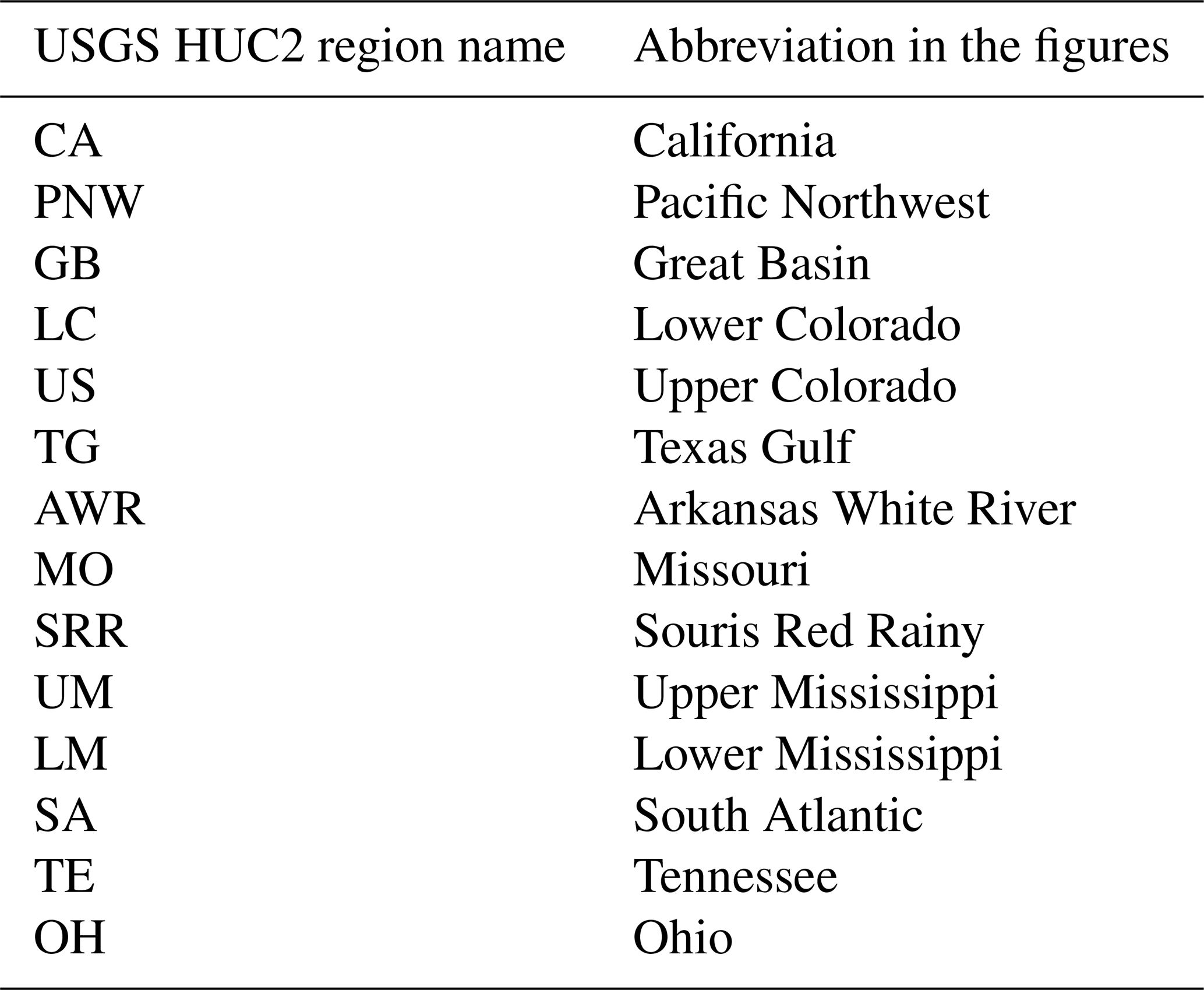
Figure 1 maps reported reservoir usages nationally along with aridity to provide additional context for discussion. As shown in Fig. 1c, reservoirs in the CONUS domain have a variety of primary uses ranging from flood control, irrigation, recreation, water supply, navigation, fisheries and others. There are some clear regional trends. The western US is dominated more by irrigation uses, while flood control is the dominate usage along and east of the Mississippi River (Fig. 1a and b). In ResOpsUS, the flood control and irrigation main uses are the most numerous. However, there are also many navigation, hydroelectricity, water supply and recreation reservoirs across the CONUS domain (Fig. 1c). The irrigation and water supply main uses are typically west of the Mississippi, while flood control main use reservoirs exist throughout the entirety of the CONUS domain. California has the largest percentage of irrigation reservoirs, with the Great Basin and Rio Grande following close behind (Fig. 1a). There are no irrigation reservoirs in the dataset east of the Mississippi, where the climate is more humid (Fig. 1d). Comparatively, flood control reservoirs have the highest concentration along the Mississippi Basin. All the regions apart from the Lower Colorado have at least one flood control reservoir (Fig. 1b). Navigation reservoirs are concentrated in the southeastern portions of the CONUS domain, especially in the Ohio, South Atlantic, Lower Mississippi and Texas Gulf regions. Hydroelectricity reservoirs are most common in the Tennessee Basin and the South Atlantic.

Spatial patterns in reservoir purpose correlate with national climate patterns. Figure 1d shows the aridity indices according to the Köppen–Geiger index (Kottek et al., 2006). The Köppen–Geiger index uses annual precipitation and temperatures to classify climates into four main groupings: tropical, dry, continental and polar. Of these, the continental United States contains all except polar. For each HUC2 region, we used zonal statistics to calculate the number of pixels in each Köppen–Geiger climate index to quantify the regional climates. The northeastern United States is humid continental, meaning that seasonal precipitation variability is small and temperatures are relatively cool (less than 22 °C) all year. The southeastern United States is primarily humid subtropical, which has warm and moist conditions in the summer months and makes summer the wettest season and winter the driest in comparison. The midwestern United States is semi-arid with warm summers, snowy winters and large diurnal temperature swings. These regions also observe more precipitation in the winter months, while the summer months are marked by drier spells. Finally, the West Coast is dry summer temperate, which is characterized by moderate temperatures and changeable, rainy weather in the winter as well as hot and dry summers.

Outside of the Pacific Northwest and California regions, it gets more humid as you move from west to east across the United States. The most arid regions exist in the southwestern United States, and the coasts are much more humid. While not all regions have sufficient operation data for analysis, the 12 regions that are included do span dry summer temperate regions (California), semi-arid regions (Upper Colorado, Missouri, Great Basin, Lower Colorado), humid continental regions (Souris Red Rainy) and humid subtropical regions (Texas Gulf, Arkansas White Red, Lower Mississippi, Ohio, South Atlantic, Tennessee).

3.1 Spatial patterns in reservoir operations

In this section, we quantify spatial patterns in regional reservoir operations using four main metrics: (1) the monthly median fraction filled, (2) interannual variability in the monthly fraction filled (referred to as the monthly storage range), (3) monthly operating ranges (i.e., the difference between the maximum and minimum storage within a given month) and (4) the month of the highest median fraction filled and the highest fraction filled range for over 400 dams in these 14 regions.

Based on the great variability in aridity and reservoir purpose across the US, we expect to see regional differences in both reservoir levels and seasonal operating patterns. Figure 2 shows the median fraction filled values across the 40-year study period from 1980 to 2019. Overall, we see that more arid regions and irrigation-dominated regions tend to have larger median fraction filled values (greater than 0.6), yet all median fraction filled values do not exceed 0.8. This suggests a potential flood control storage of around 20 %. Conversely, the more humid regions with greater flood control percentages in the southeast have median fraction filled values that sit between 0.2 and 0.5. These results align well with the historical analysis of Graf (1999), who investigated how storage capacity and population density changed in the CONUS domain, specifically looking at reservoir use (although this analysis was based on static reservoir values as opposed to operational data).

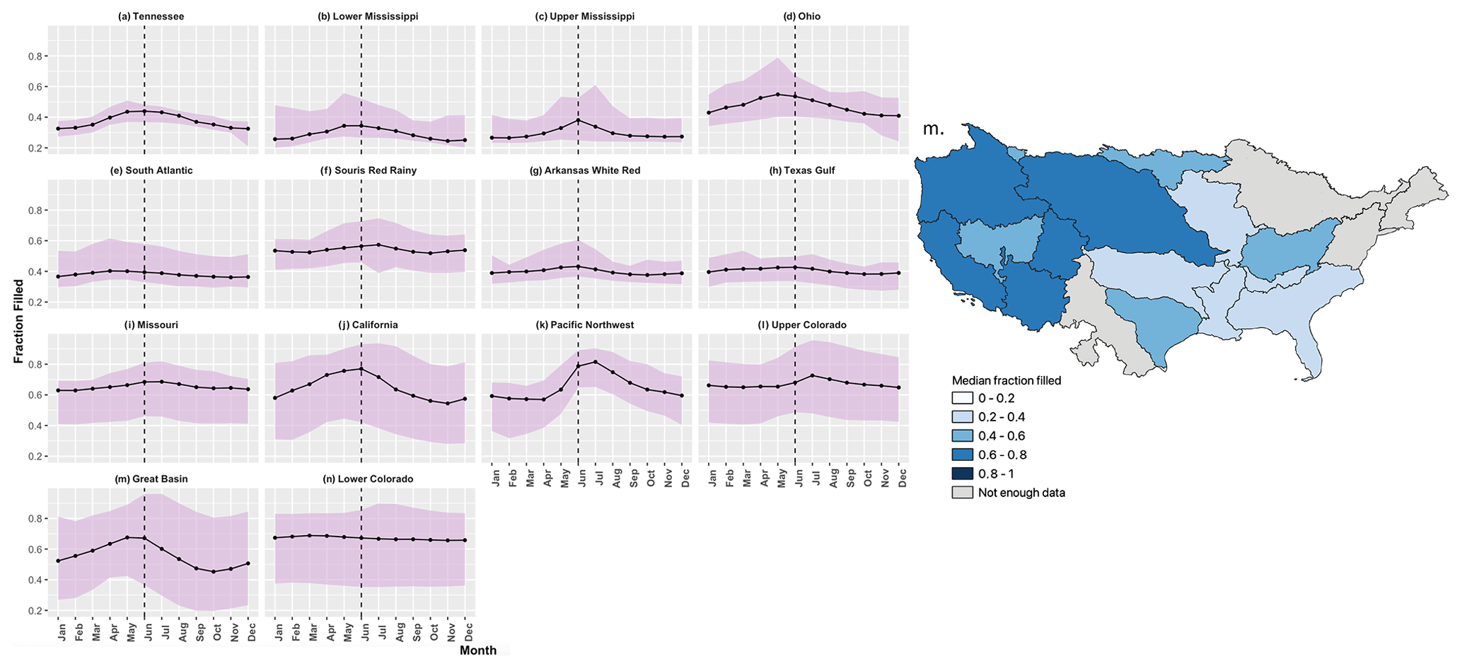
Figure 2 Median monthly reservoir fraction filled (black line) and the monthly fraction filled range in purple shading from 1980 to 2019 (a–l) and median fraction filled values (m). The vertical dashed line corresponds to the month of June as a reference point. Regions are organized from the most humid to most arid regions.

The monthly maximum and minimum fraction filled values illustrate regional differences in seasonal operating patterns. Five of the regions have median storage peaking in June. Irrigation-dominated regions (Missouri, Upper Colorado, Lower Colorado, Great Basin, Souris Red Rainy, Pacific Northwest, Fig. 2f and i–n) have maximum storage peaks later than June (typically in July and August). This could correspond to water being held in storage later in the year to support summer irrigation in periods where precipitation is more limited. Conversely, regions with more flood control reservoirs (Ohio, Tennessee, Lower Mississippi, Texas Gulf, Arkansas White River, South Atlantic, Fig. 2a–g) generally have median fraction filled peaks in May. The Upper Mississippi (Fig. 2c) is an outlier here as the median fraction filled values peak in June instead of early May, which could suggest the influence of other reservoir types. We also see that more humid regions tend to have less month-to-month variation in the median fraction filled, while more arid regions like the Upper Colorado and the Great Basin have stronger seasonal trends.

The interannual variability in the monthly fraction filled (referred to as the monthly storage range) for the 40-year period is shown by the shaded areas in Fig. 2. Monthly storage ranges generally follow the same overall trends seen in the median values (i.e., the monthly range peaks in the same month as the median fraction filled values peak). However, the monthly range peaks in the spring in the more humid basins (Fig. 2a–d). Souris Red Rainy and Upper Mississippi both have a drop in May right before the median fraction filled peak in June. Comparatively, the maximum range for Lower Colorado is in July and the lower bound of the median fraction filled values stays the same from season to season. In general, the biggest monthly ranges are seen in arid basins except for seasonal peaks in Ohio.

Next, we consider the operational storage range. This is the range of storage with each month (i.e., the maximum minus minimum storage in a single month). Note that this is different from the monthly storage range, which is the maximum and minimum storage seen in a given month across our 40-year study period. Figure 3 plots the median monthly operating range for all the years as well as the maximum and minimum by basin. Small values here indicate little variability within the storage values for a given month, while large values can indicate significant filling or draining. Except for the South Atlantic region (Fig. 3d), the variability in the operating ranges goes down as aridity increases (moving from top left to bottom right in Fig. 3). While the minimum operating range stays constant across all the seasons, the maximum operating range typically occurs in the spring months, with peaks for humid and flood-control-dominated regions. Irrigation regions have peak operating range values in the summer (July and August). Notably, Lower Colorado has a slight peak in April, yet the seasonal line is flat.

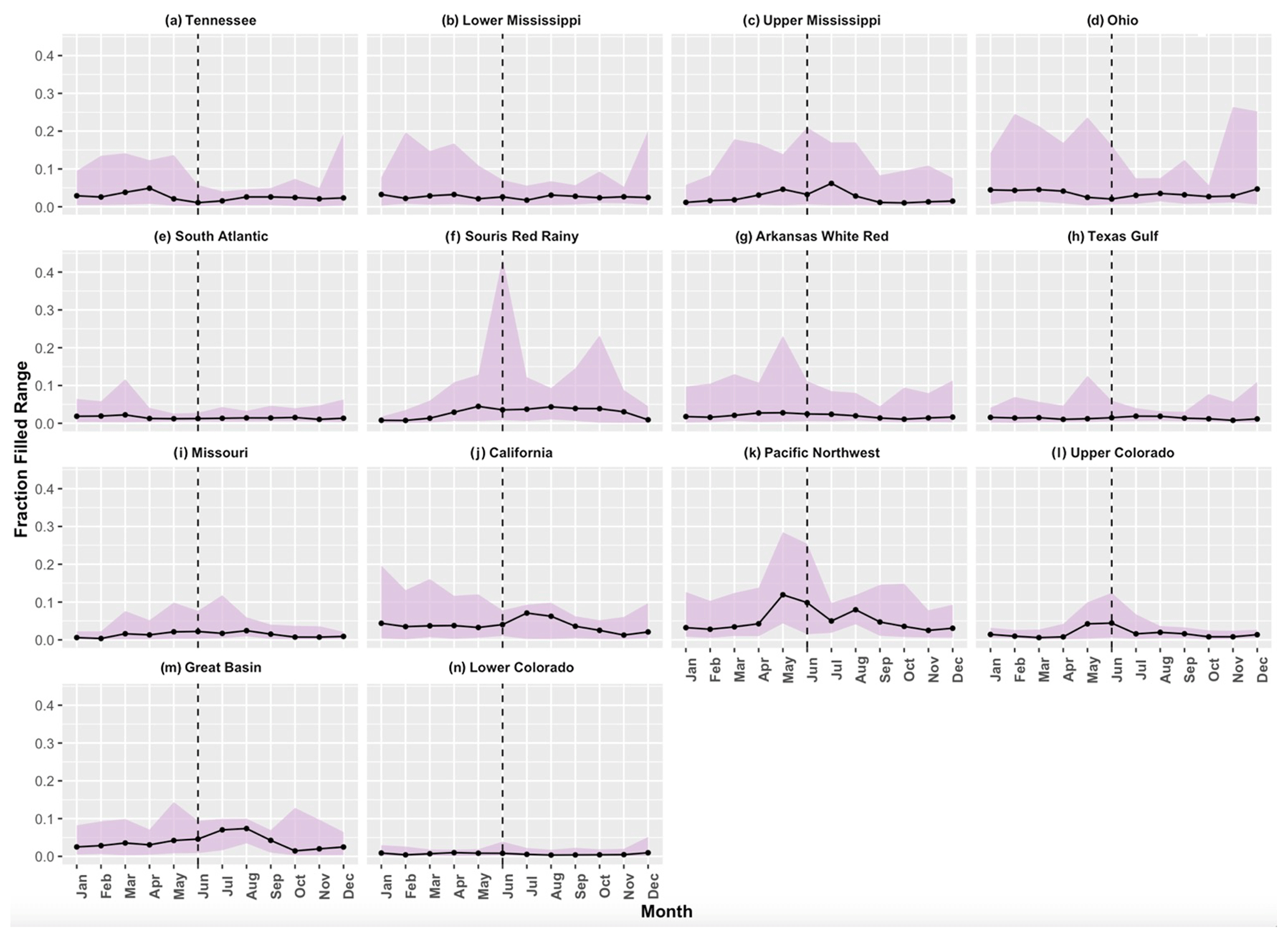
Figure 3 Median operating range of reservoir storage (black line) per month and the maximum and minimum range values for each month in purple shading. The dashed line corresponds to the month of June to provide a point of reference. Median, maximum and minimum values are calculated for the monthly storage range (daily maximum–daily minimum storage) each month across the 1980–2019 water year period. As in Fig. 2, regions are organized from the most humid to most arid regions (a–i).

We observe two main types of behavior for the median operating range: basins with clear seasonal variability and those without. The Tennessee, Lower Mississippi, Ohio, South Atlantic, Arkansas White Red, Texas Gulf, Missouri and Lower Colorado (Fig. 3a–d, f–h and l) basins all have very little monthly variability in their operating ranges. Most of these regions are humid, and the dominant storage purpose is flood control. The Lower Colorado is an outlier as it is arid and irrigation-dominated. However, this dynamic is to be expected as the flows in the Lower Colorado are heavily regulated and controlled by the Colorado River Compact. California, Upper Colorado, Great Basin, Pacific Northwest, Upper Mississippi and Souris Red Rainy (Fig. 3e and i–k) all have a clear seasonal cycle in the operating ranges. All these regions exhibit a peak in the median operating range during the spring or summer months and, except for Souris Red Rainy, Upper Mississippi and Pacific Northwest, are predominately semi-arid. Peaks in the spring would be consistent with reservoir filling in snowmelt-dominated basins (Souris Red Rainy, Pacific Northwest and Upper Colorado), while summer peaks may reflect drawdown for irrigation in the summer (California, Upper Mississippi and Great Basin). Finally, the operational range variability (purple shading) peaks based on the main use with non-irrigation uses (mainly in the eastern US) peaking in winter and irrigation uses (the western US) in late spring and summer.

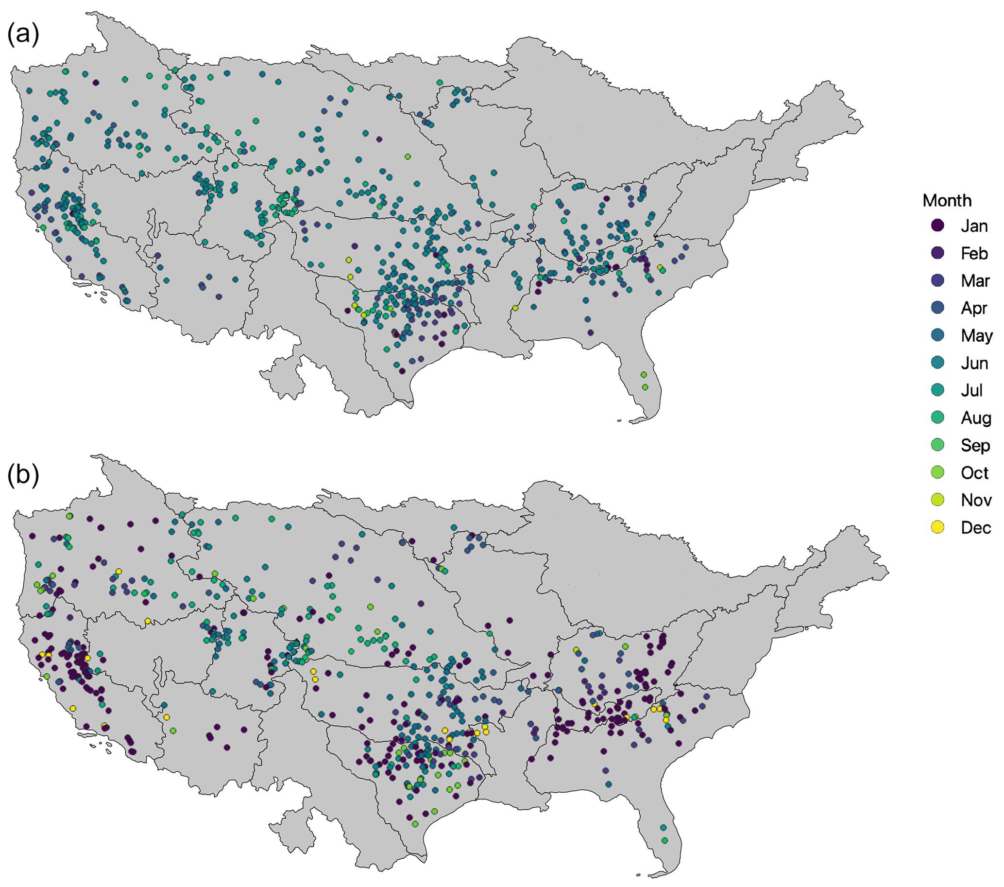
Figure 4 Maps of individual dams colored by the month of the highest fraction filled median (a) and the largest fraction filled range (b).

To complement the regional analyses and disentangle the effect of storage capacity on the regional analyses, we plotted the month of the greatest median fraction filled (Fig. 4a) and the month of the largest fraction filled range (Fig. 4b). Overall, most individual dams have peaks in the median fraction filled in the spring. The largest fraction filled median occurs mostly in April for reservoirs east of the Mississippi and June for reservoirs west of the Mississippi. These regional differences align with the priority of either flood control (eastern reservoirs) or irrigation (those in the western US) as well as seasonal differences between snowmelt-dominated and rainfall-dominated basins. The large median FF in the western US late into summer most likely supports summer irrigation. Another large subset of reservoirs has median FF peaks in winter (November–February). These reservoirs are all located in the southeastern US and mid-Atlantic regions. The peak in the median fraction filled during this period most likely aligns with flood control after the fall storm season.

The monthly fraction filled range map (Fig. 4b) shows similar trends: large ranges in the winter months for the eastern and southeastern US and large ranges in the summer for the western US. These two main periods align with the necessary operations for flood control (primarily during the winter months) and irrigation (primarily during the summer and early fall months). That said, there is a large subset of reservoirs across the western US (primarily in California, the Lower Colorado and the Pacific Northwest) that have fraction filled range peaks in the winter months due to increased storage for water use in the spring.

3.2 National storage trends

Over the past 100 years, reservoir storage capacity has steadily increased across the US (Fig. 5a). In the 1950s, the total storage capacity rapidly increased with a construction boom (Benson, 2017; Ho et al., 2017; Di Baldassarre et al., 2018). Starting in 1975, dam construction began to slow down as environmental regulations increased and prime locations for large dams were increasingly taken. By the 1980s, the total storage capacity in the CONUS domain levelled off and the era of large dam building came to an end.

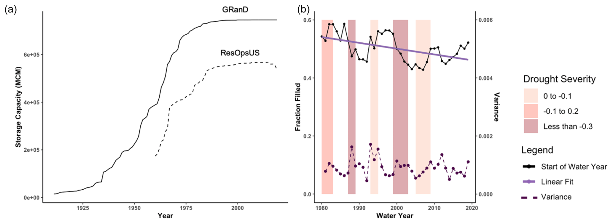
Figure 5 (a) Total storage capacity reported by GRanD (solid line) and the storage capacity of 679 large dams in ResOpsUS (dashed). (b) The reservoir fraction filled value on 1 October from the ResOpsUS data from the 40-year period from 1980 to 2019 (interannual fraction filled). The lavender line is the linear fit through this entire period of record with a slope of −0.002 fraction filled per year and a p value of 0.01. The colored rectangles depict the drought periods calculated over the entire CONUS domain, with darker colors referring to more severe droughts (SPI values less than −0.3) and medium-dark (SPI values between −0.1 and −0.3) and lighter bars to the least severe droughts (values between 0 and −0.1).

As previously noted, the ResOpsUS dataset that we are using for our analysis includes data for 678 dams, roughly 85 % of the dams with a storage capacity greater than 1000 MCM and 77 % of the total storage in the CONUS domain (Fig. 5a, dashed line). While all the storage is not included in this dataset, Fig. 5a shows that there is a similar temporal trend in the reservoir storage covered in ResOpsUS and the total national storage (i.e., rising most rapidly up to 1980 and then levelling off). It should also be noted that reservoir storage capacity decreases in ResOpsUS after 2020 are due to missing data in recent years for the ResOpsUS dataset and are not an indication of dam removal (recall that the ResOpsUS storage capacity is reporting only the capacity of those dams that have data each year).

While reservoir storage capacity has remained steady over the past 40 years (1980–2019), the fraction filled has steadily decreased over this period (denoted by the lavender trend line in Fig. 5b). There can be many reasons for storage declines (i.e., sedimentation, increased demand, evaporative losses or decreased precipitation). However, broadly speaking, decreases in the fraction filled are correlated with climatic shifts as illustrated by drops after extreme drought periods (colored in maroon). Conversely, during non-drought periods and less severe droughts (pale pink), we see that reservoirs can recover, although not fully (as indicated by the declining trend). Overall, reservoir storage peaks at 60 % fraction filled in 1989 and drops all the way to 43 % in 2007. In more recent years, there is some recovery of the fraction with a final value of 53 %. We also plot the reservoir fraction filled variance over time (Fig. 5b; note that this is the annual variance of daily fraction filled values, referred to as annual storage variance). Annual storage variance peaked in 1995 and does not demonstrate the same clear trend, as was shown with storage. Variance generally increases during drought periods and is lower during non-drought periods. This means that variance is peaking during the same periods and that storage is dropping, suggesting an inverse relationship between variance and storage levels.

3.3 Regional storage trends

Next, we evaluated regional storage trends for the 14 regions that had 40 % or more storage covered. We calculate a linear trend using values from 1980 to 2019 for the first month of the water year (October) (Fig. 6a–l) to evaluate carryover storage. From this, we identified three behavior types: (1) low interannual variability (Fig. 6a–h), (2) more interannual variability but no significant linear trend (Fig. 6i–k) and (3) high variability and trends (Fig. 6l–n). Tennessee, Lower Mississippi, Ohio, South Atlantic, Arkansas White Red and Texas Gulf display slightly linear interannual fraction filled trends and have very small changes in interannual storage. These regions are dominated by flood control, navigation and hydroelectricity, main uses that require stable heads to generate use. Additionally, these regions are all humid (Fig. a–d) and semi-arid (Fig. 6f and g). This is consistent with the results of Sect. 3.1, which showed that the more humid and flood-control-dominated parts of the country tend to have lower storage values overall and less variability in storage. Of these, the Upper Mississippi, Lower Mississippi, Tennessee and Ohio regions have statistically significant linear trends (p<0.05) and are all positive, suggesting that there has been an increase in storage over time.

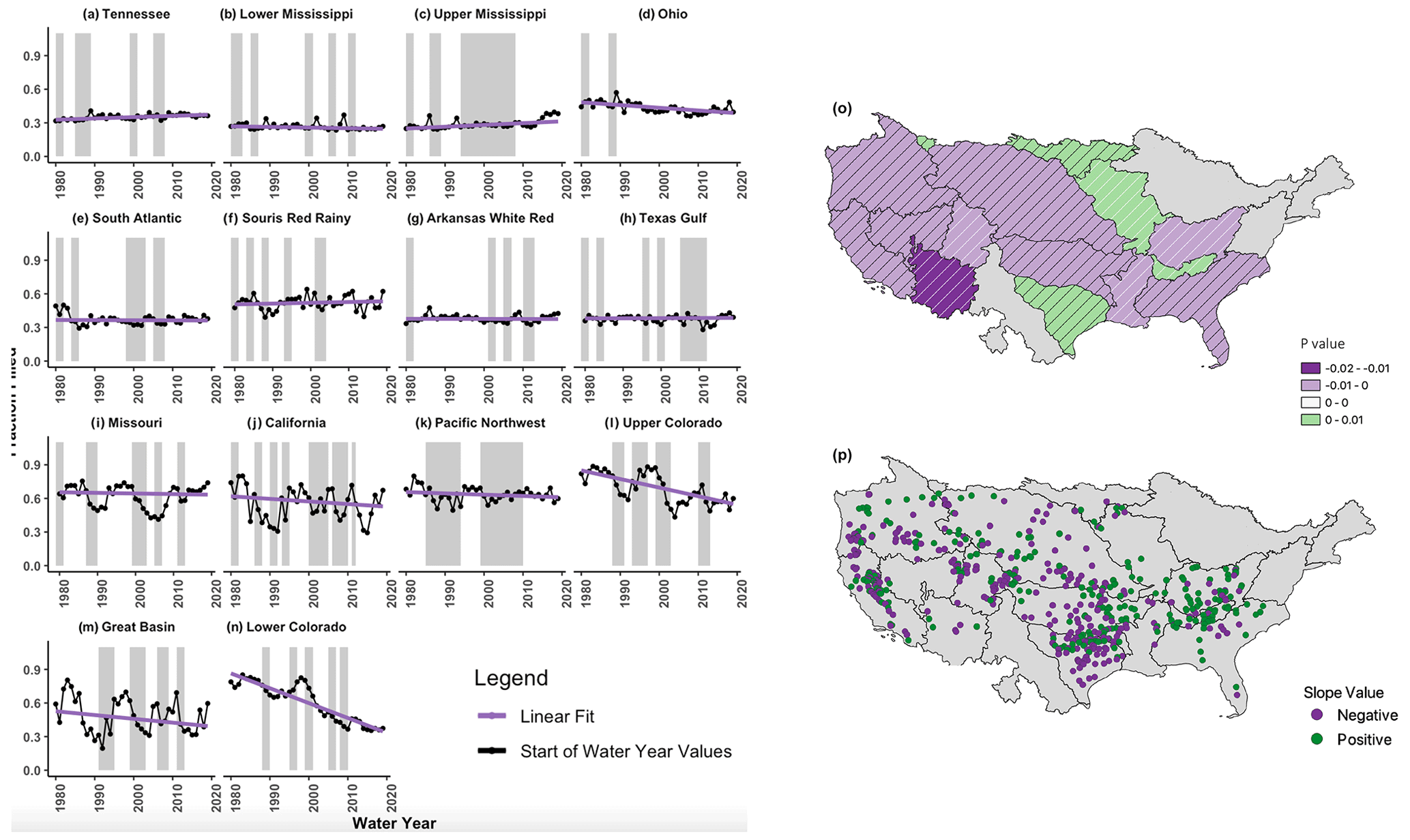
Figure 6 Regional interannual fraction filled from October 1980 to October 2019 (a–l) and the associated map of the Sen slope values (m). The black lines are the October storage, and the lavender lines are the linear trend. The maroon boxes correspond to periods where SPI values, calculated over the entire relevant basin, were less than −0.3. Sen slopes (m) range from −0.013 (dark purple) to 0.0011 (green) with similar trends based on aridity. P values are calculated using a 95 % confidence interval. The horizontal white and black lines denote the regional p values that are above the 5 % probability (10 %–50 % for the white lines and >50 % for the black lines) threshold and are not considered statistically significant.

The second set of regions (Souris Red Rainy, Missouri, California, Pacific Northwest and Great Basin, Fig. 6g and i–k) all have large interannual variability but very slight linear trends that are not statistically significant. These regions have larger carryover storage, are mainly water-supply- and irrigation-dominated and are all more arid (i.e., semi-arid and dry summer temperate in the case of California and the Pacific Northwest). Conversely, Upper Colorado (Fig. 6l) has both high interannual variability and a statistically significant negative storage trend. In all these regions, reservoir storage appears to be strongly influenced by dry periods as shown by the shading in Fig. 6.

Finally, the Lower Colorado (Fig. 6n) does not fit into any of these groupings. This basin has a strong linear trend and little interannual variability (note that the fraction filled does not return to a value each year but rather plummets). This semi-arid basin mainly consists of irrigation, water supply and hydroelectricity main uses, yet we only see the interannual variability similar to non-irrigation reservoirs. This is likely because storage in the Lower Colorado is dominated by storage in Lake Mead as the Hoover Dam holds a large fraction of the total storage in the basin. Additionally, the Colorado River Compact dictates the releases and therefore the storage in Lake Mead, which has seen historic lows due to the mega-drought (Williams et al., 2022) and increased aridification trends (Overpeck and Udall, 2020) in the southwestern United States. That said, the strong negative trend in the Lower Colorado is a cause for concern and has been a topic of much discussion as the western US is currently experiencing a mega-drought (Fig. 6m) (Williams et al., 2022).

We also calculated the Sen slopes for the individual dams included in our regional analysis and mapped them in Fig. 6p. Across the CONUS domain, all the basins have both positive and negative storage trends. Basins with predominately positive trends in Fig. 6o such as Ohio and Tennessee also have numerous dams with negative fraction filled trends. Additionally, basins such as the Lower and Upper Colorado have positive slopes. Therefore, the bulk of the storage trends seen in Fig. 6o are dominated by the dams with the largest storage capacity. Figure 6p also depicts regions where the overall trend in Fig. 6o is slightly skewed from what is observed regionally. In fact, regions with more flood control and navigational uses (the eastern and southeastern US) have more positive fraction filled trends, while regions with more irrigation and water supply uses (the western US) have more negative trends. The Texas Gulf region stands out in this regard as the region is dominated by both water supply and flood control uses, and therefore there are both positive and negative storage trends.

We also observe the degree of storage drawdown that happens over drought periods regionally (i.e., the grey-shaded periods in Fig. 6). In all the basins, storage decreases during the dry periods. However, in humid regions and regions where flood control is the dominant reservoir purpose, these declines appear to be much smaller. This is consistent with previous results showing that these locations maintain less storage overall and have smaller operational ranges. Semi-arid basins with higher levels of irrigation and water supply uses have sharper drawdown patterns during drought. Again, this is consistent with previous results showing a larger operational range and carryover storage in these areas. In most cases, reservoir storage goes down during drought. There are, however, notable periods in all the regions where storage increases. Examples include Souris Red Rainy and Texas Gulf during the drought periods in the early 1980s and the drought in the early to mid 1990s for the Upper and Lower Colorado. A more detailed regional analysis is required to understand the causes of these increases.

In addition to overall storage trends, we evaluate whether there have been historical trends in the operational range (i.e., the difference between maximum and minimum storage in a given month) for each year. For every region, we calculate a time series of monthly operational ranges and fit linear Sen slopes to each month to evaluate whether the operational range is increasing or decreasing for that month over time. Figure 7 depicts these trends as bar plots colored by positive (blue) or negative (pink) and shaded by statistically significant (dark) or non-significant (light) p values at a significance of 5 %. Positive trends mean that the interannual operational range is increasing over time, and negative trends mean that this interannual operational range is decreasing over time. Firstly, we will look at distinctions between positive and negative trends without accounting for the significance. Regions such as Souris Red Rainy, California, Lower Mississippi, Upper Mississippi and Great Basin have more positive months than negative months, indicating that, overall, their interannual operational range is increasing over time. Conversely, basins such as Tennessee, Ohio, South Atlantic, Arkansas White Red, Texas Gulf, Upper Colorado and Missouri have interannual operational ranges that are decreasing over the past 40 years. Lower Colorado has an even split between positive and negative trends, suggesting a seasonality in the increase (April) and decrease (July, August and October) of the operational range trends. Missouri and Lower Mississippi are unique examples of these two trends as the majority of their interannual operational range slopes are quite small except for 2 months: December for Lower Mississippi and May for Missouri. It is possible that changes in the operating range could be solely attributed to shifts in demand and inflow (which could still be captured with static rule curves), or it could be the case that the operating policies are also shifting over time.

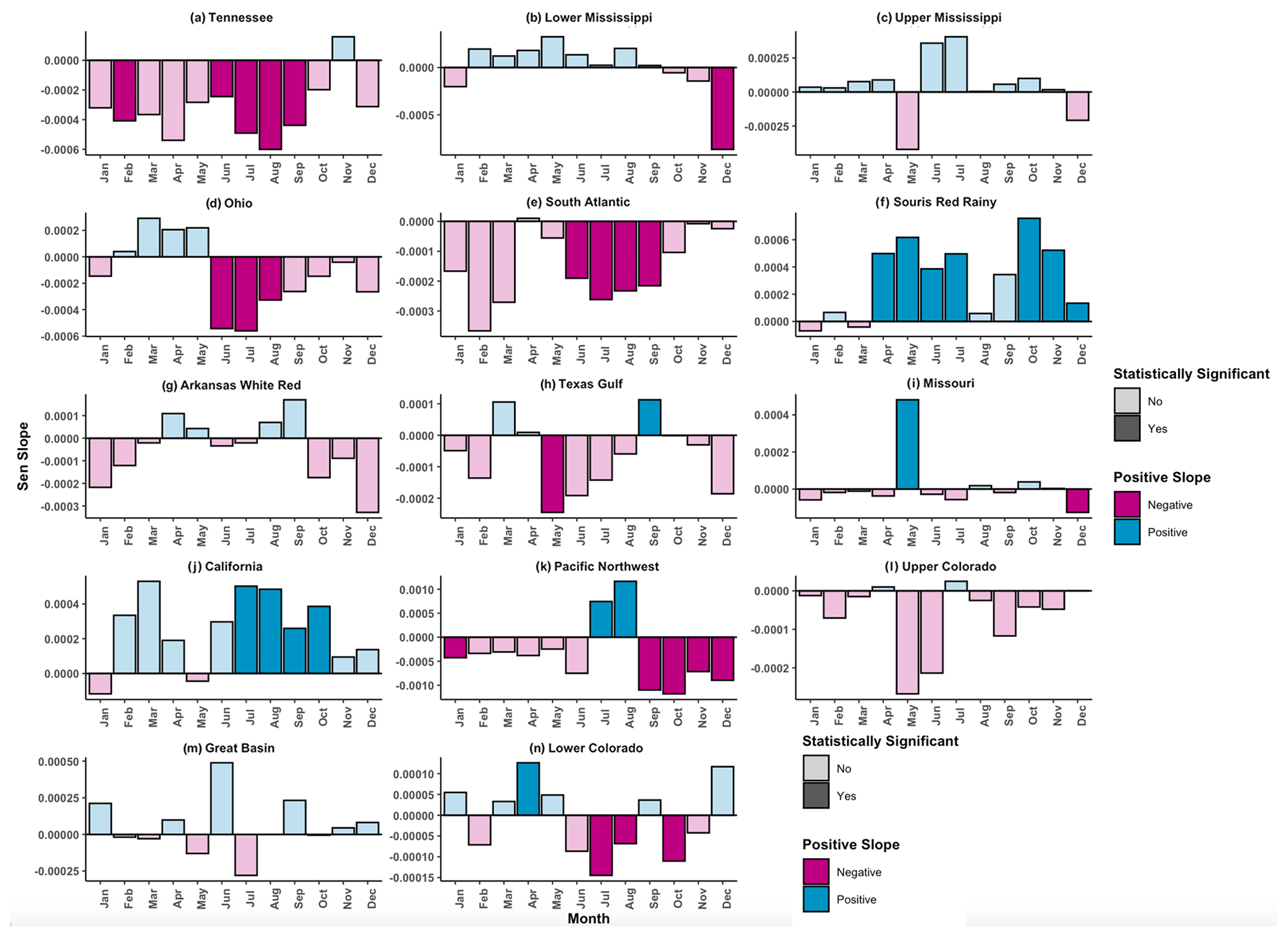
Figure 7 Trends in the monthly fraction filled range from 1980 to 2019. Bars are colored as not statistically significant (light) and statistically significant (dark). The p value is calculated with a 95 % confidence interval, and significant values are less than 0.1. Each panel pertains to a specific region within the United States, where most of the storage capacity is covered (greater than 50 %). The panels are organized from the wettest to driest regions.

To account for the statistical significance, we group the behaviors into four categories. First, the Tennessee, South Atlantic, Ohio, Pacific Northwest and Lower Colorado regions (Fig. 7a, d, e, k and n) have three or more negative monthly trends that are statistically significant. All these regions apart from the Pacific Northwest have statistically significant negative trends in July and August, with Tennessee, Ohio and the South Atlantic having statistically significant trends in the summer months (June–August). The Pacific Northwest has decreasing trends in the fall and winter, with increasing trends in July and August potentially to open storage for irrigation. Apart for the Lower Colorado and the Pacific Northwest, these regions are primarily humid with low carryover storage. The second set contains regions that have predominately positive trends and are greater than or equal to three statistically significant trends (Souris Red Rainy and California, Fig. 7f and j). Of these regions, Souris Red Rainy has statistically significant positive trends in the spring and fall, while California only has statistically significant trends in the fall. The positive and statistically significant values indicate that these regions have seen increases in the interannual operational range during these seasons compared to their counterparts with negative trends. The last group contains regions without statistically significant trends (Lower Mississippi, Upper Mississippi, Texas Gulf, Great Basin, Arkansas White Red, Upper Colorado and Missouri (Fig. 7b, c, g–i, l and m). While these basins may have 1 month of statistically significantly trends (December and May), the lack of statistically significant values does not allow us to definitely align them with operations.

4 Discussion

In this section we synthesize the detailed results presented above to characterize regional differences in operating regimes (Sect. 4.1) and evaluate where our results agree and disagree with common assumptions that are made in large-scale reservoir modeling approaches (Sect. 4.2). The intent here is to provide a summary of the behaviors we should expect to see from large-scale models (which can be useful for both model evaluation and model parameterization) and to highlight where current approaches may be the most systematically biased.

4.1 Characterizing regional patterns in reservoir operating regimes

Our results highlight strong regional differences in reservoir operations. More humid regions generally have a lower total storage capacity and a lower median fraction filled, while more arid regions have a higher median fraction filled. This difference is consistent with findings by Ho et al. (2017) and Graf (1999) and is due to regional differences in streamflow regimes and reservoir purposes. Irrigation and water supply are often the main reservoir purposes in the western, more arid United States, while the eastern, more humid United States contains more flood control and hydropower uses. Additionally, the more humid regions also have lower monthly storage ranges without strong seasonal cycles. This is due in part to the lower storage capacity dams without strong intra-annual storage changes (Patterson and Doyle, 2018; Benson, 2017). This is complemented by seasonal increases in fraction filled variance in the winter and spring for humid and flood-control-dominated regions to support flood control and navigation operations and ensure stable reservoir storage. Conversely, more arid regions with higher concentrations of irrigation reservoirs have spring and summer peaks to support runoff in snowmelt-dominated basins (Upper Colorado, Pacific Northwest and California) and irrigation uses. This direct relationship between variance and storage seen in Fig. 5 could be caused by two things: (1) increased seasonal demand which is leading to releases that are fluctuating more to meet demand and greater drawdown (as seen in the Lower Colorado region) or (2) environmental releases which have shifted operating policies away from a constant release strategy.

Flood control reservoirs are generally characterized by lower fraction filled values and less clear seasonal variability. Median fraction filled values generally peak in May for flood control reservoirs (which could be due to reservoir operators maintaining low storage in the spring to prevent downstream flooding). Additionally, there are decreased monthly variations in flood control reservoirs as operators are attempting to keep their storage levels consistent with the maximum storage range peaking in the spring. Flood control and hydropower reservoirs have the most stable seasonal median fraction filled with small peaks in the spring and winter as operators bring storage back to normal operating values. When observing the month of the highest median fraction filled and the month of the highest fraction filled range (Fig. 4a and b, respectively), these two trends appear to be constant over time, as we see that most reservoirs have a median fraction filled peak in April or May for eastern reservoirs with operational range peaks in January.

Conversely, irrigation and water supply reservoirs have a much stronger seasonal cycle and different peak storage timing. While flood control reservoirs have median fraction filled peaks in May, irrigation reservoirs generally have fraction filled peaks in June (and, in some cases, even late summer). Irrigation reservoirs are also dominated by strong filling cycles with strong seasonal trends in their monthly storage ranges. Irrigation and water supply uses have monthly storage range peaks in the summer to support water supply for humans and plants during periods where precipitation and runoff are limited. This strong seasonality shows up in the operating range spread, which is quite large in irrigation-dominated basins with a wider spread during late spring and early summer (the main irrigation period in the United States). The median fraction filled peak month (Fig. 4a) demonstrates that, for most of the western US, this relationship holds. When looking at the month of the highest operational range, we see that the range is highest in late summer and early fall for all western basins apart from California and the Pacific Northwest, where flood control operations have a higher priority. Regions have delayed peaks in their operations due in part to irrigation being separate from filling as operators strive to hold water later in the summer when supply is not as consistent. Irrigation and water supply dominated regions also have a larger interannual variability when looking between water years (Fig. 3).

Across the CONUS domain, we find a strong negative trend in reservoir storage which is consistent with previous studies (Adusumilli et al., 2019; Zhao and Gao, 2019; Hou et al., 2022; Randle et al., 2021). Only the Tennessee and Upper Mississippi basins have had a statistically significant positive trend in storage over the past 40 years. This is due in part to the abundance of flood control and navigation reservoirs and increases in streamflow which potentially combine to increase the total storage held in this region (Naz et al., 2018). When looking at the individual dams in Fig. 6p, we see that more flood-control-dominated regions (Tennessee, Ohio, South Atlantic and California) have a large proportion of dams with a positive trend over the past 40 years. Declining storage trends are concerning in regions such as the Lower Colorado and Upper Colorado, where the impact of a mega-drought is threatening water supplies (Williams et al., 2022) and the region is expected to continue aridifying under future projections (Overpeck and Udall, 2020). Similarly, in the Lower Mississippi, low storage levels can threaten the operation of navigation reservoirs that support the transport of goods longitudinally in the United States.

Throughout our study we find the Lower Colorado to be unique in many regards. The Lower Colorado has very low seasonal variations in median fraction filled values and operating ranges, with seasonal peaks during the summer (consistent with irrigation uses) and operational range peaks in April (consistent with flood control uses). Additionally, the spread of the operational range is quite similar to flood control reservoirs, as it is kept quite steady with few to no monthly variations. Finally, the fraction filled variance peaks in the winter and early spring with no monthly changes. These dynamics are most likely a result of the fact that most of the water supply comes from reservoir releases from the Upper Colorado basin. The negative storage trend is concerning as this basin is water-limited and extractions routinely outpace the inputs from the Upper Colorado. Combined with the current mega-drought (Williams et al., 2022) facing the western United States and the aridification trends of the southwestern US (Overpeck and Udall, 2020), there is an large increase in vulnerability to drought in this region that can be expected to continue.

4.2 Comparison to common reservoir assumptions

Historically, global hydrologic models employ a range of simplifications to represent reservoir operations. This is done out of necessity given the lack of consistent datasets on reservoir operations. Here, we used the unique analysis that is made possible by the ResOpsUS dataset to discuss the potential limitations of simplifying assumptions. The intent is to highlight where more complicated approaches in reservoir operations may make a significant difference in estimated storage and water supply.

Two widely cited approaches by Hanasaki et al. (2006) and Haddeland et al. (2006) rely on static reservoir characteristics such as the maximum storage capacity, main reservoir purpose and average annual inflow to parameterize reservoir operations. These two models rely on similar simplifying assumptions: (1) assume that dead storage (the amount of water that cannot be pulled from the reservoir) is 10 % of the maximum storage, (2) releases are based on storage at the start of the operational year, (3) downstream demand is weighted by the maximum storage capacity in the basin, and (4) monthly water demand per sector is used to determine releases. Hanasaki et al. (2006) further assume that the modeled storage capacity is 85 % of the observed maximum storage capacity and that reservoir operations are determined by a single primary purpose. Haddeland et al. (2006) take a slightly more complex approach allowing for multiple reservoir operations (i.e., water supply, hydropower, irrigation or flood control) and employing retrospective rule curves where the year-end releases are used to determine reservoir releases at the current time step. The assumptions employed by both of these approaches are a significant limitation for the complexity they can represent. However, they are also well suited for data-sparse regions and global models.

We found that water supply reservoirs do have more carryover storage than hydropower or navigation reservoirs. However, the resulting impact of this carryover storage varies greatly with respect to climate. When combined with irrigation dams, the impact of this carryover storage in water supply reservoirs in the western US is more pronounced than in the more humid basins such as the Texas Gulf or Tennessee basins. This suggests that climate is the key driver in the carryover storage (more carryover storage in arid regions compared to humid regions) as well as the other regional reservoirs. On an individual basis, we do see that selected water supply reservoirs in more humid basins appear to have similar characteristics to those in more arid basins (Fig. 4), yet overall there is a distinct difference between humid and arid basins. This difference on the basin scale is more likely due to reservoir operations in series, which causes water supply reservoirs to be operated more like the reservoirs around them (flood control and navigation in the east and irrigation in the west). That said, we do note that classification of operational policies by main purpose should be taken with a degree of uncertainty as this is the main purpose and many reservoirs are multipurpose (i.e., an irrigation dam that contains flood storage).

We also see quite distinct storage patterns between irrigation-dominated reservoirs in the western US and non-irrigation reservoirs in the eastern US. However, our results show significant seasonal variability in operations which cannot be explained by seasonal differences in inflow alone. Approaches that use constant operating policies throughout the year are likely to miss seasonal patterns in both fraction filled and operating ranges.

There have been recent efforts that take a more complex approach and use historical reservoir time series to derive reservoir operations (Turner et al., 2020, 2021; Yassin et al., 2019). In these methods, operations are derived from observed reservoir time series and the number of generalized assumptions are limited. Yassin et al. (2019) employ a set of five storage zones in which reservoir releases will shift based on the storage zone and incoming streamflow. Like Turner et al. (2021), these zones are set based on historical time series, yet unlike Turner et al. (2021), these zones are set via an exceedance probability or optimization function instead of harmonic regressions. Therefore, Yassin et al. (2019) assume that the operational zones will stay static into the future. Comparatively, Turner et al. (2020, 2021) (which are both based on the same model) assume that releases are based upon the week of the year, the incoming inflow that week and the start-of-week storage. The harmonic regression is fit to historical time series to determine the operational range. This method is also readily extrapolated to other reservoirs with similar operational purposes and hydrologic seasonality.

Still, previous research has found that rule curves can underestimate seasonal dynamics by smoothing out peaks (Turner et al., 2021). Our results demonstrate large seasonal fluctuations in the eastern reservoirs which could be underestimated when only looking at smoothed curves such as in Turner et al. (2020). We also show that operational ranges vary throughout the year, indicating the need for dynamic zoning of reservoirs as seen in Yassin et al. (2019). This may also be necessary for multipurpose reservoirs or those with large interannual storage (primarily those in the western US and California). The seasonalities in the operational ranges (Fig. 2) show that eastern regions with more flood control reservoirs (and those that rely heavily on forecasted inflows and multipurpose reservoirs in irrigation-dominated basins) would be prime candidates for the models similar to Yassin et al. (2019) as they allow for storage targets for a variety of uses. Unfortunately, this method will continue to be limited by data gaps until reservoir time series are consolidated in one centralized database.

Another common assumption in large-scale models is that operating policies do not change over time. For example, all the above reservoir operations, Hanasaki et al. (2006), Haddeland et al. (2006), Yassin et al. (2019) and Turner et al. (2021), are trained on historical data and assume that operational range bounds stay consistent. Our results show that not only are there long-term trends in total reservoir storage but that there are also trends in the reservoir operating ranges over time. In more arid basins such as the Upper Colorado, Souris Red Rainy and California regions, the operational range has been increasing. In more humid basins, such as the Tennessee, Ohio and South Atlantic regions, operational ranges have been decreasing, which is supported by Patterson and Doyle (2018), who show that operational ranges have shifted.

Many reservoir studies assume that reservoir storage stays between 10 % and 85 % of that maximum storage capacity (Yassin et al., 2019; Voisin et al., 2013). This assumption is supported in all 14 of the regions that we looked at in the CONUS domain. In fact, all the regions have a minimum fraction filled by at least 20 % and in most cases 40 %. This suggests that, in practice, reservoir storage stays well above the 10 % threshold. Providing 10 % as the lowest storage value may not be a problem if reservoirs are not hitting that threshold but could also lead to simulations that overestimate the actual operational range. Specifically, our analysis demonstrates that most of the eastern basins (with primary uses of flood control, hydropower and navigation) have long-term median storage ranges that stay well within this assumed operating range. However, in the western regions, we see fraction filled values quite close to 0.85 (Fig. 1a–l).

Finally, many reservoir studies use static datasets such as GRanD for their maximum storage capacities. There are 100 dams in our study, where observed storage values exceed the reported maximum storage values in GRanD. While some of these could directly relate to periods when the reservoir was overtopped, it could also be that the maximum storage capacity in GRanD is inaccurate due to data gaps. In the GRanD documentation, Lehner et al. (2011) specifically state that, if the maximum storage capacity was not reported, the reported storage capacity or the minimum storage capacity is used instead.

5 Conclusion

Here we use the first national dataset of direct reservoir observations (ResOpsUS) to develop a comprehensive summary of historical reservoir operations across the US and to compare the relationships we get from direct observations to common assumptions made in large-scale reservoir parameterizations. Our results show strong regional differences in reservoir behaviors as well as trends over time. The median storage peaks are in winter and spring for the eastern US and in summer for the western US. Conversely, minimum storage typically occurs in early summer in the eastern US and in winter in the western US. Over our 40-year study period (1980–2019), five of the regions we evaluated had statistically significant decreasing storage trends. Of these five, the Lower Colorado is the most negative due to the ongoing mega-drought in the past 20 years (Williams et al., 2022). The Tennessee region is the only basin with a positive storage trend, potentially due to increased streamflow across the eastern US and decreasing operational ranges (Naz et al., 2018). Overall, operational ranges have been increasing over time in more arid regions and decreasing in more humid regions.

Our operational range analysis can be useful both for deriving rule curves as well as a calibration tool to assess whether the modeled operations align with historical shifts. Similarly, the seasonal shifts in operational ranges shown here are important for understanding when in the year reservoirs are most actively filling and draining. The spatial variability in our seasonal results highlights the need for complex zoning or rule curves.

While many of our findings agree with the general assumptions that are commonly made about different types of reservoirs (e.g., storage and release timing differences for flood control vs. irrigation reservoirs), the spatial and temporal complexity of our results highlights the potential biases that can be introduced with simplified operational representations. For example, our evaluation of seasonal trends, something that has not been explored previously with direct observations at this scale, highlights seasonal differences operating behaviors throughout the year which may not be captured by models that assume constant operations. Similarly, long-term trends in reservoir storage and operating ranges point to operating policies that also shift over time. The results presented here can be a benchmark for large-scale reservoir models to (1) understand the limitations of common assumptions and (2) quantify the potential biases in data-limited regions where this type of comparison is not possible.