Advance prediction of coastal groundwater levels with temporal convolutional and long short-term memory networks

Prediction of groundwater level is of immense importance and challenges coastal aquifer management with rapidly increasing climatic change. With the development of artificial intelligence, data-driven models have been widely adopted in hydrological process management. However, due to the limitation of network framework and construction, they are mostly adopted to produce only 1 time step in advance. Here, the temporal convolutional network (TCN) and models based on long short-term memory (LSTM) were developed to predict groundwater levels with different leading periods in a coastal aquifer. The initial data of 10 months, monitored hourly in two monitoring wells, were used for model training and testing, and the data of the following 3 months were used as prediction with 24, 72, 180, and 360 time steps (1, 3, 7, and 15 d) in advance. The historical precipitation and tidal-level data were incorporated as input data. For the one-step prediction of the two wells, the calculated R² of the TCN-based models' values were higher and the root mean square error (RMSE) values were lower than that of the LSTM-based model in the prediction stage with shorter running times. For the advanced prediction, the model accuracy decreased with the increase in the advancing period from 1 to 3, 7, and 15 d. By comparing the simulation accuracy and efficiency, the TCN-based model slightly outperformed the LSTM-based model but was less efficient in training time. Both models showed great ability to learn complex patterns in advance using historical data with different leading periods and had been proven to be valid localized groundwater-level prediction tools in the subsurface environment.

1 Introduction

As the economic development and population escalate in the coastal area, the fresh groundwater needs to continue mounting, and seawater intrusion has posed a great threat to the availability of portable water resources globally (Baena-Ruiz et al., 2018). In the United States, Mexico, Canada, Australia, China, India, South Korea, Italy, and Greece, with dense population, many coastal aquifers have experienced salinization caused by seawater intrusion (Barlow and Reichard, 2010; Park et al., 2012; Pratheepa et al., 2015; Zhang et al., 2017; Lu et al., 2013). Protection projects such as aquifer replenishment can be constructed to alleviate seawater intrusion by artificially increasing groundwater recharge in the aquifer more than what occurs naturally (Abdalla and Al-Rawahi, 2012; Lu et al., 2019). The replenishment programs have been operated in the developed areas such as Perth, Western Australia, and California, USA (Garza-Díaz et al., 2019). The infrastructures tend to be costly and out of reach for many developing countries. A reliable seawater intrusion monitoring and the predicting system is still essential and is recognized as the most effective way of keeping fresh water from seawater contamination (Xu and Hu, 2017).

In the past several decades, conventional numerical models have been widely utilized to simulate and predict groundwater fluctuation dynamics and chemical variations (Batelaan et al., 2003; Dai et al., 2020; Huang et al., 2015; Li et al., 2002). However, the difficulty of acquiring extensive hydrological and geological data and setting reasonable boundaries limits its application to seawater intrusion management. Meanwhile, the method is not suitable for simultaneously adopting updated monitoring data and producing real-time prediction. Under such circumstances, where the data source is scarce, artificial intelligence technology has been proposed in groundwater dynamic predictions. Artificial neutral networks (ANNs) have been greatly improved and has become a robust tool for dealing with groundwater problems where the flow is nonlinear and highly dynamic in nature (Maier and Dandy, 2000). The conventional network model generally has defects such as high computational complexity, slow training speed, and failure in retaining historical information, making it hard to be enrolled in the long-term time-series prediction (Cannas et al., 2006; Mei et al., 2017). To solve this problem, researchers upgraded the conventional networks by integrating them with methods like a genetic algorithm (Mehr and Nourani, 2017; Ketabchi and Ataie-Ashtiani, 2015), singular spectrum (Sahoo et al., 2017), and wavelet transform (Gorgij et al., 2017; Seo et al., 2015; Zhang et al., 2019). Singular spectrum analysis and wavelet transform can help to preprocess the time-series data before they are put into the neural networks to improve prediction accuracy and efficiency.

With computing capacity development, deep learning (DL) has emerged as a very powerful time-series prediction method. The DL models are particularly suitable for time series of big data because they can automatically extract complex patterns without feature extraction preprocessing steps (Torres et al., 2018). However, the generally fully connected networks are not effective in capturing the temporal dependence of time series (Senthil Kumar et al., 2005). Therefore, more specialized DL models, such as recurrent neural networks (RNNs) (Rumelhart et al., 1986) and convolutional neural networks (CNNs) (LeCun et al., 1998) have been adopted in the field of time-series prediction (Feng et al., 2020). Different from the backpropagation (BP) neural network where the information flows from the input to the output layer in one direction, the RNN preserves the information from the previous step as input to the current step with loops (Coulibaly et al., 2001). This allows the RNN to handle time-series and other sequential data, but it is generally not straightforward for a long-term calculation in practice (Bengio et al., 1994). Therefore, the enhanced RNN model, long short-term memory (LSTM) is proposed and capable of processing high variable-length sequences, even with millions of data points (Fischer and Krauss, 2018; Kratzert et al., 2019). As one of the best deep neural network models in time-series predicting, the LSTM has been widely used in the prediction of temporal variations such as stock market predictions (Fischer and Krauss, 2018), rainfall–runoff (Dubey et al., 2021), and groundwater level (Solgi et al., 2021). Despite substantial progress in hydrology prediction, these networks still have issues of low training efficiency and low accuracy (Zhan et al., 2022).

More recently, a variant of the CNN architecture known as temporal convolutional networks (TCNs) has gained popularity (Bai et al., 2018). The prominent characteristic of a TCN is its ability to capture long-term dependencies without information loss (Cao et al., 2021). Meanwhile, it joints a residual block structure to fix the disappearance of the gradient in the deep network structure (Chen et al., 2020). With proper modifications, the TCN is quite genetic and can easily be used to build a very deep and extensive network in sequence modeling. In earth science, the TCN has been successfully applied to time-series prediction tasks, including multivariate time-series predicting for meteorological data (Wan et al., 2019), probabilistic predicting (Chen et al., 2020) and wind speed predicting (Gan et al., 2021). Researchers suggest that the TCN convincingly has the advantage in popular DL models across a broad range of sequence modeling tasks (Borovykh et al., 2018; Chen et al., 2020; Wan et al., 2019). Another important subject is that these networks are mostly used to predict variables in only one step, which is not enough for the prediction of hydrological information in management. Researches have adopted the method to predict the trends of El Niño–Southern Oscillation (ENSO) and sea temperature (Yan et al., 2020; Jiang et al., 2021). However, the potential of TCNs has not been investigated in the sequencing model of the hydrogeology field. Therefore, it is worthy to explore their prediction abilities in leading periods.

The objective of this study is to develop real-time advance prediction climate–hydro hybrid data-driven models of groundwater level in the coastal aquifer based on TCNs and LSTM. The hourly processed tidal-level, precipitation and groundwater-level data in monitoring wells of Laizhou Bay are adopted as training data. The trained models are then utilized to predict the groundwater-level variation in an advance period of 1, 3, 7, and 15 d. The two models were further compared in view of accuracy and efficiency. The rest of the paper is organized as follows. Section 2 introduces the study area and observational data. Section 3 illustrates the detailed concepts of the TCN and LSTM, the experimental model settings, and model evaluation criteria. Section 4 presents the predicted results and discussions. Finally, the paper is concluded in Sect. 5.

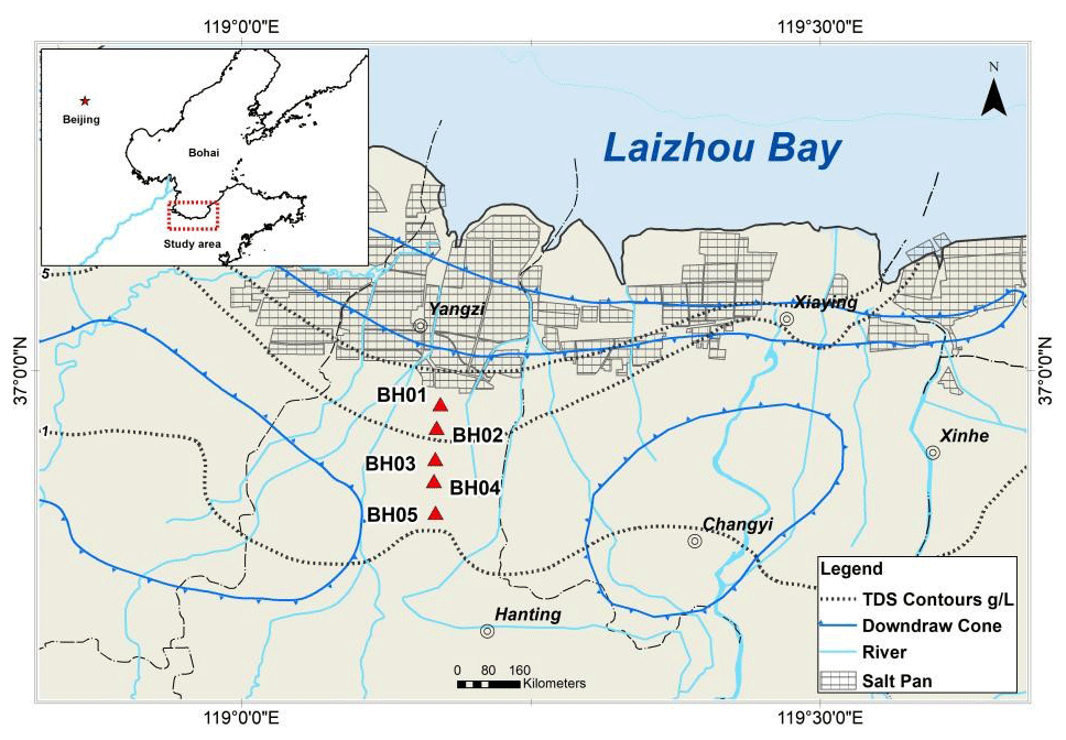
Figure 1 Schematic figure of the study area with monitoring wells BH01–BH05.

2 Study area and data processing

2.1 Site description

The study area is located on the south coast of Laizhou Bay, along the Yangzi to Weifang section in the Shandong province of China (Fig. 1). Laizhou Bay is one of the first regions in China to be significantly impacted by seawater intrusion since the 1970s (Han et al., 2014; Zeng et al., 2016). The area is a coastal plain, which contains a series of Cretaceous to modern sediments that cover the Paleozoic basement. The sedimentary facies of coastal aquifer are alluvium, pluvial, and marine sediments from south to north (Han et al., 2011). According to the research of Xue et al. (2000), there have been three seawater intrusion and regression events in the sea area of Laizhou Bay since the upper Pleistocene. The transgression in the early upper Pleistocene formed the third marine aquifer containing sedimentary water. This brine was formed by evaporation and concentration of ancient seawater and re-dissolution and mixing of salt (Dai and Samper, 2006; Zhang et al., 2017). The monitoring wells BH01–BH05 are distributed in the study area along a cross-section perpendicular to the coastline. Among the wells, BH01 and BH05 have relatively integrated data in time and are distributed on the two sides of the cross profile with distinguished annual variation patterns, which are selected as examples for the developed models.

2.2 Data collection and pre-processing

The precipitation and tidal level are selected as the primary factors to affect the groundwater dynamics in the coastal area. The data in the period of 2011 to 2012 with groundwater-level observations of two wells are combined as the input of the DL models. A total of 28 836 data items are collected for monitoring wells. The variations of groundwater level and tidal level with precipitation are shown in Fig. 2. The rainfall is concentrated from June to September and in shortage from December to April. The tide in the study area is irregular, mixed with a semi-diurnal variation. In the experiments, 10 months of data from October 2011 to July 2012 is first extracted for model training and testing. The rest of the data from August 2012 to October 2012 is used to test model prediction accuracy.

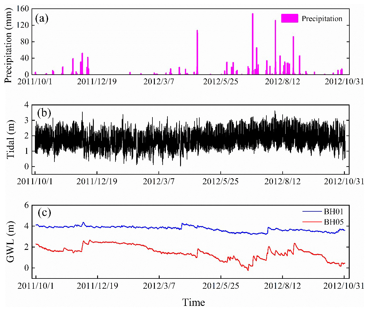
Figure 2 Time series of the variables in the study, including (a) precipitation, (b) tide, (c) groundwater level (GWL).

In addition, the magnitudes of meteorological and hydrological variables have obvious temporal variations. To reduce the negative impact on the model learning ability, especially on the speed of gradient descent, all variables are normalized to ensure that they remain at the same scale (Kratzert et al., 2019). This pre-processing method ensures the stable convergence of parameters in the developed TCN- and LSTM-based models and improve the simulation accuracy of the model. The normalization formula is as follows:

$$\begin{array}{}\text{(1)}& x_i^{\prime }={\displaystyle \frac{x_i-x_{\min }}{x_{\max }-x_{\min }}},\end{array}$$

where x_i represents the original data in time i; x_max and x_min are the maximum and minimum variable values, respectively. The output of the network is retransformed to obtain the final groundwater-level prediction, which is an inverse data-scaling process.

3 Methodology

3.1 Temporal convolutional network

The TCN is first proposed for video action segmentation and detection by hierarchically capturing intermediate feature presentations. Then, the term is extended for sequential data for a wide family of architectures with generic convolution (Bai et al., 2018; Lea et al., 2017). Suppose that we have an input hydro-climate sequence at different times x₀, …, x_T; the goal of the modeling is to predict the corresponding groundwater level as outputs y₀, …, y_T at each time. The problem could transfer to build a network f that minimizes the function loss between observations and actual network outputs L [(y₀, …, y_T), (${\widehat{y}}_{\mathrm{0}}$, …, ${\widehat{y}}_T$)], where ${\widehat{y}}_{\mathrm{0}}$, …, ${\widehat{y}}_T=f(x_{\mathrm{0}}$, …, x_T). Currently, a typical TCN consists of dilated, causal 1D full-convolutional layers with the same input and output lengths. With a TCN, the prediction y_t depends only on the data from x₀ and x_t and does not include the future data from x_t and x_T (Yan et al., 2020). With the three key components of a TCN, it has two distinguishing characteristics: (1) the TCN is able to map the same length of output as the input sequence in the RNN; (2) the convolution involved in TCNs is causal, eliminating the influence of future information on the output.

3.1.1 Causal dilated convolutions

In the TCN, the first advantage is accomplished by the architecture of a 1D full-convolutional network (FCN). Different from the traditional CNN, the FCN transforms the fully connected layers into the convolutional layers for the last layers, preserving the same length of output as that of the input (Long et al., 2015). As shown in Fig. 3a, the length of the hidden input layer and the length of the output layer is the same. Some zero padding is needed in this step by adding additional zero-valued entries with a kernel size length of 1 in each layer. The kernel size is the number of successive elements that are used to produce one element in the next layer.

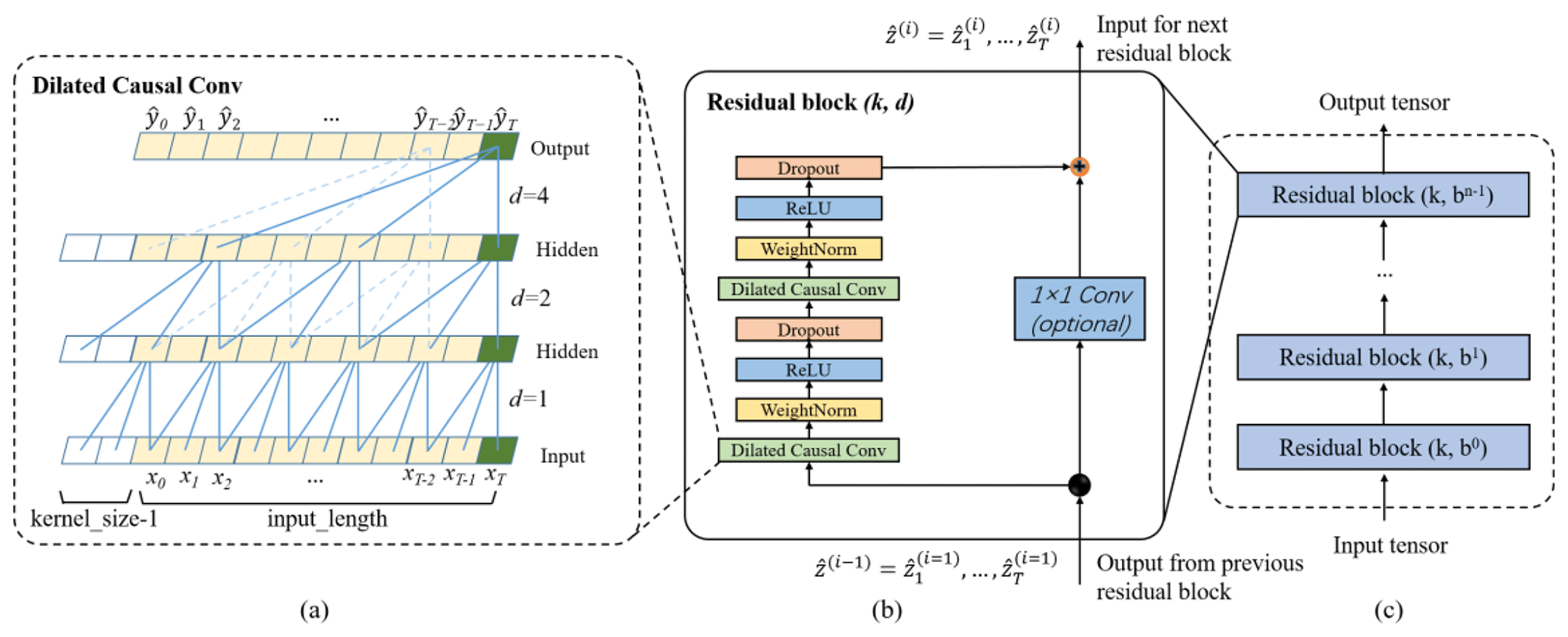
Figure 3 Architectural elements in the proposed TCN. (a) The structure of causal dilated convolution. (b) The TCN residual block – a 1×1 convolution is added when residual input and output have different dimensions; (c) framework of residual connection in the TCN.

To avoid information leakage from the future (after time t), the TCN uses causal convolution instead of standard convolution, where only the elements at or before time t in the previous layer are adopted into the mapping of the output at time t. Further, the dilated convolution is employed to capture long-term historical information by skipping a given step size (dilation factor d) in each layer. For example, the dilation factor d increases from 1 to 4 with the evolution of the network depth (n) in an exponentially increasing pattern. In this way, a very large receiving domain is created and all the historical records in the input can be involved in the prediction model with a deep network.

3.1.2 Residual connections

In a high-dimensional and long-term sequence, the network structure could be very deep with increasing complicity and cause a vanishing gradient. To solve this issue, a residual block structure is introduced to replace the simple 1D causal convolution layer so that the designed TCN structure is more generic (He et al., 2016). The residual block in a TCN is represented in Fig. 3b. It has two convolutional layers with the same kernel size, dilation factor and non-linearity. To solve non-linear models, the rectified linear unit (ReLU) is added to the top of the convolutional layer (Nair and Hinton, 2010). The weight normalization is applied between the input of hidden layers (Salimans and Kingma, 2016). Meanwhile, a dropout is added after each dilated convolution for regularization (Srivastava et al., 2014). For all connected inner residual blocks, the channel widths of input and output are consistent. However, the width may be different between the input of the first convolutional layer of the first residual block and the output of the second convolutional layer of the last residual block. Therefore, a 1×1 convolution is added in the first and last residual blocks to adjust the dimensions of the residual tensor to the same. The output of the residual block is represented by ${\widehat{Z}}^{\left(i\right)}$ for the ith block.

3.1.3 Structure of TCN

A complete structure of TCN is illustrated in Fig. 3c. It contains a series of proceeding residual blocks. The structural characteristics make TCN a DL network model very suitable for complex time-series prediction problems (Lara-Benítez et al., 2020). The main advantage of TCNs is that, similar to RNNs, they have flexible receptive fields and can deal with various length inputs by a sliding 1D causal convolution kernel. Furthermore, because a TCN shares a convolution kernel and has parallelism, it can process long sequences in parallel instead of sequential processing like an RNN, so it has lower memory usage and shorter computing time than a cyclic network. Moreover, RNNs often have the problems of gradient disappearance and gradient explosion, which are mainly caused by sharing parameters in different periods, while TCNs use a standard backpropagation-through-time algorithm (BPTT) for training, so there is little gradient disappearance and explosion problems (Pascanu et al., 2013). The detailed mathematical calculation and associated information of the TCN architecture are referred to in Bai et al. (2018).

3.2 Long short-term memory network

The LSTM is a special RNN model explicitly designed for long-term dependence problems. As shown in Fig. 4a, the RNN has a series of repeating modules that are recursively connected in the evolution direction of the sequence. The chain-like structure permits the RNN to retain important information in a “tanh” layer and produce the same length of output ${\widehat{y}}_t$ as input x_t. However, the short-length “remember time” is not enough for groundwater prediction. Especially for our hourly recorded data, a maximum time step of about 10 reported by Bengio et al. (1994) is unable to count the effect of annual, seasonal, and even daily groundwater variation. Different from the simple layer in the RNN, the LSTM has a more complicated repeating module with four interacting layers.

Figure 4 Graphical representation for (a) chain-like structure of the RNN by assigning x_t and ${\widehat{y}}_t$ as input and output. The self-connected hidden units allow information to be passed from one step to the next; (b) LSTM's memory block based on RNN. The hidden block includes three gates (input i_t, forget f_t, output o_t) and a cell state to select and pass the historical information.

The core idea of LSTM is the special structure to control the cell state in the module as shown in Fig. 4b. It includes a cell and an input gate i_t, a forget gate f_t, and an output gate o_t. The information can flow down directly along cells C without critical changes, therefore, preserving long-term historical messages (J. Zhang et al., 2018). The three gates control which data in a sequence are important to retain or discard, and protect the relevant information passed down in the cell to make predictions. The forget gate f_t has a sigmoid layer to determine which information is discarded with a value between 0 and 1. The lower the value, the less information is added to the cell state (Ergen and Kozat, 2017). In contrast to the forget gate, the input gate i_t decides what information to retain in the cell state. It is composed of two parts: a sigmoid layer and a tanh layer. The two layers are combined to govern which values will be updated by generating a new candidate value ${\stackrel{\mathrm{̃}}{C}}_t$. The old cell state C_t−1 can then be updated into the new cell state C_t with a weighted function. Finally, the output gate o_t determines which parts of the cell state should be passed on to the next hidden state. The detailed calculation of the LTSM can be referenced in Lea et al. (2016).

3.3 Experimental study

The TCN- and LSTM-based models were developed separately for monitoring wells BH01 and BH05. Due to the high complexity of the DL models, setting appropriate hyper-parameters for the developed networks is very important. Here, the impact of the size of the input window, the epoch number, and the batch size was tested with different convolutional architectures over the monitoring data (Lara-Benítez et al., 2020). The learning dataset is first divided into two parts: 80 % of the time-series data is used as the training set, and 20 % of the data is utilized as the testing set. The effect of different splitting strategies is further tested in Sect. 4. With the increase in the epoch numbers, the curve gradually approaches the optimal fitting state from the initial non-fitting state, but too many epochs frequently lead to over-fitting of the neural network (Afaq and Rao, 2020). Meanwhile, the number of iterations generally increases for updating weights in the neural network. Therefore, the number of epochs from 0 to 300 is evaluated. Batch size represents the number of samples between model weight updates (Kreyenberg et al., 2019). The value of the batch size is often set between one and hundreds. A larger batch size often leads to faster convergence of the model but may lead to a less ideal final weight set. To find the best balance between memory efficiency and capacity, the batch size should be carefully set to optimize the performance of the network model. Besides these parameters, the number of filters in the TCN-based and the hidden nodes in the LSTM-based model was tested within reasonable ranges as well.

The 1, 3, 7, and 15 d leading prediction experiments were further conducted to test the capacity of DL methods in predicting long-term groundwater levels in the coastal aquifer. To eliminate the randomness of model training, all experiments were repeated 5 times and the average values of each index were compared. In all experiments, the average absolute error (MAE) has been used as the loss function of networks (Lara-Benítez et al., 2020). The Adam optimizer has an adaptive learning rate that can improve the convergence speed of deep networks, which has been used to train the models (Kingma and Ba, 2015).

3.4 Evaluation of model performance

Two evaluation metrics, coefficient of determination (R²) and root mean square error (RMSE) are selected to quantify the goodness of fit between model outputs and observations (Zhang et al., 2020). The two criteria are calculated using the following equations:

$$\begin{array}{}\text{(2)}& {\displaystyle }& {\displaystyle }\mathrm{RMSE}=\sqrt{{\displaystyle \frac{\mathrm{1}}{N}}\sum _{i=\mathrm{1}}^N{\left(h_i-y_i\right)}^{\mathrm{2}}},\text{(3)}& {\displaystyle }& {\displaystyle }{R}^{\mathrm{2}}={\displaystyle \frac{\sum _{i=\mathrm{1}}^N{\left(h_i-\stackrel{\mathrm{‾}}{h}\right)}^{\mathrm{2}}-\sum _{i=\mathrm{1}}^N{\left(h_i-y_i\right)}^{\mathrm{2}}}{\sum _{i=\mathrm{1}}^N{\left(h_i-\stackrel{\mathrm{‾}}{h}\right)}^{\mathrm{2}}}},\end{array}$$

where h_i is the observed groundwater level at time i, y_i is the network prediction values at time i, $\stackrel{\mathrm{‾}}{h}$ is the mean of the observed groundwater levels, and n is the number of observations. The RMSE measures the prediction precision which creates a positive value by squaring the errors. The RMSE score is between [0, ∞]. If the RMSE approaches 0, the model prediction is ideal; R² measures the degree of model replication results, ranging between [−∞, 1]. For the optimal model prediction, the score of R² is close to 1.

4 Results and discussions

4.1 Hyper-parameter trial experiments

4.1.1 Experiments of the TCN-based model

The TCN-based model was built on the Keras platform using TensorFlow of Python as the backend. Taking the groundwater-level prediction dataset in well BH01 as an example, the trials were set up with a variety combination of different hyper-parameters in the TCN-based model as illustrated in Table 1. With the fixed number of epochs, the simulation results of 32 filters were better than that of 16 and 64 filters. Meanwhile, under the condition of 32 filters, the accuracy of the model decreased with the increasing batch size. The results of the 16 batch sizes were better than that of 32 and 64 batches. Based on the above experimental results, the influence of different numbers of epochs on the simulation was further explored when the filters were 32 and the batch size was 16, as shown in Fig. 5. The overall results of the model were improved when the number of epochs increased from 100 to 190, though the variation was not strictly linear, and the variations became stable with minor fluctuations when the number of epochs exceeded 200.

Table 1 The RMSE and R² values between the observed and predicted groundwater levels in well BH01 with different numbers of epochs, different numbers of filters, and different batch sizes. The bold values represent the optimal hyper-parameters with the smallest RMSE and the highest R² scores in the TCN-based model.

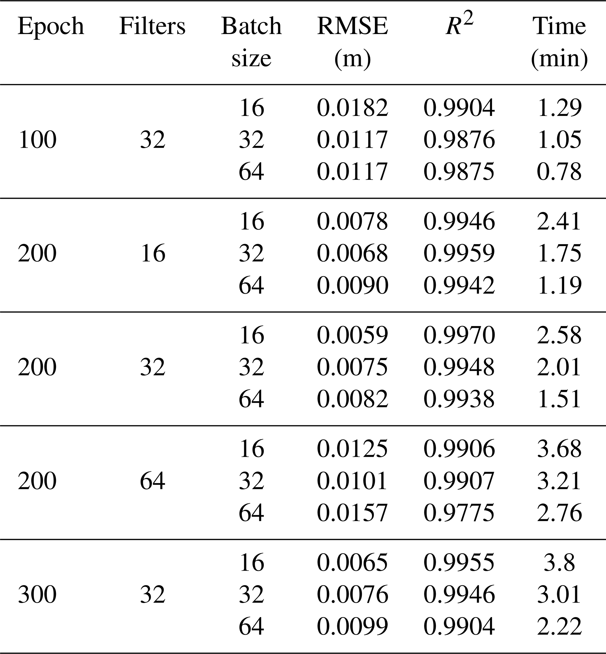
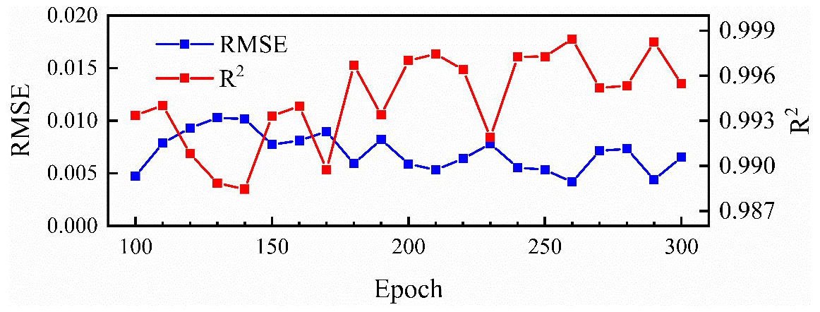
Figure 5 The variation of RMSE and R² values between the observed and predicted groundwater levels of well BH01 with the increasing number of the epochs when the number of filters is 32 and the batch size is 16.

4.1.2 Experiments of the LSTM-based model

The number of epochs and hidden nodes are two key parameters affecting the simulation accuracy of LSTMs (D. Zhang et al., 2018). Different hyper-parameter combinations were tested as well as in the proposed TCN-based model with groundwater levels in well BH01. The RMSE, R² and running time are shown in Table 2. With a fixed number of hidden nodes, the results of 100 and 200 epochs were better than that in the experiment with 300 epochs. A detailed variation of RMSE and R² values with the increasing number of hidden nodes and epochs is further illustrated in Fig. 6. The figure shows that the RMSE and R² have a decreasing and increasing trend separately when the number of epochs is greater than 150, but is reversed when it is larger than 240. The variations of RMSE and R² with increasing hidden nodes have similar changes. Though an insufficient number of neurons may decrease the learning ability of the network, the results indicate that increasing training hyper-parameters may not be necessary to ensure better prediction.

Table 2 The RMSE and R² values between the observed and predicted groundwater levels in well BH01 with different numbers of epochs and hidden nodes. The bold values represent the optimal hyper-parameters used in the proposed LSTM-based model.

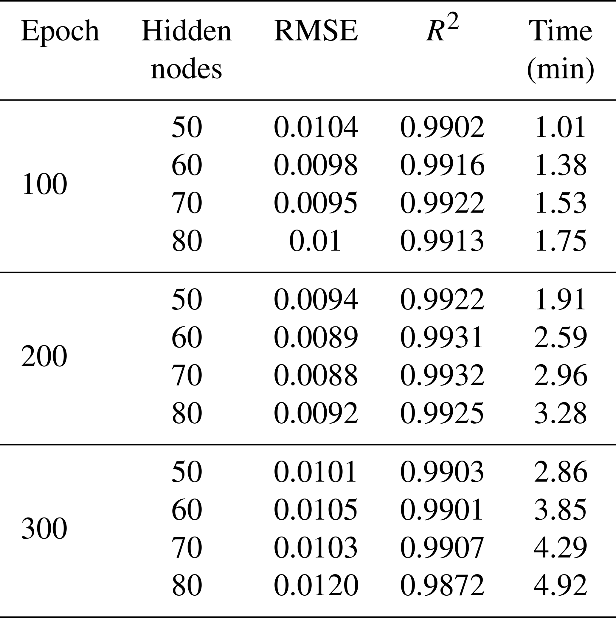
Figure 6 The variation of RMSE and R² values between the observed and predicted groundwater levels of well BH01 with an (a) increasing number of hidden nodes when the epoch equals 200 and an (b) increasing number of epochs when the hidden node is 50.

The trial experimental results present a similar fitting pattern shared by the two kinds of networks. The growing value of parameters dramatically increases the computational cost in the network. For example, the time cost from 50 to 80 hidden nodes has increased about 1.7 times in each iteration trial in the LSTM-based model. Finally, 200 epochs, 32 filters, and 16 batch sizes were chosen as the optimal parameters in the TCN. For the LSTM network, the number of epochs and hidden nodes were chosen as 200 and 70, respectively.

4.2 Model performance and evaluation

The optimal hyper-parameters of the proposed TCN-based model for groundwater-level predicting are shown in Table 1 (epoch = 200, filters = 32 and batch size = 16). Besides that, the kernel size in each convolutional layer is set as 6, and the dilations are 1, 2, 4, 8. For the LSTM-based model, the batch size is set to 148 with epochs = 200 and nodes = 70. The same hyper-parameters are then utilized to construct TCN and LSTM architectures for the prediction of groundwater level in different monitoring wells.

The one-step-ahead simulated groundwater level in the training and testing and prediction stages by the two models are shown in Fig. 7. For both models, the simulated values completely capture the variation of groundwater levels in monitoring wells with the overlapped plots. The R² and RMSE values of simulation results are listed in Table 3. In the prediction stage, the values of RMSE are 0.0019 and 0.0166 for BH01 and BH05, and the values of R² are larger than 0.999 in the prediction for the TCN-based model. For the LSTM-based model, the RMSE values are 0.0074 and 0.0588, and the R² values are 0.9957 and 0.9980. These metrics indicate that both models can “remember” the historical records and produce true observations. The simulation accuracy of TCN-based models is slightly higher than the LSTM-based models. In addition, the running time of the TCN-based model is 2.6 min, which is faster than that of the TCN-based model.

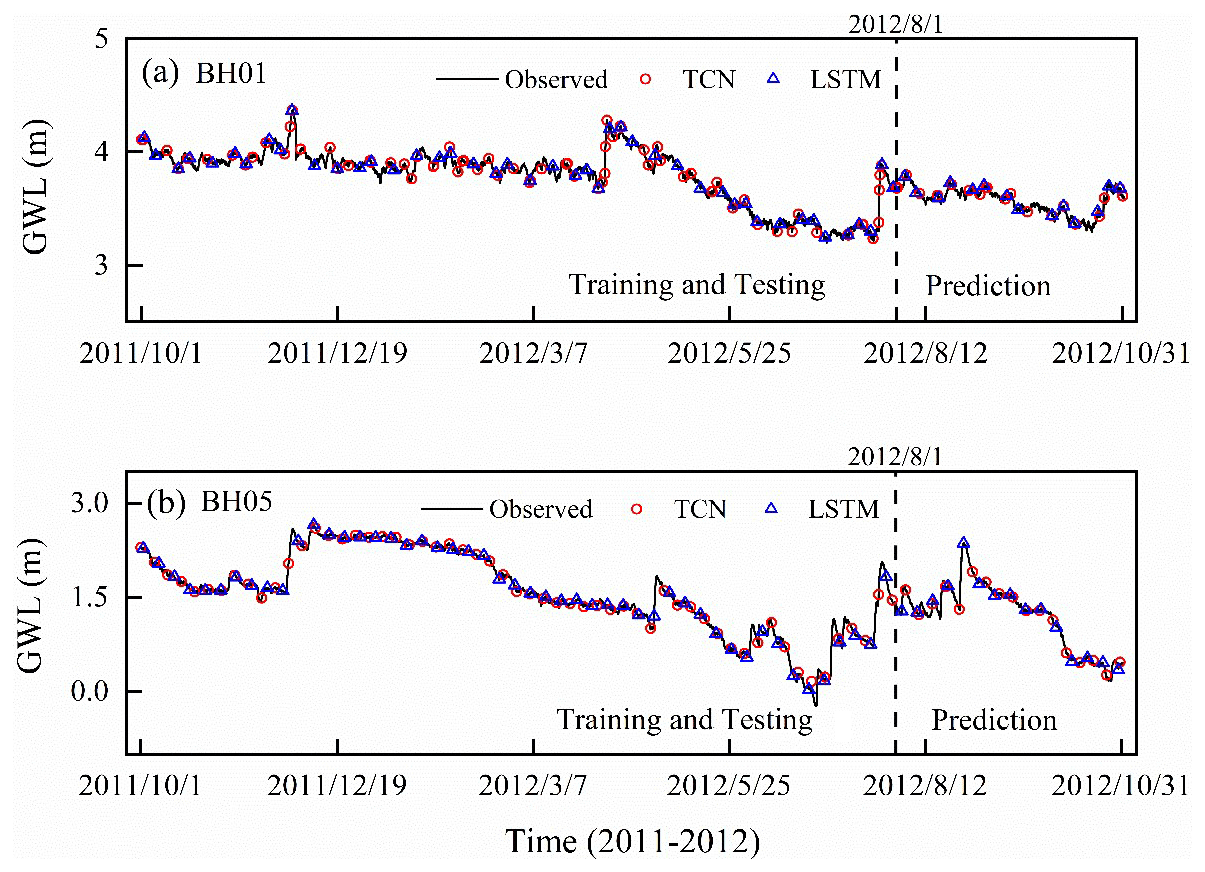
Figure 7 The simulation results of groundwater level of monitoring wells BH01 and BH05 by TCN-based model. The dashed black line divides the data into two groups: the training and testing dataset, and the prediction dataset.

Table 3 The model results for groundwater level in the training and testing and prediction stage.

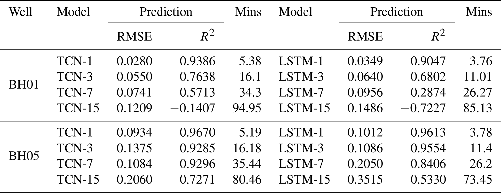
Table 4 The model results for groundwater level in the long-term prediction.

4.3 Long-term leading time prediction

The TCN- and LSTM-based models were further adjusted to predict the groundwater levels over 3 months ahead with different leading periods. Prediction results with 1, 3, 7, and 15 d leading time with TCN- and LSTM-based models are illustrated in Figs. 8 and 9 for wells BH01 and BH05, respectively. The results show that the predicted groundwater values have the same change trend as the actual groundwater level in monitoring wells. Both of the models are able to capture the variation trend of groundwater levels with longer leading periods of more than 1 time step in the two monitoring wells.

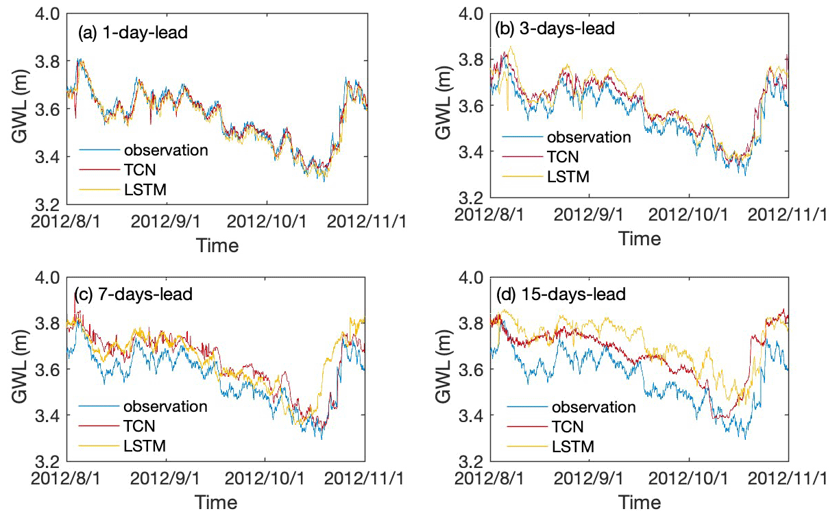
Figure 8 The observed and predicted values of the groundwater level with TCN- and LSTM-based models for 1, 3, 7, and 15 d lead period in monitoring well BH01.

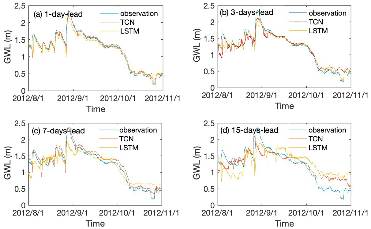
Figure 9 The observed and predicted values of the groundwater level with TCN- and LSTM-based models for 1, 3, 7, and 15 d leading period in monitoring well BH05.

To quantitatively compare the prediction accuracy of the proposed TCN- and LSTM-based models, the results of two evaluation metrics with the model running time are summarized in Table 4. It can be learned that the R² value of TCN-based models decreased from 0.9386 to −0.1407 for well BH01 and from 0.9670 to 0.7271 for well BH05. Correspondingly, an increase in RMSE values from 0.028 to 0.1209 and 0.0934 to 0.206 are observed for BH01 and BH05, separately. A similar variation pattern is recognized for the LSTM-based model with smaller R² and higher RMSE than that of the TCN-based model. Notably, the running time of advance prediction is much longer than that of a single-step prediction. Meanwhile, with the increasing leading period, the time had been raised nonlinearly. Further, in this process, the TCN-based model costs longer time than that of the LSTM-based model.

The performance of the two networks was further evaluated with Taylor diagrams by taking different criteria aspects, including standard deviation (SD), correlation coefficient (COR), and root mean square deviation (RMSD) into account (Taylor, 2001). The comparisons of the TCN- and LSTM-based models are shown in Fig. 10. As the metrics are distributed away from the reference point (Ref), the deviation of prediction from observation is generally increased with extending the leading period. Taking well BH05 as an example, the prediction with 1 d (24 h prediction window) in advance is the highest in agreement with the actual situation in the two models. The 1 d leading prediction results have the lowest RMSD values and highest R² values for both models. The prediction precision gradually decreases with the extension of leading time to 3, 7, and 15 d. For well BH01, an out-of-trending point is observed. The 15 d prediction results of the LSTM-based model are closer to the Ref point compared with the TCN-based model. The reason is that the simulation data are highly correlated with observations as shown in Fig. 8.

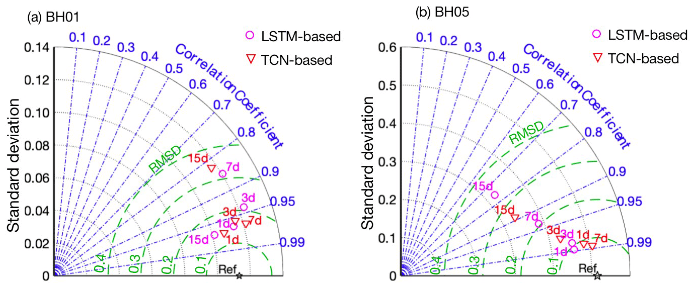
Figure 10 Taylor diagrams with statistical (SD, COR, RMSD) comparison results of the TCN-based and LSTM-based models for well (a) BH01, (b) BH05.

Overall, the TCN- and LSTM-based models both have strong prediction abilities in long-term hydrological time-series data. Both models are able to provide accurate predictions once they are trained. The simulation accuracy of the TCN-based model is slightly better than that of the LSTM-based model in the 3 months prediction, but the difference is not significant with p>0.05 in the t test. The causal dilated convolutions used by TCNs are proven to be good at capturing long-term dependencies of time-series data. Meanwhile, the model precision decreases and the running time increases with the raising leading period. The processing speed of parallel convolution TCN-based models for long input sequences is slower than that of recurrent networks. This seems to be a shortage in real-time monitoring and early warning. A leading period shorter than 7 d is recommended to ensure both the accuracy and efficiency of the models in real-time monitoring and early warning.

From the groundwater-level variation, significant groundwater decreasing trends can be observed in the irrigation season from March to June. Therefore, human activities, such as groundwater pumping are potential reasons for groundwater-level change in the study area. Here, the groundwater levels were predicted based on the available data of precipitation and tide. If the pumping data are available and considered in the models, the prediction precision would be enhanced in the models.

4.4 Influence of training set percentage

The data-driven methods are supported by data; however, how much data are needed to build an effective model is still a challenging problem (Reichstein et al., 2019). This is because specific problems depend on application cases, data features, and model features (Wunsch et al., 2021). Here, we discuss the effect of the training set percentage on the TCN- and LSTM-based models. In our study, the data are the data from 2011 to 2012 that were monitored hourly. From 2011, we set 20 % to 90 % training sets in turn, so as to gradually expand the length of the training set.

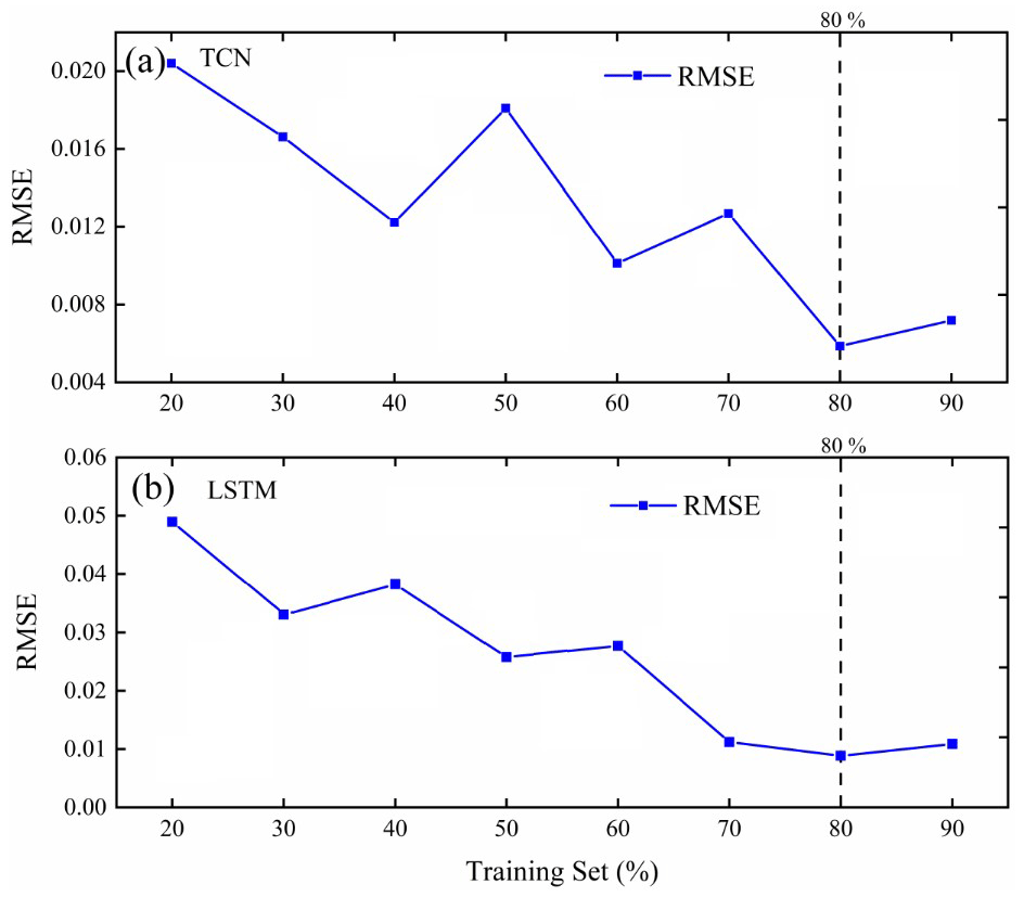
Figure 11 Influence of training set percentage on the performance of the model for (a) BH01 and (b) BH05.

Figure 11 shows the effect of the increased percentage of the training set on the performance of the model. All experiments were repeated five times, and the average values of each index were compared. It can be seen that the performance of the TCN-based model varied with the increase in the percentage of the training set. When the training set reached 80 %, the performance was relatively optimal. At the same time, it can be seen that the performance of the LSTM-based model tends to be stable when the training set reaches 80 % as well. Therefore, a training set evaluation is recommended before the training and testing. We should carefully evaluate and shorten the training dataset as much as possible when necessary. Finally, we set 80 % of the training set length to simulate the coastal aquifer time-series data.

5 Conclusions

The TCN- and LSTM-based deep-learning models were proposed in this paper to predict groundwater levels in a coastal aquifer. Hyper-parameter searches were first conducted to obtain good architecture configurations. The results indicated that a deeper, broader model does not necessarily guarantee better predictions. The optimal configurations were then adopted for the networks of all monitoring data. Both the TCN- and LSTM- based models well captured the fluctuation of groundwater levels and achieved satisfactory performance on the prediction. Meanwhile, a decreasing precision is revealed when the leading time increases in advance prediction. In view of accuracy, the TCN-based model outperforms the LSTM-based model but is less efficient in long-term simulation. Thus, both models can be used as a promising method for time-series prediction of hydrogeological data, especially when the regional data are difficult to collect in a complex system.