the Creative Commons Attribution 4.0 License.
the Creative Commons Attribution 4.0 License.
 | 20 Dec 2023
Comparing quantile regression forest and mixture density long short-term memory models for probabilistic post-processing of satellite precipitation-driven streamflow simulations
Yuhang Zhang
Bita Analui
Phu Nguyen
Soroosh Sorooshian
Kuolin Hsu
Yuxuan Wang
Deep learning (DL) and machine learning (ML) are widely used in hydrological modelling, which plays a critical role in improving the accuracy of hydrological predictions. However, the trade-off between model performance and computational cost has always been a challenge for hydrologists when selecting a suitable model, particularly for probabilistic post-processing with large ensemble members. This study aims to systematically compare the quantile regression forest (QRF) model and countable mixtures of asymmetric Laplacians long short-term memory (CMAL-LSTM) model as hydrological probabilistic post-processors. Specifically, we evaluate their ability in dealing with biased streamflow simulations driven by three satellite precipitation products across 522 nested sub-basins of the Yalong River basin in China. Model performance is comprehensively assessed using a series of scoring metrics from both probabilistic and deterministic perspectives. Our results show that the QRF model and the CMAL-LSTM model are comparable in terms of probabilistic prediction, and their performances are closely related to the flow accumulation area (FAA) of the sub-basin. The QRF model outperforms the CMAL-LSTM model in most sub-basins with smaller FAA, while the CMAL-LSTM model has an undebatable advantage in sub-basins with FAA larger than 60 000 km2 in the Yalong River basin. In terms of deterministic predictions, the CMAL-LSTM model is preferred, especially when the raw streamflow is poorly simulated and used as input. However, setting aside the differences in model performance, the QRF model with 100-member quantiles demonstrates a noteworthy advantage by exhibiting a 50 % reduction in computation time compared to the CMAL-LSTM model with the same ensemble members in all experiments. As a result, this study provides insights into model selection in hydrological post-processing and the trade-offs between model performance and computational efficiency. The findings highlight the importance of considering the specific application scenario, such as the catchment size and the required accuracy level, when selecting a suitable model for hydrological post-processing.
- Article
(5542 KB) - Full-text XML
-
Supplement
(1953 KB) - BibTeX
- EndNote


By generalizing the physical processes, hydrologists or modellers abstract the hydrological mechanism into a series of numerical equations, collectively known as hydrological models (Sittner et al., 1969; Clark et al., 2015; Sivapalan, 2018; Chawanda et al., 2020; Zhou et al., 2021). Hydrological models are widely used for rainfall-runoff simulation, flood forecasting, drought assessment, decision-making, and water resource management (Corzo Perez et al., 2011; Tan et al., 2020; Wu et al., 2020; Gou et al., 2020, 2021; Miao et al., 2022). Depending on the complexity, hydrological models can be classified as lumped, semi-distributed, and distributed models (Beven, 1989; Jajarmizadeh et al., 2012; Khakbaz et al., 2012; Mai et al., 2022a, b). Although current models simulate the hydrological processes well, they still suffer from multiple uncertainties, including input uncertainty, model structure and parameter uncertainty, and observation uncertainty (Nearing et al., 2016; Herrera et al., 2022). These uncertainties limit the accuracy of hydrological models (Honti et al., 2014; Sordo-Ward et al., 2016; Mai et al., 2022a, b). Among these various sources, input uncertainty is considered one of the largest sources of uncertainty. Hence, precipitation, which is the driver of the water cycle, is the most important factor affecting streamflow simulation (Kobold and Sušelj, 2005).
Precipitation information is mainly derived from gauge observations, radar estimates, satellite retrievals, and reanalysis products (Sun et al., 2018). Gauge stations and radars are limited by the density of their network and by topography, especially in remote areas such as mountainous regions and high altitudes (Sun et al., 2018; Chen et al., 2020). Reanalysis requires assimilation of the observations from multiple sources and therefore cannot be obtained in real time. Satellite precipitation estimates are available in near-real time and have shown valuable potential for applications in regions where ground measurements are scarce (Jiang and Bauer-Gottwein, 2019; Dembélé et al., 2020). Over the past decades, several research institutions have developed various satellite precipitation estimation products with different data sources and algorithms: for example, the Integrated Multi-satellitE Retrievals for Global Precipitation Measurement Mission (GPM IMERG) products jointly developed by the National Aeronautics and Space Administration (NASA) and the Japan Aerospace Exploration Agency (JAXA) (Hou et al., 2013; Huffman et al., 2020); the Global Satellite Mapping of Precipitation (GSMaP) products developed by JAXA (Kubota et al., 2007, 2020); and the Precipitation Estimation from Remotely Sensed Information using Artificial Neural Networks-Dynamic Infrared Rain Rate (PDIR-Now, hereafter PDIR) near-real-time product developed by the Centre for Hydrometeorology and Remote Sensing (CHRS) at the University of California, Irvine (UCI) (Nguyen et al., 2020a, b). However, uncertainties persist in these products due to various factors, including data sources and algorithms. Additionally, the coarse resolution still limits their use for small basins, i.e. those with an area smaller than 200 km2 (Tian et al., 2009; Zhang et al., 2021a). Moreover, these uncertainties are further propagated during the hydrological simulation (Cunha et al., 2012; Falck et al., 2015; Zhang et al., 2021b), significantly restricting their effectiveness in downstream hydrological applications.
Satellite precipitation introduces notable uncertainties in hydrological modelling. Various strategies, such as meteorological pre-processing and hydrological post-processing, have emerged to address this challenge (Schaake et al., 2007; Wang et al., 2009; Ye et al., 2014, 2015; Li et al., 2017; Dong et al., 2020; Shen et al., 2021; Zhang et al., 2022a). Meteorological pre-processing predominantly focuses on achieving bias-corrected precipitation estimates. This is often realized by fusing satellite precipitation data with ground observations to mitigate input uncertainty (Xu et al., 2020; Zhang et al., 2022a). Conversely, hydrological post-processing leverages observed streamflow to rectify simulations or predictions, providing an additional layer of refinement, especially if the meteorological pre-processing stage falls short. Both these strategies can be employed for deterministic and probabilistic predictions (Ye et al., 2014; Tyralis et al., 2019). Given the inherent autocorrelation in streamflow time series, two main methods stand out for hydrological post-processing. The first method employs autoregressive models anchored on residuals, using these residuals as predictors to adjust forecast errors (Li et al., 2015, 2016; Zhang et al., 2018). The second method employs the model output statistics (MOS) concept, leveraging simulated streamflow as a primary predictor to establish statistical relationships between simulations and observations (Wang et al., 2009; Bogner and Pappenberger, 2011; Zhao et al., 2011; Bellier et al., 2018).
In recent years, machine learning (ML) and deep learning (DL) algorithms have emerged as powerful tools in hydrological modelling (Sit et al., 2020; Zounemat-Kermani et al., 2021; Shen and Lawson, 2021; Fang et al., 2022). ML comprises a broad range of algorithms, with commonly used models such as random forest, support vector machines, and clustering methods. DL, a specialized subset of ML, emphasizes algorithms modelled on the architecture of artificial neural networks, including models like convolutional neural networks, recurrent neural networks, and long short-term memory networks. In this study, we use the term “ML models” to refer to non-DL models while specifically designating “DL models” to refer to models based on deep learning techniques. In the hydrological field, both random forest (RF) and long short-term memory (LSTM) models are widely used and considered state-of-the-art approaches for various tasks and applications. The RF model and its probabilistic variant, the QRF model, have demonstrated capabilities in bias correction and streamflow simulation (Shen et al, 2022; Tyralis et al., 2019; Zhang and Ye, 2021). For example, Shen et al. (2022) used the RF model as a hydrological post-processor to enhance the simulation performance of the large-scale hydrological model PCR-GLOBAL (PCRaster Global Water Balance) model at three hydrological stations in the Rhine basin. Tyralis et al. (2019) compared the usability of the statistical model (e.g. quantile regression) and the machine learning algorithm (e.g. quantile regression forests) as hydrological post-processors on the CAMELS (Catchment Attributes and Meteorology for Large-sample Studies) dataset. And the results showed that the quantile regression forest model outperformed the quantile regression. In the context of bias correction applications, RF models have also exhibited superior performance compared to other machine models (Zhang and Ye, 2021). The LSTM model, on the other hand, has gained widespread recognition as leading choice in hydrological applications (Kratzert et al., 2018, 2019). For example, LSTM models have been used to simulate streamflow in a number of gauged and ungauged basins in North America (Kratzert et al., 2018, 2019), the United Kingdom (Lees et al., 2021), and Europe (Nasreen et al., 2022). Frame et al. (2021) utilized the LSTM model to develop a post-processor that can effectively improve the accuracy of the US National Hydrologic Model. They validated the performance of the proposed post-processor on the CAMELS dataset, which consists of 531 watersheds across North America. By integrating with Gaussian models (Zhu et al., 2020), stochastic deactivation of neurons (Althoff et al., 2021), and Bayesian perspective (Li et al., 2021, 2022), LSTM further solidified its reputation for delivering reliable probabilistic predictions. More recently, Klotz et al. (2022) compared the use of dropout and three Gaussian mixture density models for uncertainty estimation in LSTM rainfall-runoff modelling. They found that the mixture density model outperformed the random dropout model and provided more reliable probabilistic information.
While both RF and LSTM models have seen significant advancements and widespread application, a thorough comparative analysis specifically within the context of hydrological probabilistic post-processing is yet to be undertaken. Through their hierarchical feature learning, DL models, especially LSTM models, can autonomously extract insights from raw hydrological data, capturing long-term dependencies and patterns without extensive feature engineering. In contrast, with ML models like RF, effort is often required to select relevant features to adequately represent the data. Additionally, DL models can effectively leverage massive datasets, leading to enhanced generalization and improved accuracy in hydrological prediction tasks. On the other hand, ML models may face limitations in capturing intricate patterns from large hydrological datasets. Notwithstanding pieces of evidence, it is essential to conduct a direct and focused comparison between RF and LSTM models in the specific context of hydrological probabilistic post-processing to better understand their respective strengths and limitations, such as the scope of application, model performance and computational efficiency.
Hydrological probabilistic post-processing represents a big-data task with the involvement of large datasets and a substantial number of ensemble members. The complex relationships between input and output variables in hydrological systems necessitate advanced modelling techniques to achieve accurate and reliable predictions. Therefore, in this study, we attempt to comprehensively compare the performance of the two most widely used ML and DL models for streamflow probabilistic post-processing, quantile regression forests (QRF) and countable mixtures of asymmetric Laplacians LSTM (CMAL-LSTM), at a sub-basin scale daily streamflow, respectively. In particular, a full model comparison is performed in a complex basin with 522 nested sub-basins in southwest China. Three sets of global satellite precipitation products are applied to generate uncorrected streamflow simulations. The three precipitation products represent different algorithms. Also, they have been proven to have relatively good accuracy in our previous study (Zhang et al., 2021b). These satellite precipitation products are compared across two scenarios, single-product and multi-product simulations, both used as input features for streamflow post-processing. A variety of evaluation metrics are used to assess the performance of the proposed models, including probabilistic metrics for multi-point prediction and deterministic metrics for single-point prediction. Additionally, the study also analyses the relationship between model performance and basin size by considering the disparity in the flow accumulation area of the sub-basins. Through a comparative analysis of QRF and CMAL-LSTM models in hydrological probabilistic post-processing, this study aims to provide clarity on their respective merits and drawbacks. The insights garnered will also guide the selection of other ML and DL methodologies with similar model architectures.
The rest of paper is organized as follows: in Sect. 2, we introduce the study area and data. In Sect. 3, we present the post-processing models, experimental design, and evaluation metrics. Section 4 presents the streamflow results before and after post-processing with different experiments. In Sect. 5, we discuss the interpretation of post-processing model differences, as well as their limitations. Finally, the conclusions are summarized at the end of this article.
2.1 Study area
The Yalong River (Fig. 1a) is a major tributary of the Jinsha River, which belongs to the upper reaches of the Yangtze River. The Yalong River basin is located between the Qinghai–Tibet Plateau and the Sichuan Basin. The Yalong River basin has a long and narrow shape (26∘32′–33∘58′ N, 96∘52′–102∘48′ E); it has snow-capped mountains scattered in the upper reaches, it is surrounded by high mountain valleys in the middle reaches, and it flows into the Jinsha River in the lower reaches. It spans seven dimensional zones with complex climate types. The total length of the basin is about 1570 km, and the total area is about 130 000 km2. The mean annual precipitation of the basin is about 800 mm.

Figure 1(a) Study area and (b) 522 sub-basins (Zhang et al., 2022a).
Following the watershed division method of Du et al. (2017), Yalong River basin is divided into 522 nested sub-basins with catchment areas ranging from 100 to 127 164 km2 (Fig. 1b). The key to sub-basin delineation is the minimum catchment area threshold (100 km2 in this study), which is related to the total area of the basin, the model architecture complexity, the step size, and the spatial resolution of the input data. The location, elevation, area, flow accumulation area, and flow direction of each sub-basin can be found in Table S1 in the Supplement.
2.2 Data
2.2.1 Gauge precipitation observations
The 0.5∘ daily precipitation observation data were obtained from the National Meteorological Information Centre of the China Meteorological Administration (CMA-NMIC). The product was produced by interpolating gauge data from more than 2000 stations across China. This product has been proven to be highly accurate and has been widely applied to a variety of studies such as streamflow simulation, drought assessment, and water resource management (Gou et al., 2020, 2021; Zhang and Ye, 2021; Miao et al., 2022). In this study, the gridded precipitation observations are used as a reference for the satellite-based precipitation products. Using the inverse distance weighting (IDW) method, the gridded precipitation observations are resampled to each sub-basin. This resampling process aims to obtain the sub-basin average precipitation amount, which serves as the forcing input for hydrological simulations. Errors caused by resampling are ignored. And due to limited hydrological stations, the streamflow of each sub-basin obtained from the calibrated hydrological model driven by this product is also used as a reference for the satellite precipitation-driven streamflow simulations. The selected study period is from 1 January 2003 to 31 December 2018.
2.2.2 Global satellite precipitation estimates
Three sets of the latest quasi-global satellite precipitation estimation products are selected. The first one is the PDIR product, which solely relies on infrared data. It has a very high spatiotemporal resolution (0.04∘ and 1 h) and a very short delay time (1 h). The other two products are bias-adjusted products, IMERG Final Run version 6 (hereafter IMERG-F) (Huffman et al., 2019, 2020) and the Gauge-calibrated GSMaP product (GSMaP_Gauge_NRT_v6; hereafter GSMaP) (Kubota et al., 2007, 2020), with a spatial resolution of 0.1∘. The selected study period is also from 1 January 2003 to 31 December 2018. All these products are aggregated to the daily scale and resampled to each sub-basin using IDW. It should be noted that these products are selected as examples only, and any other precipitation product can be used as an alternative.
2.2.3 Other data
In addition to precipitation gauge observations and satellite precipitation products, hydrological modelling requires other meteorological data such as temperature, wind speed, and evaporation. The meteorological data were also obtained from the CMA-NMIC and were used to drive the hydrological model together with precipitation. In addition, watershed attributes, including elevation, soils, and land use, are also important parts of accurate hydrologic modelling. The National Aeronautics and Space Administration Shuttle Radar Topographic Mission (NASA SRTM) digital elevation model (DEM) data with a spatial resolution of 90 m were obtained from the Geospatial Data Cloud of China. The 1 km soil data were clipped from the China Soil Database issued by the Tibetan Plateau Data Centre of China. The 1 km land use data were obtained from the Resource and Environment Science and Data Centre provided by the Institute of Geographical Sciences and Resources, Chinese Academy of Sciences. Finally, streamflow observations are used to calibrate and validate the hydrologic model. The streamflow observations (1 January 2006 to 31 December 2015) were collected from four gauged hydrological stations in the Yalong River basin from the upstream to the downstream, namely Ganzi (GZ), Daofu (DF), Yajiang (YJ), and Tongzilin (TZL) (Fig. 1a). And they were obtained from the Hydrological Yearbook of the Bureau of Hydrology.
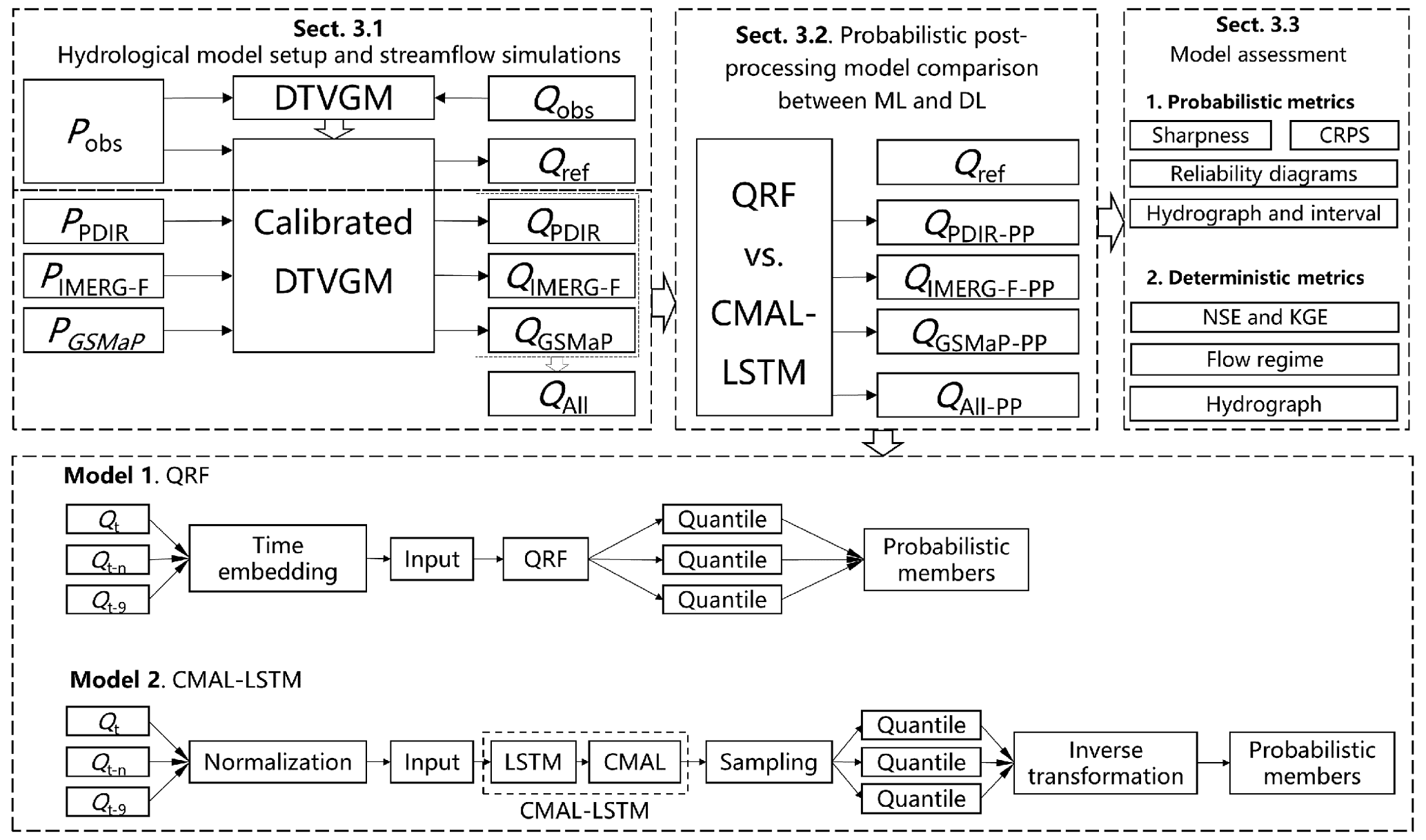
The framework of this study is shown in Fig. 2. We adopt a two-stage streamflow post-processing approach. In the first stage (Sect. 3.1), the hydrological model is calibrated and validated by hydrological station observations. Then, we use the observed precipitation to drive the calibrated hydrological model to generate streamflow references for each sub-basin. And we use satellite precipitation to drive the model to generate uncorrected (raw) streamflow simulations. In the second stage (Sect. 3.2), we perform probabilistic post-processing of the streamflow using the QRF and the CMAL-LSTM models. In the last subsection (Sect. 3.3), we describe the evaluation metrics that are used in this study.
3.1 Streamflow reference and uncorrected streamflow simulations
The purpose of this study is to post-process the streamflow simulations for all sub-basin outlets, and therefore corresponding references are needed. Due to the limited streamflow observations, we use streamflow simulations from the hydrological model driven by observed precipitation as a reference. To ensure that the results are reliable, we first use the collected streamflow observations from four hydrological stations to set up, calibrate, and validate the hydrological model.
We choose the distributed time-variant gain model (DTVGM), a process-based hydrological model that uses the rainfall-runoff nonlinear relationship (Xia, 1991; Xia et al., 2005) for simulation. In each sub-basin, runoff is calculated according to Eq. (1).
where t is the time step; P, E, and EP are precipitation, actual evapotranspiration, and potential evapotranspiration, respectively; Rs, Rsoil, and Rg are surface runoff, interflow runoff, and groundwater runoff, respectively; AW and WM are soil moisture (mm) and field soil moisture (mm), respectively; u and g are the upper and lower soil layers, respectively; Ke, Kr, and Kg are evapotranspiration, interflow, and groundwater runoff coefficients, respectively; g1 and g2 are factors describing the non-linear rainfall-runoff relationship; and C is the land cover parameter.
The kinematic wave equation is used for river routing (Ye et al., 2013). The snowmelt process in the high-altitude regions of the basin is simulated by the degree-day method (Bormann et al., 2014). A detailed description of the DTVGM model can be found in Xia et al. (2005) and Ye et al. (2010).
Based on the length of the streamflow observation collected from hydrological stations (2006–2014), we divide the streamflow time series into three periods: a 1-year spin-up period (2006), a 4-year calibration period (2007–2010), and a 4-year validation period (2011–2014). We use the Nash–Sutcliffe efficiency (NSE) as the objective and regionalize the parameters from upstream to downstream using manual tuning, while ensuring that the water balance coefficient (the ratio of simulated streamflow to observed streamflow) converges to 1. Specifically, the regional parameters are evaluated and adjusted sequentially, moving from upstream to downstream of the hydrological stations. Initially, the regional parameters are fixed in the upstream station, ensuring their consistency throughout the region. Then, the focus shifts to adjusting the regional parameters between the upstream and downstream stations. This sequential process continues until the parameter regionalization is completed across all four stations. The model calibration and validation are shown in Fig. S1 in the Supplement. The NSEs for the four gauged hydrological stations (GZ, DF, YJ, and TZL) are 0.89, 0.91, 0.93, and 0.79 and 0.79, 0.86, 0.87, and 0.59 for calibration and validation periods, respectively. In the remaining part of this study, the hydrological model is fixed, and we mainly post-process the streamflow bias introduced by satellite precipitation, disregarding other sources of uncertainty such as model structure, DEM, and other forcing data.
After model calibration and validation, to ensure the number of data samples for data-driven post-processing methods, we use the observed precipitation from 2003 to 2018 to drive the hydrological model. A 16-year streamflow simulation reference dataset is obtained for 522 sub-basin outlets. Streamflow from different sub-basins can also reflect hydrological processes of diverse climate types and scales.
In the final step, we utilize the three satellite precipitation products, namely PDIR, IMERG-F, and GSMaP, to drive the hydrological model over the period of 2003–2018. As a result, three raw simulations, PDIR-driven, IMERG-F-driven, and GSMaP-driven, are generated. Furthermore, the equally weighted average of these three raw simulations can be regarded as a multi-product-driven simulation referred to as “All” in the following sections of this study. There are two main reasons for considering the multi-product simulation (All) as a reference. The first reason for considering “All” as a reference is to allow for a comprehensive comparison of the model performance of the two post-processing models in different contexts, utilizing multiple input scenarios. This robust assessment evaluates the capabilities of the models across various satellite precipitation products. The second reason is to examine the effects of the model averaging method and the multi-dimensional features on the post-processing models. By comparing the models' performance with multiple inputs, the study assesses the impact of incorporating different sources of information and the potential benefits of using a combination of satellite precipitation products. The experimental design is described in Sect. 3.2.
3.2 Post-processing model and experimental design
The two post-processing models selected are the QRF model (Meinshausen and Ridgeway, 2006) and the CMAL-LSTM model (Klotz et al., 2022). The QRF model was chosen because it enables us to analyse the distribution of the entire data based on different quantiles, and it has been previously used in several studies (Taillardat et al., 2016; Evin et al., 2021; Kasraei et al., 2021; Tyralis et al., 2019; Tyralis and Papacharalampous, 2021). The CMAL-LSTM model is a combination of an LSTM model and a CMAL mixture density function, which allows it to provide information about prediction uncertainties. To the best of our knowledge, these two models are currently considered state-of-the-art approaches in ML and DL for hydrological probabilistic modelling (Tyralis et al., 2019; Zhang and Ye, 2021; Klotz et al., 2022). Readers who wish to delve into more comprehensive details about each mentioned model are strongly encouraged to refer to the original papers.
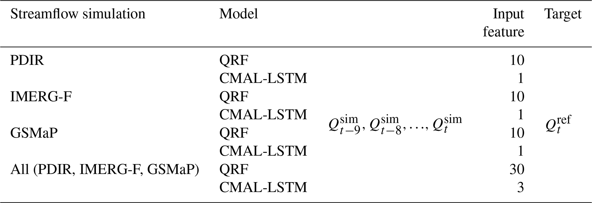
To manage the complexity of the models, only the uncorrected (raw) streamflow simulations are chosen as input features. Based on the autocorrelation characteristic of the streamflow, as depicted in Fig. S2, the post-processing for day t(Qt) involves selecting the simulated streamflow for the previous 9 d (, , …, ) as well as the simulated streamflow for the current day () as inputs. In the QRF model, the input features are fed by temporal embedding. And in the CMAL-LSTM model, the sequence length is set to 9. For both models, we select the streamflow reference () on day t as the target. In addition, since we used three different satellite precipitation products, the experiments are divided into a single-product experiment and a multi-product experiment (All). The information for each experiment is summarized in Table 1. The training period is from 1 January 2003 to 31 December 2010. The validation period is from 1 January 2011 to 31 December 2014. And the test period is from 1 January 2015 to 31 December 2018.
We implemented the QRF model using the pyquantrf package (Jnelson18, 2022). We tuned three sensitive hyperparameters in the QRF model by grid search, finally setting the number of trees (K) to 70, the number of non-leaf node splitting features to 10, and the number of samples used for leaf node predictions (Nleaf) to 10. All other hyperparameters were set to default values.
We implemented the CMAL-LSTM model using the NeuralHydrology package (Kratzert et al., 2022a). We followed the model architecture of Klotz et al. (2022), which contains an LSTM layer and a CMAL layer. In contrast to the QRF model, the input data of the CMAL-LSTM model need to be normalized. Here, through several comparisons, we used the normal quantile transform method (Fig. S3). The hyperparameters of the model include the number of neurons in the LSTM layer (NLSTM), the number of components of the mixture density function (NMDN), the dropout rate, the learning rate, the epoch, and the batch size. NMDN, is set to 3, which follows Klotz et al. (2022). The other hyperparameters are also fine-tuned such that the final learning rate is set to 0.0001, the dropout to 0.4, the epoch to 100, the batch size to 256, and the NLSTM to 256.
For the QRF model, 100 percentiles (0.005 to 0.995) were equally sampled for each basin and time step and fed directly into the model to obtain the final probabilistic (100) members. For the CMAL-LSTM model, first, 10 000 sample points for each basin and time step by sampling from the mixture distribution were generated, and the same 100 percentiles (0.005 to 0.995) from these sample points were extracted and remapped to the original streamflow space using inverse quantile normal transformation, where finally the probabilistic members were produced.
Our computing platform is a workstation configured with an Intel(R) Xeon(R) Gold 6226R CPU @ 2.9 GHz and an RTX3090 GPU with 24 GB video memory. It is important to note that each sub-basin was modelled separately due to the GPU's video memory limitation in the random sampling process of the CMAL-LSTM model. For consistency, the QRF model was also modelled locally. The computational time was approximately 12 h to complete all CMAL-LSTM and 6 h to complete all QRF experiments.
3.3 Performance evaluation
In this section the two post-processing models are evaluated from both probabilistic and deterministic perspectives. These evaluation metrics are presented in Sect. 3.3.1 and 3.3.2, respectively.
3.3.1 Probabilistic (multi-point) metrics
We followed the criterion for probabilistic predictions proposed by Gneiting et al. (2007), and the aim is to maximize the sharpness of the prediction distributions subject to reliability. We use both scoring rules and diagnostic graphs to assess reliability and sharpness holistically.
The continuous rank probability score (CRPS) is a widely used scoring measure that assesses reliability and sharpness simultaneously (Gneiting et al., 2007; Bröcker et al., 2012). For given probabilistic prediction members, the CRPS calculates the difference between the cumulative distribution function (CDF) of the probabilistic prediction members and the observations. We also used a weighted version of CRPS (threshold-weighted CRPS, twCRPS), which is commonly used to give more weight to extreme cases (Gneiting and Ranjan, 2011). These two metrics can be expressed as follows:
where ω(y) is a threshold-weighted function and is calculated based on the threshold q (80 %, 90 % and 95 % percentiles of observations in this study). When y≥q (y < q), ω(y) equals 1 (0). x represents the observations, i.e. the streamflow reference. F(y) is the CDF obtained from the probabilistic members for the corrected streamflow. 1(y≥x) is the Heaviside step function. The better-performing model has both metrics (CRPS and twCRPS) closer to 0.
The CRPS skill score (CRPSS) is also used to define the relative differences between the two post-processing models. For QRF and CMAL-LSTM, the CRPSS can be calculated as
A CRPSS greater than 0 indicates that the QRF model is better than the CMAL-LSTM model, and vice versa.
The reliability diagram serves as a diagnostic graph to assess the agreement between predicted probabilities and observed frequencies (Jolliffe and Stephenson, 2012). It plots the observed frequencies of events against the predicted probabilities, specifically plotting the cumulative distribution function (CDF) of the streamflow reference as a function of the forecasted probability. The diagram helps to evaluate the reliability of probabilistic forecasts by comparing the predicted probabilities of events with their corresponding observed relative frequencies. Ideally, in a perfectly reliable forecast, if the predicted probability of a specific event is, for example, 30 %, then the observed relative frequency of that event should also be around 30 %. Consequently, the reliability diagram would show a distribution of points lying along the diagonal line, indicating a consistent alignment between predicted probabilities and observed frequencies across various probability levels. However, in practice, there may be deviations from perfect reliability. Points on the reliability diagram above the diagonal line suggest that the observed relative frequency is higher than the predicted probability, indicating an underprediction phenomenon. On the other hand, points below the diagonal line indicate that the observed relative frequency is lower than the predicted probability, indicating an overprediction phenomenon. Here again, three thresholds (80 %, 90 %, and 95 %) are chosen to better evaluate the reliability of extreme cases (Yang et al., 2021).
Sharpness refers to the precision or tightness of a probabilistic prediction, capturing how closely the predicted probability distributions align with the observations. Essentially, a sharp forecast indicates that the predicted uncertainties are relatively narrow and closely resemble the observed data points, reflecting a more accurate representation of the true uncertainty in the predictions. A sharp probabilistic output corresponds to a low degree of variability in the predictive distribution. To evaluate the sharpness of probabilistic predictions, prediction intervals are commonly employed (Gneiting et al., 2007). For this study, the 50 % and 90 % percentile intervals were chosen. Furthermore, to establish the relationships between predictive distributions and observations, we assessed the coverage of the prediction intervals over the observations. The average Euclidean distance of the 25 % and 75 % probabilistic members is adopted as the sharpness metric (DIS25–75) for the 50 % prediction interval, and the 5 % and 95 % probabilistic members were used to compute the sharpness metric (DIS5–95) for the 90 % prediction intervals. The ratio of the number of observations in the prediction intervals to the total number of observations was used as the coverage of observations (CO25–75 and CO5–95). In addition, three additional metrics used in a previous study (Klotz et al., 2022) are also employed to calculate the sharpness metric for the full probabilistic members, including mean absolute deviation (MAD), standard deviation (SD), and variance (VAR).
3.3.2 Deterministic (single-point) metrics
The widely used Nash–Sutcliffe efficiency (NSE) (Nash and Sutcliffe, 1970) and Kling–Gupta efficiency (KGE) (Gupta et al., 2009; Kling et al., 2012) are applied for assessing the deterministic model performance. In addition, two components of the NSE, namely Pearson correlation coefficient (PCC) and relative bias (RB) are calculated to assess the temporal consistency and systematic bias of the difference between simulations and observations, respectively. Furthermore, to account for the seasonality of the flow regime, four metrics are selected to characterize the different aspects of flow regimes, including the peak flow bias (FHV; Eq. A3 in Yilmaz et al., 2008), low-flow bias (FLV, Eq. A4 in Yilmaz et al., 2008), flow duration curve bias (FMS; Eq. A2 in Yilmaz et al., 2008), and mean peak time lag bias (in days) (PT; Appendix D in Kratzert et al., 2021). These metrics provide a comprehensive assessment of model performance across different flow conditions and facilitate a more accurate evaluation of model ability to reproduce the hydrological processes.
4.1 Uncorrected streamflow simulations
Figure 3 shows the spatial distribution of NSEs for streamflow simulations in 522 sub-basins, driven by three different satellite precipitation products and multi-product outputs using the equally weighted averaging (All). Among the three satellite precipitation products, IMERG-F achieves the best model performance, followed by PDIR and GSMaP. PDIR performs poorly in the upstream and outlet regions of the basin. GSMaP exhibits significant deviations from the streamflow reference in almost all sub-basins. The quality of that precipitation product plays a crucial role in streamflow performance with the same hydrological model configuration. For example, the presence of a high precipitation bias in GSMaP, as observed in Fig. S4f, has significant implications for streamflow simulations. This bias leads to correspondingly high biases in the streamflow simulations, as depicted in Fig. 8b. Consequently, the streamflow simulations driven by GSMaP exhibit the lowest NSE values among the three products, as shown in Figs. 3c and 8c. The performance of PDIR-driven streamflow is mainly influenced by the poor temporal variability (PCC) against observations (Figs. S4a and 8a). Equally weighted averaging (All) that incorporates biased information from PDIR and GSMaP has an insignificant impact on improving model performance.

Figure 3The NSE of uncorrected streamflow simulation for the 522 sub-basins.
4.2 Probabilistic (multi-point) assessment
The flow magnitudes in different sub-basins vary widely. Therefore, in the presented results for each sub-basin, the results are normalized separately according to the probabilistic membership of all experiments. By doing so, the probabilistic members of all sub-basins are mapped to the range between 0 and 1.
4.2.1 CRPS overall performance
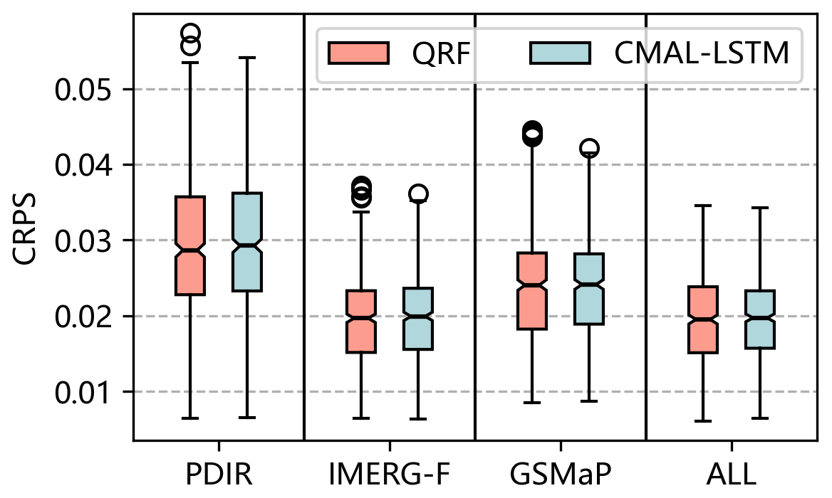
Overall, the QRF and CMAL-LSTM models demonstrate similar performance in terms of CRPS and twCRPS across all threshold conditions (as shown in Figs. 4 and S5). However, it is noteworthy that the QRF model exhibits more outliers compared with the CMAL-LSTM model, indicating that the latter is more stable across sub-basins. When it comes to different precipitation-driven streamflow inputs, the IMERG-F-QRF and IMERG-F-CMAL-LSTM experiments have median CRPS values of 0.0197 and 0.0199, respectively, for 522 sub-basins; the GSMaP-QRF and GSMaP-CMAL-LSTM experiments have median CRPS values of 0.024 and 0.0241, respectively; and the PDIR-QRF and PDIR-CMAL-LSTM experiments have median CRPS values of 0.0287 and 0.0292, respectively. The results show that IMERG-F performs better than GSMaP, and both bias-corrected products outperform the near-real-time product PDIR in post-processing performance. The results of the multi-product approach (All) are close to those of IMERG-F but better than those of PDIR and GSMaP. As the threshold conditions increase, the performance of the multi-product approach is slightly worse than that of IMERG-F (Fig. S5). This suggests that introducing features that perform well in a model, such as IMERG-F-driven raw streamflow, can improve the performance of post-processing models, but introducing features that perform poorly, such as GSMaP- and PDIR-driven raw streamflow, can worsen the performance of post-processing model. The results indicate that the QRF and CMAL-LSTM models can automatically perform feature filtration but cannot completely avoid learning from disruptive information. Using IMERG-F-driven raw streamflow as input, the post-processing models perform better than when driven by the other two products as input features, which is related to the quality of IMERG-F features. In terms of temporal correlation and bias, IMERG-F is the optimal product. The raw streamflow simulation of GSMaP performs worse than PDIR, but the post-processing model performs better than PDIR. The reason is that comparing to PDIR, raw streamflow of GSMaP has higher temporal correlation and better autocorrelation skill as input features. This leads to PDIR being the worst-performing post-processing experiment among the selected datasets.
In addition to their overall performance (Fig. 4), the QRF and CMAL-LSTM models exhibit similar spatial performance, as is reported in Fig. 5. Compared to PDIR and GSMaP, IMERG-F and multi-product results achieve relatively good performance in most of the 522 sub-basins. PDIR performs the worst, which inherently is attributed to its poorer input features, such as low autocorrelation skill of streamflow. The third row in the Fig. 5 (i.e. Fig. 5i–l) shows that the differences between QRF and CMAL-LSTM are mostly within 10 %. However, the introduction of multi-product features increased the gap between them, indicating that CMAL-LSTM has an advantage over the QRF model in processing multi-dimensional features. In the PDIR experiment, the QRF model demonstrates superior performance in 68.2 % of the sub-basins (356 out of 522), while the CMAL-LSTM model performs better in the remaining 31.8 % of sub-basins. Regarding the experiments conducted on IMERG-F, GSMaP, and multi-product (All) simulations, the proportions of QRF and CMAL-LSTM models are 65.5 % and 34.5 %, 54.2 % and 45.8 %, and 64.6 % and 35.4 %, respectively.
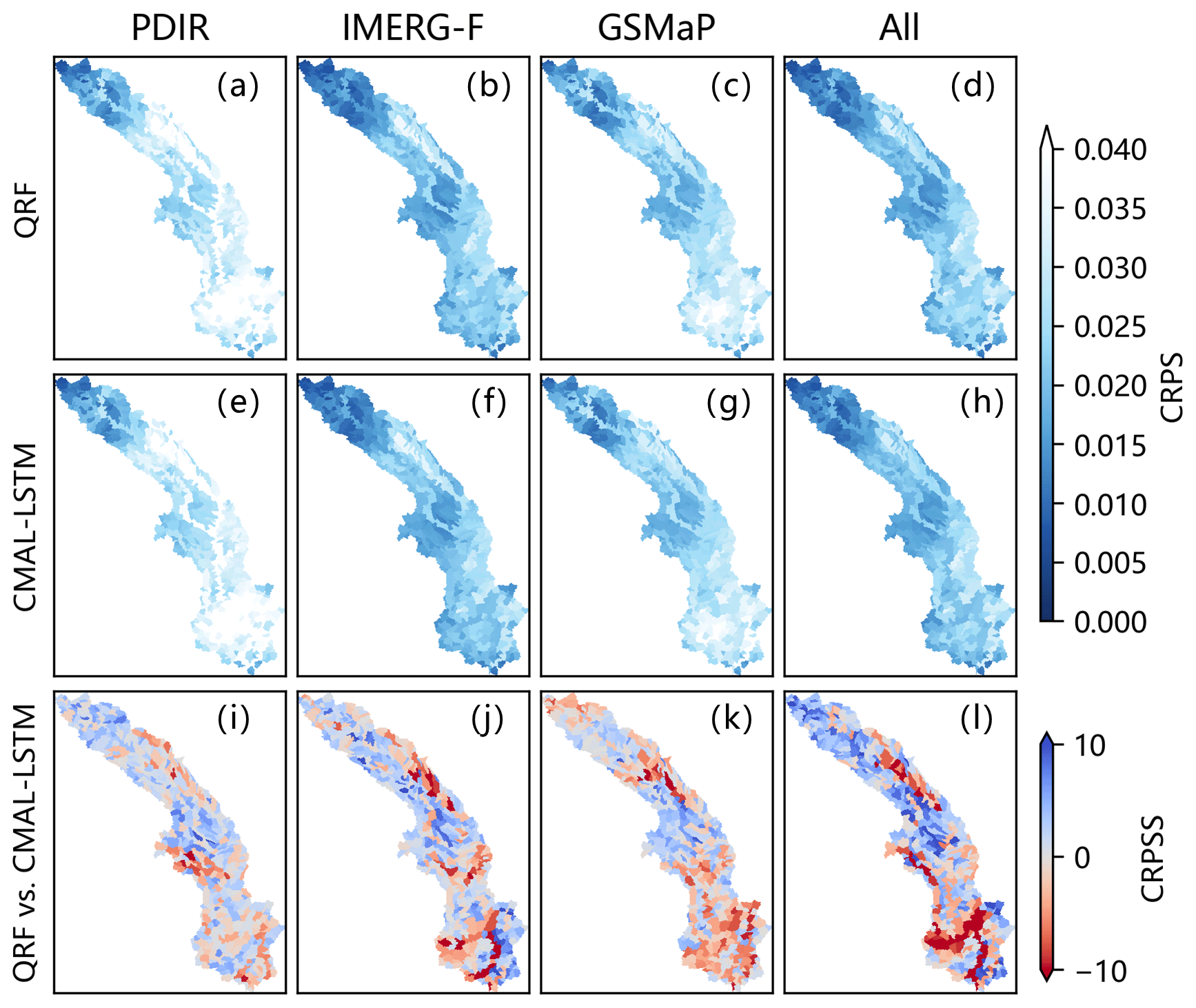
Figure 5The spatial distribution of CRPS and CRPSS for different post-processing experiments.
4.2.2 The relationship between model performance and flow accumulation area (FAA)
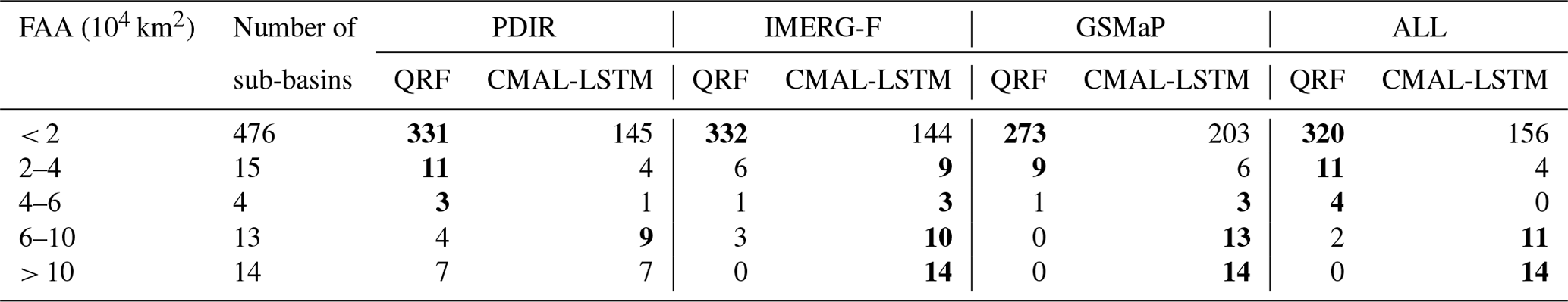
To further investigate the differences between the two post-processing models, the relationship between the CRPS/CRPSS metrics and FAA of sub-basins is presented in Fig. 6. Overall, the CRPS values of both post-processing models increase with increasing FAA, which is related to the streamflow amplitude of different sub-basins. Therefore, the relationship between the CRPSS score and FAA as reported in Fig. 6e–h is of interest to compare the differences between the two post-processing models. It is observed that when FAA is small, the QRF model performance is superior to the CMAL-LSTM model. However, as FAA increases, the post-processing skill of the CMAL-LSTM model surpasses that of the QRF model. Additionally, the sub-basins are categorized, based on their size, into five intervals: less than 20 000, 20 000–40 000, 40 000–60 000, 60 000–100 000 km2, and greater than 100 000 km2. The corresponding number of sub-basins for each of the five intervals is 476, 15, 4, 13, and 14, respectively. The statistics of model performance in different FAA intervals are summarized in Table 2. In sub-basins with FAA less than 20 000 km2, the QRF model shows a better performance. In the PDIR experiment, the QRF model has a higher CRPS value in 69.5 % of sub-basins. In the IMERG-F, GSMaP, and multi-product experiments, the percentage of sub-basins where the QRF model outperforms the CMAL-LSTM model is 69.7 %, 57.4 %, and 67.2 %, respectively. In sub-basins with FAA greater than 60 000 km2, the CMAL-LSTM model shows an absolute advantage. In the PDIR experiment, the CMAL-LSTM model has a higher CRPS value in 16 sub-basins. In the IMERG-F, GSMaP, and multi-product experiments, the number of sub-basins where the CMAL-LSTM model has a higher CRPS value is 24, 27, and 25, respectively.
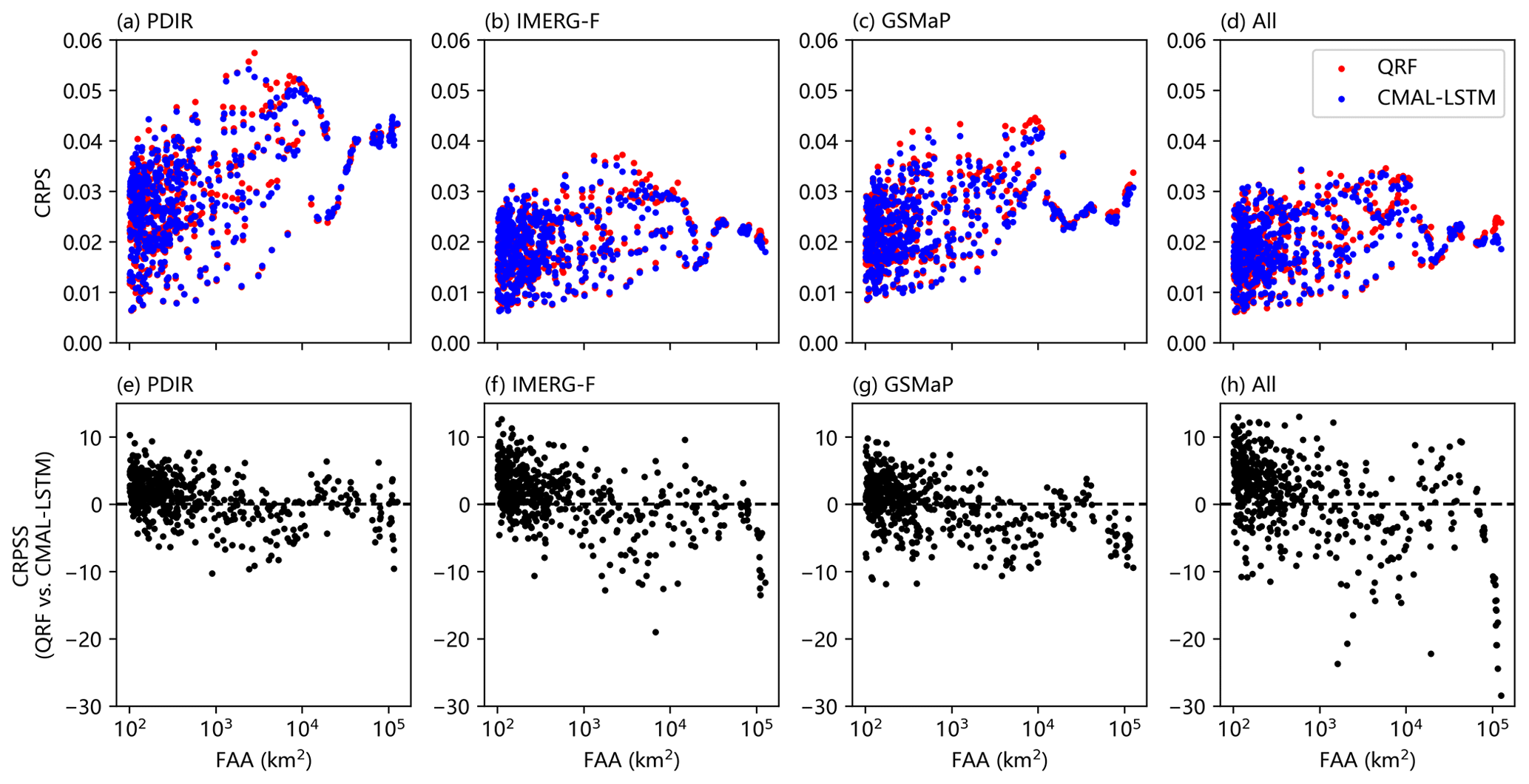
Table 2The probabilistic performance of two post-processing models for different FAA intervals. The bold numbers indicate better performance in each group.
4.2.3 Reliability and sharpness
The reliability diagram is further used to diagnose the difference in post-processing model performance in terms of reliability. To distinguish the differences in model performance of the CMAL-LSTM and QRF models with the change of FAA, the calculation of the reliability diagram is divided into two parts. One part of the analysis focuses on sub-basins with a FAA less than 60 000 km2, as illustrated in Fig. 7a–c. This analysis combines all the streamflow predictions obtained from the 495 sub-basins within this size range. The second part of the analysis focuses on sub-basins with a FAA greater than 60 000 km2, as depicted in Fig. 7d–f. This analysis involves combining all the streamflow predictions from the 27 sub-basins within this size range. Overall, when FAA is less than 60 000 km2, the performance of the two post-processing models is similar. The QRF model is slightly better than the CMAL-LSTM model. Except for the PDIR experiments, all experiments have a high reliability. As the threshold increases, all experiments show an increasing deviation from the diagonal line and a decrease in reliability. Moreover, when FAA of sub-basin exceeds 60 000 km2, the reliability of the post-processing experiments declines, and the CMAL-LSTM model performs slightly better than the QRF model, with more points distributed along the diagonal line. As the threshold increases, the curve becomes more oscillatory, resulting in a significant decrease in reliability. Especially under extreme conditions and as is shown in Fig. 7f, the difference between the two post-processing models is large, with the CMAL-LSTM performing relatively better.
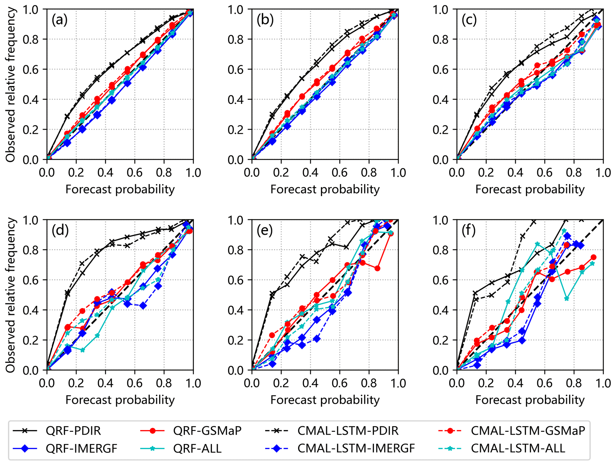
Figure 7Reliability diagrams: (a) 80 %, (b) 90 %, and (c) 95 % percentiles of observations for the sub-basins with FAA less than 60 000 km2 and (d) 80 %, (e) 90 % and (f) 95 % percentiles of observations for the sub-basins with FAA greater than 60 000 km2.
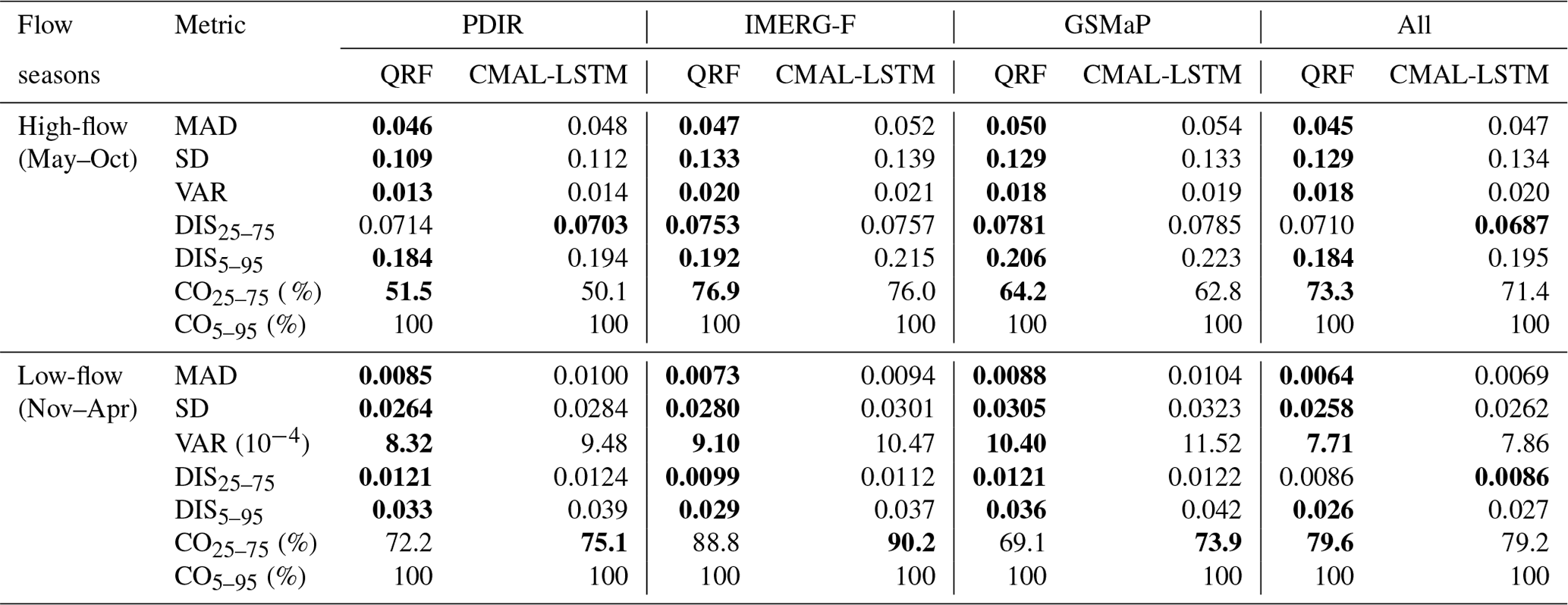
Sharpness describes the variability properties of predictive distribution and can be used to assess the differences between post-processing models from the uncertainty estimation perspective. To eliminate the influence of different flow regimes, all data are divided into high-flow (May to October) and low-flow seasons (November to April). Sharpness metrics are calculated separately for each sub-basin. The average values of the metrics for all 522 sub-basins are listed in Table 3. The results show that, on average across all 522 sub-basins, the QRF model produces narrower prediction intervals than the CMAL-LSTM model during both high and low-flow seasons, indicating higher sharpness of the QRF model compared to CMAL-LSTM. This partially explains why the QRF model has higher CRPS values in most sub-basins. It is worth noting that the QRF model shows high coverage of the observations as well as narrower prediction intervals specifically during high-flow seasons. The average coverage of observations for the 25th to 75th quantiles (CO25–75) is 1.5 % higher for the QRF than for the CMAL-LSTM model. However, a wider prediction interval of the CMAL-LSTM model results in higher coverage of observations during low-flow seasons. The average coverage of observations for the 25th to 75th quantiles (CO25–75) is 2 % higher for the CMAL-LSTM than for the QRF model. Interestingly, the 90 % prediction intervals obtained by both post-processing methods contain 100 % of the observations, based on the average values across all 522 sub-basins during both high- and low-flow seasons.
Table 3Sharpness statistics in high-flow and low-flow seasons. The bold numbers indicate better performance in each group.
4.3 Deterministic (single-point) assessment
Although the post-processing model proposed in this study is probabilistic, decision-makers tend to prefer deterministic (single-point) prediction. Therefore, the average of the probability members is utilized as deterministic predictions to further compare the prediction accuracy of the models. Also, it can be viewed as a post hoc model examination.
4.3.1 Overall model performance
Figure 8 shows the performance evaluation of the streamflow simulations before (RAW) and after post-processing using the QRF and CMAL-LSTM models for 522 sub-basins. PCC, RB, and NSE are used as performance metrics, with each sub-basin being evaluated separately. The median and mean of each metric across all 522 sub-basins are computed and reported in the first three columns of Table 4. The results indicate that both post-processing models significantly improved the simulation performance over the uncorrected streamflow. However, the CMAL-LSTM model consistently outperforms the QRF model across the precipitation products and the sub-basins.
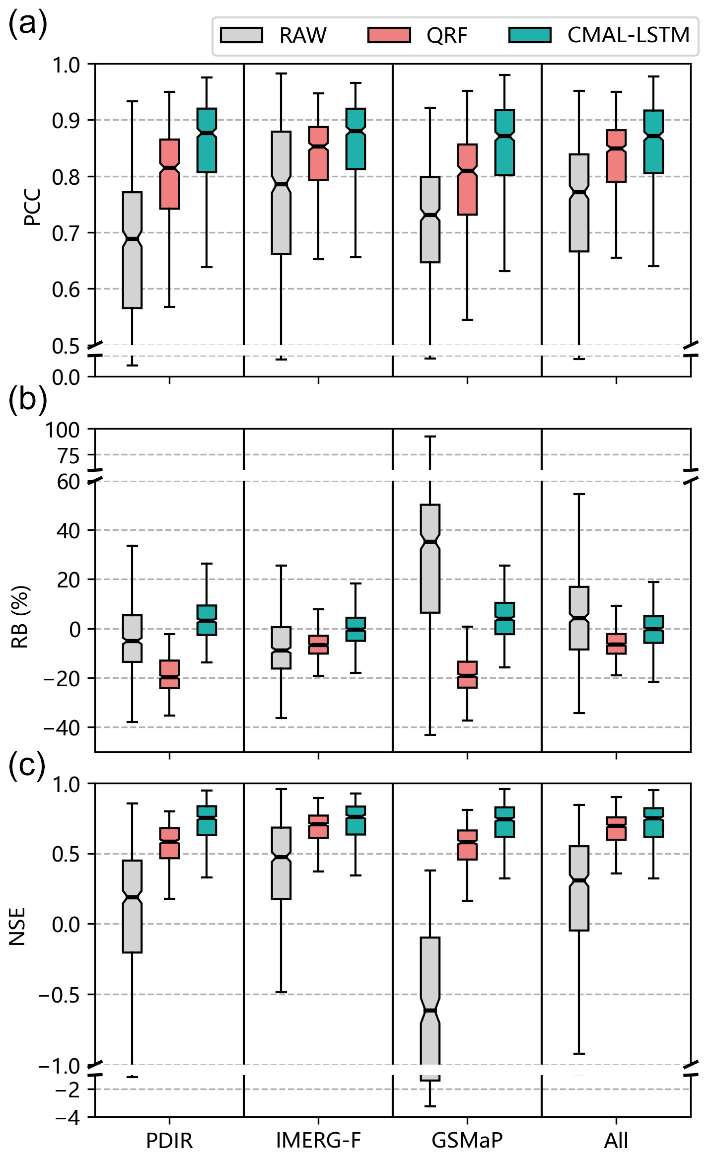
Figure 8Box plots of different model performance in 522 sub-basins. (a) PCC, (b) RB, and (c) NSE.
Figure 9 illustrates the spatial characteristics of the NSE improvement in streamflow simulations obtained through model comparison. Compared to the raw simulations (RAW), both QRF and CMAL-LSTM models exhibit significant improvements in almost all sub-basins. Among all post-processing experiments, GSMaP-CMAL-LSTM and GSMaP-QRF provide the most significant improvement in accuracy due to the poorer performance of the raw GSMaP-driven streamflow simulations. Conversely, the absolute NSE improvement brought by post-processing models is relatively small for the IMERG-F-driven streamflow simulations, and even a slight performance decline in 14.8 % of sub-basins is observed in the IMERG-F-QRF experiment (Fig. 9b). Compared to CMAL-LSTM, the QRF model does not show its advantage of deterministic (single-point) estimation in almost all sub-basins. The maximum difference in model performance appears in GSMaP experiments, followed by PDIR, IMERG-F, and multi-product (All) experiments. This indicates that the deterministic (single-point) estimation ability of the QRF model differs significantly from the CMAL-LSTM model for streamflow with poor raw simulation.
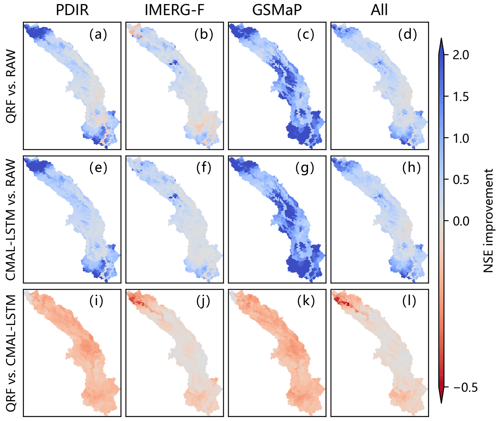
Figure 9The spatial distribution of NSE improvement (NSEPP−NSEraw) between (a–d) QRF and RAW, (e–h) CMAL-LSTM and RAW, and (i–l) QRF and CMAL-LSTM in 522 sub-basins.
4.3.2 The relationship between model performance and flow accumulation area (FAA)
Based on the spatial distribution shown in Fig. 9, the relationship between model performance and the flow accumulation area (FAA) of the sub-basin is further investigated, following a similar analysis approach as in Sect. 4.2.2 and Fig. 6. In Fig. 10, we observe a consistent trend: as FAA of the sub-basin increases, the performance of the model also increases. Notably, the CMAL-LSTM model consistently surpasses the QRF model across all experiments, which is further supported by the statistics in Table S2. However, as FAA of sub-basin increases, the performance gap between the CMAL-LSTM model and QRF model begins to diminish, especially in the IMERG-F driven experiment. In contrast, for experiments such as PDIR, GSMaP, and multi-product (All), the increase in FAA has little effect on the performance difference between the CMAL-LSTM and QRF models. This suggests that highly biased information from raw streamflow simulation has a greater impact on the QRF than on the CMAL-LSTM model.
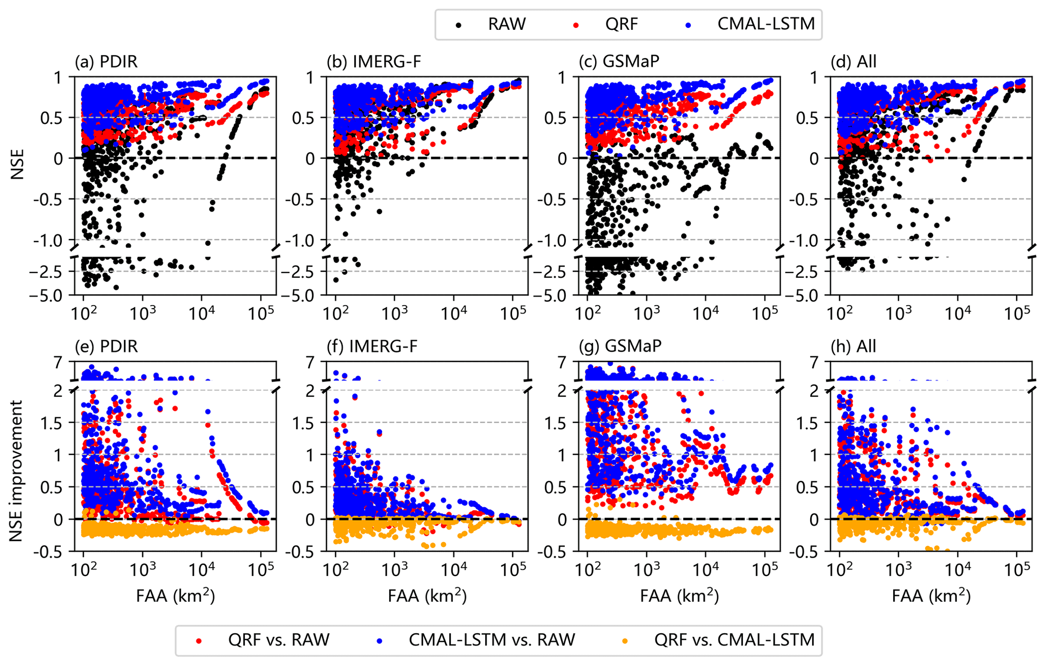
Figure 10The relationships between (a–d) NSE and FAA and between (e–h) NSE improvement (NSEPP−NSEraw) and FAA.
4.3.3 High-flow, low-flow, and peak timing
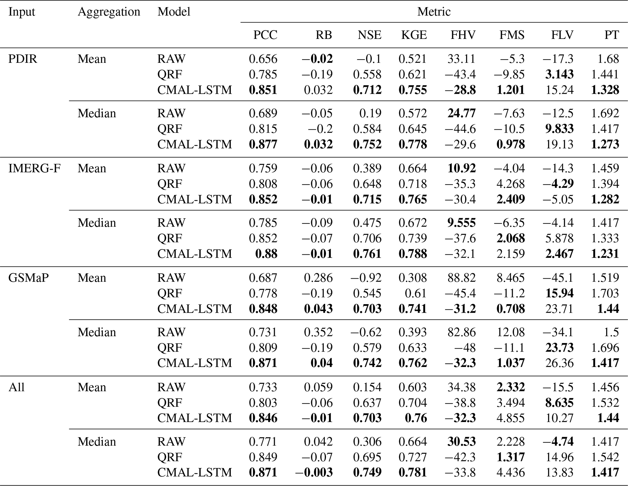
Table 4 summarizes the means and medians of integrated metrics and flow regime indicators for the 522 sub-basins in different experiments. The first three columns of the table are the same as the metrics used in Fig. 8. PCC and RB are the components of the Nash–Sutcliffe efficiency (NSE). In order to guarantee the consensus of the results, another integrated indicator, the KGE, is also calculated. The KGE performs identically to the NSE, confirming the superiority of the CMAL-LSTM model. The last four columns of the table are flow-related indicators. Overall, the CMAL-LSTM model remains the best, except for the low-flow bias (FLV), where the QRF model is more effective. However, as indicated by the high-flow bias (FHV), both post-processing models have limitations in handling flood peaks. Regardless of the precipitation product used to drive the streamflow simulations, the bias of the flood peak changes from an overestimation (RAW) to an underestimation (post-processing). In addition, there is a certain degree of deviation in the simulations of peak time. Flood peaks have always posed a challenging problem in hydrological simulation due to many factors, such as spatial and temporal variability in rainfall extreme, soil moisture conditions, and catchment characteristics (Brunner et al., 2019; Jiang et al., 2022). Furthermore, slight deviations can lead to significant discrepancies in flood risk assessments (Parodi et al., 2020). Given these challenges, the necessity of probabilistic post-processing is highlighted.
Table 4Summary of integrated metrics and flow regime indicators of different models in 522 sub-basins. The bold numbers indicate better performance in each group.
5.1 Model comparison
Previous studies have demonstrated that the quantile regression forests (QRF) approach outperforms other quantile-based models, such as quantile regression and quantile neural networks (Taillardat et al., 2016; Tyralis et al., 2019; Tyralis and Papacharalampous, 2021). Additionally, recent research has indicated the effectiveness of mixture density networks based on the countable mixtures of asymmetric Laplacians models and long short-term memory networks (CMAL-LSTM) for hydrological probabilistic modelling (Klotz et al., 2022). In terms of reliability and sharpness evaluation for probabilistic prediction, CMAL-LSTM has been proven to achieve the best results compared to other models such as LSTM coupled with Gaussian mixture models, uncountable mixtures of asymmetric Laplacians models, and Monte Carlo dropout. These findings suggest that currently, QRF and CMAL-LSTM are the state of the art and the most effective machine learning and deep learning models for hydrological probabilistic modelling. In this study, we conducted a comprehensive evaluation of the performance of these two advanced data-driven models in the context of streamflow probabilistic post-processing.
Our findings suggest that the QRF model outperformed the CMAL-LSTM model in terms of probability prediction in most sub-basins. And the performance difference between the two models was found to be associated with the catchment area of the sub-basins. The QRF model was superior in sub-basins with smaller catchment area, while the CMAL-LSTM model demonstrated better performance in larger sub-basins. However, when evaluated from a deterministic standpoint, the CMAL-LSTM model achieved higher NSE scores than the QRF model across nearly all sub-basins. The authors believe that the primary reason for the inconsistency in model performance is due to the differences in their respective model structure. As illustrated in Fig. 2, the QRF model and the CMAL-LSTM model have dissimilar probabilistic procedure.
First, the QRF model and the CMAL-LSTM model differ in their treatment of input features. Specifically, the QRF model utilizes time embedding to flatten time-series features as input for the model. In contrast, the CMAL-LSTM model is capable of better learning the temporal autocorrelation of input features due to the inherent time-series learning capabilities of LSTM. As a result, the CMAL-LSTM model is more responsive to the autocorrelation of uncorrected streamflow features compared to the QRF model. The results depicted in Fig. S6 provide evidence to support the interpretation that the performance difference between the QRF model and the CMAL-LSTM model is related to the autocorrelation of input features. The CMAL-LSTM model performs better in sub-basin no. 250, where streamflow feature autocorrelations are more skilful, than in sub-basin no. 10, where streamflow feature autocorrelation skills are lacking.
Second, the QRF model and CMAL-LSTM differ in how they generate probabilistic members. The QRF model calculates the final probabilistic members by grouping them based on a predetermined number of quantiles (100 in this study). In contrast, the CMAL-LSTM model first specifies the form of the probabilistic distribution, then learns the parameters of the distribution using neural networks, and finally obtains the final probabilistic members by sampling. The QRF model produces an approximate and implicit probabilistic distribution, while the CMAL-LSTM model produces an accurate and explicit probabilistic distribution. Moreover, the predicted distribution from the CMAL-LSTM model using the mixture density function is more flexible. As a result, the QRF model produces narrower prediction intervals compared to the CMAL-LSTM model, as is reported in Table 3. This is especially true when the sub-basin catchment area is smaller, and the streamflow amplitude is lower. This also explains the reason that the QRF model has higher sharpness in these cases compared to the CMAL-LSTM model. Figure S7 presents the hydrograph and prediction intervals in two randomly selected sub-basins as an example. In sub-basin no. 10, the CMAL-LSTM model achieves a balance between the width of the prediction interval and the observation coverage, which is more important for high-flow predictions and also explains why the CMAL-LSTM model has a higher CRPS value in the sub-basin with larger catchment area. In contrast, although the prediction interval of the QRF model is narrower, it is affected by systematic bias. For example, IMERG-F-QRF underestimates the peak flow in the high-flow season, leading to its smaller CRPS value compared to the CMAL-LSTM model. For sub-basin no. 250 with a smaller catchment area, its rainfall-runoff response is faster, and the fluctuation of streamflow is greater. Localized precipitation events can also cause large pulse flow, which is the main feature of flash floods. Therefore, there are relatively more extreme samples. In this case, the QRF model learns and captures more observations with narrower prediction intervals, resulting in a better CRPS value.
Third, the QRF model and CMAL-LSTM model differ in their inference process. The QRF model utilizes a decision tree model as its base learner, which is a classification algorithm based on historical searches, whereas the CMAL-LSTM model uses a neural network with LSTM layer as its base learner, which is a more powerful fitting model. Due to the differences in model structure, the two models have different abilities to handle extreme events. When extreme event samples are limited, the QRF model tends to underestimate predictions due to its historical search-based approach. On the other hand, the CMAL-LSTM uses the mixture density function for extrapolation. However, both post-processing models still underestimates streamflow extreme events. The QRF model exhibits a higher degree of underestimation in sub-basins with larger catchment areas, resulting in unsatisfactory performance compared to the CMAL-LSTM model in these regions. These discrepancies also lead to lower NSE scores for the QRF model across all sub-basins, as the squared term in the NSE metric increases the sensitivity to high-flow processes, which is reported in Fig. S8.
Furthermore, besides examining the differences in model performance, we investigated the effects of different input features on the post-processing model by using three different satellite precipitation products in this study. We observed a cascading impact on model performance in the rainfall-runoff and post-processing processes. Given a fixed hydrological model, in areas with a small catchment area, the response of streamflow to precipitation is quicker, and the quality of satellite precipitation products directly influences the quality of streamflow prediction through the rainfall-runoff process. The temporal correlation of satellite precipitation determines the temporal correlation of streamflow prediction. Deviations in satellite precipitation led to the biased streamflow prediction and have a more significant effect on the NSE score of streamflow prediction. This explains the reason that IMERG-F is optimal and PDIR is superior to GSMaP. During the transfer process from raw streamflow to post-processed streamflow, the autocorrelation skill of the raw runoff dictates the performance of the streamflow post-processing model. This clarifies why IMERG-F is still optimal, but GSMaP is superior to PDIR. Based on the results of the multi-product experiment, we observed that the post-processing model can learn better features to a larger extent; however, it cannot completely filter out the information that affects the model accuracy. Regarding information filtering, the CMAL-LSTM model surpasses the QRF model. These findings suggest that although streamflow post-processing can enhance model performance, opting for the best-quality product is still a prudent decision when multiple precipitation products are available, and it can also save more computing resources. Another strategy is to execute precipitation post-processing before the hydrological model, which can assist the model in better learning the features and ultimately improving model performance.
5.2 Limitations and future work
This study provides a systematic evaluation of QRF and CMAL-LSTM models in probabilistic streamflow post-processing, yielding valuable insights and practical experience on model selection. However, there are still some deficiencies that need to be addressed in future research. The avenues for further investigations are summarized as follows.
First, we used simulated streamflow driven by observed precipitation as a proxy for true streamflow. This study diverges from previous research by focusing on sub-basin scale streamflow post-processing in a nested basin comprised of 522 sub-basins exhibiting varying flow accumulation areas, ranging from 100 to 127 164 km2. To achieve the streamflow post-processing for these 522 sub-basins, corresponding streamflow observations are required, but such data are not readily available. As an alternative, we employed streamflow simulations generated by a calibrated hydrological model driven by observed precipitation. This approach yields a post-processing model performance that closely approximates the given reference; however, it is not an exact representation of actual streamflow post-processing. Despite this limitation, the reference generated was used to evaluate the performance of various post-processing models. Future studies could conduct a more in-depth comparison of different post-processing models in basins with more streamflow records. Nonetheless, our dataset remains scarce in the current community, and we have made it available along with this study to enable other researchers to evaluate and compare different methods against the benchmark presented in this study (Zhang et al., 2022b).
Second, there exists data imbalance among the studied sub-basins. Among the selected 522 sub-basins, it can be observed that model performance is related to the catchment size. However, the number of sub-basins corresponding to each of the five intervals (100–20 000, 20 000–40 000, 40 000–60 000, 60 000–100 000 km2, and greater than 100 000 km2) is 476, 15, 4, 13, and 14, respectively. Only 5.2 % of the sub-basins have a catchment area larger than 60 000 km2. This could potentially affect the generality of conclusions drawn. To address this limitation, more extensive and balanced datasets (such as Caravan, Kratzert et al., 2023) are needed to be utilized to achieve further validation of the research findings and a better understanding of different post-processing models.
Third, the selection of input features and hydrological models could be extended. In order to maintain model complexity and keep computational costs low, this study only used one variable, uncorrected streamflow, as the predictor. However, there are more variables that can be used as predictors, including other meteorological variables such as temperature and wind speed (Frame et al., 2021). In addition, basin-related attributes can provide us with local information, which is particularly helpful for the prediction in ungauged areas. In previous studies, all of these variables have been shown to have varying degrees of contributions to the model (Jiang et al., 2022). For post-processing, there are also studies that use model state variables and other output variables as predictors (Frame et al., 2021), which can provide us with information about the hydrological processes and increase the physical interpretability of the post-processing framework (Razavi, 2021; Tsai et al., 2021). However, state variables and outputs generated by hydrological models tend to be biased due to inherent bias in the satellite precipitation. It is unclear whether this is helpful for streamflow post-processing and requires further exploration. In terms of hydrological model selection, only the distributed time-variant gain model (DTVGM) was used to simulate streamflow from three different satellite precipitation products to increase the diversity of post-processing experiments. By doing so, the other two sources of uncertainty, namely, model structure and parameters, were eliminated, since the focus of this study was on comparing post-processing model with input uncertainty. It is worth noting that in addition to input uncertainty, hydrological model structure and parameter uncertainty are also significant sources of uncertainty, as highlighted by Herrera et al. (2022) and Mai et al. (2022a, b). For future post-processing model comparisons, we suggest adopting the approach of using multiple hydrological models to analyse the uncertainty of model structure and parameters (Ghiggi et al., 2021; Troin et al., 2021; Mai et al., 2022a, b).
Fourth, the post-processing models have limitations in handling streamflow extreme events, as observed through comparative analysis and visualization as reported in Table 4 and Fig. S8. The QRF model is based on a historical analogy search, wherein the model finds a group of similar samples and averages them at the leaf nodes to obtain the final prediction (Li and Martin, 2017). As a result, the limited number of samples, particularly for extreme events, hinders its ability to predict such events. However, this limitation can be addressed by introducing additional parameter mixing methods, such as combining QRF and extreme value distribution. Previous attempts, such as combining QRF and extended generalized Pareto distribution, have shown promising results (Taillardat et al., 2019). Nonetheless, these mixing methods add complexity to the model and require additional calibration of hyperparameters. The CMAL-LSTM model is also constrained by the number of extreme event samples, but its performance in these extreme events exceeds that of the QRF model. Additionally, the CMAL-LSTM model chosen in this study is a mixture density network and the corresponding parameters are directly learned through neural network optimization algorithms like gradient descent. The authors believe that collecting more data samples and introducing additional predictors and distribution functions for extreme events can lead to further improvements.
Finally, it is important to constantly enhance and update the model comparison iteratively. The CMAL-LSTM model was selected based on its superior performance as proposed by Klotz et al. (2022). They also evaluated two other hybrid density networks and a probabilistic method using Monte Carlo dropout. Additionally, there are other probabilistic prediction methods such as the variational inference (Li et al., 2021) and generative adversarial networks (Pan et al., 2021). In a rapidly evolving community, new methods can be applied and tested to further improve the performance of streamflow post-processing in future research.
In this study, a series of well-designed experiments to compare the performance of two state-of-the-art models for streamflow probabilistic post-processing were conducted: a machine learning model (quantile regression forests) and a deep learning model (countable mixtures of asymmetric Laplacians long short-term memory network). Using observed precipitation and three different satellite precipitation products to drive the calibrated hydrological model, we generated a large-sample dataset of 522 sub-basins with paired streamflow reference and biased streamflow simulations. We evaluated the model performance from both probabilistic and deterministic perspectives, including reliability, sharpness, accuracy, and flow regime, through intuitive case studies. These experiments established a path for understanding the model differences in probabilistic modelling and post-processing, provided practical experience for model selection, and extracted insights for model improvement. It also serves as a reference for establishing benchmark tests for model evaluation, including dataset construction and metrics selection. Furthermore, streamflow post-processing provides dependable data support for a range of downstream tasks, such as flood risk analysis, reservoir scheduling, and water resource management. The empirical findings of this study for the two post-processing models are summarized below.
-
Based on the probabilistic assessment, the QRF and CMAL-LSTM models exhibit comparable performance. However, their model differences are correlated with the flow accumulation area (FAA) of sub-basins. In cases where the catchment area of a sub-basin is small, the QRF model generates a narrower prediction interval, resulting in better CRPS scores compared to the CMAL-LSTM model in most sub-basins. Conversely, in larger sub-basins (over 60 000 km2 in this study), the CMAL-LSTM model outperforms the QRF model due to its ability to learn autocorrelation skills of features and capture more extreme values.
-
Based on the deterministic assessment, it can be concluded that the CMAL-LSTM model performs better than the QRF model in capturing high-flow process and flow duration curve. On the other hand, the QRF model tends to underestimate the high-flow process, resulting in worse NSE score across all sub-basins. Both models, however, have the issue of underestimating flood peaks due to sparse samples of extreme events.
-
The impact of the inherent uncertainties from different satellite precipitation products on streamflow simulations is reduced by both models. However, the performance of the post-processing models does not improve further in the multi-product experiments. Instead, the inclusion of heavily biased inputs leads to a deterioration in model performance. Recommending the choice of a single precipitation product that is best suited to the task at hand is expected to safeguard the model performance and reduce the computational cost.
-
Given the performance of post-processing models, the authors believe that these models have the potential to be applied to other sources of uncertainty that affect hydrological modelling, such as model structure and parameter uncertainty.
The GPM IMERG Final Run is freely available at GES DISC (https://doi.org/10.5067/GPM/IMERGDF/DAY/06, Huffman et al., 2019) The PDIR data can be freely downloaded from CHRS Data Portal (http://chrsdata.eng.uci.edu/, Nguyen et al., 2019). The GSMaP data are publicly available (at https://sharaku.eorc.jaxa.jp/GSMaP/index.htm, Kubota et al., 2023). The CMA precipitation observations are provided by the National Meteorological Information Centre of China Meteorological Administration. The soil types are freely available (at http://www.fao.org/soils-portal/soil-survey/soil-maps-and-databases/harmonized-world-soil-database-v12/en/, Fischer et al., 2008). The land use data are freely available from the Chinese National Tibetan Plateau Third Pole Environment Data Centre (at http://data.tpdc.ac.cn/en/data/a75843b4-6591-4a69-a5e4-6f94099ddc2d, CAS-RESDC, 2019). The DEM data are freely available at http://www.gscloud.cn (CAS-CNIC, 2023). The QRF model code is available on GitHub (https://github.com/jnelson18/pyquantrf, last access: 18 December 2023; https://doi.org/10.5281/zenodo.5815105, Jnelson18, 2022). The CMAL-LSTM model code is available on GitHub (https://github.com/neuralhydrology/neuralhydrology, last access: 20 December 2023; Kratzert et al., 2022b). The dataset and results of this study are available on Zenodo (https://doi.org/10.5281/zenodo.7187505) (Zhang et al., 2022b).
The supplement related to this article is available online at: https://doi.org/10.5194/hess-27-4529-2023-supplement.
Conceptualization, YZ, AY, BA, PN, SS, KH, and YW; methodology, YZ and AY; software, YZ and AY; validation, YZ; data curation, YZ, AY, BA, and PN; visualization, YZ; supervision, AY, KH, and SS; project administration, AY and SS; funding acquisition, AY and SS. original draft preparation, YZ; review and editing, YZ, AY, BA, PN, SS, KH, and YW. All authors have read and agreed to the published version of the manuscript.
The contact author has declared that none of the authors has any competing interests.
Publisher’s note: Copernicus Publications remains neutral with regard to jurisdictional claims made in the text, published maps, institutional affiliations, or any other geographical representation in this paper. While Copernicus Publications makes every effort to include appropriate place names, the final responsibility lies with the authors.
This research is jointly supported by the Natural Science Foundation of China (nos. 42171022, 51879009), the Second Tibetan Plateau Scientific Expedition and Research Program (no. 2019QZKK0405), the National Key Research and Development Program of China (no. 2018YFE0196000), and the U.S. Department of Energy (DOE Prime Award DE-IA0000018). The authors wish to acknowledge Nunzio Romano for his editorial contributions and extend their gratitude to the three anonymous referees for their valuable reviews of this paper.
This research has been supported by the Natural Science Foundation of China (grant nos. 42171022 and 51879009), the Second Tibetan Plateau Scientific Expedition and Research Program (grant no. 2019QZKK0405), the National Key Research and Development Program of China (grant no. 2018YFE0196000), and the U.S. Department of Energy (DOE Prime Award DE‐IA0000018).
This paper was edited by Nunzio Romano and reviewed by three anonymous referees.
Althoff, D., Rodrigues, L. N., and Bazame, H. C.: Uncertainty quantification for hydrological models based on neural networks: the dropout ensemble, Stoch. Env. Res. Risk A., 35, 1051-1067, https://doi.org/10.1007/s00477-021-01980-8, 2021.
Bellier, J., Zin, I., and Bontron, G.: Generating coherent ensemble forecasts after hydrological postprocessing: Adaptations of ECC-based methods, Water Resour. Res., 54, 5741–5762, https://doi.org/10.1029/2018WR022601, 2018.
Beven, K.: Changing ideas in hydrology – the case of physically-based models, J. Hydrol., 105, 157–172, https://doi.org/10.1016/0022-1694(90)90161-P, 1989.
Bogner, K. and Pappenberger, F.: Multiscale error analysis, correction, and predictive uncertainty estimation in a flood forecasting system, Water Resour. Res., 47, e2010WR009137, https://doi.org/10.1029/2010WR009137, 2011.
Bormann, K. J., Evans, J. P., and McCabe, M. F.: Constraining snowmelt in a temperature-index model using simulated snow densities, J. Hydrol., 517, 652–667, https://doi.org/10.1016/j.jhydrol.2014.05.073, 2014.
Bröcker, J.: Evaluating raw ensembles with the continuous ranked probability score, Q. J. Roy. Meteor. Soc., 138, 1611–1617, https://doi.org/10.1002/qj.1891, 2012.
Brunner, M. I., Hingray, B., Zappa, M., and Favre, A. C.: Future trends in the interdependence between flood peaks and volumes: Hydro-climatological drivers and uncertainty, Water Resour. Res., 55, 4745–4759, https://doi.org/10.1029/2019WR024701, 2019.
Chawanda, C. J., George, C., Thiery, W., Griensven, A. V., Tech, J., Arnold, J., and Srinivasan, R.: User-friendly workflows for catchment modelling: Towards reproducible SWAT+ model studies, Environ. Modell. Softw., 134, 104812, https://doi.org/10.1016/j.envsoft.2020.104812, 2020.
Chen, H., Yong, B., Shen, Y., Liu, J., Hong, Y., and Zhang, J.: Comparison analysis of six purely satellite-derived global precipitation estimates, J. Hydrol., 581, 124376, https://doi.org/10.1016/j.jhydrol.2019.124376, 2020.
Chinese Academy of Sciences Computer Network Information Center (CAS-CNIC): The National Aeronautics and Space Administration Shuttle Radar Topographic Mission (NASA SRTM): Digital elevation model data republication, GSCLOUD [data set], http://www.gscloud.cn, last access: 18 December 2023.
Chinese Academy of Sciences Resource and Environmental Science Data Center (CAS-RESDC): Landuse dataset in China (1980–2015), National Tibetan Plateau/Third Pole Environment Data Center [data set], http://data.tpdc.ac.cn/en/data/a75843b4-6591-4a69-a5e4-6f94099ddc2d (last access: 18 December 2023), 2019.
Clark, M. P., Nijssen, B., Lundquist, J. D., Kavetski, D., Rupp, D. E., Woods, R. A., Freer, J. E., Gutmann, E. D., Wood, A. W., Brekke, L. D., Arnold, J. R., Gochis, D. J., and Rasmussen, R. M.: A unified approach for process-based hydrologic modelling: 1. Modelling concept, Water Resour. Res., 51, 2498–2514, https://doi.org/10.1002/2015WR017198, 2015.
Corzo Perez, G. A., van Huijgevoort, M. H. J., Voß, F., and van Lanen, H. A. J.: On the spatio-temporal analysis of hydrological droughts from global hydrological models, Hydrol. Earth Syst. Sci., 15, 2963–2978, https://doi.org/10.5194/hess-15-2963-2011, 2011.
Cunha, L. K., Mandapaka, P. V., Krajewski, W. F., Mantilla, R., and Bradley, A. A.: Impact of radar-rainfall error structure on estimated flood magnitude across scales: An investigation based on a parsimonious distributed hydrological model, Water Resour. Res., 48, W10515, https://doi.org/10.1029/2012WR012138, 2012.
Dembélé, M., Hrachowitz, M., Savenije, H. H. G., Mariéthoz, G., and Schaefli, B.: Improving the Predictive Skill of a Distributed Hydrological Model by Calibration on Spatial Patterns With Multiple Satellite Data Sets, Water Resour. Res., 56, e2019WR026085, https://doi.org/10.1029/2019WR026085, 2020.
Dong, J., Crow, W. T., and Reichle, R.: Improving Rain/No-Rain Detection Skill by Merging Precipitation Estimates from Different Sources, J. Hydrometeorol., 21, 2419–2429, https://doi.org/10.1175/JHM-D-20-0097.1, 2020.
Du, C., Ye, A., Gan, Y., You, J., Duan, Q., Ma, F., and Hou, J.: Drainage network extraction from a high-resolution DEM using parallel programming in the .NET Framework, J. Hydrol., 555, 506–517, https://doi.org/10.1016/j.jhydrol.2017.10.034, 2017.
Evin, G., Lafaysse, M., Taillardat, M., and Zamo, M.: Calibrated ensemble forecasts of the height of new snow using quantile regression forests and ensemble model output statistics, Nonlin. Processes Geophys., 28, 467–480, https://doi.org/10.5194/npg-28-467-2021, 2021.
Falck, A. S., Maggioni, V., Tomasella, J., Vila, D. A., and Diniz, F. L. R.: Propagation of satellite precipitation uncertainties through a distributed hydrologic model: A case study in the Tocantins–Araguaia basin in Brazil, J. Hydrol., 527, 943–957, https://doi.org/10.1016/j.jhydrol.2015.05.042, 2015.
Fang, K., Kifer, D., Lawson, K., Feng, D., and Shen, C.: The data synergy effects of time-series deep learning models in hydrology, Water Resour. Res., 58, e2021WR029583, https://doi.org/10.1029/2021WR029583, 2022.
Fischer, G., Nachtergaele, F., Prieler, S., van Velthuizen, H. T., Verelst, L., and Wiberg, D.: Global Agroecological Zones Assessment for Agriculture (GAEZ 2008), IIASA, Laxenburg, Austria and FAO, Rome, Italy, [data set], http://www.fao.org/soils-portal/soil-survey/soil-maps-and-databases/harmonized-world-soil-database-v12/en/ (last access: 18 December 2023), 2008.
Frame, J. M., Kratzert, F., Raney, A., Rahman, M., Salas, F. R., and Nearing, G. S.: Post-Processing the National Water Model with Long Short-Term Memory Networks for Streamflow Predictions and Model Diagnostics, J. Am. Water Resour. As., 57, 885–905, https://doi.org/10.1111/1752-1688.12964, 2021.
Ghiggi, G., Humphrey, V., Seneviratne, S. I., and Gudmundsson, L.: G-RUN ENSEMBLE: A Multi-Forcing Observation-Based Global Runoff Reanalysis, Water Resour. Res., 57, e2020WR028787, https://doi.org/10.1029/2020WR028787, 2021.
Gneiting, T. and Ranjan, R.: Comparing density forecasts using threshold-and quantile-weighted scoring rules, J. Bus. Econ. Stat., 29, 411–422, https://doi.org/10.1198/jbes.2010.08110, 2011.
Gneiting, T., Balabdaoui, F., and Raftery, A. E.: Probabilistic forecasts, calibration and sharpness, J. Roy. Stat. Soc. B, 69, 243–268, https://doi.org/10.1111/j.1467-9868.2007.00587.x, 2007.
Gupta, H. V., Kling, H., Yilmaz, K. K., and Martinez, G. F.: Decomposition of the mean squared error and NSE performance criteria: Implications for improving hydrological modelling, J. Hydrol., 377, 80–91, https://doi.org/10.1016/j.jhydrol.2009.08.003, 2009.
Gou, J., Miao, C., Duan, Q., Tang, Q., Di, Z., Liao, W., Wu, J., and Zhou, R.: Sensitivity Analysis-Based Automatic Parameter Calibration of the VIC Model for Streamflow Simulations Over China, Water Resour. Res., 56, e2019WR025968, https://doi.org/10.1029/2019WR025968, 2020.
Gou, J., Miao, C., Samaniego, L., Xiao, M., Wu, J., and Guo, X.: CNRD v1.0: A High-Quality Natural Runoff Dataset for Hydrological and Climate Studies in China, B. Am. Meteorol. Soc., 102, E929–E947, https://doi.org/10.1175/BAMS-D-20-0094.1, 2021.
Herrera, P. A., Marazuela, M. A., and Hofmann, T.: Parameter estimation and uncertainty analysis in hydrological modelling, Wiley Interdisciplinary Reviews-Water, 9, e1569, https://doi.org/10.1002/wat2.1569, 2022.
Honti, M., Scheidegger, A., and Stamm, C.: The importance of hydrological uncertainty assessment methods in climate change impact studies, Hydrol. Earth Syst. Sci., 18, 3301–3317, https://doi.org/10.5194/hess-18-3301-2014, 2014.
Hou, A. Y., Kakar, R. K., Neeck, S., AA, A., Kummerow, C. D., Kojima, M., Oki, R., Nakamura, K., and Iguchi, T.: The Global Precipitation Measurement Mission, B. Am. Meteorol. Soc., 95, 701–722, https://doi.org/10.1175/BAMS-D-13-00164.1, 2013.
Huffman, G. J., Stocker, E. F., Bolvin, D. T., Nelkin, E. J., and Tan, J.: GPM IMERG Final Precipitation L3 1 day 0.1 degree x 0.1 degree V06, Goddard Earth Sciences Data and Information Services Center (GES DISC), Greenbelt, MD [data set], https://doi.org/10.5067/GPM/IMERGDF/DAY/06, 2019.
Huffman, G. J., Bolvin, D. T., Nelkin, E. J., and Tan, J.: Integrated Multi-satellitE Retrievals for GPM (IMERG) technical documentation, https://gpm.nasa.gov/resources/documents/IMERG-V06-Technical-Documentation (last access: 18 December 2023), 2020.
Jajarmizadeh, M., Harun, S., and Salarpour, M.: A review on theoretical consideration and types of models in hydrology, Journal of Environmental Science and Technology, 5, 249–261, https://doi.org/10.3923/jest.2012.249.261, 2012.
Jiang, L. and Bauer-Gottwein, P.: How do GPM IMERG precipitation estimates perform as hydrological model forcing? Evaluation for 300 catchments across Mainland China, J. Hydrol., 572, 486–500, https://doi.org/10.1016/j.jhydrol.2019.03.042, 2019.
Jiang, S., Zheng, Y., Wang, C., and Babovic, V.: Uncovering Flooding Mechanisms Across the Contiguous United States Through Interpretive Deep Learning on Representative Catchments, Water Resour. Res., 58, e2021WR030185, https://doi.org/10.1029/2021WR030185, 2022.
Jnelson18: jnelson18/pyquantrf: DOI release (v0.0.3doi), Zenodo [code], https://doi.org/10.5281/zenodo.5815105, 2022.
Jolliffe, I. T. and Stephenson, D. B.: Forecast verification: a practitioner's guide in atmospheric science, John Wiley & Sons, https://doi.org/10.1002/9781119960003, 2012.
Kasraei, B., Heung, B., Saurette, D. D., Schmidt, M. G., Bulmer, C. E., and Bethel, W.: Quantile regression as a generic approach for estimating uncertainty of digital soil maps produced from machine-learning, Environ. Modell. Softw., 144, 105139, https://doi.org/10.1016/j.envsoft.2021.105139, 2021.
Khakbaz, B., Imam, B., Hsu, K., and Sorooshian, S.: From lumped to distributed via semi-distributed: Calibration strategies for semi-distributed hydrologic models, J. Hydrol., 418, 61–77, https://doi.org/10.1016/j.jhydrol.2009.02.021, 2012.
Kling, H., Fuchs, M., and Paulin, M.: Runoff conditions in the upper Danube basin under an ensemble of climate change scenarios, J. Hydrol., 424, 264–277, https://doi.org/10.1016/j.jhydrol.2012.01.011, 2012.
Klotz, D., Kratzert, F., Gauch, M., Keefe Sampson, A., Brandstetter, J., Klambauer, G., Hochreiter, S., and Nearing, G.: Uncertainty estimation with deep learning for rainfall–runoff modeling, Hydrol. Earth Syst. Sci., 26, 1673–1693, https://doi.org/10.5194/hess-26-1673-2022, 2022.
Kobold, M. and Sušelj, K.: Precipitation forecasts and their uncertainty as input into hydrological models, Hydrol. Earth Syst. Sci., 9, 322–332, https://doi.org/10.5194/hess-9-322-2005, 2005.
Kratzert, F., Klotz, D., Brenner, C., Schulz, K., and Herrnegger, M.: Rainfall–runoff modelling using Long Short-Term Memory (LSTM) networks, Hydrol. Earth Syst. Sci., 22, 6005–6022, https://doi.org/10.5194/hess-22-6005-2018, 2018.
Kratzert, F., Klotz, D., Shalev, G., Klambauer, G., Hochreiter, S., and Nearing, G.: Towards learning universal, regional, and local hydrological behaviors via machine learning applied to large-sample datasets, Hydrol. Earth Syst. Sci., 23, 5089–5110, https://doi.org/10.5194/hess-23-5089-2019, 2019.
Kratzert, F., Klotz, D., Hochreiter, S., and Nearing, G. S.: A note on leveraging synergy in multiple meteorological data sets with deep learning for rainfall–runoff modeling, Hydrol. Earth Syst. Sci., 25, 2685–2703, https://doi.org/10.5194/hess-25-2685-2021, 2021.
Kratzert, F., Gauch, M., Nearing, G., and Klotz, D.: NeuralHydrology – A Python library for Deep Learning research in hydrology, Journal of Open Source Software, 7, 4050, https://doi.org/10.21105/joss.04050, 2022a.
Kratzert, F., Gauch, M., Nearing, G., and Klotz, D.: NeuralHydrology – A Python library for Deep Learning research in hydrology (v.1.2.3), Zenodo [code], https://doi.org/10.5281/zenodo.6326394, 2022b.
Kratzert, F., Nearing, G., Addor, N., Erickson, T., Gauch, M., Gilon, O., Gudmundsson, L., Hassidim, A., Klotz, D., and Nevo, S.: Caravan – A global community dataset for large-sample hydrology, Sci. Data, 10, 61, https://doi.org/10.1038/s41597-023-01975-w, 2023.
Kubota, T., Shige, S., Hashizume, H., Aonashi, K., Takahashi, N., Seto, S., Hirose, M., Takayabu, Y. N., Ushio, T., and Nakagawa, K.: Global precipitation map using satellite-borne microwave radiometers by the GSMaP project: Production and validation, IEEE T. Geosci. Remote, 45, 2259–2275, https://doi.org/10.1109/TGRS.2007.895337, 2007.
Kubota, T., Aonashi, K., Ushio, T., Shige, S., Takayabu, Y. N., Kachi, M., Arai, Y., Tashima, T., Masaki, T., and Kawamoto, N.: Global Satellite Mapping of Precipitation (GSMaP) products in the GPM era, Satellite Precipitation Measurement, 1, 355–373, https://doi.org/10.1007/978-3-030-24568-9_20, 2020.
Kubota, T., Aonashi, K., Ushio, T., Shige, S., Takayabu, Y. N., Kachi, M., Arai, Y., Tashima, T., Masaki, T., and Kawamoto, N.: Global Satellite Mapping of Precipitation (GSMaP) products, JAXA Global Rainfall Watch [data set], https://sharaku.eorc.jaxa.jp/GSMaP/index.htm (last access: 18 December 2023), 2023.
Lees, T., Buechel, M., Anderson, B., Slater, L., Reece, S., Coxon, G., and Dadson, S. J.: Benchmarking data-driven rainfall–runoff models in Great Britain: a comparison of long short-term memory (LSTM)-based models with four lumped conceptual models, Hydrol. Earth Syst. Sci., 25, 5517–5534, https://doi.org/10.5194/hess-25-5517-2021, 2021.
Li, A. H. and Martin, A.: Forest-type regression with general losses and robust forest, Proceedings of the 34th International Conference on Machine Learning, 70, 2091–2100, 2017.
Li, D., Marshall, L., Liang, Z., Sharma, A., and Zhou, Y., Bayesian LSTM With Stochastic Variational Inference for Estimating Model Uncertainty in Process-Based Hydrological Models, Water Resour. Res., 57, e2021WR029772, https://doi.org/10.1029/2021WR029772, 2021.
Li, D., Marshall, L., Liang, Z., and Sharma, A.: Hydrologic multi-model ensemble predictions using variational Bayesian deep learning, J. Hydrol., 604, 127221, https://doi.org/10.1016/j.jhydrol.2021.127221, 2022.
Li, M., Wang, Q. J., Bennett, J. C., and Robertson, D. E.: A strategy to overcome adverse effects of autoregressive updating of streamflow forecasts, Hydrol. Earth Syst. Sci., 19, 1–15, https://doi.org/10.5194/hess-19-1-2015, 2015.
Li, M., Wang, Q. J., Bennett, J. C., and Robertson, D. E.: Error reduction and representation in stages (ERRIS) in hydrological modelling for ensemble streamflow forecasting, Hydrol. Earth Syst. Sci., 20, 3561–3579, https://doi.org/10.5194/hess-20-3561-2016, 2016.
Li, W., Duan, Q., Miao, C., Ye, A., Gong, W., and Di, Z.: A review on statistical postprocessing methods for hydrometeorological ensemble forecasting, Wiley Interdisciplinary Reviews: Water, 4, e1246, https://doi.org/10.1002/wat2.1246, 2017.
Mai, J., Craig, J. R., Tolson, B. A., and Arsenault, R.: The sensitivity of simulated streamflow to individual hydrologic processes across North America, Nat. Commun., 13, 455, https://doi.org/10.1038/s41467-022-28010-7, 2022a.
Mai, J., Shen, H., Tolson, B. A., Gaborit, É., Arsenault, R., Craig, J. R., Fortin, V., Fry, L. M., Gauch, M., Klotz, D., Kratzert, F., O'Brien, N., Princz, D. G., Rasiya Koya, S., Roy, T., Seglenieks, F., Shrestha, N. K., Temgoua, A. G. T., Vionnet, V., and Waddell, J. W.: The Great Lakes Runoff Intercomparison Project Phase 4: the Great Lakes (GRIP-GL), Hydrol. Earth Syst. Sci., 26, 3537–3572, https://doi.org/10.5194/hess-26-3537-2022, 2022b.
Meinshausen, N. and Ridgeway, G.: Quantile regression forests, J. Mach. Learn. Res., 7, 983–999, https://www.jmlr.org/papers/volume7/meinshausen06a/meinshausen06a.pdf (last access: 18 December 2023), 2006.
Miao, C., Gou, J., Fu, B., Tang, Q., Duan, Q., Chen, Z., Lei, H., Chen, J., Guo, J., and Borthwick, A. G.: High-quality reconstruction of China's natural streamflow, Sci. Bull., 67, 547–556, https://doi.org/10.1016/j.scib.2021.09.022, 2022.
Nash, J. E. and Sutcliffe, J. V.: River flow forecasting through conceptual models part I – A discussion of principles, J. Hydrol., 10, 282–290, https://doi.org/10.1016/0022-1694(70)90255-6, 1970.
Nasreen, S., Součková, M., Vargas Godoy, M. R., Singh, U., Markonis, Y., Kumar, R., Rakovec, O., and Hanel, M.: A 500-year annual runoff reconstruction for 14 selected European catchments, Earth Syst. Sci. Data, 14, 4035–4056, https://doi.org/10.5194/essd-14-4035-2022, 2022.
Nearing, G. S., Tian, Y., Gupta, H. V., Clark, M. P., Harrison, K. W., and Weijs, S. V.: A philosophical basis for hydrological uncertainty, Hydrolog. Sci. J., 61, 1666–1678, https://doi.org/10.1080/02626667.2016.1183009, 2016.
Nguyen, P., Ombadi, M., Gorooh, V. A., Shearer, E. J., Sadeghi, M., Sorooshian, S., Hsu, K., Bolvin, D., and Ralph, M. F.: PERSIANN Dynamic Infrared–Rain Rate (PDIR-Now): A Near-Real-Time, Quasi-Global Satellite Precipitation Dataset, J. Hydrometeorol., 21, 2893–2906, https://doi.org/10.1175/JHM-D-20-0177.1, 2020a.
Nguyen, P., Shearer, E. J., Ombadi, M., Gorooh, V. A., Hsu, K., Sorooshian, S., Logan, W. S., and Ralph, M.: PERSIANN Dynamic Infrared–Rain Rate Model (PDIR) for High-Resolution, Real-Time Satellite Precipitation Estimation, B. Am. Meteorol. Soc., 101, E286–E302, https://doi.org/10.1175/BAMS-D-19-0118.1, 2020b.
Nguyen, P., Shearer, E. J., Tran, H., Ombadi, M., Hayatbini, N., Palacios, T., Huynh, P., Updegraff, G., Hsu, K., Kuligowski, B., Logan, W. S., and Sorooshian, S.: The CHRS Data Portal, an easily accessible public repository for PERSIANN global satellite precipitation data, Scientific Data, 6, 180296, https://doi.org/10.1038/sdata.2018.296, 2019 (data available at: http://chrsdata.eng.uci.edu/, last access: 19 December 2023).
Pan, B., Anderson, G. J., Goncalves, A., Lucas, D. D., Bonfils, C. J., Lee, J., Tian, Y., and Ma, H. Y.: Learning to correct climate projection biases, J. Adv. Model. Earth Sy., 13, e2021MS002509, https://doi.org/10.1029/2021MS002509, 2021.
Parodi, M. U., Giardino, A., van Dongeren, A., Pearson, S. G., Bricker, J. D., and Reniers, A. J. H. M.: Uncertainties in coastal flood risk assessments in small island developing states, Nat. Hazards Earth Syst. Sci., 20, 2397–2414, https://doi.org/10.5194/nhess-20-2397-2020, 2020.
Razavi, S.: Deep learning, explained: Fundamentals, explainability, and bridgeability to process-based modelling, Environ. Modell. Softw., 144, 105159, https://doi.org/10.1016/j.envsoft.2021.105159, 2021.
Schaake, J. C., Hamill, T. M., Buizza, R., and Clark, M.: HEPEX: the hydrological ensemble prediction experiment, B. Am. Meteorol. Soc., 88, 1541–1548, https://doi.org/10.1175/BAMS-88-10-1541, 2007.
Shen, C. and Lawson, K.: Applications of deep learning in hydrology, Deep Learning for the Earth Sciences: A Comprehensive Approach to Remote Sensing, Climate Science, and Geosciences, edited by: Camps-Valls, G., Tuia, D., Zhu, X., and Reichstein, M., John Wiley & Sons Ltd, 283–297, https://doi.org/10.1002/9781119646181.ch19, 2021.
Shen, Y., Ruijsch, J., Lu, M., Sutanudjaja, E. H., and Karssenberg, D.: Random forests-based error-correction of streamflow from a large-scale hydrological model: Using model state variables to estimate error terms, Comput. Geosci., 159, 105019, https://doi.org/10.1016/j.cageo.2021.105019, 2022.
Shen, Z., Yong, B., Gourley, J. J., and Qi, W.: Real-time bias adjustment for satellite-based precipitation estimates over Mainland China, J. Hydrol., 596, 126133, https://doi.org/10.1016/j.jhydrol.2021.126133, 2021.
Sit, M., Demiray, B. Z., Xiang, Z., Ewing, G. J., Sermet, Y., and Demir, I.: A comprehensive review of deep learning applications in hydrology and water resources, Water Sci. Technol., 82, 2635–2670, https://doi.org/10.2166/wst.2020.369, 2020.
Sittner, W. T., Schauss, C. E., and Monro, J. C.: Continuous hydrograph synthesis with an API-type hydrologic model, Water Resour. Res., 5, 1007–1022, https://doi.org/10.1029/WR005i005p01007, 1969.
Sivapalan, M.: From engineering hydrology to Earth system science: milestones in the transformation of hydrologic science, Hydrol. Earth Syst. Sci., 22, 1665–1693, https://doi.org/10.5194/hess-22-1665-2018, 2018.
Sordo-Ward, Á., Granados, I., Martín-Carrasco, F., and Garrote, L.: Impact of Hydrological Uncertainty on Water Management Decisions, Water Resour. Manag., 30, 5535–5551, https://doi.org/10.1007/s11269-016-1505-5, 2016.
Sun, Q., Miao, C., Duan, Q., Ashouri, H., Sorooshian, S., and Hsu, K. L.: A Review of Global Precipitation Data Sets: Data Sources, Estimation, and Intercomparisons, Rev. Geophys., 56, 79–107, https://doi.org/10.1002/2017RG000574, 2018.
Taillardat, M., Mestre, O., Zamo, M., and Naveau, P.: Calibrated Ensemble Forecasts Using Quantile Regression Forests and Ensemble Model Output Statistics, Mon. Weather Rev., 144, 2375–2393, https://doi.org/10.1175/MWR-D-15-0260.1, 2016.
Taillardat, M., Fougères, A., Naveau, P., and Mestre, O.: Forest-Based and Semiparametric Methods for the Postprocessing of Rainfall Ensemble Forecasting, Weather Forecast., 34, 617–634, https://dio.org/10.1175/WAF-D-18-0149.1, 2019.
Tan, M. L., Gassman, P. W., Yang, X., and Haywood, J.: A review of SWAT applications, performance and future needs for simulation of hydro-climatic extremes, Adv. Water Resour., 143, 103662, https://doi.org/10.1016/j.advwatres.2020.103662, 2020.
Tian, Y., Peters-Lidard, C. D., Eylander, J. B., Joyce, R. J., Huffman, G. J., Adler, R. F., Hsu, K., Turk, F. J., Garcia, M., and Zeng, J.: Component analysis of errors in satellite-based precipitation estimates, J. Geophys. Res., 114, D24101, https://doi.org/10.1029/2009JD011949, 2009.
Troin, M., Arsenault, R., Wood, A. W., Brissette, F., and Martel, J. L.: Generating Ensemble Streamflow Forecasts: A Review of Methods and Approaches Over the Past 40 Years, Water Resour. Res., 57, e2020WR028392, https://doi.org/10.1029/2020WR028392, 2021.
Tsai, W., Feng, D., Pan, M., Beck, H., Lawson, K., Yang, Y., Liu, J., and Shen, C.: From calibration to parameter learning: Harnessing the scaling effects of big data in geoscientific modelling, Nat. Commun., 12, 1–13, https://doi.org/10.1038/s41467-021-26107-z, 2021.
Tyralis, H. and Papacharalampous, G.: Quantile-based hydrological modelling, Water, 13, 3420, https://doi.org/10.3390/w13233420, 2021.
Tyralis, H., Papacharalampous, G., Burnetas, A., and Langousis, A.: Hydrological post-processing using stacked generalization of quantile regression algorithms: Large-scale application over CONUS, J. Hydrol., 577, 123957, https://doi.org/10.1016/j.jhydrol.2019.123957, 2019.
Wang, Q. J., Robertson, D. E., and Chiew, F. H. S.: A Bayesian joint probability modelling approach for seasonal forecasting of streamflows at multiple sites, Water Resour. Res., 45, W05407, https://doi.org/10.1029/2008WR007355, 2009.
Wu, J., Yen, H., Arnold, J. G., Yang, Y. C. E., Cai, X., White, M. J., Santhi, C., Miao, C., and Srinivasan, R.: Development of reservoir operation functions in SWAT+ for national environmental assessments, J. Hydrol., 583, 124556, https://doi.org/10.1016/j.jhydrol.2020.124556, 2020.
Xia, J.: Identification of a constrained nonlinear hydrological system described by Volterra Functional Series, Water Resour. Res., 27, 2415–2420, https://doi.org/10.1029/91WR01364, 1991.
Xia, J., Wang, G., Tan, G., Ye, A., and Huang, G. H.: Development of distributed time-variant gain model for nonlinear hydrological systems, Sci. China Ser. D, 48, 713–723, https://doi.org/10.1360/03yd0183, 2005.
Xu, L., Chen, N., Moradkhani, H., Zhang, X., and Hu, C.: Improving Global Monthly and Daily Precipitation Estimation by Fusing Gauge Observations, Remote Sensing, and Reanalysis Data Sets, Water Resour. Res., 56, e2019WR026444, https://doi.org/10.1029/2019WR026444, 2020.
Yang, Q., Wang, Q. J., and Hakala, K.: Achieving effective calibration of precipitation forecasts over a continental scale, J. Hydrol., 35, 100818, https://doi.org/10.1016/j.ejrh.2021.100818, 2021.
Ye, A., Duan, Q., Zeng, H., Li, L., and Wang, C.: A distributed time-variant gain hydrological model based on remote sensing, Journal of Resources and Ecology, 1, 222–230, https://doi.org/10.3969/j.issn.1674-764x.2010.03.005, 2010.
Ye, A., Duan, Q., Zhan, C., Liu, Z., and Mao, Y.: Improving kinematic wave routing scheme in Community Land Model, Hydrol. Res., 44, 886–903, https://doi.org/10.2166/nh.2012.145, 2013.
Ye, A., Duan, Q., Yuan, X., Wood, E. F., and Schaake, J.: Hydrologic post-processing of MOPEX streamflow simulations, J. Hydrol., 508, 147–156, https://doi.org/10.1016/j.jhydrol.2013.10.055, 2014.
Ye, A., Duan, Q., Schaake, J., Xu, J., Deng, X., Di, Z., Miao, C., and Gong, W.: Post-processing of ensemble forecasts in low-flow period, Hydrol. Process., 29, 2438–2453, https://doi.org/10.1002/hyp.10374, 2015.
Yilmaz, K. K., Gupta, H. V., and Wagener, T.: A process-based diagnostic approach to model evaluation: Application to the NWS distributed hydrologic model, Water Resour. Res., 44, W09417, https://doi.org/10.1029/2007WR006716, 2008.
Zhang, X., Liu, P., Cheng, L., Liu, Z., and Zhao, Y, A back-fitting algorithm to improve real-time flood forecasting, J. Hydrol., 562, 140–150, https://doi.org/10.1016/j.jhydrol.2018.04.051, 2018.
Zhang, Y. and Ye, A.: Machine Learning for Precipitation Forecasts Postprocessing: Multimodel Comparison and Experimental Investigation, J. Hydrometeorol., 22, 3065–3085, https://doi.org/10.1175/JHM-D-21-0096.1, 2021.
Zhang, Y., Ye, A., Nguyen, P., Analui, B., Sorooshian, S., and Hsu, K.: New insights into error decomposition for precipitation products, Geophys. Res. Lett., 48, e2021GL094092, https://doi.org/10.1029/2021GL094092, 2021a.
Zhang, Y., Ye, A., Nguyen, P., Analui, B., Sorooshian, S., and Hsu, K.: Error Characteristics and Scale Dependence of Current Satellite Precipitation Estimates Products in Hydrological Modelling, Remote Sensing, 13, 3061, https://doi.org/10.3390/rs13163061, 2021b.
Zhang, Y., Ye, A., Nguyen, P., Analui, B., Sorooshian, S., and Hsu, K.: QRF4P-NRT Probabilistic Post-processing of Near-real-time Satellite Precipitation Estimates using Quantile Regression Forests, Water Resour. Res., 58, e2022WR032117, https://doi.org/10.1029/2022WR032117, 2022a.
Zhang, Y., Ye, A., Nguyen, P., Analui, B., Sorooshian, S., and Hsu, K.: Dataset and results for “Comparing machine learning and deep learning models for probabilistic post-processing of satellite precipitation-driven streamflow simulation”, Zenodo [data set], https://doi.org/10.5281/zenodo.7187505, 2022b.
Zhao, L., Duan, Q., Schaake, J., Ye, A., and Xia, J.: A hydrologic post-processor for ensemble streamflow predictions, Adv. Geosci., 29, 51–59, https://doi.org/10.5194/adgeo-29-51-2011, 2011.
Zhou, X., Polcher, J., and Dumas, P.: Representing Human Water Management in a Land Surface Model Using a Supply/Demand Approach, Water Resour. Res., 57, e2020WR028133, https://doi.org/10.1029/2020WR028133, 2021.
Zhu, S., Luo, X., Yuan, X., and Xu, Z.: An improved long short-term memory network for streamflow forecasting in the upper Yangtze River, Stoch. Env. Res. Risk A., 34, 1313–1329, https://doi.org/10.1007/s00477-020-01766-4, 2020.
Zounemat-Kermani, M., Batelaan, O., Fadaee, M., and Hinkelmann, R: Ensemble machine learning paradigms in hydrology: A review, J. Hydrol., 598, 126266, https://doi.org/10.1016/j.jhydrol.2021.126266, 2021.