Estimating leaf moisture content at global scale from passive microwave satellite observations of vegetation optical depth

The moisture content of vegetation canopies controls various ecosystem processes such as plant productivity, transpiration, mortality, and flammability. Leaf moisture content (here defined as the ratio of leaf water mass to leaf dry biomass, or live-fuel moisture content, LFMC) is a vegetation property that is frequently used to estimate flammability and the danger of fire occurrence and spread, and is widely measured at field sites around the globe. LFMC can be retrieved from satellite observations in the visible and infrared domain of the electromagnetic spectrum, which is however hampered by frequent cloud cover or low sun elevation angles. As an alternative, vegetation water content can be estimated from satellite observations in the microwave domain. For example, studies at local and regional scales have demonstrated the link between LFMC and vegetation optical depth (VOD) from passive microwave satellite observations. VOD describes the attenuation of microwaves in the vegetation layer. However, neither were the relations between VOD and LFMC investigated at large or global scales nor has VOD been used to estimate LFMC. Here we aim to estimate LFMC from VOD at large scales, i.e. at coarse spatial resolution, globally, and at daily time steps over past decadal timescales. Therefore, our objectives are: (1) to investigate the relation between VOD from different frequencies and LFMC derived from optical sensors and a global database of LFMC site measurements; (2) to test different model structures to estimate LFMC from VOD; and (3) to apply the best-performing model to estimate LFMC at global scales. Our results show that VOD is medium to highly correlated with LFMC in areas with medium to high coverage of short vegetation (grasslands, croplands, shrublands). Forested areas show on average weak correlations, but the variability in correlations is high. A logistic regression model that uses VOD and additionally leaf area index as predictor to account for canopy biomass reaches the highest performance in estimating LFMC. Applying this model to global VOD and LAI observations allows estimating LFMC globally over decadal time series at daily temporal sampling. The derived estimates of LFMC can be used to assess large-scale patterns and temporal changes in vegetation water status, drought conditions, and fire dynamics.

1 Introduction

Changes in water availability and the occurrence and severity of droughts affect various processes in land ecosystems and vegetation (Konings et al., 2021a; Sippel et al., 2018). For example, soil moisture and atmospheric water demand affect plant water uptake, the water potential, and water content of vegetation, stomatal conductance, and transpiration (Jarvis, 1976; Bonan, 2015). The regulation of plant water content and stomatal conductance controls the exchange of water, carbon, and energy between the ecosystem and atmosphere. Hence, soil moisture and atmospheric water demand are strong controls on plant productivity, growth, and mortality (W. Li et al., 2021; McDowell, 2011; DeSoto et al., 2020). Furthermore, the water content of living or dead vegetation material controls the occurrence and intensity of disturbances such as fires. A low water content of the fuel is associated with higher flammability or a higher risk of fire occurrence and spread (Chuvieco et al., 2010). Hence, fuel moisture content (FMC) is a key variable to estimate daily to long-term changes in fire danger (Stocks et al., 1998; Jolly et al., 2015). FMC is defined as the ratio of the mass of water to the dry biomass of a material and can be directly measured from determining the fresh and dry mass m of a vegetation sample (Yebra et al., 2013):

$$\begin{array}{}\text{(1)}& \mathrm{FMC}={\displaystyle \frac{m_{\mathrm{fresh}}-m_{\mathrm{dry}}}{m_{\mathrm{dry}}}}.\end{array}$$

FMC is frequently expressed as a percentage number (FMC × 100 %). FMC can be determined for living vegetation components such as green grasses and leaves (i.e. live-fuel moisture content, LFMC) or for dead vegetation components such as litter and woody debris (dead-fuel moisture content, DFMC) (Matthews, 2014; Yebra et al., 2013; Viney, 1991). FMC is measured frequently at various locations in grasslands, shrublands, or forest ecosystems in several countries to validate or calibrate satellite retrieval algorithms and ultimately to support fire danger forecasting. LFMC measurements from various countries have been compiled in the Globe-LFMC database which provides observations from 1383 sites over the period 1977 to 2018, but with different length and frequency of observations among different sites (Yebra et al., 2019). Site-level measurements of LFMC provide an accurate estimate of the plant water status; however, their limited spatial coverage is a constraint for spatial-explicit estimates of the role of fuel moisture for fire danger.

In order to complement site observations of LFMC, satellite observations can be used to estimate LFMC over large areas (Yebra et al., 2013). Thereby, especially satellite observations in the visible and infrared domain of the electromagnetic spectrum have been used to estimate LFMC. For example, spectral information from the short-wave and near-infrared bands from Landsat are correlated with LFMC (Chuvieco et al., 2002; Bowyer and Danson, 2004). This is because leaf water content has a strong effect on the absorption of near and shortwave infrared radiation. Hence, LFMC can be computed by using empirical models or visible-infrared leaf and canopy radiative transfer models by estimating equivalent water thickness (EWT, i.e. leaf water column per unit area) and the leaf dry matter content (Danson and Bowyer, 2004; Riano et al., 2005). Medium and coarse resolution visible-infrared satellite instruments are most commonly used to estimate LFMC, as they provide a frequent temporal coverage (García et al., 2008; Yebra et al., 2008). For example, observations from the Moderate Resolution Imaging Spectroradiometer (MODIS) are the main input for recently developed algorithms to estimate LFMC at continental or global scales (Yebra et al., 2018; Quan et al., 2021; Zhu et al., 2021). Despite the direct biophysical relations between surface reflectance and LFMC and their implementation in visible-infrared radiative transfer models, the occurrence of cloud cover, smoke, or low sun elevation angles hinders the retrieval of LFMC time series with high temporal frequency from visible-infrared satellite sensors.

Microwaves can largely penetrate clouds and smoke, are independent of the illumination by the sun, and hence provide an alternative to derive information about the land surface. Microwave observations from either active radar instruments or from passive microwave radiometers are sensitive to the moisture content of soil and vegetation (Ulaby et al., 1979; Jackson et al., 1982) and hence also to FMC (Konings et al., 2019). For example, early studies have shown that fuel moisture conditions are related to the radar backscatter of C-band (5.3 GHz frequency ≈5.6   cm wavelength) synthetic aperture radar (SAR) observations from the ERS-1 and RADARSAT-1 satellites (Leblon et al., 2002; Abbott et al., 2007). Also observations from modern C-band SAR satellites such as Sentinel-1 allow to estimate LFMC (Wang et al., 2019; Rao et al., 2020). SAR observations are generally sensitive to the above-ground biomass and moisture content of vegetation, whereby the sensitivity to certain vegetation components such as crown and stem changes with the used microwave wavelength. While short microwave wavelengths at C-band, X-band (≈3 cm wavelength), and Ku-band (≈1.6–2.5 cm) are mostly sensitive to the top of the canopy, L-band (≈23 cm) is sensitive to the crown and P-band (≈70 cm) to the stem (Saatchi and Moghaddam, 2000).

Similar relations between the microwave signal and vegetation water content are valid for observations from passive microwave instruments that measure naturally emitted microwaves from the Earth surface. Passive microwaves are emitted by the soil and vegetation and are then attenuated in the vegetation layer (Jackson et al., 1982; Mo et al., 1982). Passive microwave instruments are commonly used to estimate surface soil moisture (Njoku and Entekhabi, 1996; Njoku et al., 2003; Wigneron et al., 1998, 2021; Dorigo et al., 2017). Recently, surface soil moisture datasets from passive microwave sensors have also been used as a proxy to estimate LFMC (Jia et al., 2019; Lu and Wei, 2021). However, passive microwaves are also directly related to LFMC. The attenuation of the passive microwave signal in the vegetation layer is commonly described by the opacity or optical thickness of the vegetation (VOD, vegetation optical depth) (Jackson and Schmugge, 1991; Frappart et al., 2020). VOD is proportional to vegetation water content (VWC, i.e. mass of water per unit area) and hence to the dry biomass (m_dry) and LFMC (Konings et al., 2019):

$$\begin{array}{}\text{(2)}& \mathrm{VOD}=b\times \mathrm{VWC}=b\times m_{\mathrm{dry}}\times \mathrm{LFMC},\end{array}$$

where b is a parameter that depends on vegetation type and wavelength. Using this relation, VWC can be estimated from passive microwave observations of VOD (Jackson and Schmugge, 1991; Sawada et al., 2016, 2017). However, those studies were mainly based on measurements of VWC and VOD in grasslands and for different crop types, and only few observations for the relation between VOD and vegetation water are available for forests (Holtzman et al., 2021; Momen et al., 2017). Thereby, the observed relationship between VOD and above-ground biomass (Rodríguez-Fernández et al., 2018; Mialon et al., 2020; Frappart et al., 2020) suggests that the relationship in Eq. (2) is also valid for forest ecosystems but is modulated by wavelength (Holtzman et al., 2021). The parameter b exponentially declines with increasing wavelength, which implies that longer wavelengths have a lower VOD and are less attenuated by the vegetation layer than shorter wavelengths (Jackson and Schmugge, 1991). As longer microwave wavelengths can penetrate deeper in the vegetation layer, VOD from L-band instruments (L-VOD) is more related to the biomass and water content of woody components than VOD from instruments with shorter wavelengths (e.g. Ku-, X-, and C-VOD) which are more related to leaf cover (Tian et al., 2016; Chaparro et al., 2019; X. Li et al., 2021). Hence, we assume that Ku-, X-, and C-VOD show a stronger relation with LFMC than L-VOD, which should be more sensitive to changes in the moisture content of woody components (Konings et al., 2021b). Fan et al. (2018) compared LFMC from site measurements with passive and active microwave satellite datasets of VOD, soil moisture and radar backscatter ratios, and spectral indices from visible-infrared sensors over France. They showed that X-VOD showed the highest correlation (median r = 0.43 across sites) with LFMC among all microwave-derived properties, but that spectral indices from the visible-infrared domain were higher correlated with LFMC than all microwave-derived properties (Fan et al., 2018). However, the relation in Eq. (2) (Jackson and Schmugge, 1991) and the results from Fan et al. (2018) and Sawada et al. (2016) suggest that LFMC can be directly estimated from passive-microwave VOD.

Despite this direct theoretical relationship between LFMC and VOD, which has been established from field observations, there is currently no study that verified this relationship at large (i.e. continental to global) scale. This implies that no method exists that would allow to estimate LFMC from VOD at large scales. However, the use of novel VOD datasets with almost daily temporal coverage and data available partly since 1987 (Moesinger et al., 2020; Wang et al., 2021) offers the opportunity to estimate LFMC globally with high temporal resolution and over decadal timescales. In comparison to visible-infrared satellite observations, the main disadvantage of using VOD to estimate LFMC is the coarser spatial resolution of passive microwave data (usually $\mathrm{0.25}{}^{\circ }\times \mathrm{0.25}{}^{\circ }$). However, the same disadvantage applies for soil moisture datasets from passive microwave satellites, which nevertheless experience a wide use for the investigation of land surface processes or to constrain land surface models at large scale (Dorigo et al., 2017; Wigneron et al., 2021; Scholze et al., 2017).

Here, we aim to estimate LFMC from VOD at large scales, i.e. globally at coarse spatial resolution and at decadal timescales. Therefore, we will use VOD from short wavelengths from the VOD Climate Archive (VODCA) dataset, which provides consistent time series of Ku-VOD, X-VOD, and C-VOD harmonized from VOD retrievals from different passive microwave satellites (Moesinger et al., 2020). We first investigate the relation between VOD and LFMC by comparing VOD with an LFMC dataset from MODIS (Yebra et al., 2018) and with the Globe-LFMC database of site observations (Yebra et al., 2019). In the second step, we develop different model structures to compute LFMC from VOD, and we calibrate each model against site-level observations from the Globe-LFMC database. Finally, we apply the best-performing model globally to estimate and analyse LFMC at large scales.

2 Data and methods

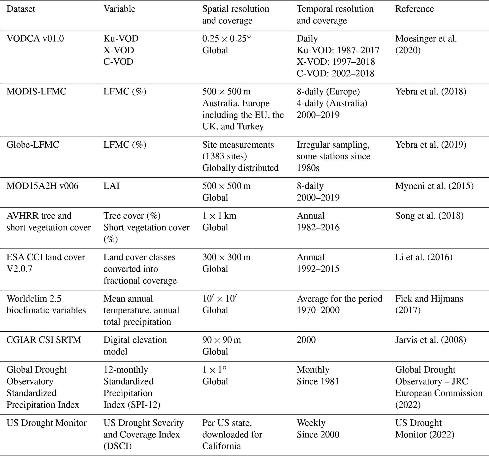
An overview of the properties of all used datasets is provided in Table 1.

Table 1 Properties of the used datasets.

2.1 Vegetation Optical Depth Climate Archive (VODCA) dataset

VOD was taken from the VODCA dataset (Moesinger et al., 2020). VODCA provides VOD at $\mathrm{0.25}{}^{\circ }\times \mathrm{0.25}{}^{\circ }$ spatial resolution in three separate wavelength bands with different temporal coverage, namely Ku-VOD (1987–2017), X-VOD (1997–2018), and C-VOD (2002–2018). The dataset is a merge of VOD retrievals from several passive microwave instruments that were derived with the Land Parameter Retrieval Model (LPRM) (Owe et al., 2001; van der Schalie et al., 2017). The merging uses a cumulative distribution function matching of the individual VOD retrievals into a joint long-term time series. Thereby VOD retrieved from the AMSR-E sensor is used as scaling reference (Moesinger et al., 2020).

The VODCA dataset has a daily temporal sampling, but observations are not available for each day dependent on time period and latitude. The VODCA dataset was masked for artefacts because of radio frequency interference (RFI), for land surface temperature < 0 ^∘C, and for negative VOD values, and therefore has mainly gaps in the winter months in northern latitudes. We did not perform any gap-filling or other further processing of the VODCA dataset. However, we excluded grid cells from further analysis that were either not vegetated or that have a higher coverage of ocean or inland water bodies (see Sect. 2.5).

Spatial patterns, seasonal dynamics, and long-term trends in the VODCA dataset have been intensively compared with datasets of leaf area index, gross primary production, and vegetation cover, and show that VODCA reflects common patterns of large-scale vegetation changes (Moesinger et al., 2020; X. Li et al., 2021; Wild et al., 2022).

2.2 Live fuel moisture content datasets

LFMC was taken from two datasets, namely from the Globe-LFMC database of site (Yebra et al., 2019) and from LFMC data retrieved from MODIS satellite observations by applying the methodology of Yebra et al. (2018) (in the following MODIS-LFMC). The Globe-LFMC measurements are the primary dataset for the comparison with VOD and to develop and calibrate the models to estimate LFMC from VOD. However, as there is severe scale mismatch between site measurements of LFMC and the coarse spatial resolution of VOD ($\mathrm{0.25}{}^{\circ }\times \mathrm{0.25}{}^{\circ }$), we additionally used LFMC retrievals from MODIS to make comparisons at the same spatial scale and to assess if the obtained results are comparable.

Globe-LFMC provides LFMC field measurements from 1383 sites in 11 countries, mainly in the USA (963 sites), China (229 sites), Spain (76 sites), and Australia (42 sites). However, each site has a different temporal coverage and sampling frequency of measurements, and different plant species are sampled (Yebra et al., 2019). For example, all sites in China have only one LFMC measurement, while the site “Reader Ranch” in California has 1291 measurements. At most sites, only one plant species is sampled throughout the time, but at other sites several plant species are sampled. LFMC values vary at many sites between species. In order to simplify the comparison of LFMC measurements from different species with VOD, we grouped each species according to their genus into a typical growth form. We considered the following growth forms: broad-leaved trees (TreeB), needle-leaved trees (TreeN), shrubs, grass (i.e. herbaceous graminoid), and forbs (i.e. herbaceous non-graminoid). As some plant genera can grow as tree or shrub, we decided for one or the other based on the land cover type (forest or shrubland) at the site and based on the site photos that come with the Globe-LFMC database.

MODIS-LFMC is based on an inversion (using look-up tables) of different radiative transfer models for grass/shrubs (PROSAILH) and trees (PROGeoSAIL) to estimate LFMC from surface reflectance observations of MODIS (Yebra et al., 2018). The method and dataset were initially developed for Australia. Additionally, we used retrievals for Europe based on the same method. The dataset provides LFMC at 500 m spatial resolution for the period 2000 to 2019 at 4-daily (Australia) and 8-daily (Europe) time steps. The dataset comes in tiles based on the original sinusoidal grid of MODIS observations. We first merged all tiles within Europe or Australia and then reprojected the data to a longitude/latitude projection (WGS84) using nearest neighbour resampling in Geospatial Data Abstraction Library software. We then aggregated the dataset to $\mathrm{0.25}{}^{\circ }\times \mathrm{0.25}{}^{\circ }$ spatial resolution of the VODCA dataset using spatial averaging.

2.3 Leaf area index – MODIS

As the relationship between VOD and LFMC also depends on leaf or canopy biomass, we additionally used leaf area index (LAI) retrievals from MODIS as a proxy for total leaf biomass. The MOD15A2H collection 6 product provides LAI globally on 500 m spatial resolution and 8-daily time steps (Myneni et al., 2015). We only used retrievals that were flagged as good quality in the dataset. Like the MODIS-LFMC data, the LAI data were projected to geographical coordinates and then aggregated to $\mathrm{0.25}{}^{\circ }\times \mathrm{0.25}{}^{\circ }$ spatial resolution by spatial averaging. The 8-daily MODIS LAI data obtain a clear temporal variability within months, which, despite the use of good quality observations, might be still related to atmospheric effects or possibly other changes in leaf and canopy properties (e.g. water content) that were not considered during the retrieval of LAI. As we here intend to use LAI only as a proxy for the temporal changes in canopy biomass, we averaged the 8-daily LAI values to monthly values to suppress the intra-monthly variability.

2.4 Vegetation cover and ancillary data

The cover of trees and short vegetation was used to stratify the comparison between LFMC and VOD with land cover information and to account for land cover in the models to calculate LFMC from VOD. For this purpose, we used the dataset from Song et al. (2018), which provides the percentage of tree cover, short vegetation, and bare ground within grid cells of 1 km × 1 km resolution. The dataset was estimated based on observations from Advanced Very-High-Resolution Radiometer (AVHRR) satellite sensors and provides annual maps for the years 1982 to 2016.

We additionally used information about ocean and inland water cover from the ESA CCI land cover map (version 2.0.7) (Li et al., 2016). We aggregated the land cover information from the original spatial resolution to the fractional coverage of different plant functional types at $\mathrm{0.25}{}^{\circ }\times \mathrm{0.25}{}^{\circ }$ by using the cross-walking approach (Poulter et al., 2015). We then used the fractional cover of water (>50 %) in grid cells to mask VOD data in global analyses (see Sect. 2.5).

Global maps of mean annual temperature and annual precipitation from the Worldclim 2.5 dataset (Fick and Hijmans, 2017) and the CGIAR SRTM digital elevation model (Jarvis et al., 2008) were used to stratify analyses with ancillary information (Fig. A4).

Time series of the 12-monthly Standardized Precipitation Index (SPI-12) and the US Drought Severity and Coverage Index (DSCI) were used in a case study to compare the large-scale estimates of LFMC with drought conditions in the western United States and in California. SPI-12 data were taken from the Global Drought Observatory (Global Drought Observatory – JRC European Commission, 2022) and DSCI data from the US Drought Monitor (2022).

2.5 Combination and comparisons of VOD and LFMC data

We combined the VOD and LFMC data in four different data combinations for our comparisons. Each combination of VOD and LFMC data had a different purpose and used a different masking or temporal sampling of data. The four combinations enable to: (1) compare satellite retrievals from MODIS-LFMC with the different bands of VOD; (2) compare site measurements of LFMC from Globe-LFMC with VOD; (3) calibrate and test models to estimate LFMC from VOD using LFMC site measurements; and (4) apply the best performing model to global VOD data to estimate LFMC globally.

The first data combination (D1) uses MODIS-LFMC for Australia and Europe to compare the temporal dynamic of LFMC with Ku-, X-, and C-VOD. In order to make a comparison of VOD and LFMC time series per grid cell and to assess the differences between the different VOD wavelengths, we only used observations from dates that occur in all four datasets (i.e. MODIS-LFMC, Ku-VOD, X-VOD, and C-VOD). These are for Australia 1390 time steps between 22 June 2002 and 28 July 2017, and for Europe 900 time steps between 26 June 2002 and 31 July 2017. We then computed the Spearman rank correlation between LFMC and the different VOD bands per grid cell and stratified the result for tree and short vegetation cover.

The second data combination (D2) is used to compare site measurements from Globe-LFMC with VOD. For this comparison, we used VOD data from the same days when LFMC measurements were available. As each site has a different temporal sampling of LFMC, the number of joint pairs of LFMC and VOD observations is on average per site 80, 72, and 42 for Ku-, X-, and C-VOD, respectively, whereby the differences between the number of observations for each band are caused by the longer temporal coverage of Ku-VOD than for X- or C-VOD. Single sites have up to 827 pairs of Ku-VOD/LFMC observations. For this comparison, we only matched LFMC with the dates of each individual VOD band, but did not match additionally the dates of the three VOD bands because this would decrease the availability of LFMC/VOD pairs further. We then computed the Spearman rank correlation between VOD and all LFMC measurements for each site (regardless of the sampled plant species) and also for each individual species at a site. We calculated the correlation for all sites/site-species with at least 10 pairs of LFMC/VOD observations. Based on this criterion, correlations were computed for 910 sites. We then assessed how a difference in the land cover distribution at the site and at the corresponding $\mathrm{0.25}{}^{\circ }\times \mathrm{0.25}{}^{\circ }$ grid cell affects the correlation between LFMC and VOD. Therefore, we extracted for the coordinate of each site the percentage of tree and short vegetation cover from the original resolution (1 km × 1 km) and the aggregated resolution ($\mathrm{0.25}{}^{\circ }\times \mathrm{0.25}{}^{\circ }$) of the vegetation cover dataset. The use of both resolutions allows assessing if the local land cover distribution at the site is comparable with the land cover distribution of the $\mathrm{0.25}{}^{\circ }\times \mathrm{0.25}{}^{\circ }$ grid cell of the VOD data. The difference in land cover between the 1 km spatial resolution at the local site and the coarse 0.25^∘ resolution of the corresponding grid cell was computed based on the Euclidean distance:

$$\begin{array}{}\text{(3)}& D=\sqrt{{\left({\mathrm{TC}}_{\mathrm{25}}-{\mathrm{TC}}_{\mathrm{1}}\right)}^{\mathrm{2}}+{\left({\mathrm{SV}}_{\mathrm{25}}-{\mathrm{SV}}_{\mathrm{1}}\right)}^{\mathrm{2}}},\end{array}$$

whereby TC and SV are tree cover and short vegetation, respectively, and the subscripts 1 and 25 denote the 1 km and 0.25^∘ spatial resolution. As TC and SV are percentages, the difference D is in percent.

The third data combination (D3) used Globe-LFMC site measurements to calibrate and evaluate models to estimate LFMC from VOD. We found from data combination D2 that the correlation between site measurements of LFMC and VOD decreases if the land cover distribution at 1×1 km around the site increasingly differs from the land cover distribution at the $\mathrm{0.25}{}^{\circ }\times \mathrm{0.25}{}^{\circ }$ grid cell of the VOD data (see results in Sect. 3.1). Therefore, we aimed to select only sites for the calibration and evaluation of models that are homogenous and representative for the coarse resolution of the VOD data. The Globe-LFMC database provides for each site a spatial coefficient of variation of the normalized difference vegetation index to quantify the homogeneity of vegetation cover at each site (Yebra et al., 2019). We used sites with a low coefficient of variation (CV < 0.26). Additionally, we used the land cover difference D (Eq. 3) to quantify the representativeness of the land cover at the site for the coarse spatial resolution of the VOD data. We selected only sites with D<10 %, i.e. with a similar land cover distribution at 1 km and 0.25^∘ spatial resolution. We further selected sites for model calibration that have at least 15 pairs of VOD and LFMC observations and that showed a positive correlation (r>0.2) between VOD and LFMC. These selection criteria left 216 combinations of sites and plant species at 163 sites to calibrate and test models (Fig. A4).

The fourth data combination (D4) uses daily-sampled VODCA Ku-VOD and monthly-averaged MODIS LAI to estimate daily LFMC globally with the best performing model for the overlapping period of both datasets (1 February 2000 to 31 July 2017). We applied the model to all grid cells at $\mathrm{0.25}{}^{\circ }\times \mathrm{0.25}{}^{\circ }$ spatial resolution that have on average at least 5 % vegetation cover (TC + SV ≥ 5 %) and that have less than 50 % water cover.

2.6 Models to estimate LFMC from VOD

We developed and tested four different models to estimate daily LFMC from daily values of VOD. All models were developed in this study either by assuming non-linear regressions between LFMC and VOD or by adopting known relations between LFMC, VOD, VWC, and dry biomass from previous studies (Jackson and Schmugge, 1991; Sawada et al., 2016; Frappart et al., 2020). Specifically, in models A and B we assume a positive relationship between VOD and LFMC and use logistic regression (S-shaped curve) to estimate LFMC from VOD. We use logistic regression because LFMC cannot be smaller than 0 % and LFMC values higher than 200 % are rare (the 95th percentile of LFMC is 193 %, the maximum is 549 % in the Globe-LFMC database). In models C and D, we adopt the relationships between LFMC, VWC, and dry biomass (Eq. 1) and between VOD and VWC (Eq. 2) to calculate LFMC. The four models are described with more detail in the following paragraphs. Each model has up to four model parameters. Prior ranges and values of those model parameters were manually selected in order to always obtain a positive relationship between VOD and LFMC and to obtain typical LFMC values (Table 2).

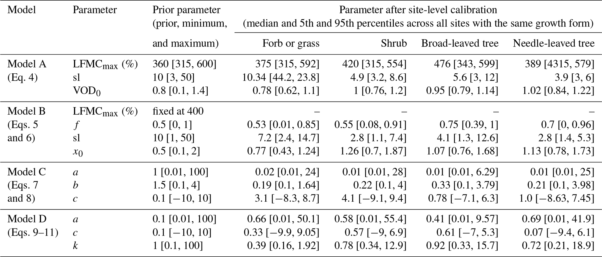
Table 2 Overview about prior parameter values and results after site-level calibration for the four models.

In Model A, we assume that LFMC is directly proportional to VOD by using a logistic regression as follows:

$$\begin{array}{}\text{(4)}& \mathrm{LFMC}={\displaystyle \frac{{\mathrm{LFMC}}_{\max }}{\mathrm{1}+e^{-\mathrm{sl}\times \left(\mathrm{VOD}-{\mathrm{VOD}}_{\mathrm{0}}\right)}}},\end{array}$$

where LFMC_max is the maximum possible LFMC value (in %) and sl is the slope of the curve. VOD₀ is the inflection point of the logistic curve, i.e. the VOD value at which half of the LFMC between 0 % and LFMC_max is reached. The parameters LFMC_max, sl, and VOD₀ were calibrated for each site.

In Model B, we additionally assume that LFMC depends on seasonal changes in canopy structure. Therefore, we additionally include monthly-averaged LAI as predictor. We assume that LFMC can be expressed based on a weighted combination x of daily VOD and monthly-averaged LAI. Like in Model A, we use a logistic regression in order to limit LFMC between 0 % and LFMC_max:

$$\begin{array}{}\text{(5)}& {\displaystyle }& {\displaystyle }x=f\times \mathrm{VOD}+(\mathrm{1}-f)\times \mathrm{LAI}\text{(6)}& {\displaystyle }& {\displaystyle }\mathrm{LFMC}={\displaystyle \frac{{\mathrm{LFMC}}_{\max }}{\mathrm{1}+e^{-\mathrm{sl}\times \left(x-x_{\mathrm{0}}\right)}}},\end{array}$$

where f is a fraction between zero and 1 that regulates if VOD (f=1) or LAI (f=0) contributes more to the calculation of x and hence to LFMC. Sl and x₀ are the slope and inflection point of the logistic curve. Note that we kept the parameter LFMC_max constant at 400 % in Model B (corresponding to the 99.99th percentile of LFMC in the Globe-LFMC database) throughout all analyses because the calibration results from Model A have shown that any high value for LFMC_max is not sensitive for the performance of the estimated LFMC.

For Model C, we directly made use of the VOD–LFMC relationship presented in Eq. (2) (Jackson and Schmugge, 1991; Konings et al., 2019) and compute LFMC by solving this equation for LFMC:

$$\begin{array}{}\text{(7)}& \mathrm{LFMC}={\displaystyle \frac{\mathrm{VOD}}{b\times m_{\mathrm{dry}}}}\times \mathrm{100}\mathit{\%}.\end{array}$$

To account for dry biomass of the canopy, we assume a linear relation with monthly-averaged LAI:

$$\begin{array}{}\text{(8)}& m_{\mathrm{dry}}=a\times \mathrm{LAI}+c.\end{array}$$

For the parameter b in Eq. (7), a prior value of 1.5 with a range between 0.1 and 4 was taken based on the values presented in Jackson and Schmugge (1991). The parameter a was varied between 0.01 and 100, as dry canopy biomass should positively scale with LAI. The parameter c is the intercept of this linear regression and was chosen around zero (between −10 and 10). Note that the parameters a and b are directly positively correlated in Model C and could indeed be represented by a combined product. However, as we have both prior information on the values of b (i.e. VOD–VWC relation) and a (i.e. the relation between leaf mass and leaf area) but not on their combined product, we decided to keep the two factors separated.

We developed Model D by using the basic definition of FMC (Eq. 1) and compute LFMC as the ratio between VWC and dry biomass:

$$\begin{array}{}\text{(9)}& \mathrm{LFMC}={\displaystyle \frac{\mathrm{VWC}}{m_{\mathrm{dry}}}}\times \mathrm{100}\mathit{\%}.\end{array}$$

Thereby, we compute VWC based on a exponential relationship between LAI and VWC (Paloscia and Pampaloni, 1988; Sawada et al., 2016) and compute dry biomass by assuming a positive relationship between VOD and biomass (e.g. Frappart et al., 2020). Following Sawada et al. (2016), VWC is computed based on an exponential relationship with LAI:

$$\begin{array}{}\text{(10)}& \mathrm{VWC}=e^{\frac{\mathrm{LAI}}{k}}-\mathrm{1},\end{array}$$

where the parameter k defines the shape of the exponential relationship. As we have no prior information about the value of k, we sampled k over a large range (0.1–100). The computation of dry biomass is based on a linear relation with VOD, which is based on the assumption that VOD at short wavelengths is proportional to canopy biomass (Frappart et al., 2020):

$$\begin{array}{}\text{(11)}& m_{\mathrm{dry}}=a\times \mathrm{VOD}+c.\end{array}$$

The parameters a and c define the relation with dry biomass like in Model C.

2.7 Site-level calibration and evaluation

The parameters of the models A to D were calibrated separately for each species at each site from the data combination D3. For the calibration, we used a genetic optimization algorithm together with a cost function that is sensitive to the statistical distribution of LFMC and the temporal correlation. We initially tested several common model performance measures as cost functions, like the root mean squared error (RMSE), modelling efficiency, and the Kling–Gupta efficiency (KGE) (Gupta et al., 2009), to calibrate the model parameters, but we found that based on those cost functions the variance of the observed LFMC was underestimated in most cases. As an alternative, we developed a cost function that aims to fit the observed variance by minimizing the differences in the percentiles of the statistical distribution of LFMC. The used cost function J adopts the basic definition of the Euclidean distance like in the Kling–Gupta efficiency, and is here defined as the Euclidean distance in a multivariate space of performance measures based on the Pearson correlation r between estimated and observed LFMC and the ratios of the 5th, 50th, and 95th percentiles p:

$$\begin{array}{}\text{(12)}& \begin{array}{rl}& J=\\ & \sqrt{\mathrm{3}\times (r-\mathrm{1}{)}^{\mathrm{2}}+{\left({\displaystyle \frac{S_{\mathrm{p}=\mathrm{5}}}{O_{\mathrm{p}=\mathrm{5}}}}-\mathrm{1}\right)}^{\mathrm{2}}+{\left({\displaystyle \frac{S_{\mathrm{p}=\mathrm{50}}}{O_{\mathrm{p}=\mathrm{50}}}}-\mathrm{1}\right)}^{\mathrm{2}}+{\left({\displaystyle \frac{S_{\mathrm{p}=\mathrm{95}}}{O_{\mathrm{p}=\mathrm{95}}}}-\mathrm{1}\right)}^{\mathrm{2}}},\end{array}\end{array}$$

where S and O are the percentiles of simulated and observed LFMC, respectively. The individual terms in the cost function are zero in case of a perfect model–data agreement and can go to infinite. The correlation-related term was multiplied with 3 to give the temporal correlation the same weight like the three distribution-based ratios.

The cost function was minimized for each model and for each plant species at each site by using the Genetic Optimization using Derivatives (GENOUD) algorithm (R package rgenoud, version 5.8-3) (Mebane and Sekhon, 2011). GENOUD is a global optimization algorithm that additionally uses a local search algorithm. We used GENOUD with 100 parameter sets per generation and computed it for 10 generations. The local search algorithm was used only after the third generation to avoid a too fast convergence of the algorithm to a local minimum. Prior ranges of each parameter (Table 2) were provided as search domains to the optimization algorithm. As a measure for parameter uncertainty, we then selected the best-performing parameter sets from the optimization results, which have a cost J less than or equal to the 25th percentile of all parameter sets in an optimization run. As a result, we obtained for each species at each site a sample of best-performing parameters for each model. The median and the 5th and 95th percentiles of each parameter from the best-performing parameter sets are listed for different growth forms in Table 2.

Additionally to the used cost function, we used the Pearson correlation coefficient r, the RMSE, and the KGE performance measures to evaluate the optimization results. The KGE allows associating the lack of model performance to a mismatch between observed and estimated mean values (bias component), to a mismatch between observed and estimated variance (variance component) and to a lack of correlation (correlation component) (Gupta et al., 2009). We used the KGE and its three components to diagnose the model performance.

Please note that we did not perform for the site-level calibrations any evaluation with independent test data. We used at each site all available pairs of LFMC/VOD observations for model calibration, because a split of the available LFMC observations would further reduce the available data and sites for model calibration as many sites have few observations. However, we built a random forest model to predict the parameters of the best-performing model in space and we applied spatial cross-validation to evaluate the performance of the predicted LFMC (Sect. 2.8).

2.8 Spatial model application, evaluation, and uncertainty assessment

The calibration of model parameters was performed for each species at each site, and allows evaluating and comparing the performance of the four models at site level. However, in order to apply the best-performing model globally, the model parameters need to be estimated for each grid cell of the global $\mathrm{0.25}{}^{\circ }\times \mathrm{0.25}{}^{\circ }$ raster. We therefore tested different regression approaches to predict single model parameters from percentage tree cover or from other model parameters. We initially tested different regression approaches to estimate the model parameters, namely linear regression, second- and third-order polynomials, generalized additive models (GAMs), and random forest (RF). While third-order polynomials, GAM, and RF resulted in similar performance in training, only RF had plausible results in cross-validation. Hence, we decided to use RF to estimate the parameters of Model B in space. Thereby, we followed a step-wise application of RF: in the first RF model, we predicted the parameter x₀ of Model B from percentage tree cover. In the second RF model, we then predicted the parameter sl from tree cover and the parameter x₀. In the third RF model, we predicted the parameter f from tree cover and the parameters x₀ and sl. The parameter LFMC_max was held constant at 400 %. We applied RF in the same way for the parameters of the other models by first always predicting the parameter that had the highest correlation with tree cover. We used the randomForest package version 4.6-14 (Liaw and Wiener, 2002) in R with 200 decision trees per RF and a node size of 15. A higher number of decision trees did not result in better performance. The node size describes the number of samples in the terminal nodes of each decision trees that are averaged to provide the regression result. Note that we here used based on our experience with RF a higher node size of 15 than the default value of 5 in order to reduce the risk of overfitting when using RF with only one to three predictors and only 216 sites. In summary, to predict the parameters of Model B for one grid cell, a nested set of three RF models is needed (one RF for each parameter).

In order to train and evaluate the set of three RF models, we applied a 20-fold spatial cross-validation procedure. Therefore, we spatially clustered all Globe-LFMC sites from the data collection D4 based on their coordinates using a k-means clustering with 20 clusters. We then used the optimized model parameters from all sites within 19 clusters to train the set of three RF models, and applied the trained set of RF to the 20th cluster to predict and evaluate the parameters of Model B. Model B was then applied with the predicted parameters to estimate LFMC and to cross-validate LFMC. The procedure was repeated 20 times so that once each spatial cluster was not included in the training of the RF models, it was rather used for cross-validation.

During this spatial training and cross-validation procedure, we also attempted to propagate the uncertainty of the optimized model parameters. Therefore, we randomly sampled from each Globe-LFMC site in the training set five out of the best-performing parameter sets from the site-level calibration. Hence, in each of the 20 folds, a different combination of best-performing parameter sets was used to train the set of RF models.

The spatial training and cross-validation resulted in 20 sets of RF models that allow estimating Model B parameters for any grid cell based on percentage tree cover. Each of the 20 sets of RF models varies based on the spatial distribution of the used Globe-LFMC sites in training and based on the uncertainty of the best-performing model parameters after site-level calibration. To estimate LFMC globally, we applied all 20 sets of RF models to all global vegetated grid cells. Therefore, we excluded grid cells with less than 5 % vegetation cover (tree cover + short vegetation cover) and grid cells with more than 50 % water cover. For each grid cell we then obtained the model parameters from the set of RF models and used Model B to predict 20 realisations of LFMC. We then computed from the predicted LFMC values the median, minimum, and maximum values as measures of the uncertainty. In the results, we display this uncertainty estimate as relative uncertainty (i.e. (maximum LFMC − minimum LFMC)$/$median LFMC).

2.9 Global random forest model as alternative to models A–D

As described in the previous section, we used RF to estimate parameters of models A–D in space and then apply those models to estimate LFMC. As an alternative, RF could be used directly to estimate LFMC globally, which would not require any assumptions about the type of relationships like in models A–D and allows a higher flexibility in including predictor variables. In order to assess the performance of the spatially-applied models A–D against a more flexible global RF model, we trained a global RF model directly against LFMC measurements from all sites within the 20 spatial folds and by using the same set of predictors that we used for Model B (i.e. daily Ku-VOD, monthly LAI, and tree cover). The global training of the RF was performed with the same spatial cross-validation procedure like for the other models, i.e. with the same set of 20 folds of spatially-clustered LFMC sites.

3 Results and discussion

3.1 Correlation between VOD and LFMC

3.1.1 Temporal and spatial correlations

The comparison of VOD and LFMC time series from ground measurements and MODIS retrievals shows widespread positive temporal correlations (Fig. 1). Across the 910 Globe-LFMC sites with ≥10 pairs of VOD/LFMC observations, the median temporal correlation between LFMC and VOD is 0.10 for Ku- and X-VOD and 0.06 for C-VOD. The maximum correlation is 0.88 for Ku-VOD, 0.79 for X-VOD, and 0.80 for C-VOD. Globally, 633 sites show positive correlations and 277 sites show negative correlations with Ku-VOD. For X- and C-VOD, 632 and 395 sites show positive correlations, respectively. The comparison with MODIS-LFMC shows median correlations of 0.30 for Ku-VOD, 0.26 for X-VOD, and 0.28 for C-VOD in Europe and 0.39 for Ku-VOD, 0.37 for X-VOD, and 0.35 for C-VOD in Australia. These results show that correlations between VOD and LFMC from site measurements and MODIS retrievals are in the majority of sites or grid cells positive and similar for the different VOD bands, but that Ku-VOD shows slightly higher correlations.

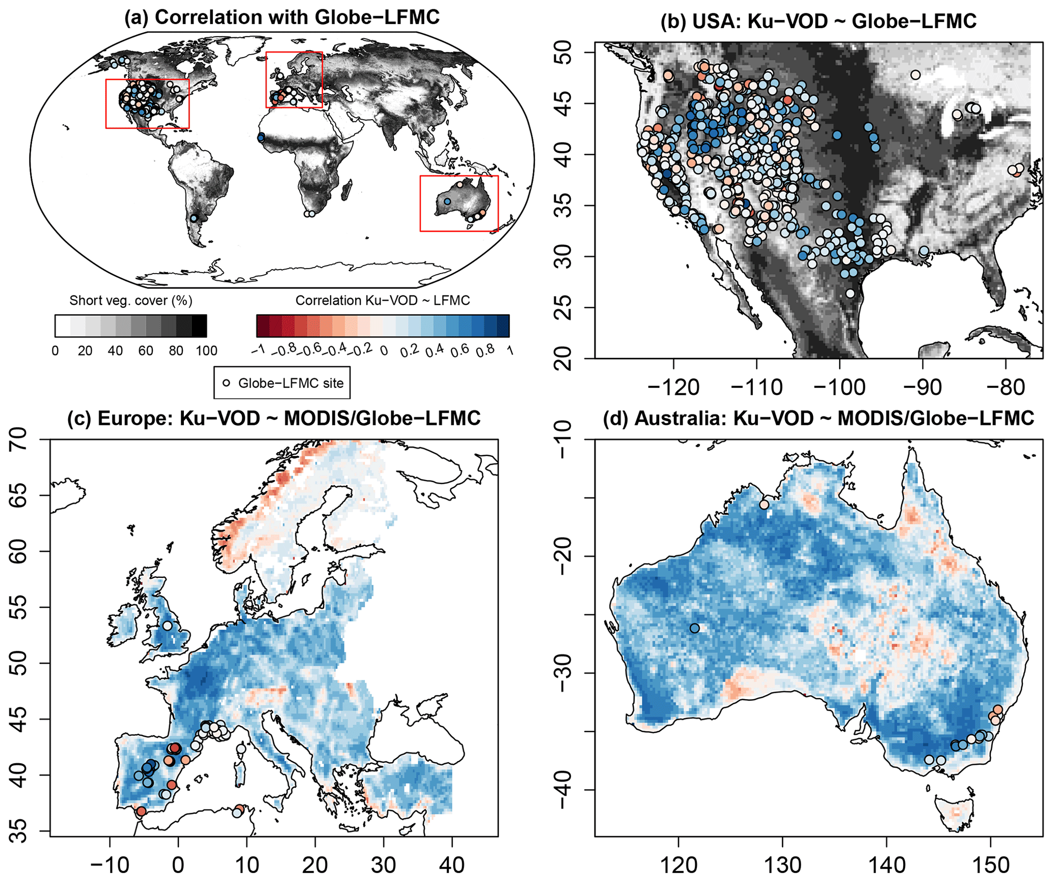
Figure 1 Temporal correlations between Ku-VOD and LFMC. Correlations of Ku-VOD with Globe-LFMC sites are plotted as point symbols and with MODIS-LFMC as coloured back ground raster (in c and d). The greyscale raster in (a) and (b) shows percentage of short vegetation cover.

The spatial pattern of temporal correlations between LFMC and Ku-VOD indicate spatial clusters with medium to high positive correlation and clusters with low or negative correlation (Fig. 1). In the USA, sites with low correlation (r<0.1) are in many cases distributed along the mountain ranges of the Rocky Mountains, Coast Range, or Sierra Nevada (Fig. 1b). This association of low correlations with mountain ranges is also confirmed by the comparison with MODIS-LFMC in Europe, where positive correlations between LFMC and Ku-VOD are widespread, but negative correlations occur in the Alps, the Carpathians, and the Scandinavian mountains (Fig. 1c). Additionally, the flatter areas of central and eastern Scandinavia show generally very low correlations between Ku-VOD and MODIS-LFMC. In Australia, positive correlations between LFMC and Ku-VOD dominate, but negative correlations occur in parts of the northern Great Dividing Range and in parts of the Simpson Desert and the Nullabor Plain (Fig. 1d). These spatial patterns of correlations with MODIS-LFMC are nearly identical in all three VOD bands.

All global spatio-temporal pairs of VOD and LFMC site measurements together show a weak positive correlation but a large bi-variate scatter (Fig. 2a–c). This scatter between globally distributed VOD and LFMC indicates that a unique global VOD–LFMC relation does not exist, or that such a relationship is modified by other surface and land cover properties or by the scale mismatch between VOD grid cells and LFMC site measurements.

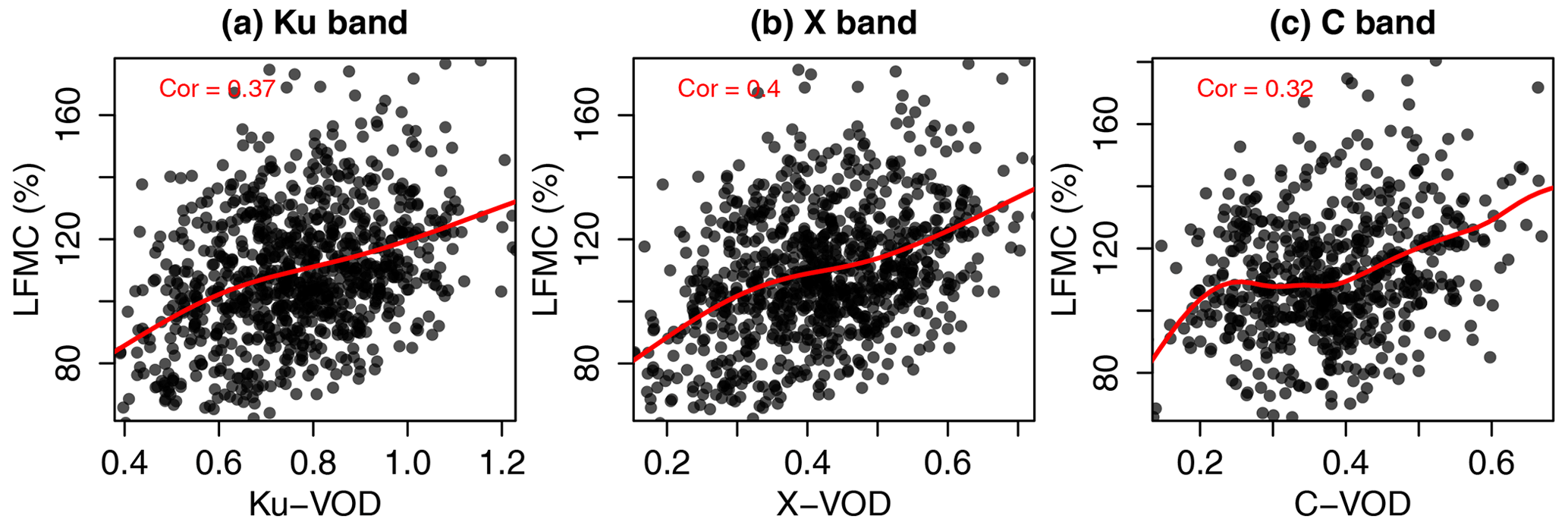
Figure 2 Global scatterplots and correlation of LFMC from the Globe-LFMC database against Ku-, X-, and C-VOD. The red lines are smoothing spline fits between the values at the x and y axes.

The medium to high positive correlations between VOD and LFMC in the majority of sites support earlier studies that identified a relationship between VOD and VWC or LFMC (Jackson and Schmugge, 1991; Konings et al., 2019). Despite the strong similarity in correlations between LFMC and the different VOD bands, contaminations by residual effects of RFI could explain the slightly lower correlation for C-VOD. The VODCA dataset uses the RFI flagging in LPRM version 6.0, which is based on the method proposed by de Nijs et al. (2015). Main contamination areas in AMSR2 in both the C1- (6.9 GHz) and C2- (7.3 GHz) bands include North America and Europe (de Nijs et al., 2015), where the majority of Globe-LFMC sites is also located. We observed that some residual RFI can still be observed in these areas, which was not covered by the masking used in VODCA (Fig. A1). As the D2 data combination uses VOD from the same days as Globe-LFMC without any smoothing, it is likely that the lower correlation between C-VOD and LFMC is affected by residual RFI.

3.1.2 Effect of land cover differences between scales

The site measurements of LFMC and the $\mathrm{0.25}{}^{\circ }\times \mathrm{0.25}{}^{\circ }$ grid cells of the VOD data are representative for very different scales. Therefore, we further investigated how a difference in land cover at a site (here defined as the 1 km grid cell in which the site is located) and at the 0.25^∘ grid cell affects the temporal correlations between LFMC and VOD. Despite a large variability of temporal correlations, on average we found decreasing correlations with increasing dissimilarity in land cover distribution between the site-scale and the VOD grid. For example, the correlation between Globe-LFMC and Ku-VOD increased by 0.07 (to median r=0.17) if the land cover difference is less than 10 %. In this case, 126 sites had negative correlations and 365 sites had positive correlations. Hence, the difference in land cover at an LFMC measurement site and in the coarse VOD grid cell can explain a small decrease in the correlation between VOD and LFMC.

Although this analysis allowed to quantify how the correlation between site measurements of LFMC and coarse-resolution grid cells of VOD are affected by the land cover differences between both scales, it does not allow to resolve this scale mismatch. Only local measurements of passive microwave emissions and derived estimates of VOD in conjunction with LFMC samples allow to factor out the scale mismatch for the analysis of relations between LFMC and VOD. However, such measurements are rare (Momen et al., 2017). Our results demonstrate the need to better understand the effect of the local to regional heterogeneity in land cover on coarse-scale VOD estimates in order to make better use of VOD in estimating LFMC.

3.1.3 Effect of vegetation type

Furthermore, we investigated if the correlations between VOD and LFMC are associated to vegetation type (Fig. 3). The comparison of VOD with Globe-LFMC shows higher correlations at higher short vegetation cover within the VOD grid cell. For example, the median correlation between LFMC and Ku-VOD is 0.30 if the short vegetation cover is ≥80 % and is 0.09 if the short vegetation cover is <80 % (Fig. 3a). However, despite this average increase in correlation with increasing short vegetation cover, several sites with low short vegetation cover also have correlations of  > 0.5. The increase of correlation with short vegetation cover is mirrored by a decrease of correlation with increasing tree cover. For example, the median correlation between Globe-LFMC and Ku-VOD is 0.15 for tree cover < 20 % and is 0.05 for tree cover ≥ 20 %. The changes in correlation with short vegetation or tree cover are similar for all three VOD bands, but Ku-VOD shows in the majority of vegetation cover fractions higher correlations than the other two bands. The dependency of the correlation between LFMC and VOD on vegetation type is more pronounced if we use MODIS-LFMC instead of Globe-LFMC site measurements. Thereby, we find for all VOD bands and both in Australia and Europe a general increase of the correlation with increasing short vegetation cover (or decreasing tree cover) (Fig. 3c and d).

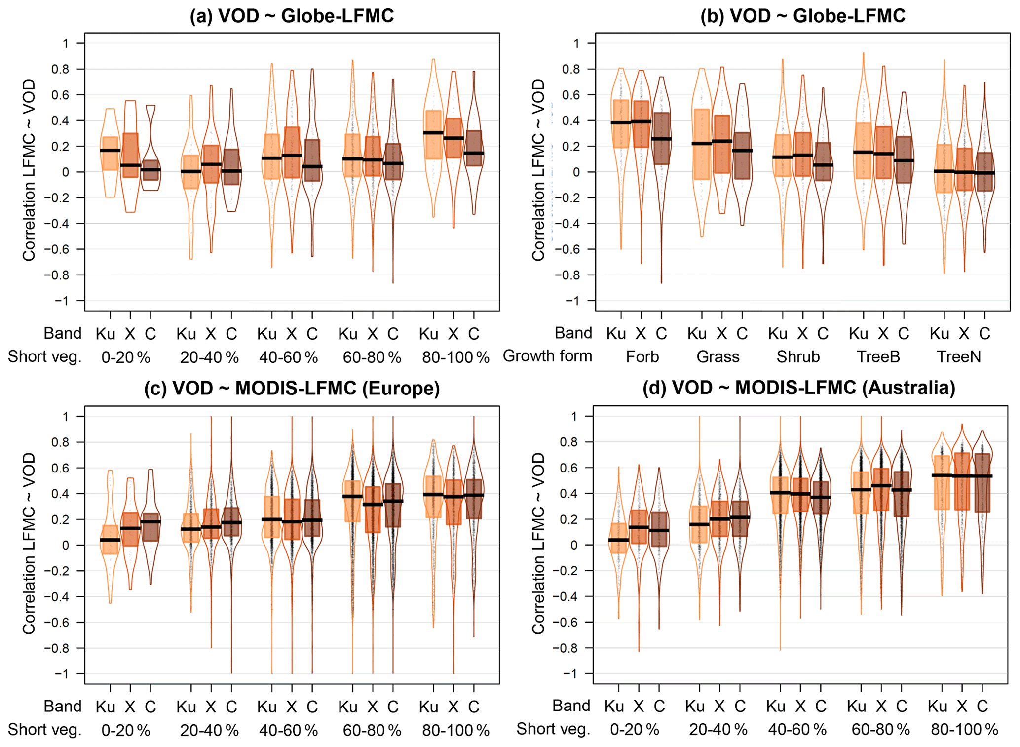
Figure 3 Statistical distributions of the temporal correlation between VOD and LFMC stratified by vegetation type. (a, b) Correlation with measurements from the Globe-LFMC database stratified by (a) the percentage cover of short vegetation and (b) by the growth form of the sampled plant. (c, d) Correlation with MODIS-LFMC in (c) Australia and (d) Europe stratified by the percentage cover of short vegetation.

The dependency on vegetation composition becomes clearer when we compute the correlation between VOD and LFMC separately for each sampled plant species at each site and then grouped the plant species in growth forms (Fig. 3b). We find the highest correlation for forbs (median r=0.38 for Ku-VOD), followed by grass (r=0.22), broad-leaved trees (r=0.15), shrubs (r=0.11), and finally needle-leaved trees (r=0). The order of median correlations is the same for X- and C-VOD. However, the results show that despite low median correlations for some growth form classes, high correlations are also possible at some sites for all growth forms. For example, the 90th percentile of the correlation between LFMC and Ku-VOD is 0.7 for forbs, 0.65 for grass, 0.55 for shrubs, 0.61 for broad-leaved trees, and 0.40 for needle-leaved trees. These results demonstrate that especially Ku-VOD is related to LFMC and that the relationship is closest for short vegetation types such as forbs, grasses, and shrubs.

The results are in agreement with earlier studies that established the relation between VOD and VWC or LFMC based on observations from crops and grasses (Jackson and Schmugge, 1991; Konings et al., 2019). The more homogenous canopies of short vegetation than of forest canopies might cause the generally higher correlations between VOD and LFMC at many herbaceous sites than at forest sites. However, based on the additional high 90th percentiles of correlations at some tree-dominated sites, we assume that coarse-resolution VOD data are also sensitive to LFMC at forest sites but that the relationship is in many cases masked by the mismatch between land cover at the local site and the coarse VOD grid cell. This assumption is also supported by the findings of Holtzman et al. (2021) who report a correlation of r=0.76 between L-VOD and leaf water potential as measured locally in a deciduous forest and by Momen et al. (2017) who were able to model X-VOD from measurements of leaf water potential and LAI for two mixed deciduous forests.

The higher correlation for Ku- and X-VOD with LFMC than for C-VOD might be confounded by an effect of rain on the atmospheric transmissivity of those wavelengths. Although microwaves are generally assumed largely independent of atmospheric conditions, thick water clouds and rain reduce the transmissivity of the atmosphere especially for shorter wavelength microwaves. For example, the atmospheric transmissivity is between 60 % and 80 % in the case of water clouds and between 20 % and 70 % in the case of rain for Ku-band (Ulaby et al., 1981, p. 2–3). However, effects of rain on the retrievals of Ku- and X-VOD in the VODCA product are not known. Overall, the quality of the Ku-band VOD is comparable to X- and C-VOD (Moesinger et al., 2020): Ku-VOD correlates higher (global average r=0.39) with MODIS LAI than C-VOD (r=0.37) but a bit weaker than X-VOD (r=0.42). The effect of RFI on C-VOD is not present in Ku-VOD. Moreover, Ku-VOD has a larger data coverage because the CDF matching approach used in the VODCA dataset was more often successful for Ku-VOD than for the X- or C-VOD data. Multi-year trends in Ku-VOD agree with trends in X and C-VOD. Hence, the higher correlation of Ku-VOD with LFMC and the quality and overall similarity of the Ku-VOD data with X- and C-VOD, suggests using Ku-VOD to estimate LFMC.

3.2 Estimating LFMC at site-level

3.2.1 Performance of models A–D in site-level calibration

Based on the finding that Ku-VOD shows slightly higher correlations with LFMC than X- or C-VOD and given the longer temporal overlap of Ku-VOD with Globe-LFMC observations, we used Ku-VOD as input to four different models to estimate LFMC. We separately calibrated each model at each of 216 Globe-LFMC sites that were selected based on the criteria for the data collection D3 (Sect. 2.5). An example of the calibration of Model B for one species at one site is shown in Fig. 4. The example demonstrates a very good fit between observed and estimated LFMC (correlation r=0.84). This example corresponds approximately to the 90th percentile highest correlation between observed and estimated LFMC from Model B and is therefore among the best results of all sites. The model response function shows that the estimated LFMC increases with both daily Ku-VOD and monthly LAI, which is supported by the observed LFMC (Fig. 4b). In this model, the performance of the estimated LFMC is most strongly influenced by the parameter sl (e.g. r=0.95 between sl and RMSE), while the parameter x₀ also has a strong effect on the model performance (e.g. $r=-\mathrm{0.65}$ between x₀ and RMSE). This example shows that LFMC from site-level observations can be estimated from coarse resolution Ku-VOD (and LAI) observations.

Figure 4 Example of the fit of Model B using daily Ku-VOD and monthly LAI for Artemisia tridentata ssp. at the site Great Divide, Colorado (40.76^∘ N, 107.85^∘ W). (a) Scatterplot of estimated against observed LFMC. (b) Distribution of observed LFMC (points) and estimated LFMC (coloured background) in relation to daily Ku-VOD and monthly LAI.

Across all sites and vegetation types, the estimated LFMC from Model B shows a better fit against the observed LFMC than the estimates from the other three models (Fig. 5). Model B achieves correlations of 0.64${}_{\mathrm{0.36}}^{\mathrm{0.86}}$ (median and 5th and 95th percentiles), followed by Model D with 0.54${}_{\mathrm{0.66}}^{\mathrm{0.83}}$, Model A with 0.45${}_{\mathrm{0.16}}^{\mathrm{0.75}}$, and finally Model C with 0.41${}_{\mathrm{0.06}}^{\mathrm{0.75}}$. Also for the RMSE, Model B shows the lowest error with RMSE = 29${}_{\mathrm{11.5}}^{\mathrm{60.7}}$ %-LFMC. The other three models show higher RMSE with Model C having the highest error (RMSE = 44.9${}_{\mathrm{10.1}}^{\mathrm{643}\mathrm{707}}$ %-LFMC). Please note the high 95th percentile of the RMSE for Model C, which indicates that it was not possible to successfully fit Model C at some sites.

Figure 5 Performance of the models A–D using daily Ku-VOD (and monthly LAI in models C and D) after calibrating each model at each site. Shown is the root mean squared error (RMSE) and correlation coefficient between estimated and measured LFMC. Small dots are results from different parameter sets at each site, and big dots and bars are the median and range from the 5th–95th percentiles across all sites, respectively.

By investigating the model performance for different vegetation growth forms, we generally found that Model B performed best and that the ranking of model performance for the other three models is similar for all vegetation types (Fig. 5). We found the highest correlation between estimated and observed LFMC for shrubs (0.73${}_{\mathrm{0.46}}^{\mathrm{0.87}}$, Model B), followed by forbs and grasses (0.67${}_{\mathrm{0.44}}^{\mathrm{0.83}}$), broad-leaved trees (0.55${}_{\mathrm{0.32}}^{\mathrm{0.86}}$), and needle-leaved trees (0.50${}_{\mathrm{0.28}}^{\mathrm{0.70}}$). The lowest median correlation was found for Model C for broad-leaved trees (0.35${}_{\mathrm{0.14}}^{\mathrm{0.62}}$). While the models A, B, and D resulted in only positive correlations between observed and estimated LFMC, Model C produced negative correlations at five sites. In terms of the RMSE, needle-leaved trees had the lowest error with RMSE = 15 %-LFMC (median for Model B), followed by shrubs (RMSE = 19 %), broad-leaved deciduous trees (RMSE = 35 %), and forbs and grasses (RMSE = 39 %). The results indicate that the performance of the models to estimate LFMC from Ku-VOD depends on vegetation type. Thereby, the temporal correlation can be well estimated for all vegetation types using Model B. The absolute values of estimated LFMC show low to medium errors for most vegetation types except for broad-leaved evergreen trees.

3.2.2 Suitability of model structures

The logistic regression Model B based on daily VOD and mean monthly LAI outperforms other model structures. The improved performance of Model B (using VOD and monthly LAI) over Model A (only using VOD) demonstrates that the dynamics in LAI need to be considered in order to provide good estimates of LFMC. The parameter f in Model B defines the relative contribution of VOD or LAI to the estimated LFMC. The higher values of f for trees than for grasses and forbs (Table 2) show that VOD needs to be higher weighted to predict the LFMC of forest sites, while a lower weight of VOD (and higher relative contribution of monthly LAI) is necessary to predict the LFMC of grasses and forbs. The higher weighting of VOD to predict LFMC of trees corresponds to the findings of Zhang et al. (2019) who found that canopy biomass has a stronger effect on short-wavelength VOD than leaf water potential in temperate forests.

Model C adapted the relationship between VOD and LFMC as proposed by Jackson and Schmugge (1991) and Konings et al. (2019) (i.e. Eq. 2). Hence, this model used VOD to account for VWC and used LAI to account for canopy biomass. Model C resulted on average in low correlations and high errors between estimated and observed LFMC. While this model could not be fitted successfully at some sites, it also reached good performances at others. These results suggest that the relationship between VOD and LFMC as denoted in Eq. (2) is valid for some sites but it might not be valid for all sites or is overly sensitive to scale mismatches in the local measurements and the coarse-scale VOD and LAI data.

Model D adapted the relationship between VWC and LAI as suggested by Sawada et al. (2016) and estimated canopy biomass based on VOD. As this model resulted in better performance than Model C, it indicates that VOD is indeed a valuable predictor for canopy biomass and VWC can be indeed estimated from LAI at many sites. Model D achieved on average higher correlations between estimated and observed LFMC than Model A (only using VOD), which shows that LAI is required to predict temporal dynamics in LFMC. However, Model D had higher errors than Model A, which indicates that using VOD only as predictor for canopy biomass is not sufficient but that the VOD information in Model A provides information of absolute values (and hence reduces errors) of LFMC.

Models A, C, and D with lower performance have a low flexibility in how they use VOD and LAI to estimate LFMC: Model A only uses VOD; Model C uses VOD to account for VWC and LAI to account for biomass; and Model D uses LAI to account for VWC and VOD to account for biomass. On the other hand, Model B allowed to combine daily VOD and monthly LAI in a flexible way to estimate LFMC and reached highest performance. These results demonstrate that flexible model structures are needed in order to estimate LFMC from VOD and LAI. This finding is supported by several studies that identified that the relative contributions of changes in biomass and vegetation water content (or leaf water potential) depends on land cover type (Momen et al., 2017; Zhang et al., 2019; Konings et al., 2021b).

3.3 Estimating LFMC spatially using spatial cross-validation

In a next step, we investigated the applicability of the four models in space, which requires an estimate of the model parameters for each of the 0.25^∘ VOD grid cells. Therefore, we first analysed the correlation of the estimated parameters of each model with land cover properties of the VOD grid cell (e.g. shown for Model B in Fig. A2). We found that some of the optimized model parameters are highly correlated with land cover information, while other parameters can be estimated based on the covariation between parameters. For example, in Model B the parameter x₀ had the strongest correlation with the percentage tree cover (r=0.74), the parameter sl with the parameter x₀ ($r=-\mathrm{0.74}$) and then with tree cover ($r=-\mathrm{0.32}$), and the parameter f with the parameter sl (r=0.3) (Fig. A2). Based on those findings, we used random forest to predict first for each VOD grid cell the parameter x₀ from percentage tree cover and then the parameter sl from tree cover and the parameter x₀. Finally, we predicted the parameter f from tree cover and the parameters x₀ and sl. We performed the same step-wise approach to predict the parameters with random forest for the other models and then applied each model to the 0.25^∘ grid cell by using the predicted parameters to estimate LFMC. We applied this approach within a 20-fold spatial cross-validation to evaluate the performance of the estimated LFMC in space. Additionally, we use RF to estimate the spatial–temporal dynamics of LFMC directly.

3.3.1 Model performance in spatial cross-validation

As expected, the performance of all models slightly decreased in cross-validation in comparison to the site-level calibration results (Fig. 6). However, the ranking in model performance remained the same with Model B showing the best performance. For example, Model B had correlations of 0.58${}_{\mathrm{0.30}}^{\mathrm{0.84}}$ in spatial cross-validation samples (0.64${}_{\mathrm{0.36}}^{\mathrm{0.86}}$ in site-level calibration, see Sect. 3.2), which corresponds to a decrease of 0.06 of the median correlation in comparison to the calibration against the site data. The RMSE in spatial cross-validation was 48.8${}_{\mathrm{17.9}}^{\mathrm{111.8}}$ %-LFMC for Model B (RMSE = 29${}_{\mathrm{11.5}}^{\mathrm{60.7}}$ %-LFMC in site-level calibration). Like Model B, models A and D also experienced small decreases in correlation and increases in RMSE in spatial cross-validation (Fig. 6). However, Model C experienced strong decreases in correlation from median r=0.42 in site-level calibration to r=0.22 in spatial cross-validation, which shows the parameters of Model C could not be reliably estimated in space in order to obtain a sufficient performance in estimating LFMC.

Figure 6 Performance of the models A–D using Ku-VOD after calibrating each model for each species at each site (cal at site) and after using sites as test data in spatial cross-validation after the application of random forest to predict model parameters (spatial-cv). The global RF model (shown in orange) was directly trained against LFMC measurements from multiple sites. Shown is the root mean squared error (RMSE) and correlation coefficient between estimated and measured LFMC. Dots and bars are the median and range from the 5th–95th percentiles across all sites, respectively.

The global RF model achieved comparable performances like the other models, with correlations of 0.50${}_{\mathrm{0.18}}^{\mathrm{0.77}}$ and RMSE of 40${}_{\mathrm{21.9}}^{\mathrm{79.5}}$ %-LFMC in spatial cross-validation between observed and estimated LFMC. Hence, the RF performed on average slightly better than the best-performing Model B in terms of RMSE, but worse than models B and D in terms of correlation.

These results demonstrate that especially Model B can be applied in space and results in a comparable performance in estimated LFMC between site-level calibration and spatial cross-validation.

We then performed a more detailed evaluation of the cross-validation results of the best-performing Model B by investigating the Kling–Gupta efficiency (KGE) and its components for each site and each vegetation growth form (Fig. 7). We found the highest KGE in cross-validation for shrubs (median KGE = 0.4) and forbs (median KGE = 0.32). Grasslands (median KGE = 0.29) and broad-leaved trees (median KGE = 0.25) had lower performance and needle-leaved trees had overall low performance (median KGE = −0.49). However, the variability in KGE was high within all vegetation types. All grass sites and 88 % of the forb and shrub sites had positive KGE, but only 38 % of the needle-leaved sites had positive KGE. In most sites with low KGE, KGE is dominated by a mismatch between the observed and estimated variance of LFMC. This can be seen for example in the LFMC time series in Fig. 7b, which is representative for a broad-leaved tree site with low KGE and corresponds to the 5th percentile of the KGE across all sites. However, the correlation between observed and estimated LFMC is still moderate at such sites, which indicates that the temporal dynamic of the estimated LFMC has still a moderate agreement with the observed LFMC. For sites with medium and high KGE (Fig. 7c and d), the error is in most cases a mixture of a mismatch in mean values (bias), variance, or not-perfect correlation. For example, the time series in Fig. 7c and d demonstrates that Model B fits well the mean, variance. and correlation of the observed LFMC.

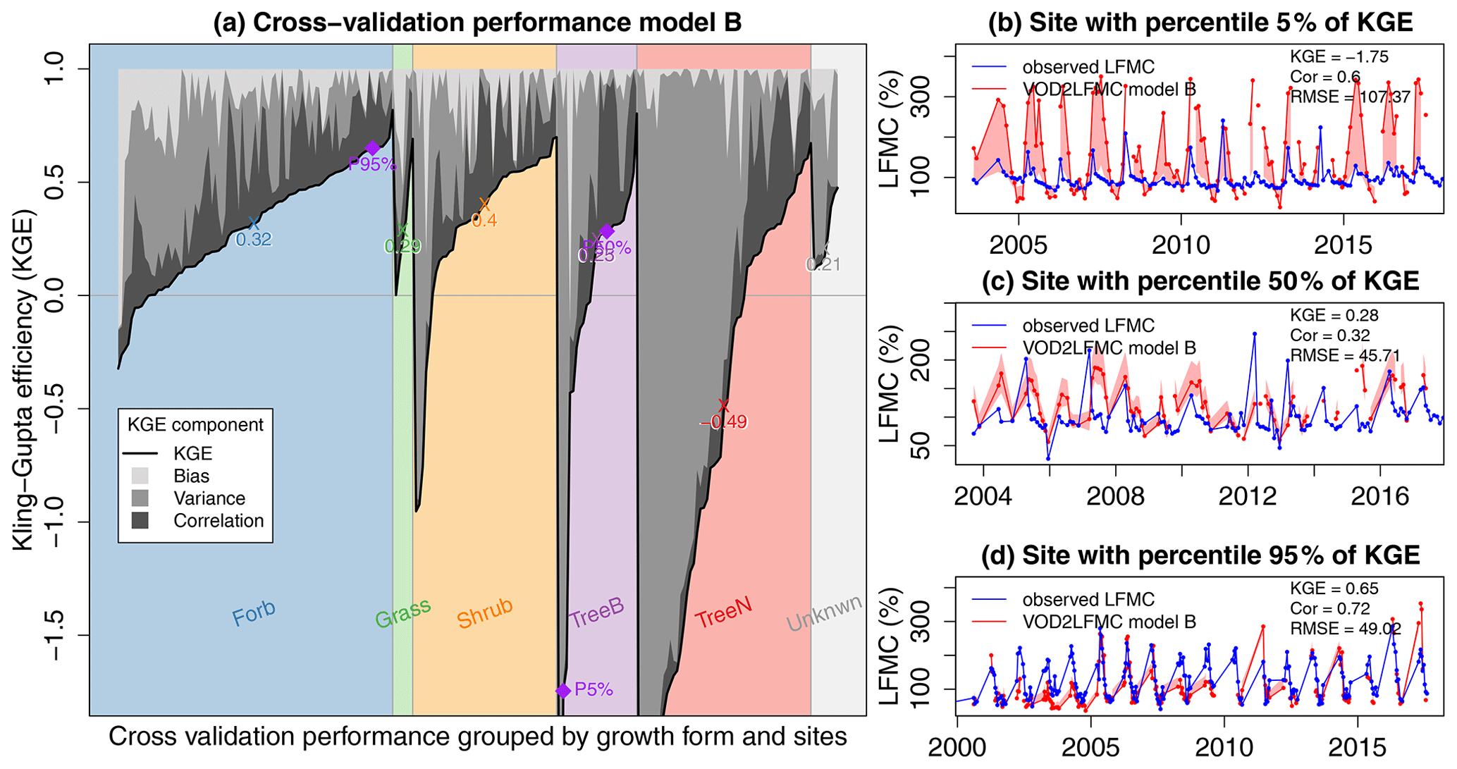
Figure 7 Performance of Model B using Ku-VOD in spatial cross-validation at each site grouped by the sampled vegetation growth form of LFMC measurements. (a) Kling–Gupta efficiency with its components caused by bias, variance, and correlation. Purple dots represent the 5th, 50th, and 95th percentiles of the KGE across all sites. The time series of the sites corresponding to those percentiles are shown in panels (b, 5 % = site with low performance, broad-leaved tree site), (c, 50 % = site with medium performance, broad-leaved tree site), and (d, 95 % = site with good performance, forb site).

3.3.2 Spatial applicability of model structures

The ranking in performance of the four models in spatial cross-validation resembles the ranking of the performance in site-level calibrations. On the one hand, the large variability in performance at site-level calibration and the strong decrease in performance in spatial cross-validation for Model C demonstrates that this model cannot be successfully applied and transferred to estimate LFMC globally. On the other hand, the results demonstrate that Model B can be successfully used to estimate the spatial–temporal dynamics of LFMC, whereby the parameters of model B can be estimated from observed tree cover using random forest. Medium to high performance of the estimated LFMC can be expected for herbaceous vegetation, shrublands, and for most broad-leaved trees. On average, a low performance and underestimation of the observed variance can be expected for needle-leaved trees, but this is not the case for all sites with needle-leaved trees.

The application of Model B in estimating LFMC results in performances (i.e. median RMSE = 48.8 % in global spatial cross-validation) that are comparable with other studies that estimated LFMC based on optical satellite observations. For example, estimated LFMC reached errors of 40 % (Yebra et al., 2018), 45 % (Caccamo et al., 2011) and 44 % (Nolan et al., 2016) across validation sites in Australia (Yebra et al., 2018) and approx. 34% in a global study with MODIS data (Quan et al., 2021). Rao et al. (2020) used Landsat-8 and Sentinel-1 Radar backscatter to estimate LFMC for the western US using a neural network model and obtained RMSE of 25 % across vegetation types. They obtained the lowest errors for mixed and needle-leaved forests (RMSE = 20 % and 22 %) and the highest errors for grasslands (RMSE = 31 %). While our results are similar for site-level calibrations of model B (i.e. RMSE = 15 % for needle-leaved trees and 39 % for grasslands), we found much lower performance for needle-leaved trees in spatial cross-validation.

The lower performance of Model B for needle-leaved trees in spatial cross-validation than at site-level calibration indicates that the calibrated parameters from each site cannot be well estimated in space. We assume that this is caused by the spatial representativeness of the used LFMC sites with needle-leaved trees. All of the used sites with needle-leaved trees are located in the western US and most of the sites are located in regions with low tree cover. Only a few sites are located in regions with higher tree cover and those sites are distributed across different spatial clusters for cross-validation. Hence, needle-leaved trees are included in 11 out of 20 spatial clusters and six of the spatial clusters include less than three sites with needle-leaved trees. This implies that in such cases, the training of model parameters is mostly based on sites without needle-leaved trees and from other regions, which will result in a low performance for needle-leaved forests. Those results suggest that still all vegetation types should be considered in spatial cross-validation in order to obtain realistic results for under-represented vegetation types.

Overall, our estimates of LFMC from coarse-resolution VOD and LAI data reach medium to high performances for most vegetation types that are comparable with other studies that use more data with higher spatial resolution or data from optical satellite systems for which the physical relations between LFMC and surface reflectance are established for several years (Yebra et al., 2013).

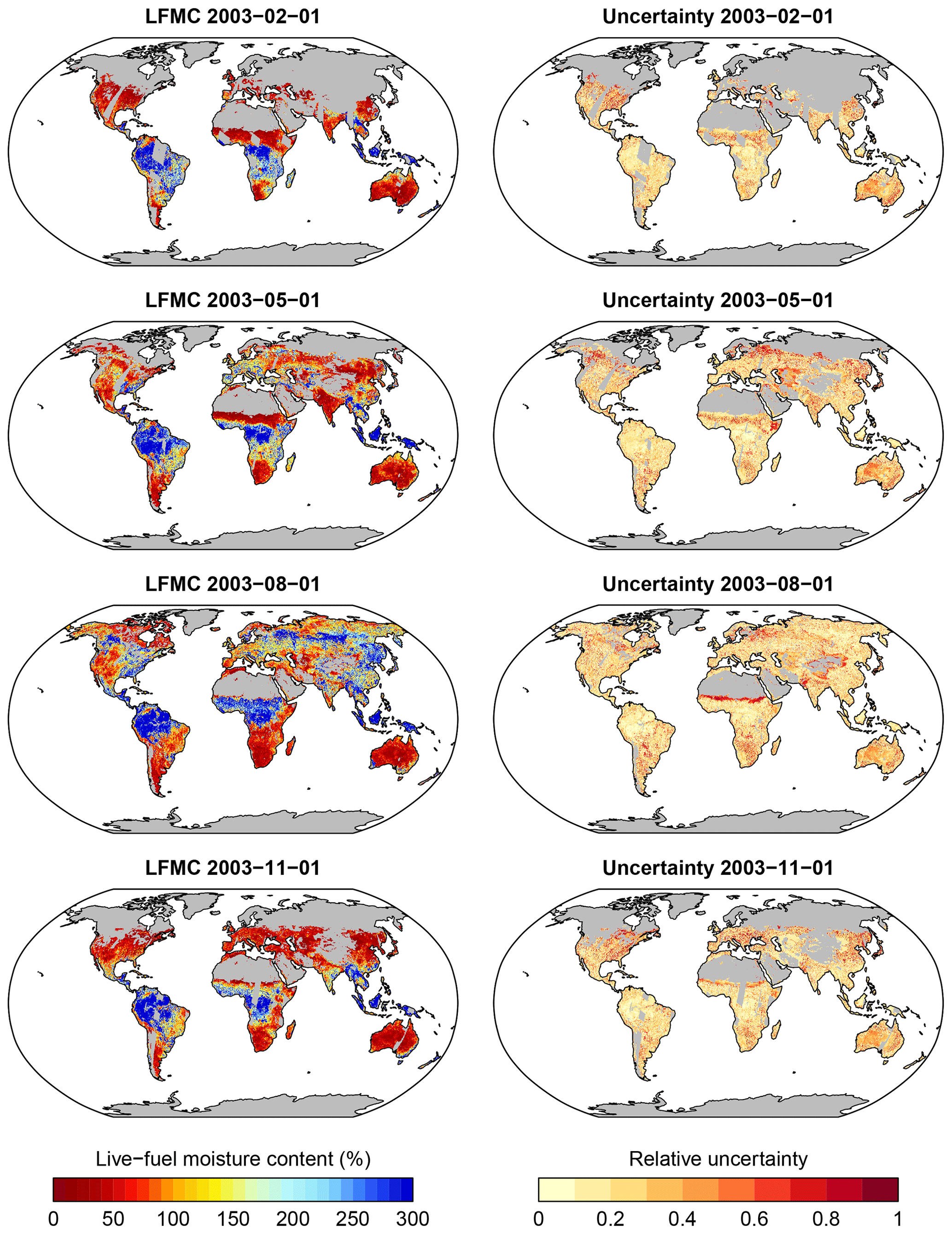
Figure 8 Example of global patterns of LFMC and associated uncertainties as estimated with Model B for 4 selected days in 2003, representing typical days during the northern seasons and the wet and dry seasons in Africa. Grey areas (missing data) is because of missing vegetation cover or gaps in the LAI or VOD data.

3.4 Global LFMC estimates

3.4.1 Global spatial–temporal patterns

Finally, we applied model B and the associated RF-based parameters to global data of Ku-VOD, LAI, and tree cover to estimate LFMC globally at 0.25×0.25^∘ spatial resolution and at daily sampling for the period February 2000 to July 2017 (overlapping period of Ku-VOD and MODIS LAI). As an example, we show global estimates for four dates in the year 2003 (Fig. 8). The four dates cover the different seasons in northern ecosystems as well as wet and dry seasons in tropical Africa. The four maps show generally high LFMC in wet tropical regions (Amazon and Congo basins, SE Asia), medium LFMC in many sub-tropical and temperate regions, and low LFMC in Savannah and desert regions. Seasonal changes in LFMC generally follow wet and dry seasons in semi-arid regions and the course of the phenological development as commonly seen in other vegetation properties (i.e. LAI or productivity). For example, the Sahel in northern Africa shows high LFMC in August (wet season) and low LFMC in February (dry season). Similar seasonal changes between wet and dry seasons can be seen in South America, the southern United States, the Mediterranean, India, eastern Asia, and Australia. The seasonal changes in LFMC are also visible in the Hovmöller diagram (Hovmöller, 1949) shown in Fig. 9. Thereby, equatorial regions show continuously high LFMC with a very weak seasonality. Northern subtropical regions between 5 and 18^∘ N show prolonged dry seasons with low LFMC towards northern latitudes. Northern mid- and high latitudes (>30^∘ N) show higher LFMC during the summer months than during spring and autumn.

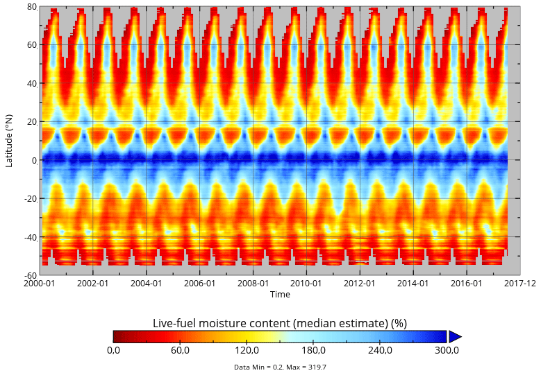
Figure 9 Hovmöller diagram of monthly LFMC as estimated from Model B using daily Ku-VOD and monthly LAI.

The large similarity of the global seasonal changes in LFMC with similar changes found in other vegetation properties such as LAI or gross primary productivity might seem astonishing at first view because LFMC represents a relative property of moisture content and not an absolute property of vegetation cover or biomass (like LAI). However, seasonal changes in leaf cover are highly correlated with LFMC, especially in short vegetation regions. For example, MODIS LAI has an across-site median temporal correlation with measurements of the Globe-LFMC dataset between r=0.30 and r=0.50 for regions with short vegetation cover > 80 % (Fig. A5). Hence the Globe-LFMC site-level data show indeed a strong coupling between LFMC and LAI, which is then also reflected in our global estimates of LFMC. This suggests a close coupling of LFMC increases with leaf development and of LFMC decreases with leaf cavitation and shedding.

Areas without estimates of LFMC (grey areas in Figs. 8 and 9) occur because of several reasons. (1) Missing data in deserts and ice-covered regions are because the model was not applied to grid cells with less than 5 % vegetation cover. (2) Missing data in northern latitudes in winter months are either because of months without LAI observations because of low solar zenith angles, snow or cloud cover, or because Ku-VOD observations were not available over frozen soils. (3) Other days with missing observations in some regions are because of missing coverage of passive microwave sensors or were masked in the VODCA dataset because of RFI.

We also compared the estimated LFMC from Model B with MODIS-LFMC for Australia and Europe to assess the similarity of both datasets. However, as the VOD-based LFMC uses monthly LAI from MODIS as input, which is derived from the same spectral bands like MODIS-LFMC, both LFMC datasets are not independent of each other and a high correlation can be expected. Indeed both the VOD-based LFMC and MODIS-LFMC are highly correlated (Fig. A3). The spatial patterns of correlation between the VOD-based LFMC and MODIS-LFMC show similar regions where Ku-VOD already had high and low correlations with MODIS-LFMC, respectively (Fig. 1). The correlation between VOD-based LFMC and MODIS-LFMC is higher than between Ku-VOD and MODIS-LFMC in many regions, which is likely due to the additional use of MODIS-LAI in Model B. The low correlation in parts of northern Europe and the Alps was already present in the correlation between MODIS-LFMC and Ku-VOD. The low correlation between VOD-based LFMC and MODIS-LFMC in northern Europe can be additionally caused by the low performance of the estimates in needle-leaved forests, which are widespread in those regions. However, the very high correlation between VOD-based LFMC and MODIS-LFMC demonstrates in many regions and in most fire-prone regions a good comparability of the two datasets.

3.4.2 Uncertainties and observational support

The uncertainty estimates of the global LFMC estimates are on average low (global mean relative uncertainty = 0.28) and do not show distinct spatial patterns (Fig. 8, right column). Larger relative uncertainties tend to occur at low LFMC, i.e. at seasonally dry conditions or in transitions areas to deserts (e.g. the Sahel, border of Sahara, Central Asia, parts of Australia) and in the boreal forest regions in Russia and Canada. The higher uncertainty over boreal forests corresponds to the lower correlations between LFMC and Ku-VOD and between estimated and observed LFMC after site-level calibration, and to the lower performance in spatial cross-validation for sites with needle-leaved trees.

The analysis of the estimated global patterns of LFMC needs to be compared with the number of observations that support the global estimates. The majority of pairs of Ku-VOD and Globe-LFMC observations come from the western US and from sites in the Mediterranean, western Africa, and southern Australia (Fig. A4a). The available Globe-LFMC observations cover mean annual temperatures between −0.3 and 27 ^∘C and annual total precipitation between 202 and 1465 mm (Fig. A4c). This indicates that boreal and polar regions and very wet tropical regions are generally not supported by Globe-LFMC observations. Likewise, the observations cover tree coverages between 0 % and 79 %, but no observations are available at high tree cover with high mean annual temperature > 20 ^∘C (i.e. in tropical forests) (Fig. A4d).

We additionally estimated the number of supporting observations in space as a function of mean annual temperature, tree cover, maximum Ku-VOD, and maximum LAI (Fig. A4b). Therefore, a random forest regression was fitted to the number of observations per site in the Globe-LFMC database and by using mean annual temperature, tree cover, mean annual maximum Ku-VOD, and mean annual maximum LAI as predictors. The fitted random forest model was then applied to each 0.25×0.25^∘ grid cell to provide an estimate of how many observations actually support an LFMC estimate in a grid cell. We found that the global LFMC estimates are not supported by any site-level LFMC observations with similar conditions in most of the tropical forests and in the boreal forests in Eurasia. However, most temperate and semi-arid regions are supported by Globe-LFMC observations. In addition, large areas of high northern latitudes (including most of the polar Tundra regions) are supported by Globe-LFMC observations because they have similar conditions of low tree cover, LAI, and Ku-VOD, like some sites in mountainous areas in the western US or the existing sites in Alaska. However, as many sites in mountainous regions have low correlations between VOD and LFMC (Fig. 1), the plausibility of LFMC estimates in northern latitudes is questionable. However, the global estimates of LFMC have strong observational support by site-level observations in many fire-prone regions such as in western Canada, the western US and Mexico, in southern South America, in the Mediterranean, central Asia, parts of China, southern and eastern Africa, and southern and eastern Australia. This provides confidence that the LFMC estimates can be used as a predictor for fire dynamics in most fire-prone ecosystems.

3.5 Applicability of the LFMC estimates and future directions

The aim of this study was to investigate the VOD–LFMC relationship and to develop and test model approaches to estimate LFMC globally. We also generated a daily LFMC dataset for past conditions, whereby the daily information originates from the Ku-VOD data. Although the presented LFMC dataset has a much coarser spatial resolution than MODIS-LFMC datasets (Yebra et al., 2018; Quan et al., 2021; Zhu et al., 2021), the advantages are the daily coverage, because VOD is cloud- and illumination-independent, and the long timespan of VOD data (e.g. Ku-VOD starting in 1987), which potentially allow to produce long-term estimates of LFMC in future studies. Hence, the described methodology to estimate LFMC from VOD can complement LFMC retrievals from optical sensors by providing a higher temporal frequency and potentially a longer temporal coverage.

We envision several applications of the global Ku-VOD-based estimates of leaf moisture content (expressed as LFMC), but also want to raise attention to the limitations of the dataset in other applications. The VOD-based LFMC estimates are suitable to investigate large-scale patterns of vegetation responses to drought, to assess fire danger and to estimate fire emissions, or to benchmark global ecohydrological and fire-enabled vegetation models.

3.5.1 Application of the LFMC estimates as drought indicator

Several remotely sensed vegetation properties such as spectral vegetation indices, LAI, sun-induced fluorescence, or derived variables of plant productivity are frequently used to monitor drought effects on vegetation (e.g. Jiao et al., 2021; Crocetti et al., 2020) or to investigate the effects of water availability on vegetation growth. The VOD-based LFMC estimates can complement such analyses by providing information on large-scale changes in leaf moisture content.

As a case study, we compared the VOD-based LFMC with drought conditions in North America and specifically in California by using the 12-monthly Standardized Precipitation Index (SPI-12) and the US Drought Severity and Coverage Index (DSCI) (Fig. 10). August 2014 was one of the most severe drought months in the western US. The VOD-based LFMC estimates show widespread patterns of very low LFMC over the western US during this month (Fig. 10a). This corresponds to a lack in precipitation as indicated by the negative SPI-12 (Fig. 10b). Also, large regions in northern Canada show precipitation deficit with low SPI-12 in northern Canada, which also corresponds to patterns of low LFMC.

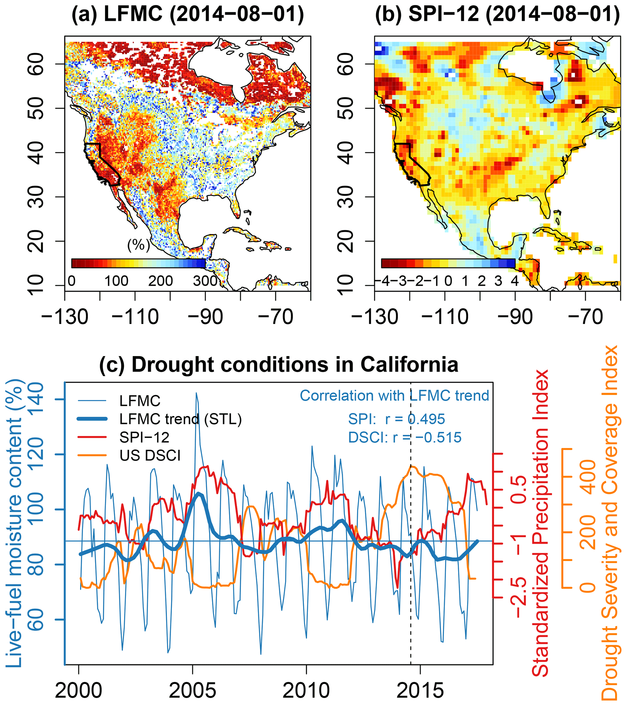
Figure 10 Comparison of LFMC as estimated from model B with drought conditions in North America and California. (a) Map of mean monthly LFMC for August 2014, a month with severe drought in the western United States. The state of California is highlighted in the map. (b) Map of the Standardized Precipitation Index for 12-monthly accumulation periods (SPI-12) for August 2014. SPI-12 data are taken from Global Drought Observatory – JRC European Commission (2022). (c) Comparison of LFMC, SPI-12, and the US Drought Severity and Coverage Index (DSCI) for California. A severe drought started in California (and in the western US) in 2013 and lasted until end 2016, as shown by negative SPI-12 values, very high DSCI values, and low LFMC. The dashed vertical line corresponds to August 2014, which is shown as map in panels (a) and (b).

To investigate multi-year drought events, we also compared LFMC, SPI-12, and DSCI time series averaged for the state of California (Fig. 10c). Both SPI-12 and the DSCI show the multi-year drought between 2013 and 2016. The LFMC time series is dominated by the strong seasonal signal. Therefore, we decomposed the LFMC time series for California into a seasonal, trend, and remainder component using the seasonal decomposition of time series by Loess (STL) method (Cleveland et al., 1990). The LFMC trend shows a long period of low values between 2013 and 2016, which corresponds to the drought period. Likewise, the wet period between 2005 and 2007 with higher precipitation (i.e. high SPI-12) and no drought conditions (i.e. DSCI close to 0) corresponds to high LFMC values. The LFMC trend component is medium correlated with SPI-12 (r=0.495) and DSCI ($r=-\mathrm{0.515}$), and hence reflects well the inter-annual variability of drought and wet conditions. This continental/regional case study demonstrates the potential to investigate effects of multi-year drought conditions and climate variability on vegetation moisture with the VOD-based LFMC estimates.

3.5.2 Applications for large-scale fire science

Generally, the main application of LFMC data is the assessment of fire risks (Chuvieco et al., 2010). The high temporal frequency and long period of the VOD-based LFMC dataset allow investigating short-term to long-term changes in fuel moisture and hence fire risk at a large scale. Previously, VOD datasets have been used as proxies for fuel conditions in global empirical models of burned area (Forkel et al., 2017; Kuhn-Régnier et al., 2021) and helped to explain how trends in climate conditions and vegetation affect large-scale trends in burned area (Forkel et al., 2019). However, the interpretation of VOD effects on the prediction of burned area was hampered in those studies by the unclear role of VOD as a proxy for fuel loads (biomass) or fuel moisture content. The VOD-based LFMC estimates overcome this problem by translating VOD into LFMC. Besides in empirical models for large-scale burned area, the VOD-based LFMC estimates can be used to investigate changes in fire radiative energy or fire emissions, which both depend on fuel moisture content. Further investigations could assess the predictive performance of the VOD-based LFMC data within large-scale empirical modelling studies to predict burned area or other properties of fire dynamics.

However, the coarse spatial resolution of the VOD-based LFMC data ($\mathrm{0.25}{}^{\circ }\times \mathrm{0.25}{}^{\circ }$) prevents applications in regional and local fire risk assessment. At a small scale, differences in vegetation structure and topography are the main controls on fire ignitions and propagation (Chuvieco et al., 2010), which are not accounted for in the VOD-based LFMC dataset. Hence, an application of the VOD-based LFMC estimates for regional fire risk assessment should be tested with caution, especially in heterogeneous landscapes or mountainous regions. However, our cross-validation results suggest that the LFMC estimates can be applied in large homogenous landscapes with short vegetation types.

Furthermore, the VOD-based LFMC estimates can contribute to the evaluation and improvement of moisture simulations in global ecohydrological and fire-enabled vegetation models such as from the fire-model inter-comparison project (FireMIP) (Rabin et al., 2017). FireMIP models simulate live and dead fuel moisture either based on fire danger indices (e.g. the Nesterov index, Thonicke et al., 2010) or based on empirical functions with soil moisture or relative humidity (Rabin et al., 2017). FireMIP models have been intensively evaluated for simulations of burned area, fire emissions, LAI, plant productivity, and biomass (Hantson et al., 2020), and the simulated fuel moisture has a strong effect on simulations of burned area and fire emissions (Li et al., 2019). However, fuel moisture has not yet been evaluated in those models. Hence, we propose that the VOD-based LFMC estimates or other global products (Quan et al., 2021) can be used in benchmarking activities of global fire-enabled vegetation models.

3.5.3 Future developments

Finally, we propose several further developments of the VOD-based LFMC datasets:

• The calibration and evaluation of the applied models used only 163 sites out of 1384 sites in the Globe-LFMC database according to the selection criteria described in Sect. 2.5. This is mainly caused by the joint availability of pairs of LFMC/VOD observations. Additionally, our selection criteria also prevented us from using the measurements from all 229 sites in China, where each site has only one measurement. Future developments can apply different approaches to make use of more observations in model training. While sites with single measurements cannot be used to calibrate models at site level, they could be still used in training the spatial random forest model to estimate model parameters. At other sites, a filling of short temporal gaps in VOD time series could increase the availability of LFMC/VOD pairs and would increase the number of sites that can be used for model calibration.

• An estimation of LFMC for different vegetation types within a VOD grid cell can be explored as the site-level model calibration was performed for different vegetation growth forms reported in the Globe-LFMC database.

• LAI data at their original spatial resolution within the VOD-based models could be used to provide LFMC estimates at higher spatial resolution.

• One advantage of our methodology is the long timespan of VOD data (e.g. Ku-VOD starting in 1987), which potentially allows to produce long-term estimates of LFMC in future studies. Hence, the temporal coverage of the LFMC estimates can be extended back to 1987 by using longer LAI time series than provided by MODIS. Such an extension would also allow the use of older LFMC field data in model calibration. Such long time series of LFMC can facilitate climatological studies on the variability and LFMC and the potential effects on fire.

• The prediction of fire risks requires the availability of satellite products shortly after the observation. Our methodology could be applied to estimate LFMC in near-real time, however, this requires the availability of near-real time VOD products.

4 Conclusions

This study assessed the relationship between short-wavelength VOD from passive microwave satellite observations and leaf moisture content (expressed as LFMC) globally, and successfully developed and applied a method to estimate LFMC from VOD globally at $\mathrm{0.25}{}^{\circ }\times \mathrm{0.25}{}^{\circ }$ spatial resolution, at daily time steps, and for the period from February 2000 to July 2017. We achieved our three objectives as follows:

1. We investigated the relationship between VOD and LFMC. VOD and LFMC are in the majority of sites or grid cells positively correlated, whereby Ku-band VOD has slightly higher correlations than X- or C-VOD. The correlation between VOD and LFMC is on average higher for short vegetation types such as forbs, grasses, and shrubs than for trees, but also several forest sites show high correlations. Broad-leaved forests show higher correlations than needle-leaved forest. These results confirm earlier studies about the VOD–LFMC relation and demonstrate additionally that coarse-scale VOD is sensitive to LFMC at forest sites if the land cover distribution locally is similar to the coarse grid cell.

2. We tested different model structures to estimate LFMC from VOD. A logistic regression model that uses daily Ku-VOD and monthly LAI as predictors for LFMC outperformed alternative model structures in site-level calibration and spatial cross-validation. The comparison of model structures demonstrates that LAI is needed in addition to VOD as a proxy for either canopy biomass or vegetation water content to reach acceptable model performances.

3. We applied spatial cross-validation to assess the transferability of model structures in space and applied the best-performing model to estimate LFMC globally. The obtained model performances are comparable with results from previous studies that estimated LFMC based on visible/near-infrared satellite observations. Medium to high performance of the VOD-based LFMC estimates can be expected for herbaceous vegetation, shrublands, and for most broad-leaved trees in many fire-prone regions, such as in western Canada, the western US and Mexico, in southern South America, in the Mediterranean, central Asia, parts of China, southern and eastern Africa, and southern and eastern Australia. Large variability in performance and high uncertainties can be expected in needle-leaved forests, whereby especially estimates in boreal forest have low observational support.

We propose to use VOD-based estimates of LFMC to investigate effects of drought and climate variability on vegetation leaf moisture at large scale, for large-scale assessments and empirical modelling of fire dynamics, or to benchmark global fire-enabled vegetation models.

Appendix A

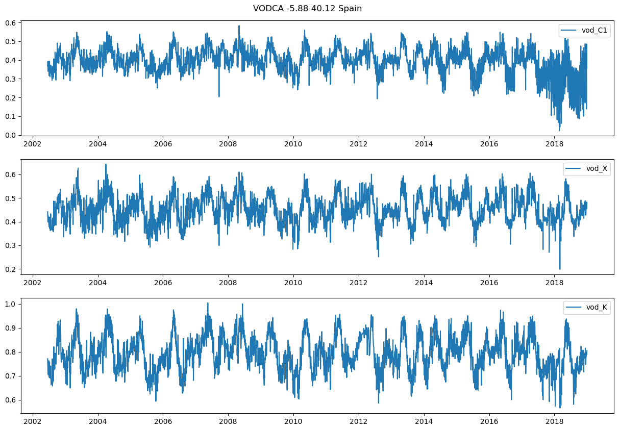
Figure A1 Example time series of C-, X-, and Ku-VOD over a grid cell in Spain (5.88^∘ W, 40.12^∘ N), where the C-VOD time series shows a high level of noise likely caused by RFI in the later years.

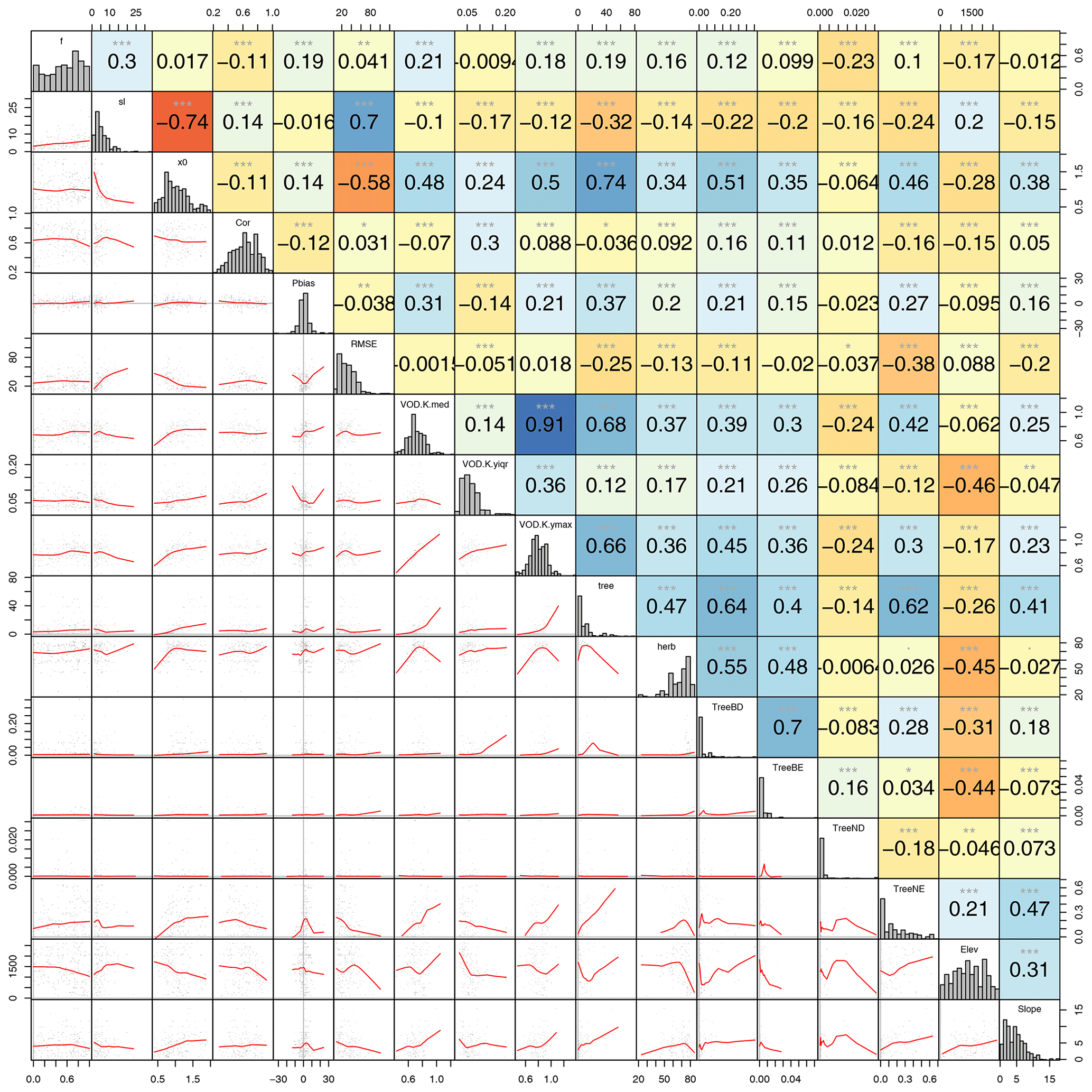
Figure A2 Across-site correlations between the site-optimized parameters f, sl, and x₀ of Model B with model performance measures and land cover properties of the corresponding 0.25^∘ grid cells. Numbers and blue to red colours in the upper triangle display Spearman correlation coefficients. Red lines in the lower triangle are Loess fits between x and y values. Grey bars along the diagonal are histograms of each variable. Correlation (Cor), percent bias (Pbias), and RMSE of predicted and observed LFMC; temporal median of Ku-VOD (VOD.K.med); multi-year mean of the annual interquartile range of Ku-VOD (VOD.K.yiqr); multi-year mean of annual maximum Ku-VOD (VOD.K.ymax); tree and short vegetation cover from Song et al. (2018); tree cover of broad-leaved deciduous (TreeBD), broad-leaved evergreen (TreeBE), needle-leaved deciduous (TreeND), and needle-leaved evergreen (TreeNE) trees (ESA CCI Land cover V2.0.7 dataset); elevation (Elev) and slope from the CGIAR CSI SRTM digital elevation model.

Figure A3 Pearson correlation between the VOD-based LFMC from Model B and MODIS-LFMC for Australia and Europe for the time period February 2000 to July 2017.

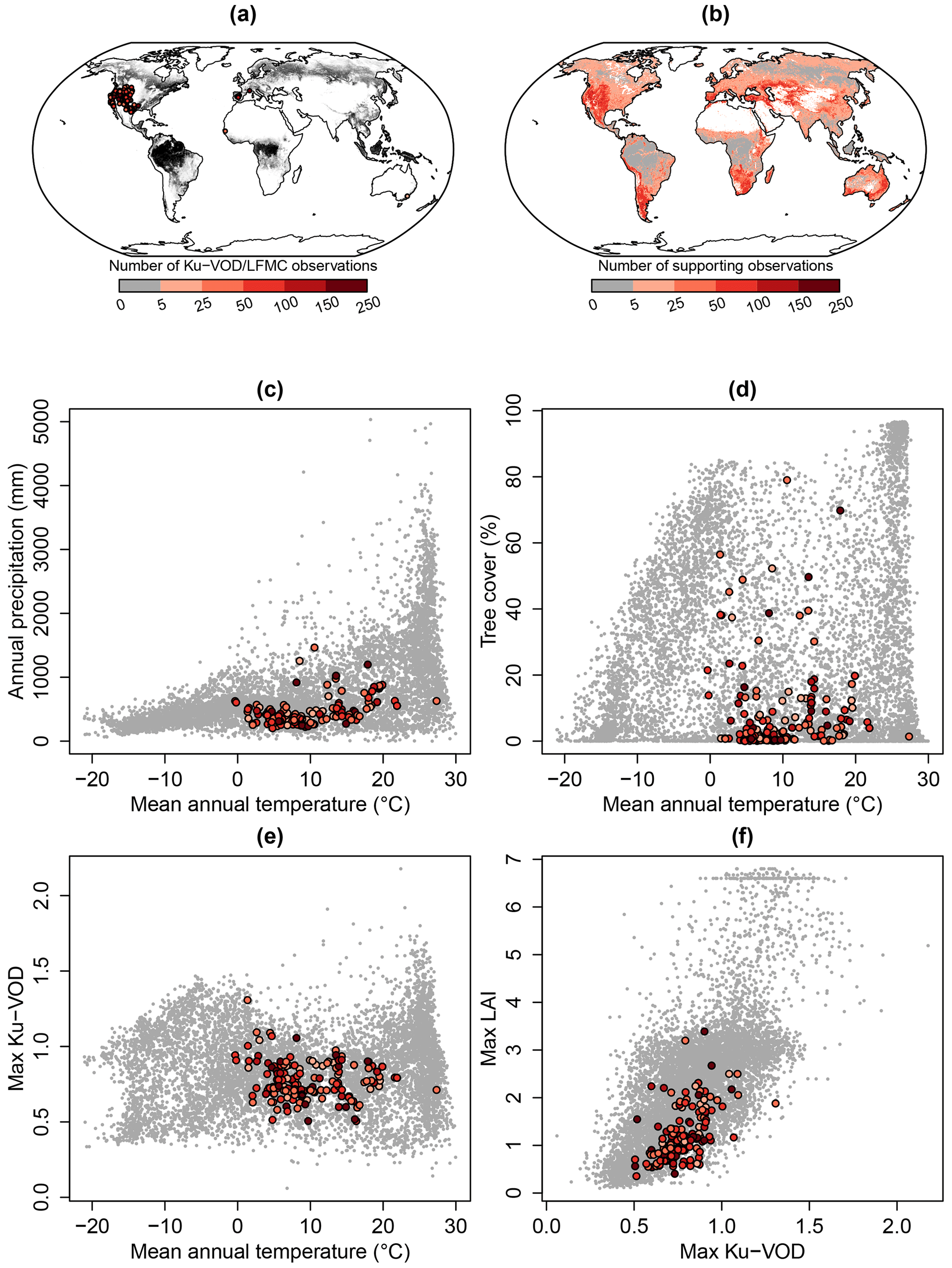
Figure A4 Distribution of the number of joint observations of Ku-VOD and Globe-LFMC measurements. (a) Distribution of Globe-LFMC sites overlaid over the percentage tree cover. (b) Spatial estimate of the number of supporting observations that indicates how many pairs of Ku-VOD/Globe-LFMC observations are available with similar mean annual temperature and vegetation conditions (i.e. LAI, tree cover, Ku-VOD). To create this map, a random forest regression was fitted to the number of observations shown in (a) and by using mean annual temperature, tree cover, mean annual maximum Ku-VOD, and mean annual maximum LAI as predictors. The fitted random forest model was then applied to each 0.25^∘ grid cell to provide an estimate of how many observations are actually supporting an LFMC estimate in a grid cell. (c, d) Number of observation within the global feature space of mean annual temperature and annual total precipitation (c) and mean annual temperature and tree cover (d).

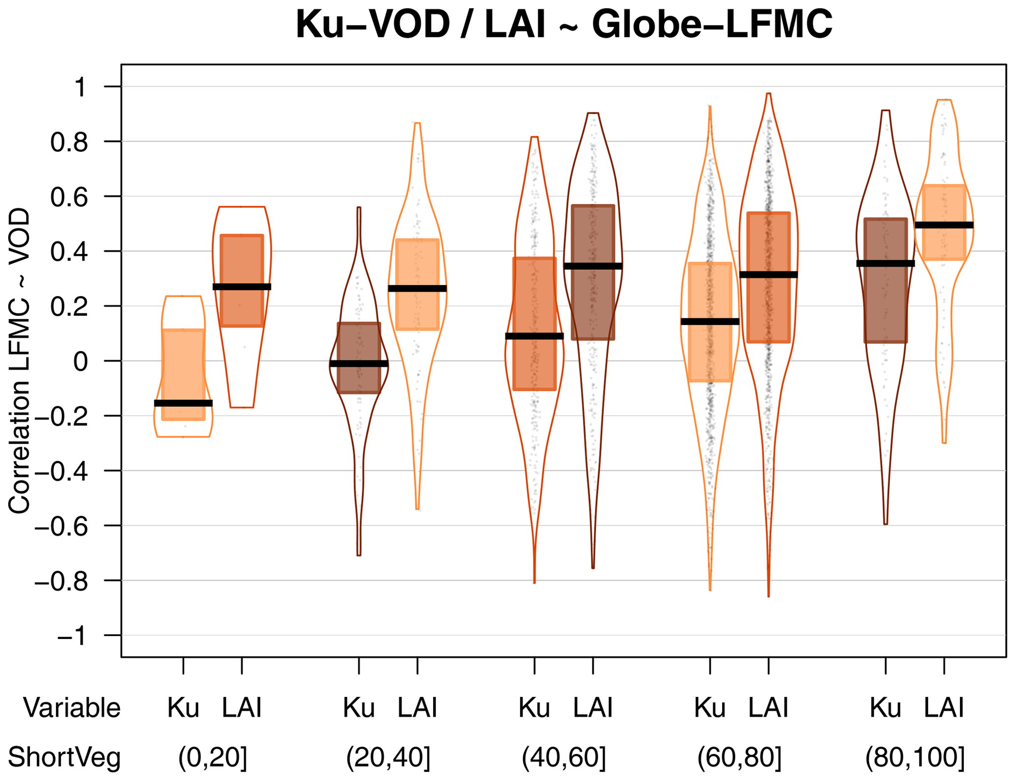
Figure A5 Statistical distributions of the temporal correlation between Ku-VOD or LAI and measurements from the Globe-LFMC database stratified by the percentage cover of short vegetation.