Remote quantification of the trophic status of Chinese lakes

Assessing eutrophication in lakes is of key importance, as this parameter constitutes a major aquatic ecosystem integrity indicator. The trophic state index (TSI), which is widely used to quantify eutrophication, is a universal paradigm in the scientific literature. In this study, a methodological framework is proposed for quantifying and mapping TSI using the Sentinel Multispectral Imager sensor and fieldwork samples. The first step of the methodology involves the implementation of stepwise multiple regression analysis of the available TSI dataset to find some band ratios, such as $\mathrm{blue}/\mathrm{red}$, $\mathrm{green}/\mathrm{red}$ and $\mathrm{red}/\mathrm{red}$, which are sensitive to lake TSI. Trained with in situ measured TSI and match-up Sentinel images, we established the XGBoost of machine learning approaches to estimate TSI, with good agreement (R²= 0.87, slope = 0.85) and fewer errors (MAE = 3.15 and RMSE = 4.11). Additionally, we discussed the transferability and applications of XGBoost in three lake classifications: water quality, absorption contribution and reflectance spectra types. We selected XGBoost to map TSI in 2019–2020 with good-quality Sentinel-2 Level-1C images embedded in the ESA to examine the spatiotemporal variations of the lake trophic state. In a large-scale observation, 10 m TSI products from 555 lakes in China facing eutrophication and unbalanced spatial patterns associated with lake basin characteristics, climate and anthropogenic activities were investigated. The methodological framework proposed herein could serve as a useful resource for continuous, long-term and large-scale monitoring of lake aquatic ecosystems, supporting sustainable water resource management.

1 Introduction

Lakes, as valid sentinels of global or regional responses, are sensitive to anthropogenic activities and climate change (Mortsch and Quinn, 1996; Quayle et al., 2002; Tranvik et al., 2009). The commonly used paradigm for studying eco-environmental monitoring and controlling of lakes is the status of eutrophication (Carlson, 1977). It is a combination of light, heat, hydrodynamics and nutrients, such as nitrogen and phosphorus, which occurs through a series of biological, chemical and physical processes of lakes (Guo et al., 2020). As a result of eutrophication, nutrient loading and productivity grow sharply, and even hypoxia and frequent outbreaks of harmful algal blooms are likely to produce toxins (Paerl, 2008; Paerl et al., 2011). These processes can cause serious degradation of water quality and are detrimental to the ecosystem service functionality of lakes and the reliable supply of drinking water (OECD, 1982). Once the eutrophication phenomenon becomes intense, ecological imbalances generally follow (Smith et al., 2006). Hence, knowledge of eutrophication processes can provide us with an understanding of the structure and function of lake ecosystems that give rise to environmental changes. We can then predict future trends and develop appropriate mitigation strategies.

Several lakes experience eutrophication processes because of excessive nutrient enrichment (Lund, 1967; Smith et al., 1999; Wetzel, 2001). At the global scale, 63.1 % of lakes larger than 25 km², 54 % of Asian lakes (Wang et al., 2018) and 53 % of European lakes (ILEC et al., 1994) are eutrophic. Lake eutrophication has become a global water quality issue affecting most freshwater ecosystems (Matthews, 2014). Currently, many pollution control measures and management strategies have been implemented that are specific to individual lakes or to lakes in general. However, there is still insufficient information to address lake eutrophication related to environmental disturbances or changes. Realization of lake eutrophication has been a serious situation for some lakes; therefore, we provided some reasons to suggest the need for large-scale research. First, different environmental factors control the trophic status of lakes at local and multiple scales (e.g., Wiley, 1997). Specifically, biotic factors may dominate the eutrophic state of individual lakes, and we can understand the mechanism processes by lake-specific sampling. In contrast, abiotic factors and their linkages are pivotal factors that determine lake biogeochemistry at multiple scales (Sass et al., 2007). It is often necessary to study a number of lakes with different characteristics and catchments to understand the mechanisms of spatiotemporal patterns. Therefore, an upscaling study of trophic status is required to understand the evolution prospects of lakes in response to changes in global and regional environments. Second, multiyear environmental and climatic conditions require long-term field studies and observations to understand the temporal pattern in important trophic status processes. In addition, relatively large datasets are needed considering the spatial extent because environmental factors are integrated to determine the trophic status of lakes. It can promote data organization and enable us to address an emergency and establish scientific measures for water resource management (Cunha et al., 2013; Smith and Schindler, 2009). Thus, eutrophication should be rapidly assessed using easy-to-analyze indices and enforcement methods for large-scale and high-frequency applications.

Evaluating the trophic state of lakes has been an important topic for decades (Carlson, 1977; Smith and Schindler, 2009). The traditional method uses chlorophyll a, transparency, nutrients and other variables as water quality indicators by field in situ sampling and laboratory measurements (Rodhe, 1969). Subsequently, Carlson (1977) introduced a numerical trophic state index (TSI) that should have replaced descriptive values like “oligotrophic”, “mesotrophic” or “eutrophic”. The replacement has not occurred, but the TSI proposed by Carlson is a common method to determine the trophic state level of aquatic environments (Aizaki, 1981). The traditional method for calculating TSI is based on collected in situ data. The sampling itself and subsequent laboratory measurements are labor-intensive, expensive and often also logistically difficult to perform. This limits our capability to monitor hundreds or thousands of lakes for eutrophication, not speaking about the majority of the 117 million lakes on Earth (Verpoorter et al., 2014). Moreover, the TSIs calculated for one or a few discrete samples do not represent the spatial distribution of TSIs within (especially larger) lakes. This could limit the large-scale assessment of eutrophication and the understanding of biogeochemical cycles.

Satellite remote sensing is a useful tool for monitoring inland waters (Palmer et al., 2015). Ocean water-color sensors, such as the Medium Resolution Imaging Spectrometer (MERIS) or the Ocean and Land Colour Instrument (OLCI), have too low a spatial resolution (300 m) for the majority of lakes on Earth. Land remote-sensing sensors like the Landsat Operational Land Imager (OLI), the Sentinel-2 Multispectral Imager (MSI; 10–60 m) and the Satellite pour l'Observation de la Terre (SPOT) with a high spatial resolution (5–30 m) are not designed for water remote sensing (lack of critical spectral bands, signal-to-noise ratio (SNR) not being sufficient for water, etc.). Compared to the OLI and SPOT sensors, the MSI has a more adequate radiometric resolution (12 bits) and 13 spectral bands, including four visible and shortwave infrared (SWIR) channels (Drusch et al., 2012). Inland water TSI has been produced for large lakes using the MODIS sensor (Wang et al., 2018). However, this study is for more than 2000 large lakes (due to the spatial resolution of the sensor). The Copernicus Land Monitoring Service has started to produce TSI for lakes large enough to be mapped with 100 m pixel size using the Sentinel-2 MSI. However, this product is available only for Europe and some parts of Africa.

Instead of individual parameters, several studies (e.g., Morel and Prieur, 1977; Gurlin et al., 2011; Huang et al., 2014; Sass et al., 2007; Thiemann and Kaufmann, 2000; Yin et al., 2018) have also provided empirical relationships expressed as band combinations or baseline methods to acquire Chl a, transparency or nutrients related to potential TSI calculations in regional lakes. However, the accuracy of these empirical relationships for transferring knowledge from some representative lakes to large-scale lake groups is limited by large uncertainties (i.e., in areas with different water quality concentrations and atmospheric component influences, fewer lakes can be used with more heterogeneous influences and uniform algorithms) (Oliver et al., 2017). Considering the requirement of a uniform and universal relationship to quantify the trophic status of lakes, an alternative method using a high frequency and high spatial resolution of the sensor is a significant challenge. Recently, technological developments, such as machine learning algorithms, have allowed the usage of remotely sensed imagery to successfully investigate water quality parameters using artificial intelligence (Reichstein et al., 2019; Pahlevan et al., 2020; Cao et al., 2020). The potential application and development of machine learning for remote quantification of water quality are attributed to the following advantages: little prior knowledge is required, rich features can be captured, and robust relationships can be obtained. These processes avoid bias and uncertainty from the regional environmental background as well as complications due to atmospheric components of traditional remote-sensing-derived relationships over a large scale, i.e., for multiple lakes. Given the novel application of remote sensing and machine learning, this is a gap to fill for large-scale research of monitoring trophic states.

Environmental issues fueled by rapid economic growth in China have significantly increased in the last 3 decades. Lake eutrophication is a serious issue, with large variability in terms of trophic status and optical properties. However, most studies (Jin and Hu, 2003; Jin et al., 2005; Fragoso Jr. et al., 2011; Huang et al., 2014) have addressed eutrophication concerns in only a single lake or two lakes since the 1990s. It is acknowledged that a rapidly growing economy and anthropogenic activities (e.g., elevated nutrient loading and increasing air pollution) accelerate the aging process of lakes (Wu et al., 2011; Shi et al., 2020). Therefore, it is critical to objectively assess the trophic status and pay attention to protect the aquatic environment. We aim to provide a robust machine learning algorithm and remote-sensing flowchart from simultaneously retrieved TSI over a wide range of bio-optical compositions in different lakes. The objectives of our study were to (1) examine biogeochemical parameters and assess trophic status, (2) calibrate and validate the TSI model using different machining learning algorithms from MSI-imagery-derived remote-sensing reflectance spectra (R_rs) with different lake classifications, and (3) quantify and map the trophic status of 555 typical lakes in five Chinese limnetic regions.

2 Materials and methods

2.1 Study area and sampling process

China is located in the east of Asia with a land area of 9 600 000 km² and a population of over 1.4 billion. The terrain of China descends from west to east in three steps. Due to a vast territory span, this country has diverse climatic, geographical and geological conditions. There are 2693 natural lakes (with area > 1.0 km²) that are distributed in China (Ma et al., 2011). Protection and sustainable management of these lakes have been priorities, considering the degradation of water quality over several decades. In this study, a total of 45 lakes were visited and 431 samples were collected in early April 2016 to late October 2019 (Table S1 in the Supplement and Fig. 1), which was the highest productive season, as identified by Carlson's TSI model. These datasets were analyzed and published in Li et al. (2021) and Song et al. (2020). Our lake dataset was collected from various types of lakes across China, and efforts were made to examine lake trophic status from a wide range of water quality parameters, lake sizes (0.5 to 4, 256 km²), lake elevations (10 to 4, 525 m) and climatic zones (Song et al., 2019). In the field, some small-sized lakes were sampled in the middle, and a signal sample was used to represent the water qualities, while others were sampled at multiple locations evenly distributed over the lake. The water samples were collected approximately 0.5 m below the surface and then stored in 1 L amber HDPE (high-density polyethylene) bottles and kept in a portable refrigerator (4 ^∘C) before being transported to the laboratory. During the sampling process, the Secchi disk depth (SDD, m) was measured using a black-and-white Secchi disk. The pH and electrical conductivity (EC, µs cm⁻¹) were recorded using a portable multiparameter water quality analyzer (YSI 6600, 170 U.S.).

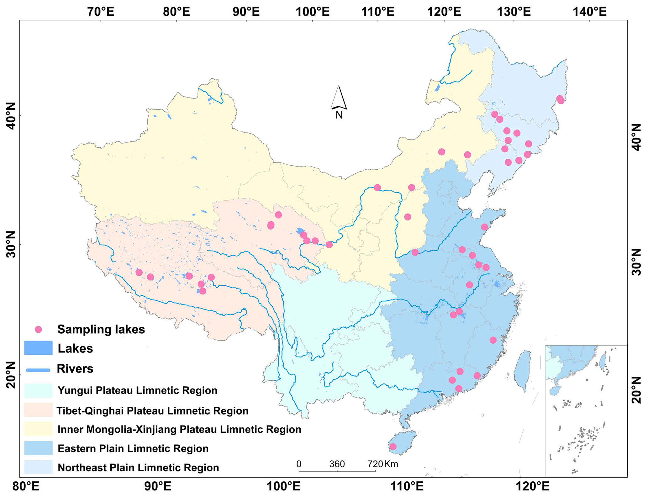
Figure 1 Locations of the lake sites.

2.2 Laboratory analysis

A transferred portion of each bulk water sample was immediately filtered with 0.45 µm pore size Whatman cellulose acetate membrane filters in the laboratory. It should be noted that some remote Tibet and Qinghai lake samples had to be filtered during fieldwork. Chlorophyll a (Chl a) was extracted from the filters using a 90 % buffered acetone solution at 4 ^∘C under 24 h dark conditions. According to the SCOR-UNESCO equations (Jeffrey and Humphrey, 1975), the concentration of Chl a (µg L⁻¹) was determined using a UV-2600PC spectrophotometer at 750, 663, 645 and 630 nm. Dissolved organic carbon (mg L⁻¹) concentrations were determined using a total organic carbon analyzer. Total nitrogen (TN) and total phosphorus (TP) concentrations (mg L⁻¹) were measured using a continuous-flow analyzer (SKALAR, San Plus System, the Netherlands) and a standard procedure (APHA/AWWA/WEF, 1998). In addition, total suspended matter (TSM, mg L⁻¹) concentrations were obtained gravimetrically using precombusted 0.7 µm pore size Whatman GF/F filters. All preprocesses (e.g., filtration and concentration quantification) of all water samples were undertaken within 2 d in the laboratory. The procedures are provided in detail in Li et al. (2021).

The bulk samples were again filtered through a 0.7 µm pore size glass-fiber membrane (Whatman, GF/F 1825-047) to retain particulate matter. The water from particulate matter measurements was then filtered through a 0.22 µm pore size polycarbonate membrane (Whatman, 110606) in order to measure the chromophoric dissolved organic matter (CDOM) absorption of each sample. According to the quantitative membrane filter technique (Cleveland and Weidemann, 1993), the light absorption of total particulate matter a_p(λ) can be separated into phytoplankton pigment absorption a_ph(λ), non-algal particles a_d(λ) and CDOM absorption a_CDOM(λ). The optical density (OD) of the particulate matter retained in the filters was measured using a UV-2600PC spectrophotometer at 380–800 nm, with a blank membrane as a reference at 380–800 nm. The filters were then bleached using a sodium hypochlorite solution to remove phytoplankton pigment and measured again using a spectrophotometer. Finally, the phytoplankton pigment absorption a_ph(λ) was calculated by subtracting a_d(λ) from the total particulate matter a_p(λ). The absorption coefficients of the optical active substances (OACs) were calculated according to Song et al. (2013a).

2.3 Trophic status assessment of lakes

Several studies have proposed different indices of the lake trophic state (Aizaki, 1981; Carlson, 1977). Carlson's trophic state index used five variables, such as Chl a, TP, TN, SDD and chemical oxygen demand (COD), to characterize the trophic state. However, there are no optical characteristics for TN, TP and COD to manifest in changes in remote-sensing reflectance, which may bring more uncertainties or errors. Thus, Chl a, TP and SDD were selected to assess the trophic status according to the modified Carlson TSI. The TSI can be calculated using individual TSI_M(Chl a), TSI_M(SDD) and TSI_M(TP) using the following equations:

$$\begin{array}{}\text{(1)}& {\displaystyle }{\mathrm{TSI}}_{\mathrm{M}}\left(\mathrm{Chl}a\right)=\mathrm{10}\times \left(\mathrm{2.46}+{\displaystyle \frac{\ln \mathrm{Chl}a}{\ln \mathrm{2.5}}}\right),\text{(2)}& {\displaystyle }{\mathrm{TSI}}_{\mathrm{M}}\left(\mathrm{SDD}\right)=\mathrm{10}\times \left(\mathrm{2.46}+{\displaystyle \frac{\mathrm{3.69}-\mathrm{1.52}\times \ln \mathrm{SDD}}{\ln \mathrm{2.5}}}\right),\text{(3)}& {\displaystyle }{\mathrm{TSI}}_{\mathrm{M}}\left(\mathrm{TP}\right)=\mathrm{10}\times \left(\mathrm{2.46}+{\displaystyle \frac{\mathrm{6.71}+\mathrm{1.15}\times \ln \left(\mathrm{TP}\right)}{\ln \mathrm{2.5}}}\right),\text{(4)}& {\displaystyle }\begin{array}{rl}\mathrm{TSI}=& \mathrm{0.54}\times {\mathrm{TSI}}_{\mathrm{M}}\left(\mathrm{Chl}a\right)+\mathrm{0.297}\times {\mathrm{TSI}}_{\mathrm{M}}\left(\mathrm{SDD}\right)\\ & +\mathrm{0.163}\times {\mathrm{TSI}}_{\mathrm{M}}\left(\mathrm{TP}\right),\end{array}\end{array}$$

where the TSI below 30 corresponds to oligotrophic waters, the TSI above 50 is eutrophic, and the TSI between 30 and 50 is mesotrophic (Carlson, 1977).

2.4 Multispectral imagery and atmospheric correction

Sentinel-2A and Sentinel-B MSI imagery was acquired from the Copernicus Open Access Hub of the European Space Agency. Altogether, 210 scenes of cloud-free Level-1C images covering the lakes were downloaded with a time window of ±7 d from in situ measurements. The Case 2 Regional Coast Color processor (C2RCC) was used to remove atmospheric effects. An average of 3 × 3 pixels centered at each in situ sampling station was used in the further analysis. All the processes were performed using the Sentinel Application Platform (SNAP) version 7.0.0. A flowchart of the process is shown in Fig. 2.

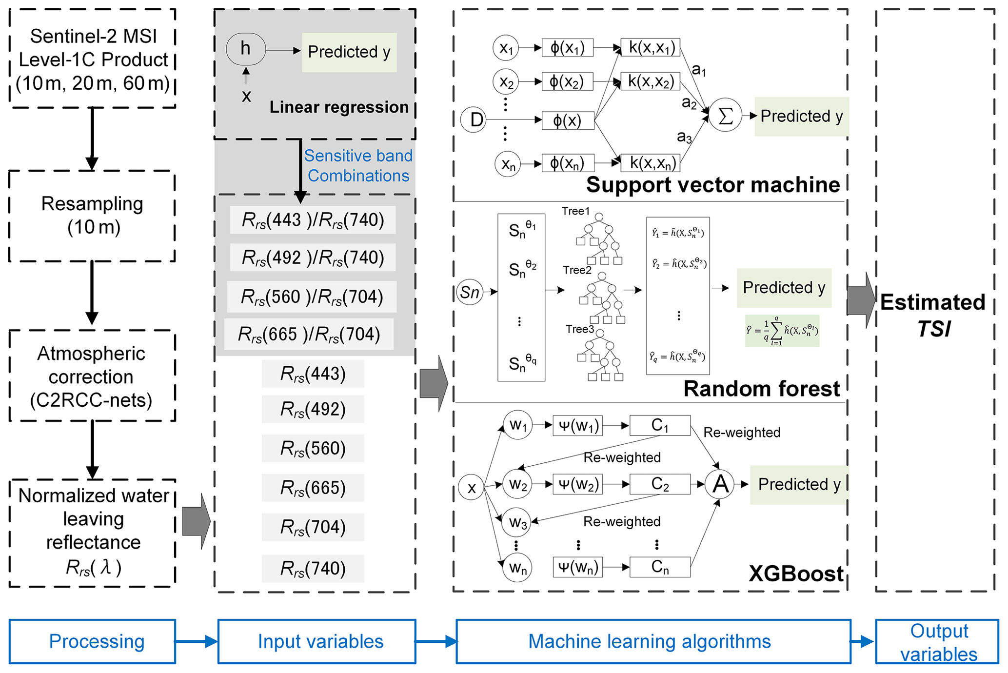
Figure 2 Workflow of the Sentinel-2 MSI data and machine learning algorithms for estimating TSI.

2.5 Machine learning algorithms

As a branch of artificial intelligence, the application of machine learning is growing in the field. Machine learning can automatically analyze huge chunks of data, develop optimal models, generalize algorithms and make predictions. These approaches have been applied in a variety of eco-environmental and remote-sensing fields (Mountrakis et al., 2011; Pahlevan et al., 2019). Hence, we employed four representative machine learning algorithms, i.e., linear regression (LR), support vector machine (SVM), XGBoost (XGB) and random forest (RF) (S1), to establish a TSI model. To strengthen the robustness, band combinations sensitive to TSI were determined by LR (Fig. 2) and were added to the procedure of machine learning algorithms as input variables. Subsequently, the output variable was the predicted TSI. The in situ measured samples were then randomly divided into a calibration dataset (70 %, 287 lake samples) and validation dataset (30 %, 144 lake samples) using MATLAB software. The TSI modeling procedure considering machine learning and multiple linear regression (MLR) was processed using the R software.

2.6 Classifications of lakes

In order to provide further feasibility for the application and availability of the TSI model, the in situ measured samples were classified in three ways (Fig. 3).

• a.

  They were based on water quality: salinity classification referred to the threshold value of electrical conductivity (named EC, EC = 1000 µS cm⁻¹) (Duarte et al., 2008), following which the lakes were divided into brackish lakes (N= 100 samples) and freshwater lakes (N= 331 samples). Dissolved organic carbon (DOC) in global lake water classification referred to the volume-weighted averaged DOC level of global lakes (3.88 mg L⁻¹) according to Toming et al. (2020), following which lakes were divided into high-DOC lake (N= 224 samples) and low-DOC lake (N= 207 samples).

• b.

  They were based on optical absorption contribution: optical absorption classification referred to Prieur and Sathyendranath (1981), where the total light absorption of water can be separated from phytoplankton pigment absorption, non-algal particles and CDOM absorption, respectively. The relative percentage of the absorption contribution of OACs can be divided into phytoplankton-type (Phy-type) lakes (N= 54 samples), non-algal-particle-type (NAP-type) lakes (N= 109 samples), CDOM-type lakes (N= 177 samples) and mix-type lakes (N= 91 samples).

• c.

  They were based on reflectance spectra: in order to discern the different optical characteristics of lakes, the derived MSI reflectance was clustered using the k-means clustering approach with a gap statistic (Neil et al., 2019). We identified 431 MSI reflectance R_rs(λ) spectra for three branches (Table S3), and the R_rs(λ) spectra are shown in Fig. 3.

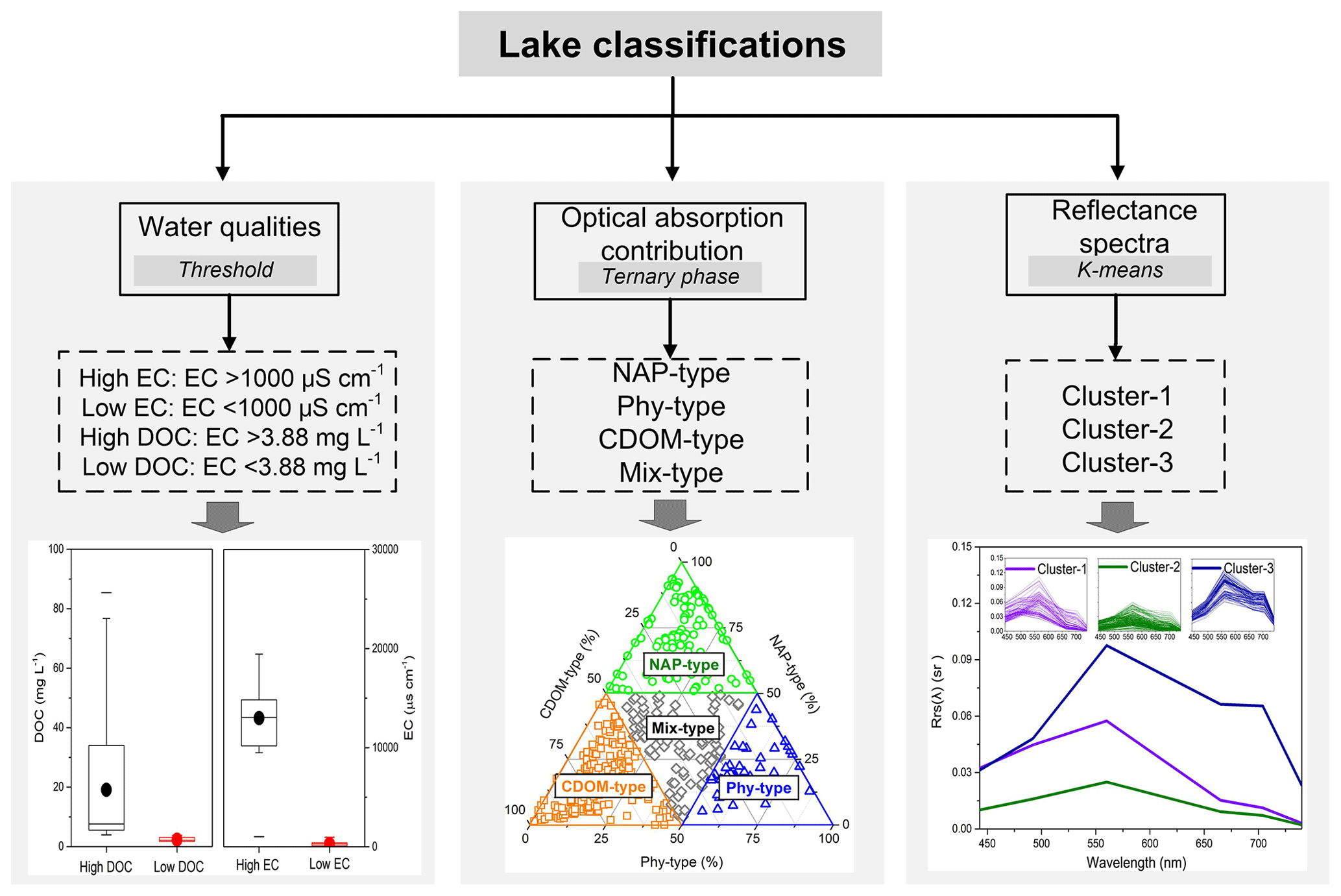
Figure 3 Lake classifications considering three types, i.e., water quality, optical absorption contribution and reflectance spectra. ANOVA analysis was conducted in different classifications (p<0.001) (Table S3).

2.7 Statistical analyses and accuracy assessment

Statistical analysis, including descriptive statistics, correlation (r), regression (R²) and ANOVA analyses, were implemented with the Statistical Program for Social Science software (version 16.0; SPSS, Chicago, IL, USA). Correlation and regression analyses were used to examine the relationships between the water quality parameters and absorption coefficients of OACs as well as the TSI model calibration and validation. The differences in trophic status, EC classification, DOC classification, absorption coefficients of OAC classification and MSI reflectance spectra classification for TSI model validation were assessed using one-way ANOVA. The significance level was set at $p<{\mathrm{0.05}}^{*}$. The mean normalized error (MAE) and root mean square error (RMSE) were used to assess the performance of the TSI model (S9–10).

3 Results

3.1 Aquatic environmental scenery

The water qualities and bio-optical properties of our samples covered a wide range, revealing different geographical environmental scenery (Tables S1 and S2–4). The EC and DOC concentration showed high variability, ranging, e.g., from 3345.31 µs cm⁻¹ (TuoSu, TS20) in the Tibet–Qinghai region to 0.17 µs cm⁻¹ (Qingnian, QN2) in the northeastern region. For the water quality parameters to characterize TSI, the Chl-a concentration ranged from 0.12 to 100.22 µg L⁻¹, with the highest value recorded in TaiPingChi (TPC5) and the lowest value in NamoCo (NMC36). The range of TP was from 0.003 mg L⁻¹ (Erlong, EL8) to 2.17 mg L⁻¹ (Dali, DL7), and SDD ranged from 0.17 m (Chalhu, CH32) to 9.47 m (NMC36) for surveyed lakes, respectively. Overall, the maximum values of EC, DOC, turbidity, Chl a, TSM and SDD were 196 782.35-, 948.4-, 723.3-, 770.92-, 614.58- and 55.71-fold greater than the minimum values, respectively, indicating that our dataset was representative of diverse water qualities.

Lake samples were grouped into different classifications based on water quality (e.g., EC and DOC), optical absorption contribution and reflectance spectra (Table 1 and Fig. 3). The results indicated that all water qualities showed significant differences (p<0.05) under different lake classifications. For example, brackish lakes showed higher average values of SDD, TP, DOC and optical attributions of OAC values than those of freshwater lakes, but the turbidity, Chl-a and TSM concentrations were lower. Lakes equipped with low DOC levels had a lower average value of SDD than that of lakes with high DOC levels. NAP-type lakes exhibited the highest average Chl-a and DOC values, whereas Phy-type lakes had the highest average turbidity and TSM values, and the highest average SDD and TP values were recorded in CDOM-type and mix-type lakes, respectively. For reflectance spectra classifications (Fig. 3), the highest average EC, SDD and DOC were recorded in cluster-1 lakes, the highest average turbidity and TP were shown in cluster-3 lakes, and the highest average TSM was found in cluster-2 lakes.

Table 1 (a) Averaged values (“Avg”) of water quality and bio-optical properties considering lake classifications and (b) ANOVA (F value) among them.

The unit of TN, TP, DOC and TSM is milligram per liter. The unit of EC is microseconds per centimeter. The unit of Chl a is microgram per liter. The unit of turbidity is NTU
(nephelometric turbidity unit). Significance levels are reported as significant, ^* 0.05 > p>0.01, or highly significant, ${}^{**}$ p<0.01.

3.2 Trophic status assessment

The trophic status of 45 lakes across China, from where in situ samples were collected, was evaluated (Fig. 4a). Our results showed that there were 13 oligotrophic (3.02 %), 199 mesotrophic (46.17 %) and 219 eutrophic (50.81 %) samples. Because our samples were collected in different seasons and eutrophication is time-dependent, the TSI values of samples within a lake were averaged. It can be shown that only 5 lakes accounting for 11.1 % of investigated lakes were characterized by an oligotrophic status, 17 lakes accounting for 37.8 % were mesotrophic, and 23 lakes accounting for 51.1 % were characterized by eutrophic status. These eutrophic lakes were distributed in the eastern region of China (Fig. 4b) and were associated with a highly concentrated human population and economic development. Moreover, the ANOVA results showed that the TSIs of lake samples were significantly different considering lake classifications (Fig. 4c and d).

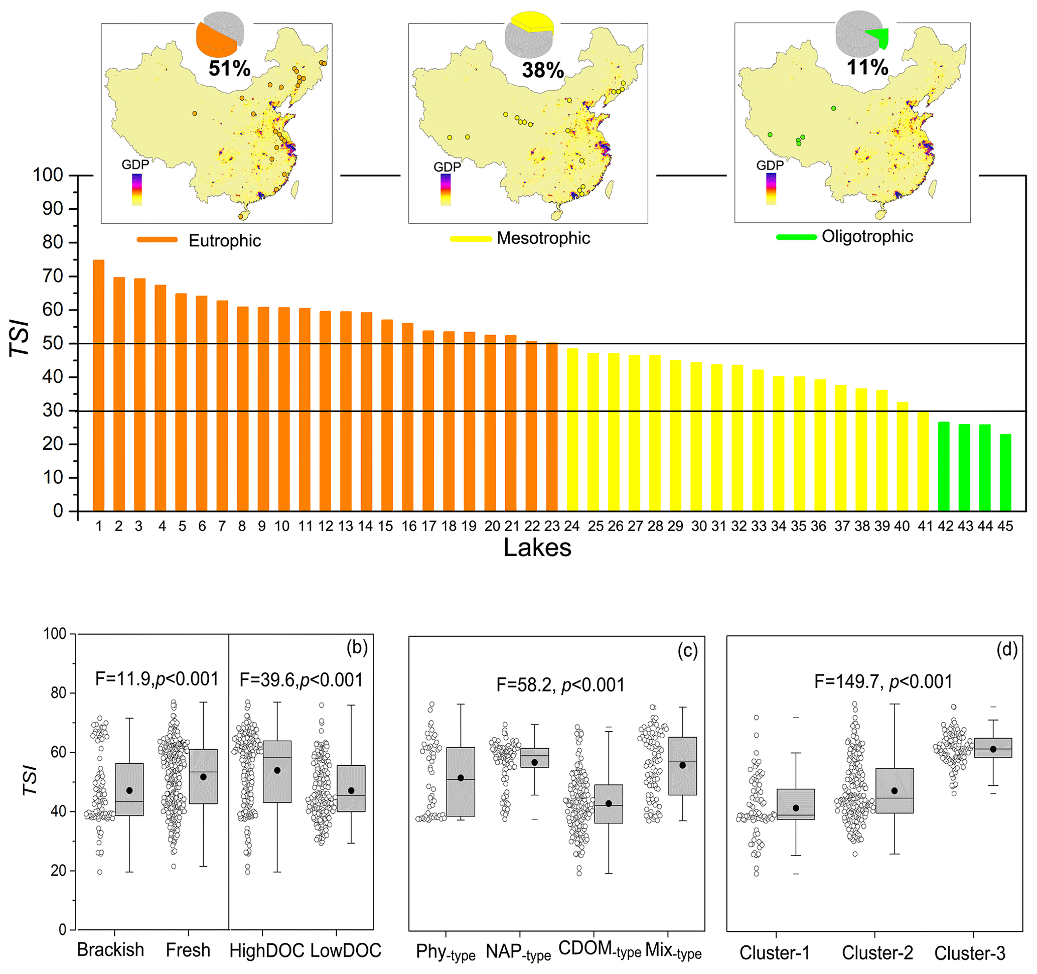
Figure 4 Panel (a) shows the averaged TSI in collected samples from lakes across China and their spatial distribution. The number of lakes can be found in Table S1. Box plots of the TSI for different classifications of water quality (b), optical absorption contribution types (c) and reflectance spectra (d). The balls beside the boxes are the lake samples, and the black balls in the boxes represent the mean values. The horizontal edges of the boxes denote the 25th and 75th percentiles; the whiskers denote the 10th and 90th percentiles.

3.3 Calibration and validation of the TSI model

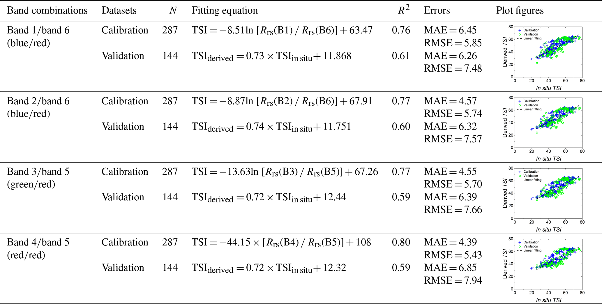
In this section, multiple linear regression was used to identify significantly sensitive spectral variables related to TSI (Table 2 and Fig. 2). Of the band combinations validated in the study (N= 144), the $\mathrm{blue}/\mathrm{red}$ $\left[R_{\mathrm{rs}}\left(\mathrm{443}\right)/R_{\mathrm{rs}}\left(\mathrm{740}\right),R_{\mathrm{rs}}\left(\mathrm{492}\right)/R_{\mathrm{rs}}\left(\mathrm{740}\right)\right]$ and $\mathrm{green}/\mathrm{red}$ $\left[R_{\mathrm{rs}}\left(\mathrm{560}\right)/R_{\mathrm{rs}}\left(\mathrm{704}\right),R_{\mathrm{rs}}\left(\mathrm{665}\right)/R_{\mathrm{rs}}\left(\mathrm{704}\right)\right]$ band ratios showed a good regression coefficient (R²>0.59) with TSI (Table S5). These band combinations provided certain sensitive spectral variables that responded to the lake eutrophic status. Hence, to strengthen the robustness of the three machine learning models, the $\mathrm{blue}/\mathrm{red}$ and $\mathrm{green}/\mathrm{red}$ combinations above were considered as input variables together with six spectral variables (R_rs(λ) at 443, 492, 560, 665, 709 and 740 nm). Likewise, the output variables were estimated using TSI to examine the performances (Fig. 5). The results showed that when XGBoost was applied to the validation data (N= 144), the performance of the model was excellent (R²= 0.87, slope = 0.85) with low errors (MAE = 3.15, RMSE = 4.11). The support vector machine (R²= 0.71, slope = 0.77, MAE = 4.67, RMSE = 6.11) and random forest (R²= 0.85, slope = 0.84, MAE = 3.31, RMSE = 4.34) models also showed significant performance. These results demonstrate the potential of using XGBoost by considering band combinations to derive TSI from Sentinel products.

Figure 5 Relationships between the in situ and derived TSI for both model training and testing samples by a support vector machine (a), XGBoost (b), random forest (c), as well as their errors (d).

Table 2 Multiple linear regression between the measured and estimated TSI from the MSI spectral bands after using the C2RCC processor.

3.4 TSI model application to lake classifications

The TSI model calculated by XGBoost was assessed by comparing derived and in situ TSI considering different lake classifications (Fig. 6). We aimed to provide a universal TSI model and evaluate its feasibility in different aquatic environments. Significant agreement (slope > 0.91, R²>0.91) between derived and in situ TSI was observed in lakes with high DOC levels (DOC > 3.88 mg L⁻¹) and EC values (EC > 1000 µS cm⁻¹) with low errors. For lakes classified by different absorption contributions, the NAP-type (slope = 0.98, R²= 0.88) and Phy-type (slope = 0.82, R²= 0.92) samples generally showed a more positive derived performance than those of Phy-type, CDOM-type and mix-type, respectively. In addition, a significant relationship between derived and in situ TSI can be described for lakes with cluster-1 reflectance spectra, with slope = 0.91, R²= 0.87, RMSE = 2.87 and MAE = 2.29.

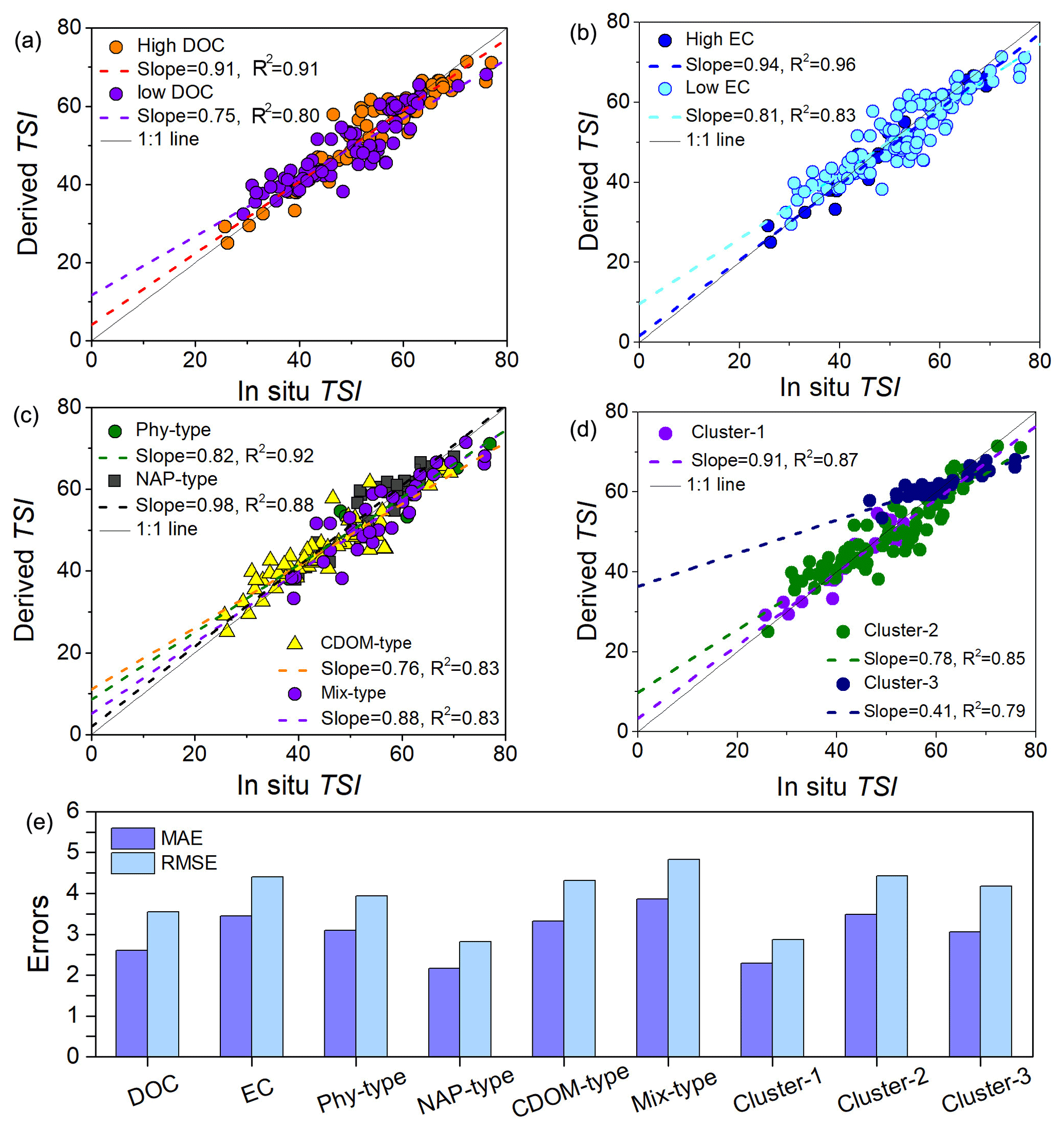
Figure 6 Scatter plots of the derived and in situ TSI by XGBoost for validation samples (N= 144) according to lake classifications, such as water quality (DOC and EC) (a–b), absorption contribution (c) and reflectance spectra (d) with the 1:1 line (solid red) and errors (e).

3.5 Spatial and seasonal patterns of trophic states: five lake limnetic regions

Previous studies have demonstrated that some lakes disappeared or increased numbers recently according to statistics from Ma et al. (2011). Thus, we selected some representative and stable lakes (N= 555) to qualify spatial trophic states using the XGBoost algorithm. The preprocessing of MSI data was referred to in Fig. 2, and a total of 139 cloud-free images in spring (April and May), summer (July and August) and autumn (September and October) covering the investigated lakes was acquired. According to the different geographic and limnological types in China, lakes were divided into five limnetic regions (Wang and Dou, 1998, Early National Investigation): the Eastern Plain Limnetic Region (EPLR, N= 123), Northeast Plain Limnetic Region (NPLR, N= 37), Inner Mongolia–Xinjiang Plateau Limnetic Region (IMXPLR, N= 56), Yungui Plateau Limnetic Region (YGPLR, N= 15) and Tibet–Qinghai Plateau Limnetic Region (TQPLR, N= 324) (Figs. 1 and S3).

In general, there were significant seasonal variations in the eutrophic state for lakes from the EPLR (F= 39.56, p<0.001) and TQPLR (F= 5.0, p<0.05) (Fig. 7). The averaged TSIs in EPLR were 56.37 (spring), 57.73 (summer) and 54.26 (autumn), indicating serious eutrophication of the investigated lakes consistent with the results from Li et al. (2022). Recognizing that over 94 % of the Chinese population lives in eastern watersheds with great demands of water use, this may be due to different water quality management on provincial scales. Likewise, we found that there was spatial heterogeneity of TSI results in TQPLR, some of which were the widespread saline lakes in the Qinghai–Tibet Plateau with high reflectance in satellite images. By contrast, there were no seasonal differences in TSI for lakes from IMXPLR, NPLR and YPLR, respectively. The eutrophic lakes dominated the proportions of the investigated lakes in the EPLR (93.5 %), followed by the NPLR (89.2 %), YGPLR (86.7 %), IMXPLR (69.6 %) and TQPLR (3.7 %) (Fig. 8). It was also found that mesotrophic lakes were found in the decreasing order of TQPLR (45.7 %), IMXPLR (30.4 %), YGPLR (13.3 %), NPLR (10.8 %) and EPLR (6.5 %), respectively. In comparison, most oligotrophic lakes (50.6 %) were distributed in the TQPLR.

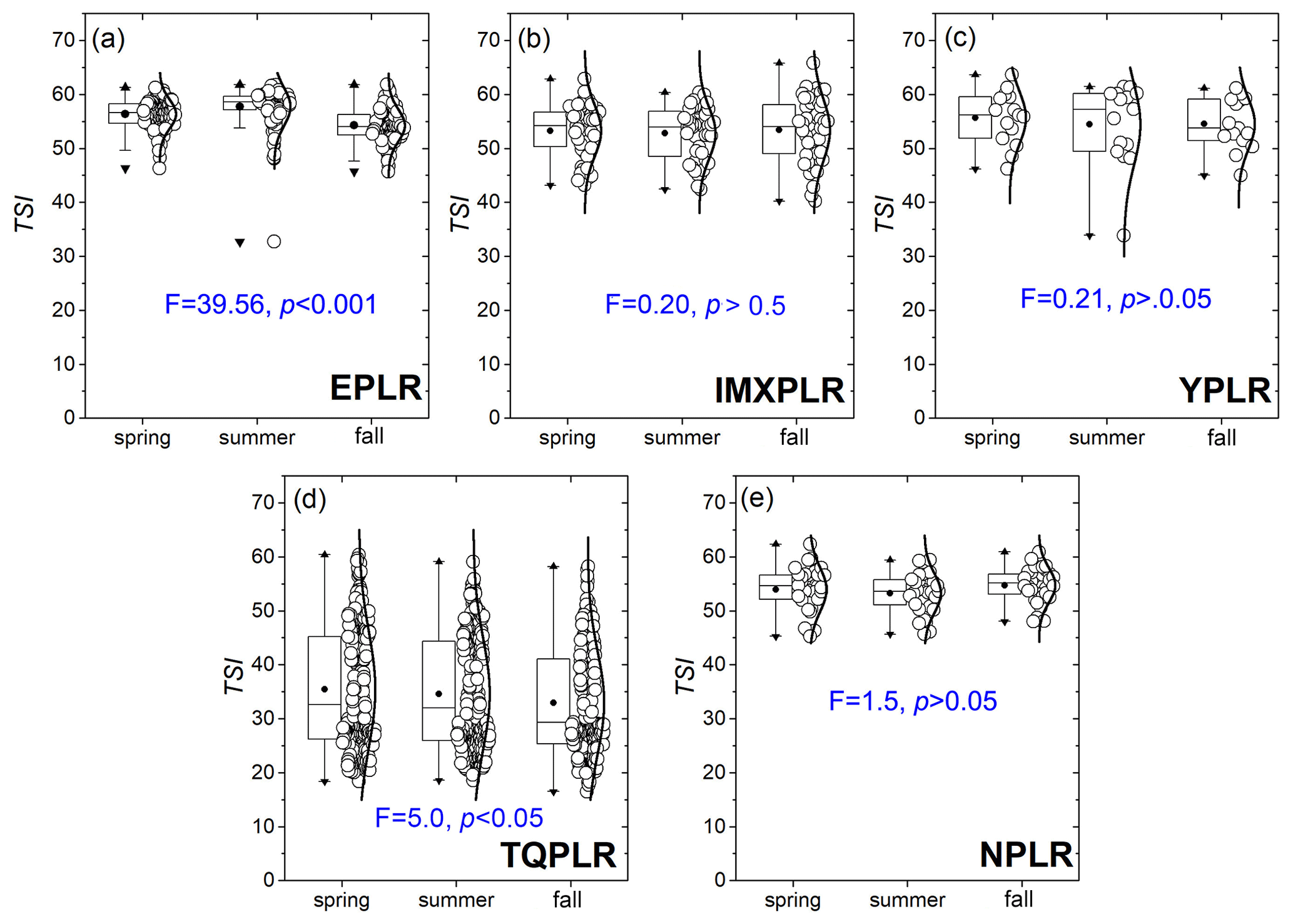
Figure 7 Box plots of the TSI derived from the XGBoost model in the investigated lakes from the five limnetic regions (Wang and Dou, 1998), i.e., (a) EPLR, (b) IMXPLR, (c) YPLR, (d) TQPLR and (e) NPLR. The black line and balls in the boxes represent the median and mean values, respectively. The horizontal edges of the boxes denote the 25th and 75th percentiles; the whiskers denote the 10th and 90th percentiles.

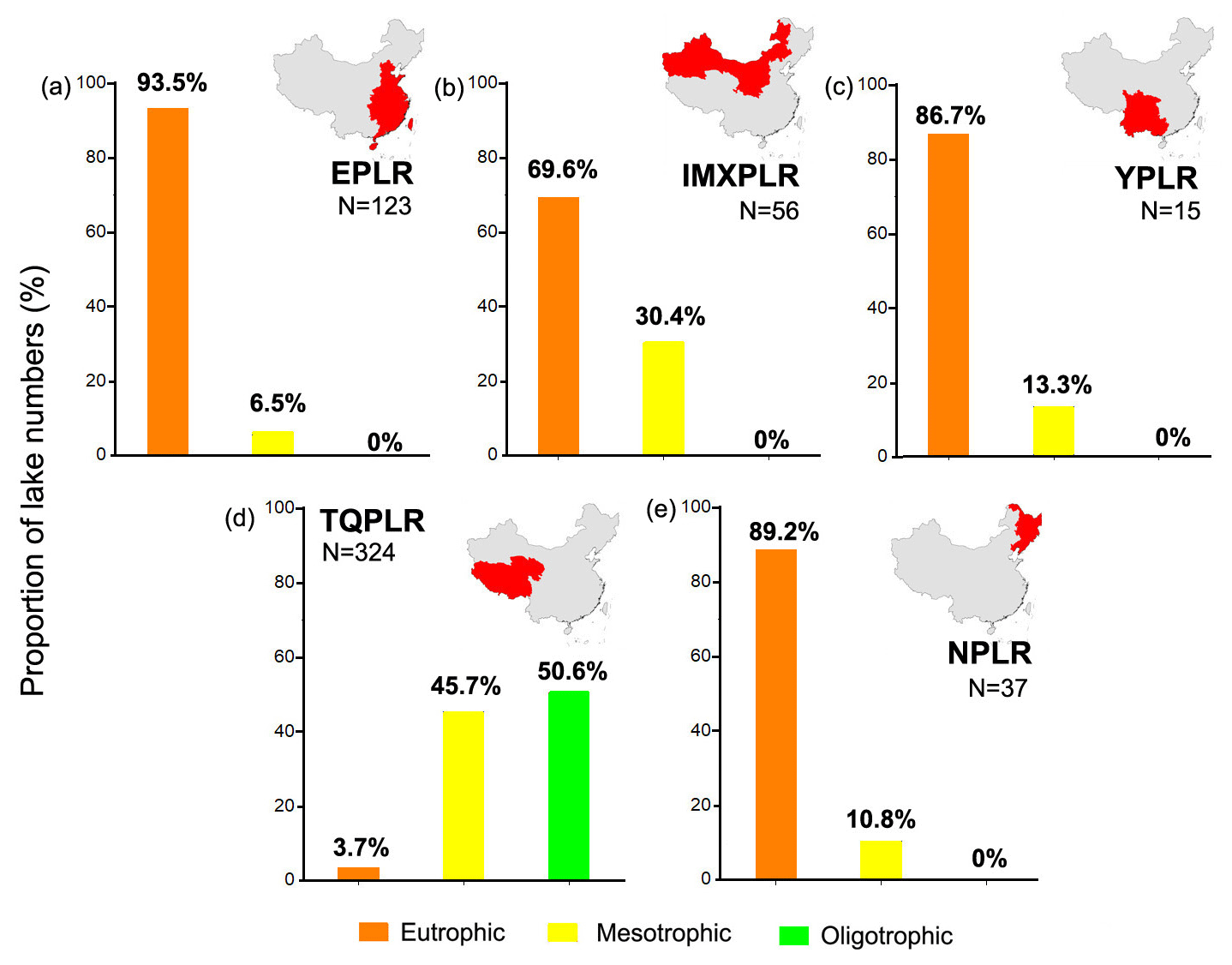
Figure 8 The proportions of lake numbers (%) for different trophic states in the five limnetic regions (Wang and Dou, 1998), i.e., (a) EPLR, (b) IMXPLR, (c) YPLR, (d) TQPLR and (e) NPLR. N represents the lake numbers.

4 Discussion

4.1 Remote-sensed and machine-learning-based TSI model

Traditional approaches to quantitatively characterize trophic status rely on field measurements of trophic parameters, e.g., Chl a, nutrients and SDD, to calculate TSI (Carlson, 1977). It is difficult and costly to make field measurements in lakes in remote locations. The TSI calculation does not need all of these trophic parameters, but just one, e.g., Chl a (Thiemann and Kaufmann, 2000), SDD (Olmanson et al., 2008; Song et al., 2020), TP (Kutser et al., 1995) and total absorption coefficients (Lee et al., 1999; Shi et al., 2019). There have been many lake studies (Chl a and SDD, Sheela et al., 2011; Chl a, SDD and TP, Song et al., 2012) where two or three water quality parameters were mapped, which would allow us to subsequently gather them to calculate a comprehensive TSI. Although these studies provided the potential to evaluate the trophic status of lakes, TSI is a synthetic indicator that is affected by biological, physical and chemical factors that co-vary in most instances. Huang et al. (2014) also tried to derive TSI using remote-sensing spectrum reflectance, but the accuracy was not completely usable. It shows that the variability in remote-sensing estimates of the TSI is not bad.

With advances in artificial intelligence technology and the increasing use of computer applications in recent years, machine learning has become a useful tool for monitoring aquatic environments by remote sensing (Mountrakis et al., 2011). It allows us to develop and evaluate a machine-learning-based TSI model that addresses quality and accuracy problems more effectively (Li et al., 2021). Hence, we propose a new approach to directly characterize the trophic status and accurately reflect spatial variations in this study, but this should also be conveniently available for the different lake classifications (Figs. 5, 6). Using machine learning algorithms, in order to improve the robustness and applicability of the TSI model, a sufficient database of trophic state parameters (N= 431) was collected from lakes with different biogeochemical characteristics, such as water quality, absorption contributions of different optically active substances and reflectance spectra (Table 1). We first used B1–B6 reflectances as input variables of machine learning algorithms, and XGBoost showed a significant performance with R² and a slope of 0.85 (Fig. S1). The SVM performed worse than XGBoost and random forest and did not produce sufficient performance. This is because the latter models are integrated algorithms with trees that are unpruned and diverse, signifying the high resolution in the feature space and the smoother decision boundary. There were no optical response bands or appropriate band ratios for TSI. We thus used a multiple linear regression to find some suitable sensitive band combinations responding to TSI, which made it possible to develop a robust machine-learning-based TSI model. It is important to note that the $\mathrm{blue}/\mathrm{red}$ $\left[R_{\mathrm{rs}}\left(\mathrm{443}\right)/R_{\mathrm{rs}}\left(\mathrm{740}\right),R_{\mathrm{rs}}\left(\mathrm{492}\right)/R_{\mathrm{rs}}\left(\mathrm{740}\right)\right]$ and $\mathrm{green}/\mathrm{red}$ $\left[R_{\mathrm{rs}}\left(\mathrm{560}\right)/R_{\mathrm{rs}}\left(\mathrm{704}\right),R_{\mathrm{rs}}\left(\mathrm{665}\right)/R_{\mathrm{rs}}\left(\mathrm{704}\right)\right]$ band ratios were significantly correlated with TSI (Table 2). This result indicated that the $\mathrm{blue}/\mathrm{red}$ and $\mathrm{green}/\mathrm{red}$ band ratios were more sensitive to TSI, although the nutrients and SDD had no optical response. It was known for decades that the blue part of the spectrum is useless when water itself is not blue (i.e., outside of the ocean or very oligotrophic mountain lakes), owing to the noneffective atmospheric correction and complex reflectance signals. However, our dataset to train TSI models contains the samples from blue and oligotrophic Tibetan lakes, which are like the oceanic environments (Liu et al., 2021). The blue bands responding to TSI were thus used in this study. Most empirical Chl-a estimation studies adopted red or near-infrared (NIR) band ratios to calibrate models using reflectance signatures (Gitelson et al., 1992). Similarly, empirical SDD retrieval models provided by previous studies that used empirical algorithms or models to figure out which bands should work best considered the following ratios: $\mathrm{blue}/\mathrm{green}$, $\mathrm{red}/\mathrm{blue}$ plus $\mathrm{red}/\mathrm{green}$, $\mathrm{red}/\mathrm{blue}$ plus blue (Bindling et al., 2007) and $\mathrm{Red}/\mathrm{Blue}$ plus blue (Kloiber et al., 2002). Kutser et al. (1995) also built a TP retrieval model using the red and NIR ratios, which is consistent with the Chl-a empirical models. Overall, it is not surprising for our TSI model to have strong correlations with the $\mathrm{blue}/\mathrm{red}$ and $\mathrm{green}/\mathrm{red}$ band ratios because the TSI incorporates the optical properties.

For this reason, we used MSI bands in the visible band ratios at six bands, considering the comprehensive spectrum information about the trophic status of lakes as an input variable (Fig. 2). The three representative machine learning TSI models improved the accuracy of the traditional linear regression (Table 2 and Fig. 5), and the results were better than those obtained with B1–B6 reflectances as input variables (Fig. S1). As a type of supervised machine learning algorithm, linear regression can be used to obtain certain learning criteria as expressions ($y=w_{\mathrm{0}}+w_{\mathrm{1}}\times x_{\mathrm{1}}+\mathrm{\dots }+w_{\mathrm{p}}\times x_{\mathrm{p}}$) of the optimal w_i solution. However, for complex targeted tasks, the fitting ability of linear regression is limited, and it cannot represent the real situation well. For example, a support vector machine can map data to another space, which can use a linear regression to distinguish the categories well. In complex environments (real world in machine learning), such as our large-scale database collected from different lakes (Fig. 1), there are various environmental factors as well as different seasons within a lake that have an impact on the trophic parameters and optical characteristics of lakes (Wen et al., 2016). Likewise, we found that the enhanced input variables, like the band ratios, if appropriately corrected for the TSI, resulted in a better performance (Fig. S1). This is consistent with some applications of machine learning algorithms (Cao et al., 2020) in which the performance of machine learning was reduced when covariances of input features were incorporated. This allows us to find more interesting TSI-correlated band ratios for MSI imagery in machine learning.

Several machine learning algorithms generally have different advantages and applicability owing to their different main principles (Cao et al., 2020; Li et al., 2021). This can be found in our results of the validation exercise, which showed that XGBoost provided stable TSI estimates, with a slope close to 1 and a good fitting coefficient of the measured and derived values (R²= 0.87, slope = 0.85, MAE = 3.15, RMSE = 4.11) (Fig. 4). Similarly, we can also find excellent performance (R²= 0.85, slope = 0.84, MAE = 3.31, RMSE = 4.34) for estimating TSI values by the random forest algorithm. This was likely because it is a summation of all weak learners weighted by the native log odds of error. In the case of boosting, we make decision trees into weak learners by allowing every tree to make only one decision before prediction (Chen et al., 2016). In some cases, XGBoost outperformed random forest. In addition, the support vector machine performed worse than XGBoost and random forest (Fig. 4). Li et al. (2021) used a support vector machine to estimate Chl-a concentrations with a relatively small dataset of 32 samples and 273 samples, respectively. This is consistent with the recent process in the development of support vector machines and has many advantages for remote-sensing applications with a small number of training datasets. Overall, the remote-sensing- and machine-learning-based TSI model aims to reduce the dependence of traditional field measurements while also providing a cost-effective approach to rapidly quantifying the trophic state.

4.2 TSI model for lake classifications

We validated the XGBoost TSI model considering different scenarios of lake classification, e.g., water quality, optical absorption contributions and reflectance spectra (Figs. 2 and 6). The results indicate three application scenarios for our model with low errors. The first one is of the XGBoost TSI model, which in particular performed well (slope > 0.91, R² > 0.91) in high-DOC (> 3.88 mg L⁻¹) and high-EC (> 1000 µS cm⁻¹) lakes (Fig. 6). We found that lakes with a high EC level correspondingly showed a high DOC level (Table 1), e.g., a high average EC value of 5156.02 µS cm⁻¹ and a high average DOC value of 18.75 mg L⁻¹ for NAP-type lakes. These brackish or saline lakes were distributed in the Tibet–Qinghai Plateau Region (e.g., KLK20, TS21, QHH22, SLC32, BMC34, ZRNMC36 or NMC37) and Inner Mongolia–Xinjiang Plateau Limnetic Region (e.g., DL8, HSH10, DH17, HL18 or WLSH16) (Table S1). Our results are in agreement with those of previous studies that the DOC and EC of inland waters located in semi-arid regions can be attributed to the evapoconcentration and accumulation processes (Curtis and Adams, 1995) as well as anthropogenic activities. Further, it can be observed that oligotrophic lakes accounting for 11.1 % were also distributed in the Tibet–Qinghai Plateau Region (Fig. 4).

Secondly, we found that our XGBoost TSI model performed well if the trophic parameters that correlated with the TSI_M(Chl a) or TSI_M(SDD) dominated the lake classifications. Specifically, the high Chl-a (averaged 14.26 µg L⁻¹) and a_ph(440) (averaged 0.26 m⁻¹) levels in NAP-type lakes showed the best performance (slope = 0.98, R²= 0.88) over those of other optical absorption contribution classifications (Fig. 6). In fact, there was a negligible difference in the performance for application in Phy-type and NAP-type lakes. For the third scenario, for the reflectance spectrum classification, cluster-1 lakes with low TSM (averaged 5.76 mg L⁻¹), turbidity (averaged 4.46 NTU), and a_d(440) (averaged 0.26 m⁻¹) levels and a high SDD level (average 2.38 m) also showed good performance (slope = 0.91, R²= 0.87) (Fig. 6). In general, TSI, as a comprehensive index incorporating the optical properties of itself, was calculated using trophic state parameters: TSI_M(Chl a), TSI_M(SDD) and TSI_M(TP) in Eq. 7. Our XGBoost TSI model performed best in the present study, which confirmed that the performance was mostly determined by biogeochemical environments in larger-scale regions. We cannot explain the dependence of the TSI model on the physico-optical properties. From another point of view, it can be inferred that the XGBoost TSI model applications mostly correlated with the Chl a and SDD because of their high weight allocation in the TSI equation.

Although we conducted a large-scale TSI observation across Chinese lakes, whether or not XGBoost could also perform well for a signal lake should be evaluated. Hence, the in situ measured samples were classified in three scenarios, and the XGBoost TSI model was analyzed. Overall, in future work, for lakes mainly located in a high-elevation and arid region with high DOC or EC levels, the input band combinations responding to CDOM ($\mathrm{Green}/\mathrm{Red}$) could be added to the XGBoost TSI model. This is because the CDOM and DOC generally showed positive correlations for investigated lakes (Song et al., 2013b), and CDOM is one of the optical active substances. This also confirmed that non-algal particles could cover the reflectance signals and impact the model performance in the second and third scenarios. More classifications based on reflectance spectra (Spyrakos et al., 2018) and the water color index (Wang et al., 2018) should first be used and corresponding models for high-turbidity lakes then developed.

4.3 Trophic status in five limnetic regions

According to this study, more than 50 % of lakes were eutrophic, indicating a long-standing status of eutrophication (Fig. 4), as seen by the mapping of 555 lakes by our XGBoost TSI model (Fig. 7). Some lake investigations undertaken earlier in China concluded that during 1978–1980 41.2 % of lakes were eutrophic in China (Jin and Hu, 2003), during 1988–1992 51.2 % of lakes were eutrophic (Wang and Dou, 1998), during 2001–2005 84.5 % of lakes were eutrophic, and during 2011–2019 50 % of lakes (Wen et al., 2019) were eutrophic or undergoing eutrophication. In our study, some historical records of Chl a, SDD and TP from a comparison to an earlier national investigation by Wang and Dou (1998) were collected in typical lakes, e.g., Lake Dongting, Lake Poyang, Lake Chaohu, Lake Taihu and Lake Jingpo, respectively (Table S6). Evidently, Chinese lakes have deteriorated considerably in terms of water quality at an alarming rate for typical lakes, e.g., Lake Jingpo, Lake Dongting and Lake Poyang, during the past ∼ 22 years (Table S6). Lake eutrophication is influenced by both natural (hydrological processes, topography, lake depth and buffer capacity) factors as well as anthropogenic factors (land-use changes, urbanization construction as well as domestic and industrial pollution) (Müller et al., 1998). A large-scale overview of lake eutrophication indicated that there was a significant difference (ANOVA, F= 255.2, p<0.001) in the five limnetic regions (Wang and Dou, 1998). Owing to the imbalanced development of the economy (Fig. S2, gross domestic product and population), geological topography (Fig. S3, solar radiation intensity and sunshine hours) and climate (Fig. S4, annual temperature and precipitation), it was not surprising that the eutrophic lakes were generally distributed in the Eastern Plain Limnetic Region and Northeast Plain Limnetic Region nor that the oligotrophic lakes were found in the Tibet–Qinghai Plateau Limnetic Region (Figs. 4 and 7).

Considering the natural factors for the distributions of Chinese lake eutrophication, we could suppose some possibility that lake depth and lake hydrological processes cause the eutrophication of lakes in China. Previous studies (Wang and Dou, 1998; Huang et al., 2014) have demonstrated that lakes with mean depths > 5 m in China are mainly located in the Yungui Plateau Limnetic Region, Inner Mongolia–Xinjiang Plateau Limnetic Region and Tibet–Qinghai Plateau Limnetic Region, whereas almost all lakes located in the Eastern Plain Limnetic Region are shallow. Both these lakes in the Eastern Plain Limnetic Region are hydraulically connected with the Yangtze River, with a temporary residence time of approximately 30 d (Fig. S7). In shallow lakes, due to wind waves or disturbance by fishes, the phosphorus and nitrogen nutrients stored in the sediment can be easily resuspended and released into the overlying water (Niemistö et al., 2008). Consequently, an increased frequency of algal blooms can be found in the Eastern Plain Limnetic Region in lakes such as Taihu, Chaohu and Hongze (Qin et al., 2019; Yao et al., 2016). Instead, deeper lakes, such as the ones in the YGPLR and TQPLR, possess a relatively good buffer capacity for wastewater runoff (Huang et al., 2014). Carvalho et al. (2009) found that Chl-a levels decreased with lake water depth and geographic location. Qin et al. (2020) and Tong et al. (2006) demonstrated that phosphorus reduction can mitigate eutrophication in deep lakes, and more efforts to reduce both N and P need to be undertaken in shallow lakes. This can be demonstrated in our case of Lake Fuxian with changeable eutrophication levels, with an average depth of 87 m, which was the deepest lake in southwestern China (Fig. S7). In addition, the annual precipitation and air temperatures were relatively high in the EPLR (Fig. S4). Hydrological and meteorological processes can scour land surfaces and bring nutrients into lakes via rivers. Therefore, lake ecosystems were strongly related to the lake basin morphology and its hydrologic characteristics, which were higher in shallow lakes than in deep ones (Köiv et al., 2011).

On the other hand, human-induced eutrophication, e.g., agricultural fertilization (Carpenter et al., 2008; Huang et al., 2017), aquaculture (Guo and Li, 2003) and sewage discharge (Paerl et al., 2011), is increasing terrestrial nutrient phosphorus but not nitrogen concentration inputs (Schindler et al., 2008). We suspected that two interactive factors, such as land-use and nutrient variations, cause lake eutrophication, because this can be found in our investigation of distributed lakes in the EPLR in comparison to an earlier national investigation by Wang and Dou (1998). Many lakes in the EPLR that were naturally connected with rivers have been modified to paddy fields, and some small lakes have become isolated for lake aquaculture. For instance, Lake Dongting was artificially shifted from being river-fed to being dammed or isolated. Logically, a dam should settle suspended matter and nutrients via river inputs. However, the shallow characteristic and wind-mixing influence process significantly increased the probability of eutrophication (Liu et al., 2019). In the EPLR and NPLR, 94 % of China's population lives in 43 % of its eastern region, which visually demonstrates the distribution of the gross domestic product (GDP) with a densely populated east (Fig. S2). Owing to the requirements of water source utilization, the EPLR has lost one-third of its original lake areas to cropland since 1949 (Yin and Li, 2001). Lake aquaculture is highly active in these areas. These processes could lead to terrestrial nutrient loading into lakes, from either agriculture or aquaculture, and thereby alter the trophic state levels of a lake ecosystem. In 2019, the total fish catch in Hubei was 4695 t, in Jiangxi it was 432, 25 t, in Anhui it was 588 135 t, and in Anhui and Jiangsu it was 2 314 603 and 4 841 159 t in the east, respectively (China Rural Statistical Yearbook, 2021).

Although we have not systematically analyzed the effects of environmental factors on trophic status, some of the sparse existing comparative literature supported certain spatiotemporal patterns. It should be emphasized that China has been facing serious lake eutrophication and unbalanced distributions. Almost invariably, lake ecosystem health would still be impacted by stresses integrating anthropogenic and overexploitation of catchment resources. Consequently, addressing the issue of worsening eutrophication will require a better understanding of the environmental interactive mechanisms in the future.

4.4 Limitations, uncertainties and future

In pursuit of the United Nation's Sustainable Development Goal (SDG) 6.3.2, satellite imagery and machine learning still provide great potential for evaluating water quality states from global observations, particularly in developing countries. Machine learning algorithms could serve as good alternatives for empirical and semi-analytical algorithms to quantify large-scale spatial applications, which could avoid or minimize the errors. Our results further demonstrated that machine learning algorithms could improve the accuracy of water quality models (e.g., TSIs) when the linear regression was used to find sensitive band combinations with $\mathrm{red}/\mathrm{red}$ edge bands. Previous studies (Li et al., 2021, 2022) found that a $\mathrm{red}/\mathrm{red}$ edge band could help us to quantify the spatial and temporal changes in Chl-a concentration or a synthetic parameter – such as TSI with a high Chl-a weight ratio – from regional lakes. It enables us to use Sentinel-2 or similar sensors equipped with these bands to capture records of TSI dynamics.

As a medium-resolution (10–60 m) satellite, Sentinel-2 MSI offers the potential to monitor small-sized lakes and produce reliable TSI estimates. However, there are significant obstacles in generating a Sentinel-2 (∼ 10 m) lake TSI distribution, including the acquisition of high-quality atmospheric-corrected R_rs(λ) and massive computational overhead by the C2RCC processor (Li et al., 2023). The C2RCC processor designed for waters based on neural networks is a data-driven approach and uses huge datasets collected from in situ and simulation measurements. In situ reflectance measurements were not conducted in these investigated Chinese lakes when sampling. Our recently study reported that the C2RCC (SNAP 8.0) and Polymer (v4.13) processors both performed best with in situ field radiometry in typical lakes across China (Li et al., 2023), but the latter could work better when all bands are pooled together in derived algorithms. Considering the growing requirements of TSI products, more in situ measurements would be required to be added to the already-implemented processors in future work.

In addition, there is a need for a robust model developed from different locations and optical water types that accounts for the interplay of different water quality parameters. The machine learning TSI model required a highly calibrated dataset, including high nutrients (e.g., TP > 2.50 mg L⁻¹ in this study) and Chl-a concentrations (> 100 µg L⁻¹ in this study). Likewise, for our developed universal TSI model, the feasibility application performances were different considering lake classifications. Hence, the extensive field–lab materials with complex source variations would be required first, and water optical typologies further are a good compromise to develop groups of optimized algorithms in the future. Nevertheless, we aim to provide a technical operation approach that could prompt more analysis responding to warming climate and anthropogenic activities. The strong linkages between reflectance and several trophic states defining indexes further underscore the potential of remote sensing for resource-limited countries to meet their SDG goals.

5 Conclusions

Our study presents a novel remote-sensing- and machine-learning-based algorithm that allows us to retrieve lake TSI from Sentinel-2 MSI imagery. We used a match-up database (N= 431) over a diverse range of bio-optical regimes to train machine learning algorithms and validated it against in situ data. The trophic states of 555 lakes were then evaluated. These results provide a better understanding of how remote-sensing- and machine-learning-based models allow us to estimate eutrophication over a large scale of different lakes. Our main findings can be summarized as follows.

1. Linear regression enabled us to find certain band combinations sensitive to TSI (R²>0.59), e.g., the $\mathrm{blue}/\mathrm{red}$ $\left[R_{\mathrm{rs}}\left(\mathrm{443}\right)/R_{\mathrm{rs}}\left(\mathrm{740}\right),R_{\mathrm{rs}}\left(\mathrm{492}\right)/R_{\mathrm{rs}}\left(\mathrm{740}\right)\right]$ and $\mathrm{green}/\mathrm{red}$ $\left[R_{\mathrm{rs}}\left(\mathrm{560}\right)/R_{\mathrm{rs}}\left(\mathrm{704}\right),R_{\mathrm{rs}}\left(\mathrm{665}\right)/R_{\mathrm{rs}}\left(\mathrm{704}\right)\right]$ band ratios.

2. The XGBoost algorithm resulted in optimum performance with R²= 0.87 and slope = 0.85, considering the low errors (MAE = 3.15, RMSE = 4.11), compared to the support vector machine and random forest algorithms.

3. If there are some preliminary data available from the study area, one can improve the performance of the machine learning by dividing the lakes based on high DOC or EC, NAP-type, Phy-type and cluster-1 reflectance spectra.

4. The trophic states of 555 lakes were evaluated in five limnetic regions: eutrophic lakes dominated in the Eastern Plain Limnetic Region and Northeast Plain Limnetic Region, and most lakes in the Tibet–Qinghai Plateau Limnetic Region were mesotrophic or oligotrophic.

In our subsequent research and management, qualification and mapping of TSI will be implemented as a remote-sensing and machine learning model in a large-scale study, allowing for improved performance. In the future, Sentinel-2 MSI data could be used to reveal spatiotemporal variations in lake trophic states in long-term time series responding to climate and anthropogenic activities.