the Creative Commons Attribution 4.0 License.
the Creative Commons Attribution 4.0 License.
 | 28 Sep 2023
Technical note: Novel analytical solution for groundwater response to atmospheric tides
Jose M. Bastias Espejo
Chris Turnadge
Russell S. Crosbie
Philipp Blum
Gabriel C. Rau
Subsurface hydraulic and geomechanical properties can be estimated from well water level responses to Earth and atmospheric tides. However, the limited availability of analytical solutions restricts the applicability of this approach to realistic field conditions. We present a new and rigorous analytical solution for modeling flow between a subsurface–well system caused by harmonic atmospheric loading. We integrate this into a comprehensive workflow that also estimates subsurface properties using a well-established Earth tide method. When applied to groundwater monitoring datasets obtained from two boreholes screened in a sand aquifer in the Mary–Wildman river region (Northern Territory, Australia), estimated hydraulic conductivity and specific storage agree. Results also indicate that small vertical leakage occurs in the vicinity of both boreholes. Furthermore, the estimated geomechanical properties were within the values reported in the literature for similar lithological settings. Our new solution extends the capabilities of existing approaches, and our results demonstrate that analyzing the groundwater response to natural tidal forces is a low-cost and readily available solution for unconsolidated, hydraulically confined, and undrained subsurface conditions. This approach can support well-established characterization methods, increasing the amount of subsurface information.
- Article
(4287 KB) - Full-text XML
- BibTeX
- EndNote


Knowledge of subsurface hydrogeomechanical properties is crucial for Earth resource development and management. Such properties determine the capacity of hydrostratigraphic units to store and transmit groundwater. Traditional, active hydraulic testing methods such as pumping, slug, pressure, and packer tests or laboratory analyses of cores involve considerable logistical expenses (Maliva, 2016). In contrast, passive methods (e.g., tidal subsurface analysis, TSA), which are used to estimate hydraulic properties from well water level responses to ubiquitous periodic forces (Merritt, 2004; Cutillo and Bredehoeft, 2011), are relatively low cost to implement and derive additional values from commonly measured datasets (McMillan et al., 2019; Rau et al., 2020, 2022). The effect of gravitational effects and atmospheric loading on the subsurface has long been observed and reported (Meinzer, 1939) and is contained in routine groundwater pressure measurements made in countless observation wells around the world (McMillan et al., 2019). The influence of natural forces such as tides on groundwater pressures is ubiquitous, allowing widespread applications reducing the effort and cost of investigations. Since passive approaches rely on natural signals and do not require any active perturbation of the subsurface system, we will refer to them collectively as passive subsurface characterization (PSC) in our work.
Earth and atmospheric tides act as harmonic forces at various frequencies (McMillan et al., 2019). For groundwater investigation the most informative frequencies range from 0.8 to 2.0 cpd (cycles per day) (Merritt, 2004). The dominant frequencies present in groundwater pressure measurements are O1 (0.9295 cpd), M2 (1.93 cpd), and S2 (2.00 cpd). These components generally show a higher amplitude in comparison with other tidal harmonics and are, therefore, more likely to be contained in field datasets (McMillan et al., 2019).
Loading forces cause mechanical deformation of the water-saturated porous medium, leading to an instantaneous pore pressure response and a hydraulic gradient towards the nearby observation well. This gradient drives groundwater exchange between the subsurface and the well until re-equilibrium is achieved (Cheng, 2016; Verruijt, 2013; Wang, 2017). The amplitude ratio between the magnitude of well water level variation and subsurface pore pressure variation, as well as the time delay required for groundwater exchange, expressed as a phase shift or phase lag, can be used to estimate subsurface hydrogeomechanical properties (Hsieh et al., 1987). Positive phase shifts (i.e., when well water levels respond before subsurface water pressures to Earth-tide-induced strain variations) have been linked to vertical connectivity with adjoining hydrostratigraphic units (Roeloffs et al., 1989) and negative skin effects of the observation well (Valois et al., 2022). Amplitude ratios and phase shifts can be readily extracted from measurements and inverted using established analytical solutions (McMillan et al., 2019).
Cooper et al. (1965) derived an analytical solution for the movement of groundwater caused by seismic waves in fully confined aquifers. Bredehoeft (1967) proposed a method to interpret the effect of Earth tides on observation wells based on classic solid mechanics, which allowed the estimation of specific storage of the aquifer if the Poisson ratio of the porous medium was known. However, this method did not comply with Biot consolidation theory (Biot, 1941), as it did not couple fluid dynamics with mechanical deformation. Subsequently, many studies described the effect of Earth tides in poroelastic systems (Bodvarsson, 1970; Robinson and Bell, 1971; Arditty et al., 1978; Van der Kamp and Gale, 1983) but did not consider the damping effect of the observation well on the amplitude and phase. To address the signal-diminishing effect of a well, Hsieh et al. (1987) combined the poroelastic response of a confined aquifer with the work of Cooper et al. (1965) and derived an analytical solution to model flow to wells due to Earth tides.
Rojstaczer (1988) proposed an analytical solution for modeling flow to wells induced by atmospheric tides. However, the solution requires knowledge of vadose properties which are often unknown, and it does not account for the effect of barometric efficiency on confined pore pressure (also known as tidal efficiency). To address this, Rojstaczer and Riley (1990) developed an analytical solution that includes the barometric effects on confined pore pressure, but it does not consider the effects on the amplitude and phase shift of a well. Additionally, the mean stress in their formulation only considers the vertical direction and neglects lateral directions, which can lead to significant errors for typical Poisson ratio values (Cheng, 2016; Verruijt, 2013; Wang, 2017).
Several studies have estimated subsurface properties using Earth tide analysis (Le Borgne et al., 2004; Doan et al., 2006; Cutillo and Bredehoeft, 2011; Lai et al., 2013, 2014; Rahi and Halihan, 2013; Xue et al., 2016; Shi and Wang, 2016; Acworth et al., 2016). However, many of the analytical solutions used to derive estimates assume oversimplified settings, which can lead to inaccurate results. To address this, Wang et al. (2018) recently developed an analytical solution that describes flow in and out of a well caused by Earth tides in a two-layered flow system. Gao et al. (2020) accounted for the well skin effect, which occurs when the physical properties of the formation in a larger area around a borehole are affected by drilling, leading to a reduced amplitude ratio and phase shift. Additionally, Guo et al. (2021) derived an analytical solution to describe flow in fractures caused by Earth tides and estimated hydraulic properties. Finally, Liang et al. (2022) solved the Richards equation (Freeze and Cherry, 1979) to include the effect of the unsaturated zone, finding that it delays the phase shift response of the borehole pressure.
Xue et al. (2016) and Rau et al. (2020) used the analytical solution of Wang (2017) to model the barometric effect of atmospheric tides with vertical leakage, but it lacks the damping effect of an observation well. Recently, Rau et al. (2022) proposed a new approach based on the work of Acworth et al. (2017) that combines poroelastic relations for one-dimensional Earth and atmospheric tide deformation to obtain a system of equations with poroelastic properties. However, their approach is based on an analytical model that does not correctly represent vertical leakage. To the best of our knowledge, there is no rigorous analytical solution in the literature to model flow to wells induced harmonically from atmospheric tides based on the mean stress flow equation while considering a semi-confined aquifer.
The objective of this work is twofold. Firstly, we introduce a new analytical solution based on the Biot theory of consolidation that describes the flow in a subsurface–well system caused by the harmonic loading of atmospheric tides. Secondly, we demonstrate its usefulness by applying it to well water levels from two boreholes in the Northern Territory of Australia and comparing the results with established Earth tide methods and existing knowledge of the groundwater system. Our study demonstrates that our new analytical solution extends the range of properties that can be accurately estimated and provides a better understanding of subsurface processes and properties.
In this section, a new analytical solution based on the mean stress flow equation is derived to simulate flow to wells resulting from atmospheric tides loading the surface. The fluid continuity equation in the mean stress form can be used to describe the water flow from a semi-confined aquifer towards an observation well. If only radial flow is assumed and small vertical fluid exchange from the semi-confined layer occurs, the equation reads as (Cheng, 2016; Verruijt, 2013; Wang, 2017)
Here, t represents time, and σ is the mean stress. K is the drained bulk modulus of the solid material. r is the radius. The hydraulic head of the fluid (groundwater for this study), h, is used as a proxy for pore pressure pf=ρgh. T is the transmissivity of the aquifer with T=kaHa, where ka is the hydraulic conductivity and Ha is the aquifer thickness. If the aquifer is overlain by a leaky aquitard, then the downward leakage flux can be described as , where kl is the vertical hydraulic conductivity and Hl is the aquitard-saturated thickness. Note that this approximation is only valid when . α is the Biot coefficient that is equal to one for unconsolidated systems (e.g., gravels, sands, and clays) and has the range for consolidated systems (e.g., bedrock) where n is the effective porosity. Sσ is the Biot modulus at constant stress (also known as a three-dimensional storage coefficient) (Cheng, 2016; Verruijt, 2013; Wang, 2017).
where g is gravitational acceleration (9.81 m s−2) and ρ is the fluid density (1000 kg m−3). R is the Biot modulus at constant stress defined as (Cheng, 2016; Verruijt, 2013; Wang, 2017)
where Kf is the bulk modulus of the fluid ( Pa for freshwater).
Barometric pressure fluctuations cause loading at the ground surface, which results in vertical deformation of the subsurface and, therefore, changes to the internal stress balance of the fluid–solid skeleton system. For example, when atmospheric pressure rises, the formation undergoes compressive stress, resulting in an increase in the confined pore pressure (Domenico and Schwartz, 1997). If a change in pore pressure is only caused by a vertical loading and only vertical deformation is allowed, the mean stress can be computed as
In a fully saturated porous medium, this effect can be described by Biot consolidation theory as follows (Cheng, 2016; Verruijt, 2013; Wang, 2017):
Here, pf is the fluid (i.e., water in this study) pore pressure. σ is the mean stress. K is the drained bulk modulus of the solid material. ξ is the change in fluid content and can be used to quantify changes in pore pressure resulting from hydraulic gradients (Cheng, 2016; Verruijt, 2013; Wang, 2017). The sign of this parameter indicates whether a fluid is leaving or entering a given porous medium.
Biot consolidation theory assumes ξ=0 when undrained conditions apply within the porous medium (Cheng, 2016; Verruijt, 2013; Wang, 2017). Conversely, system conditions are drained when ξ≠0. Note here that a drained porous medium differs conceptually from a confined aquifer, and these concepts are often mixed up in the literature. For example, a confined aquifer may exchange fluid via one of its horizontal boundaries, such as a confined aquifer bounded by a river.
Assuming undrained conditions (ξ=0) and an unconsolidated system (α=1), we solved Eq. (1) for steady-state conditions to obtain the periodic water level in an open borehole. This assumes that the instantaneous mechanical equilibrium requires the loading period to be long relative to the times for elastic wave propagation. Furthermore, the initial transient state when the surface loading starts is neglected. Under this pseudo steady-state approximation, i.e., time and depth are independent, the solution is first order and has the form due to atmospheric loading, where ω is the angular frequency of the tide signal and superscript “AT” stands for atmospheric tide, e.g., S1 at 1 cpd or the atmospheric response to S2 at 2 cpd (Merritt, 2004; McMillan et al., 2019).
As a boundary condition, the hydraulic head far away from the radius of influence of the borehole is given only by the mechanical response of the system:
where r∞ is a distance far away from the radius of influence of the borehole, and the hydraulic head at the borehole screen, hw, should be the water level in the bore:
The bore and the aquifer are free to exchange groundwater; i.e.,
With these boundary conditions, the solution of the water level in the borehole is derived as
where the periodic atmospheric loading is assumed to be only vertical (i.e., σ=σzz), modeled as σ=σatmeiωt. Thus, σatm represents the amplitude of the atmospheric tide, and
Here, K0 and K1 are the modified Bessel functions of the second kind and orders zero and one, respectively, and
Note that Sϵ, the specific storage at constant strain, and Sσ are related as (Cheng, 2016; Verruijt, 2013; Wang, 2017)
Since it is assumed that the borehole is open to the atmosphere, any change in barometric pressure will also play a role in the hydrostatic pressure inside the borehole. Thus, the amplitude ratio between the atmospheric loading and the confined pore pressure due to atmospheric tides, AAT, has to be expressed as the balance between the far-field pore pressure (, Eq. 5), the amplitude of the atmospheric load (σatm(ρg)−1), and the change in fluid level in the well, hw,o, such that
The time lag between the far-field-confined pore pressure and the actual change in fluid in an open well is given by
Note that the applied amplitude of the periodic stress at a boundary has to be equal to the atmospheric pressure:
where Patm is the barometric pressure measured in the field. In this convention, the compression stress is opposite in sign compared to the atmospheric pressure as an increase compresses the subsurface.
We have named our novel analytical solution the mean stress solution. Drawing an analogy with established Earth tide methods (Hsieh et al., 1987; Wang et al., 2018, e.g.,), our new solution enables the estimation of subsurface hydraulic and geomechanical properties from atmospheric tidal components that are ubiquitous in standard field measurements of well water levels. This innovative solution expands the scope of existing approaches that passively characterize subsurface processes and properties (McMillan et al., 2019).
3.1 Field site and groundwater monitoring
In this section, we apply our analytical solution to field data, compare the results with those derived from established Earth tide methods, and consider the results in the context of existing knowledge such as from lithological logs and hydraulic testing. The overall workflow applied in this section is shown in Fig. 1, which incorporates established Earth tide methods alongside our new solution.
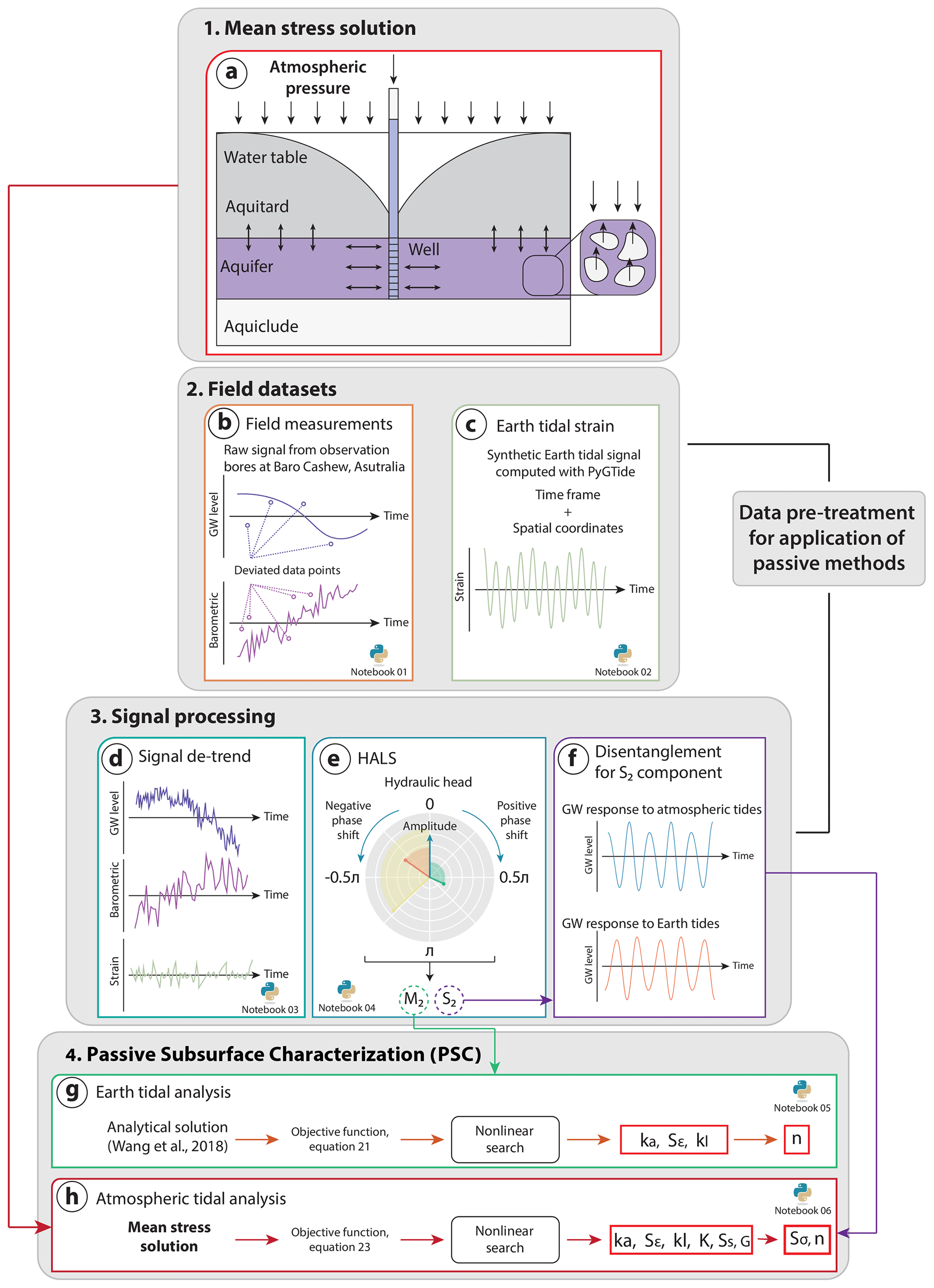
Figure 1Overview of the workflow applied to estimate subsurface hydraulic and geomechanical properties using the groundwater response to Earth and atmospheric tides. The dataset and Python scripts developed for this work are available in an external repository (see the Code and Data availability statements).
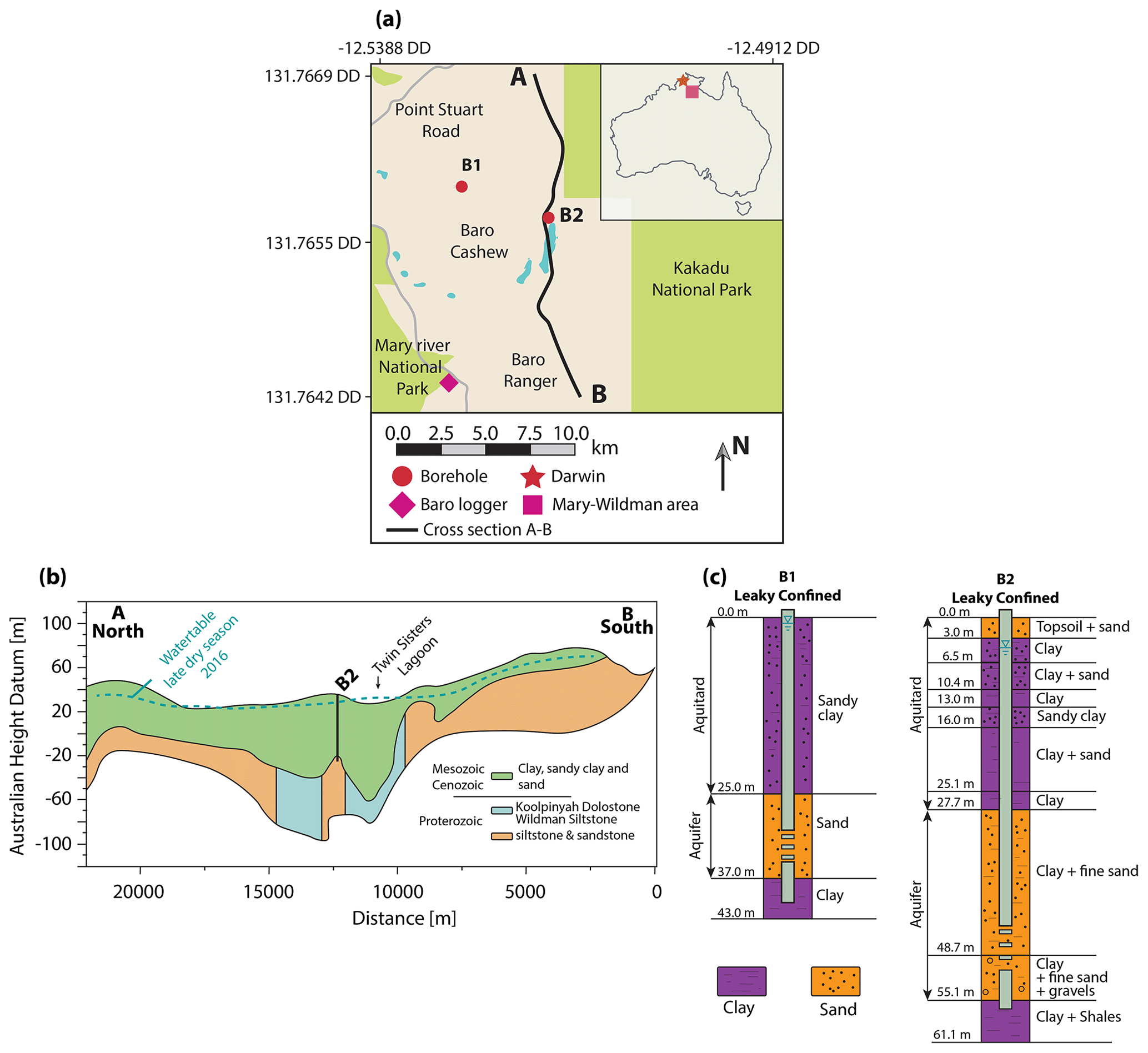
The study area is bounded by Mary River National Park in the west and by Kakadu National Park in the east. The intervening area has been of interest for irrigated agricultural development since the 1980s. The area features a subequatorial climate, with the dry season occurring between May and September and the wet season occurring between October and April. The highest annual mean air temperatures are recorded between October and December at around 35 ∘C and the lowest in July at around 16 ∘C (Tickell, 2017).
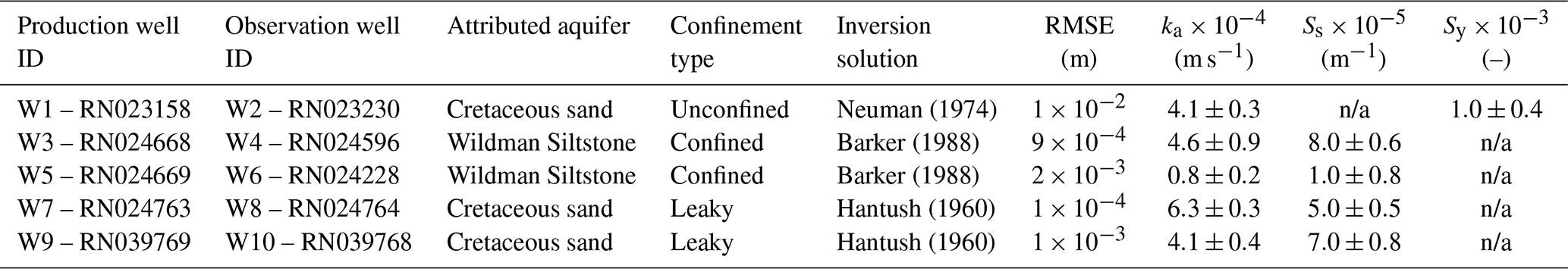
Two main hydrostratigraphic units are present as layers in the study area: (1) Mesozoic or Cenozoic sediments underlain by (2) the Proterozoic Koolpinyah Dolostone, in addition to siltstones and sandstones (Fig. 2a) (Tickell, 2017). Groundwater and mineral exploration wells are the main source of geological information as outcrops are rare. Mesozoic or Cenozoic sediments consist of unconsolidated to poorly consolidated sands, clayey sands, and clays. Lithological logs indicate that this unit is laterally extensive across the study area (Tickell, 2017). A leaky sandy clay aquitard partially confines a second semi-confined sand aquifer (B1 and B2 in Fig. 2c). This aquifer is sufficiently permeable to allow recharge to the semi-confined sand aquifer, as observed by increases in the groundwater level during each wet season. The Proterozoic strata consist primarily of the Koolpinyah Dolostone and the Wildman Siltstone. The hydrological behavior of this unit is conceptually a fractured aquifer (Tickell, 2017). Constant-rate discharge pumping tests indicate that the hydraulic conductivity of the Mesozoic or Cenozoic strata ranges from to m s−1 (Appendix B).
Groundwater monitoring datasets from two boreholes (B1 and B2) were analyzed in this work (Fig. 2b and Table 1). Note that the original nomenclature from the Australian Northern Territory (NT) was modified (Table 1). The lithological logs indicate that the boreholes are screened in the upper strata (Fig. 2c). In general, the upper two-thirds of the profile are clays and sandy clays that confine the underlying aquifer. The lower third often consists of sands, clayey sands, and gravels. Sands are mostly present as fine-grained quartz with limited occurrences of coarse sands to pebbles.
Table 1Groundwater well construction information: reference datum Geocentric Datum Of Australia (GDA) 1994. DD stands for decimal degrees.
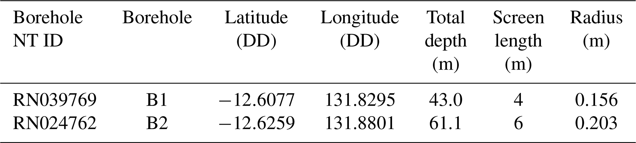
Well water levels were monitored hourly between June 2016 and September 2019 in each borehole using InSitu Level TROLL 400 data loggers (InSitu Inc., USA), and the sensor's sampling frequency was set to one sample per hour. The measured pressure heads were converted to hydraulic head values by referencing the dips of depth to water level manually to the surveyed top of casing elevations. Concurrently, barometric pressure was recorded from September 2016 to October 2017 using an InSitu BaroTROLL 500 data logger (InSitu Inc., USA), and the sensor's sampling frequency was set to one sample per hour.
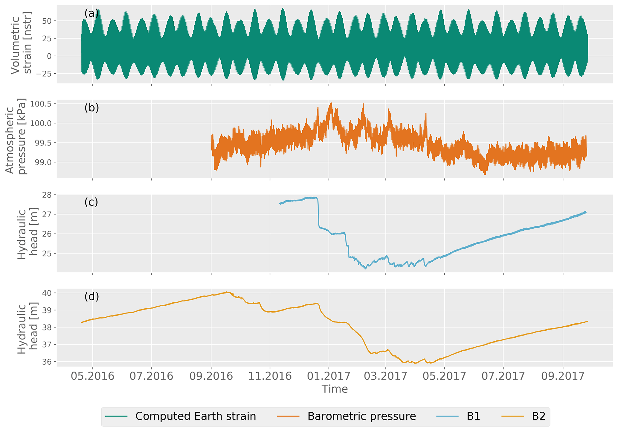
Figure 3Time series of (a) computed Earth tide strain in the nanostrain (nstr), (b) measurements of barometric pressure, and hydraulic head time series measured in boreholes B1 (c) and B2 (d).
3.2 Extraction of tidal responses
Earth tide strains, barometric pressure, and hydraulic heads in wells B1 and B2 are shown in Fig. 3. Outliers were identified using Pearson's rule, i.e., values that deviate more than 3 times from the median absolute deviation (MAD) (Pham-Gia and Hung, 2001) and are removed from the data (Figs. 1b and A1). Note that the overall head varies by about 2 m, reflecting the wet and dry seasons that are typical for tropical Australia. Earth tide strains were calculated using PyGTide (Rau, 2018), which is based on the widely used ETERNA PREDICT software (Wenzel, 1996) (Fig. 1c). To ensure that ocean tides have a negligible influence on the strain, the ocean tidal effect was computed using the Ocean Loading Model for Permanent and Persistent (OLMPP) method developed by H. G. Scherneck at the Onsala Space Observatory in 2023 at the study site located at latitude −12.607700 DD and longitude 131.829500 DD. For the M2 Earth tides, the amplitude is 21 times higher than that of the ocean loading, while for the S2 Earth tides, the amplitude is 37 times higher.
Harmonic tidal components of the dominant tidal components M2 (1.93 cpd) and S2 (2.0 cpd) (Merritt, 2004; McMillan et al., 2019) were extracted from all time series and locations following the methods outlined in Schweizer et al. (2021) and Rau et al. (2020).
-
The measured well water levels, barometric measurements, and computed Earth tidal strain were detrended using a moving linear regression filter with a 3 d window (Fig. 1d), and the results are shown in Fig. A2.
-
Amplitudes and phases of 10 tidal harmonic constituents were jointly estimated using harmonic least squares (HALS) (Fig. 1e). HALS was applied to the entire duration of the time series.
-
From HALS, amplitudes and phases of the M2 tidal components were obtained for Earth tidal strains and hydraulic heads. As the tidal component S2 encompasses both Earth tidal forces and atmospheric loading effects, the amplitudes and phases of the S2 tidal component were determined for Earth tide strains, hydraulic heads, and barometric pressure (Fig. 4b) as well as for hydraulic heads (Fig. 4c and d).
-
Complete disentanglement of the groundwater response to Earth and atmospheric tide influences was done for S2 following the method established by Rau et al. (2020) (Fig. 1f). This allows us to separate the effects of Earth tides and atmospheric tides for the S2 constituent.
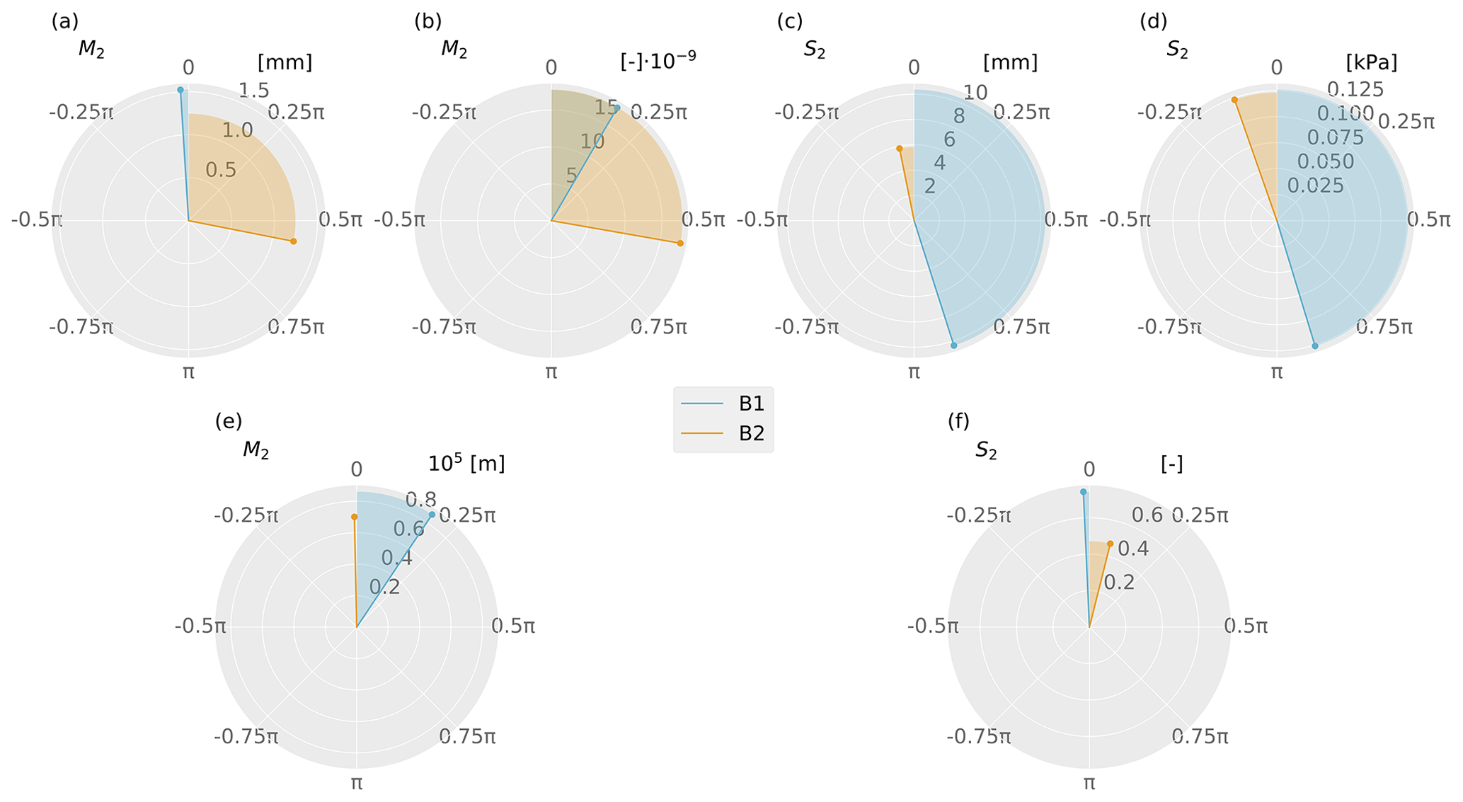
Figure 4Polar plots showing the M2 and S2 harmonics estimated from hydraulic heads in response to Earth and atmospheric tides for boreholes B1 and B2. (a) M2 constituent at measured well water levels. (b) M2 constituent in Earth tide strain data calculated at well locations. (c) S2 constituent at well water levels. (d) S2 constituent in Earth tide strain data calculated at well locations. (e) Amplitude and phase shift of the M2 constituent: Eqs. (16) and (17). (f) Amplitude ratio and phase shift of the S2 constituent: Eqs. (18) and (19).
The resulting amplitude of the hydraulic head (abbreviated as GW for groundwater) AGW can be divided by the Earth tide strain amplitude (abbreviated as ETP for Earth tides) AETP to obtain the amplitude ratio (Fig. 4e):
The phase shift can be obtained as the difference between the obtained phase of the hydraulic head measurements ϕGW and the computed Earth tide strain prediction ϕETP as
The resulting and for the hydraulic head and areal Earth tide strain for boreholes B1 and B2 are presented in Fig. 4e and Table A1.
Analogously, the ratio between the resulting amplitude of HALS of the hydraulic head AGW can be divided by the measured (time series) barometric pressure (abbreviated as ATP for atmospheric tides) AATP to obtain the amplitude ratio:
The phase shift can be obtained as the difference between the obtained phase of the hydraulic head measurements ϕGW and the measured barometric pressure ϕATP as
The resulting and for the hydraulic head and areal Earth tide strain for boreholes B1 and B2 are presented in Fig. 4f and Table A2.
3.3 Estimation of subsurface properties
To estimate subsurface parameters from the groundwater response to Earth tides, the analytical solution by Wang et al. (2018) was fitted to the M2 harmonic component extracted from field data. This analytical solution describes the well water level fluctuations, , caused by the harmonic compression of the subsurface from Earth tides (abbreviated as ET).
The reduction in the amplitude of a harmonic signal is described by the ratio between the far-field pressure generated by Earth tide strain and the fluid level in the borehole and is known as the amplitude ratio (Hsieh et al., 1987):
where ϵ is the unitless areal strain. The time lag between the far-field pressure and the fluid level in the borehole is known as the phase shift (Hsieh et al., 1987):
In theory, the obtained amplitude and phase shift from field measurements (Eqs. 16 and 17) should be the same as those obtained using the analytical solution (Eqs. 20 and 21). Since the observed amplitude, , and phase shift, , are measurable in the field, they can be used to fit parameters of the analytical solution of Wang et al. (2018) with a nonlinear solver to find roots (Fig. 1g). To do so, the following objective function has to be minimized:
Since phase shifts can be orders of magnitude greater than the amplitude ratio, OFET is normalized to prevent one term from dominating the solution. Assuming that the borehole construction parameters are known (Ha, Hl, rc, and rw), three parameters can be estimated, i.e., hydraulic conductivity of the aquifer (ka), vertical hydraulic conductivity of the leaky layer (kl), and specific storage at constant strain (Sϵ). Once Sϵ is obtained, effective porosity can be computed if the material is unconsolidated using (Cheng, 2016; Verruijt, 2013; Wang, 2017)
where Kf is the bulk modulus of the fluid ( Pa for freshwater).
In analogy to Earth tides, the field measurements of barometric pressure and well water levels in the field should match those obtained by analytical methods. Thus, the obtained amplitude ratio, , and the phase shift, , in the field (computed later with Eqs. 18 and 19, respectively) can be used to estimate subsurface parameters by iterative nonlinear numerical methods (Fig. 1h). The function to minimize is
The nonlinear search allows for the iterative fitting of four parameters: hydraulic conductivity of the aquifer (ka), vertical hydraulic conductivity of the leaky layer (kl), bulk modulus (K), and specific storage at constant strain (Sϵ). Additionally, specific storage at constant stress (Sσ) can be estimated using Eq. (12).
Once Sϵ is estimated, porosity can be computed with Eq. (23). Specific storage, S, can be obtained if the barometric efficiency ( in this study) is known (Cheng, 2016; Verruijt, 2013; Wang, 2017):
Then, the shear modulus can also be estimated as (Cheng, 2016; Verruijt, 2013; Wang, 2017)
By solving Eq. (22), aquifer hydraulic conductivity ka, specific storage at constant strain Sϵ, and vertical hydraulic conductivity of the aquitard kl can be estimated. Equation (24) allows estimation of aquifer hydraulic conductivity ka, specific storage at constant strain Sσ, vertical hydraulic conductivity of the aquitard kl, and bulk modulus K. Once specific storage at constant strain is quantified, porosity n can be estimated with Eq. (23). Specific storage S can be obtained with Eq. (25), and shear modulus G can be estimated with Eq. (26). Equations (22) and (24) can be solved using nonlinear iteration (Fig. 1g and h).
The nonlinear inversion was performed in two steps to help the iterative method converge to a global minimum instead of a local one. Firstly, the solution space of the objective function was divided into intervals within feasible ranges of subsurface properties, creating a feasible objective space and thus bounding the initial conditions for the least-squares algorithm. Secondly, 1000 randomly generated values following a log-normal distribution were fed as initial conditions to the least-squares algorithm. The array of parameters that converges to the best fit among them was considered to be the global minimum of the nonlinear search (Aster et al., 2018).
3.4 Hydraulic and geomechanical properties
Values from Earth tide analysis and atmospheric tide analysis are presented in Tables 2 and 3. Further, the estimated aquifer hydraulic conductivity, specific storage at constant strain, and aquitard vertical hydraulic conductivity for boreholes B1 and B2 are shown in Fig. 5.
Table 2Estimated subsurface parameters from Earth tide analysis.
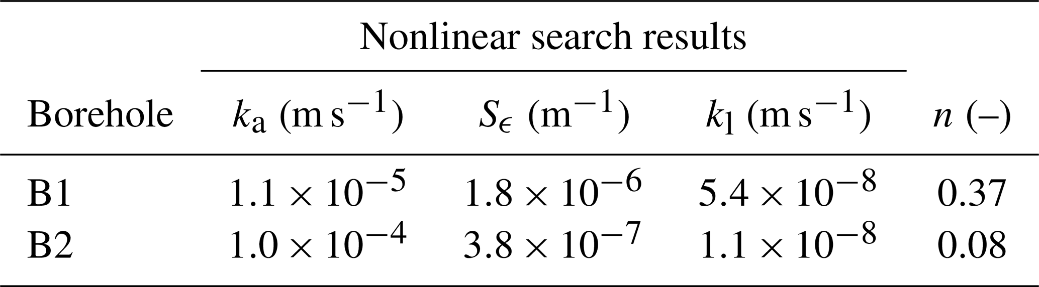
Table 3Estimated subsurface parameters from atmospheric tide analysis.
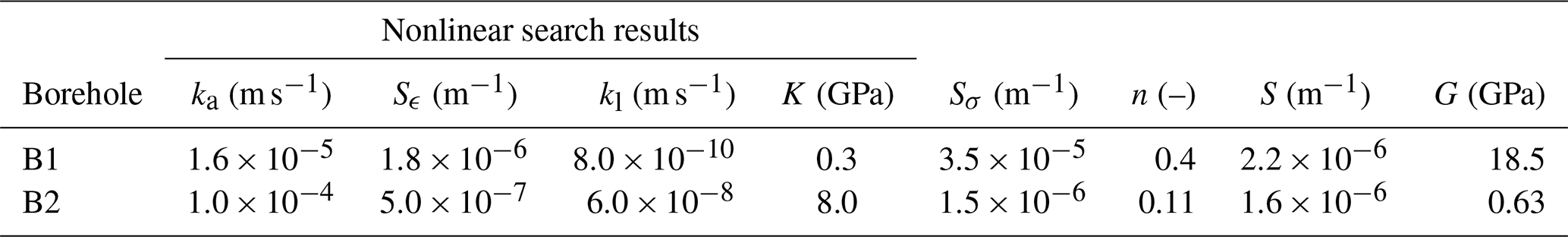
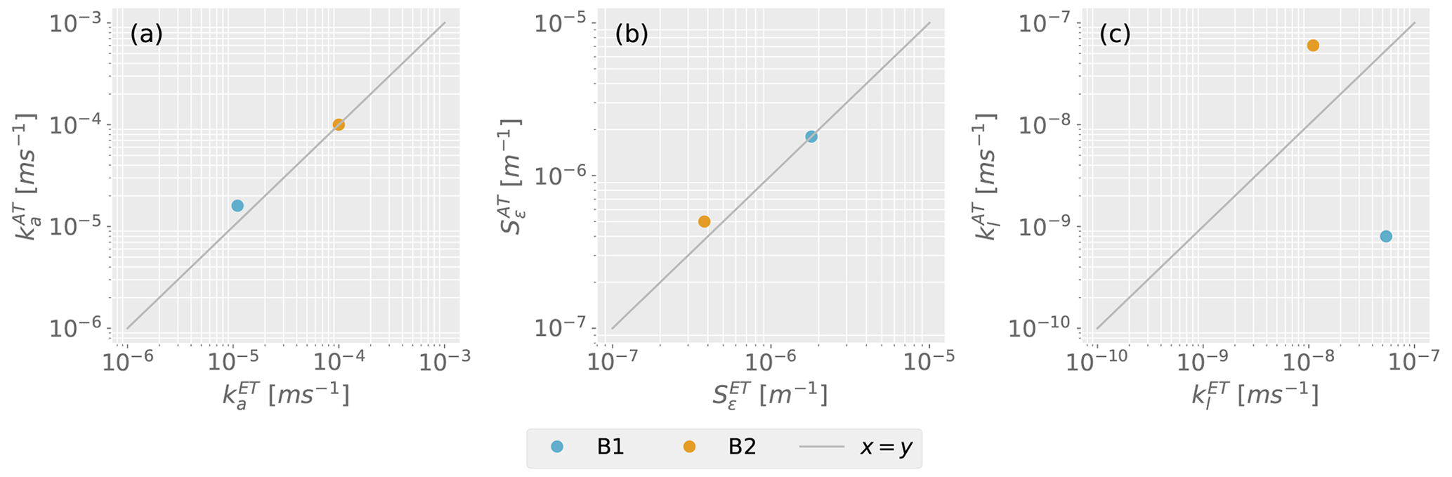
Figure 5Comparison of the subsurface parameters estimated independently using the well water level response to Earth tides and atmospheric tides: (a) hydraulic conductivity of the aquifer, (b) specific storage at constant strain, and (c) vertical hydraulic conductivity of the aquitard.
The basic assumption of undrained conditions applies to the analytical solutions by Wang et al. (2018) and this study (Eq. 9). To assess whether this condition is fulfilled, both Earth and atmospheric tide analyses were assessed separately.
-
For Earth tide analysis, Bastias et al. (2022) numerically computed the level of drainage over depth for different arrays of subsurface properties. Despite the estimated kl being outside the range presented by Bastias et al. (2022), it can be extrapolated. At borehole B1, the aquifer is within undrained conditions. At borehole B2, it is within the transition zone between drained and undrained conditions.
-
For atmospheric tide analysis, Wang (2017) defined the depth of undrained conditions as
where c is the consolidation coefficient. For boreholes B1 and B2, undrained conditions are found at depths greater than 2.3 and 40.6 m, respectively, under atmospheric tide loading.
Consequently, for the estimated parameters in this study, B2 borders drained conditions, and the generated confined pore pressure by tidal forcing is being diminished. This may influence the estimated properties.
The aquifer hydraulic conductivity estimated with PSC complies with previous values of poorly consolidated sands and gravel aquifers in the literature ( m s−1) (Freeze and Cherry, 1979; Tickell, 2017) (Fig. 5a, Tables 2 and 3). Note that the estimated value of ka is lower compared to the pumping tests at the study site (Table B1). Bastias et al. (2022) studied the area of influence of PSC and concluded that PSC is a small-scale characterization technique where parameters are estimated in the vicinity of the well screen. This might explain the difference between values presented in this study and the ones obtained with pumping tests (Appendix B), as parameters estimated with small-scale methods will tend to give much lower values than those obtained from a full-well or packer pumping test, because small-scale analyses may miss the most permeable intervals that make the greatest contribution to the transmissivity (Maliva, 2016). This idea is supported by previous studies that reported differences of several orders of magnitude between traditional hydraulic characterization methods and PSC (Allègre et al., 2016; Zhang et al., 2019; Valois et al., 2022; Qi et al., 2023). The difference was attributed to issues such as the borehole skin effect (Zhang et al., 2019; Valois et al., 2022) and differing model assumptions (Qi et al., 2023). Furthermore, Zhang et al. (2021) showed good agreement between hydraulic parameters of a consolidated subsurface system derived using PSC and laboratory measurements. This supports our observation that PSC results are representative of a smaller sample volume close to the well screen. However, determining the extent of the area around the well screen affected by flow from tidal forces is outside the scope of this work and requires further investigation. Additionally, reconciling the properties derived from both active and passive approaches will require more research.
The estimated values of specific storage at constant strain for borehole B1 are within the previously reported values in the literature for sand aquifers, m−1 (Freeze and Cherry, 1979) (Fig. 5b). Porosity, computed with Eq. (23), is also within the reported range: (Freeze and Cherry, 1979). Conversely, borehole B2 shows that values of specific storage at constant strain and porosity are below the expected range (Tables 2 and 3). There are several potential causes of this, such as the presence of flow paths that create undrained conditions, leading to a reduction in the generated confined pore pressure and exposing the limitations of passive methods for this borehole (Bastias et al., 2022; Wang, 2017; Cheng, 2016). Furthermore, the degree of aquifer consolidation is limited, and the length of the well screen is not representative of the full depth of the aquifer. These factors were not explored in this study and should be the focus of future numerical investigations to better understand their effects on the results.
The estimated aquifer bulk modulus values (Table 3) were consistent with literature values for sands and gravels, typically between and 3×101 GPa (Das and Das, 2008; Look, 2007). The estimated values of specific storage were consistent with the pumping tests performed at the study site (assuming low spacial variability of the hydrogeomechanical properties, Fig. B1). Once specific storage is estimated, shear modulus can be estimated with Eq. (26). We note that these values are consistent with expectations reported in the literature for similar lithological settings, e.g., typically between and 9×10³ GPa (Das and Das, 2008; Look, 2007).
Compared to the previous analytical solution presented by Rojstaczer and Riley (1990), which describes flow to wells due to barometric loading, the derived analytical solution in this study simplifies the pore pressure wave generated in the vadose zone by assuming that only small vertical flow occurs in the confined layer. Moreover, the solution of Rojstaczer and Riley (1990) requires knowledge of vadose zone properties that are difficult to determine. Furthermore, the continuity equation is solved in terms of the mean stress equation, allowing for the estimation of mechanical parameters such as bulk modulus and specific storage at constant stress. As shown in our work, this extends the current range of parameters that can be estimated passively (McMillan et al., 2019).
While we present a new analytical solution, we are unable to compare or validate geomechanical results due to a lack of independent measurements. Additionally, the literature comparing subsurface properties using PSC from different methods is sparse and contains somewhat conflicting conclusions (Allègre et al., 2016; Zhang et al., 2019; Valois et al., 2022; Qi et al., 2023; Zhang et al., 2021). This is likely due to the fact that subsurface investigations often focus on determining hydraulic properties such as hydraulic conductivity and specific storage, which are critical for understanding subsurface fluid flow. Obtaining geomechanical information such as bulk modulus, shear modulus, and stress state can be challenging and may require additional investigation techniques. However, Rau et al. (2022) noted that in the field stress conditions, stress anisotropy, and scale differences complicate comparisons with laboratory methods. We believe that systematic investigations in different archetypes of formations, including the use of borehole geophysical investigation techniques and careful laboratory testing of material samples, could help to clarify scale and heterogeneity influences, reconcile the different theories, and provide further confidence in values derived from PSC.
We have introduced a novel analytical solution based on the mean stress flow equation for modeling flow to wells induced by atmospheric loading. We integrate this mean stress solution into a comprehensive workflow for estimating subsurface hydraulic and geomechanical properties using the groundwater response to Earth and atmospheric tides, applied this to a standard groundwater monitoring dataset from the Northern Territory (Australia), and discussed the results with hydraulic properties from pumping tests and geomechanical literature values for similar lithological settings. Our new solution allows estimation of hydraulic conductivity of the aquifer, vertical hydraulic conductivity of the aquitard, porosity, specific storage at a constant strain, and specific storage at a constant stress and bulk modulus. The advantages are estimations of additional subsurface properties without the need for knowledge of vadose zone properties.
We compared the hydraulic properties estimated independently using the groundwater response to Earth tides and atmospheric pressure. After constraining the solution space based on feasible values derived from the lithology information obtained from the well logs, 1000 randomly generated values were employed as initial conditions for the least-squares algorithm. These values were generated according to a log-normal distribution. The purpose was to obtain an array of parameters that would converge to the best fit. The estimated values of aquifer hydraulic conductivity with Earth tidal analysis were and m s−1 for boreholes B1 and B2, respectively. Meanwhile, with the mean stress solution, the estimated values of aquifer hydraulic conductivity were and m s−1 for boreholes B1 and B2, respectively. These estimated values were lower than those estimated using pumping tests for the region between Mary River National Park and Kakadu National Park (ranging from to m s−1). This difference is consistent with the literature and supports the idea that PSC is a small-scale characterization method.
The estimated specific storage at constant strain for borehole B2 was and m−1 with Earth tidal analysis and the mean stress equation, respectively. This indicates that the response near borehole B2 is drained since the estimated values are lower than the reported bounds in the literature. Consequently, the drained conditions reduce the confined pore pressure generated by tides. The estimated values of aquitard vertical hydraulic conductivity differed from the pumping tests by orders of magnitude but suggest that the aquifer in both boreholes is semi-confined with small leakage.
The bulk and shear moduli aligned with literature values for the formation type, confirming that PSC has the potential to enhance field investigations. However, for PSC to be applied successfully, it is necessary for the basic physical assumptions underlying the analytical solutions to be valid. This can be challenging to determine in situations such as confined and undrained hydraulic conditions or an unconsolidated system where the Biot coefficient is unknown. As a result, PSC can only be applied in hydrogeological settings that adhere to the theoretical framework.
Compared to established methods like hydraulic testing, using PSC requires a better understanding of hydraulic and hydrogeomechanical theory as well as signal processing. However, PSC is less costly and effort-intensive because it only requires monitoring datasets that typically meet standard practice criteria. The literature reflects confusion about the suitability of theory and a lack of geomechanical testing alongside hydraulic testing, making it challenging to validate poroelastic properties. Systematic investigations involving a range of archetypal formations with a combination of hydraulic, geophysical, and geotechnical field and laboratory tests are needed to validate PSC. This would help compare properties from rigid and elastic formations, reconcile theories, and support groundwater and geotechnical investigations.
Analytical solutions assume simplified systems that often fail to comply with complex geologic formations. This discrepancy can result in significant errors when the assumptions of analytical solutions are violated. To assess the impact of such assumptions, two approaches can be considered. Firstly, numerical models can be employed to elucidate potential discrepancies between analytical and numerical solutions when the fundamental assumptions underlying analytical solutions are violated. Secondly, more intricate analytical or semi-analytical solutions can be developed that incorporate the mechanical effects of undrained conditions and/or consolidated systems.
The hydraulic head measurements in boreholes B1 and B2 are shown in Fig. A1. Outliers were detected and eliminated with the procedure described in Sect. 3.2.
Computed areal Earth tide strain, measured barometric pressure, and hydraulic heads of boreholes B1 and B2 were detrended using a moving median filter with a 3 d window (Sect. 3.2 and Fig. A2).
Harmonic constituents were obtained by applying harmonic least squares (HALS). Results of amplitude and phase shift to the M2 signal are shown in Table A1. Analogously, the amplitude and the phase shift to the S2 signal are shown in Table A2.
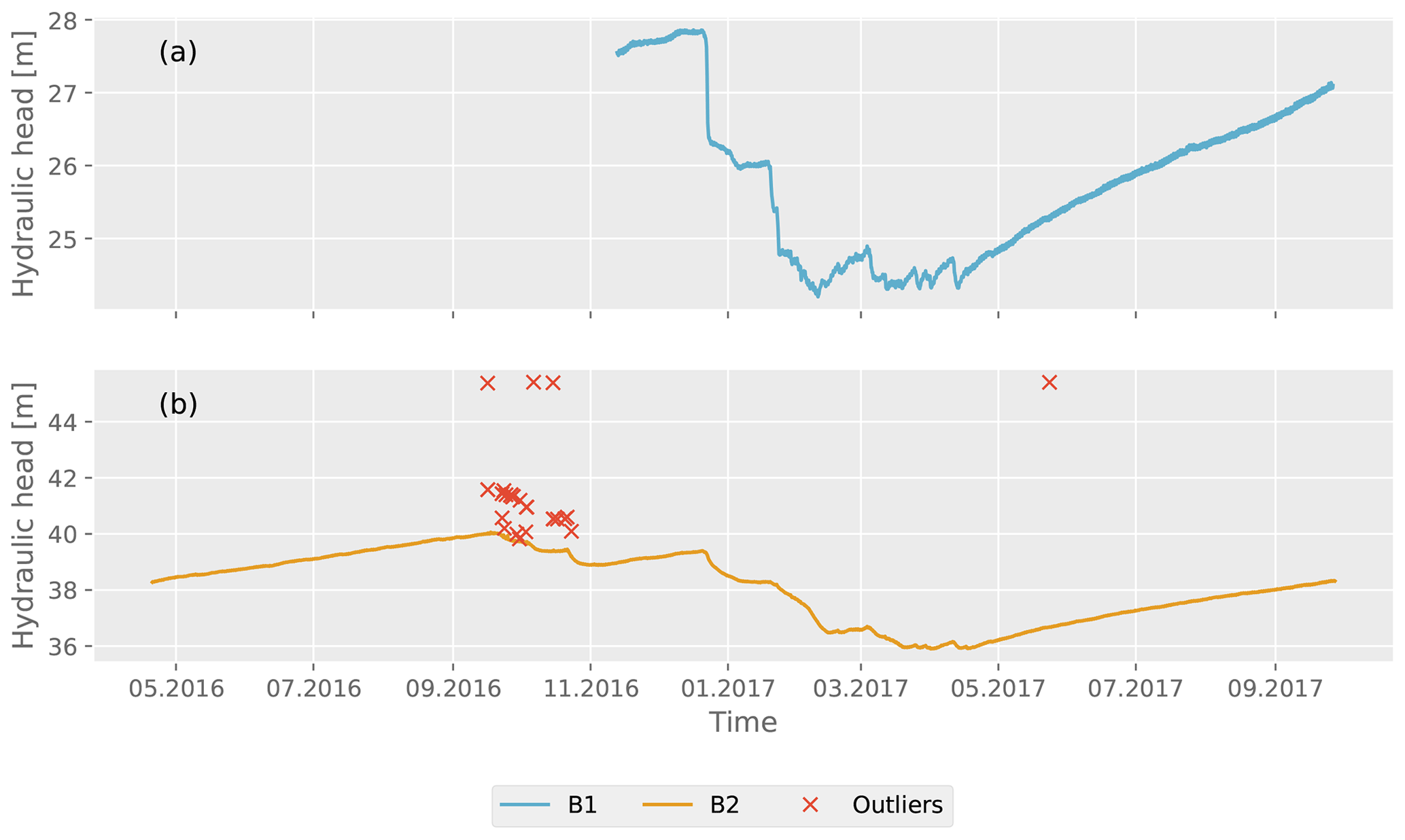
Table A1Amplitude ratio and phase shift obtained with HALS for the M2 constituent.
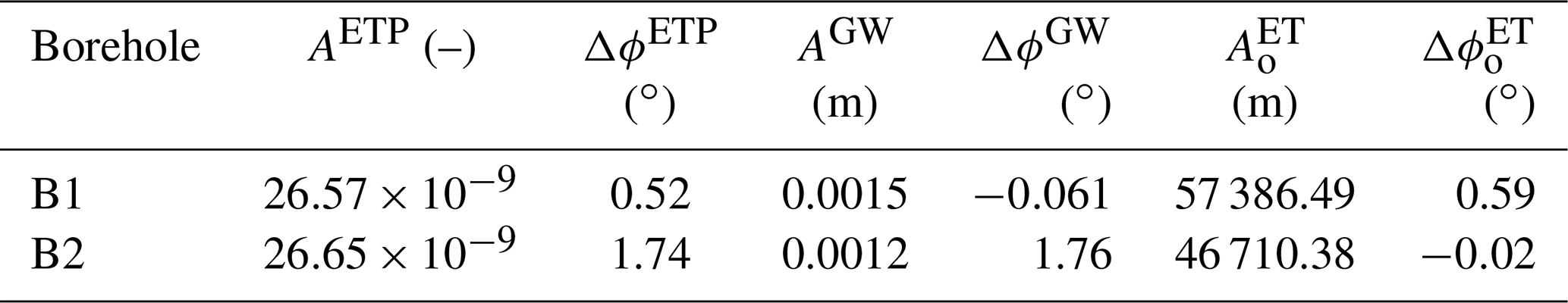
Table A2Amplitude ratio and phase shift obtained with HALS for the S2 constituent.
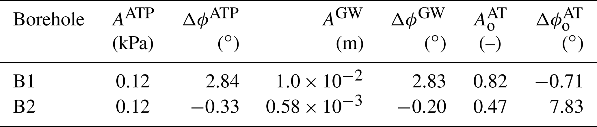
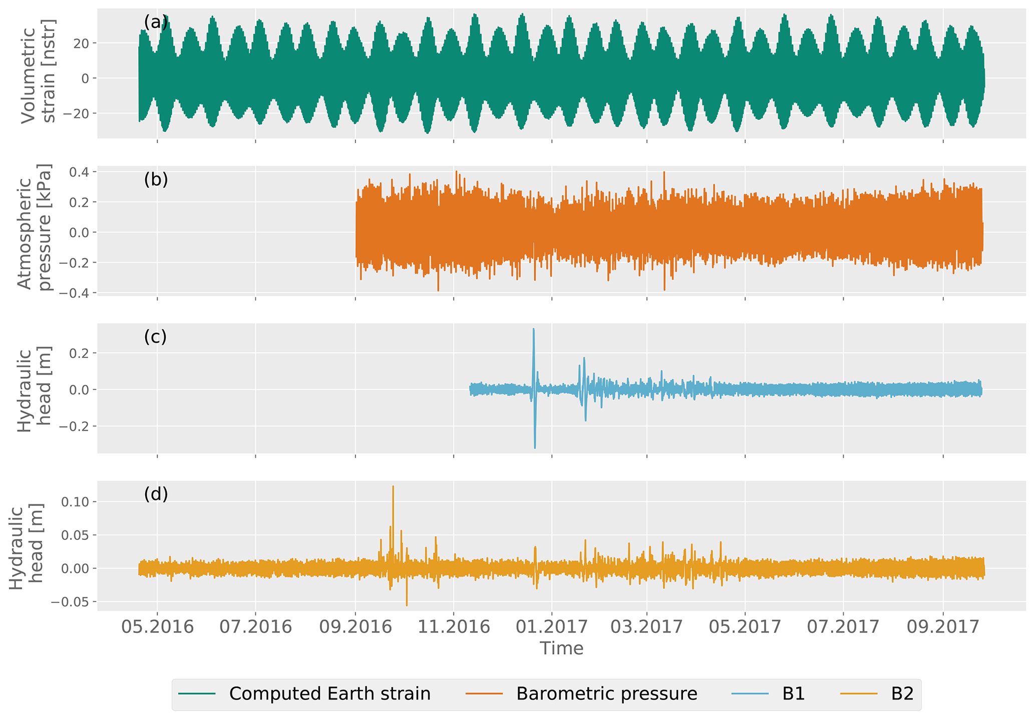
Figure A2The corresponding detrended time series showing only components with frequencies of up to 3 cpd. (a) Computed Earth strain, (b) measured atmospheric pressure and hydraulic head, (c) B1, and (d) B2.
Time–drawdown data from five two-well pumping tests in the Mary–Wildman river area were reinterpreted using appropriate drawdown solutions and a two-step process (see Table B1 and W1 to W10 in Fig. B1a) (Turnadge et al., 2018). The time–drawdown data were used to identify appropriate pumping test analysis solutions. These included the solutions of Barker (1988) for fractured rock flow under confined conditions, Hantush (1960) for leaky conditions, and Neuman (1974) for unconfined conditions.
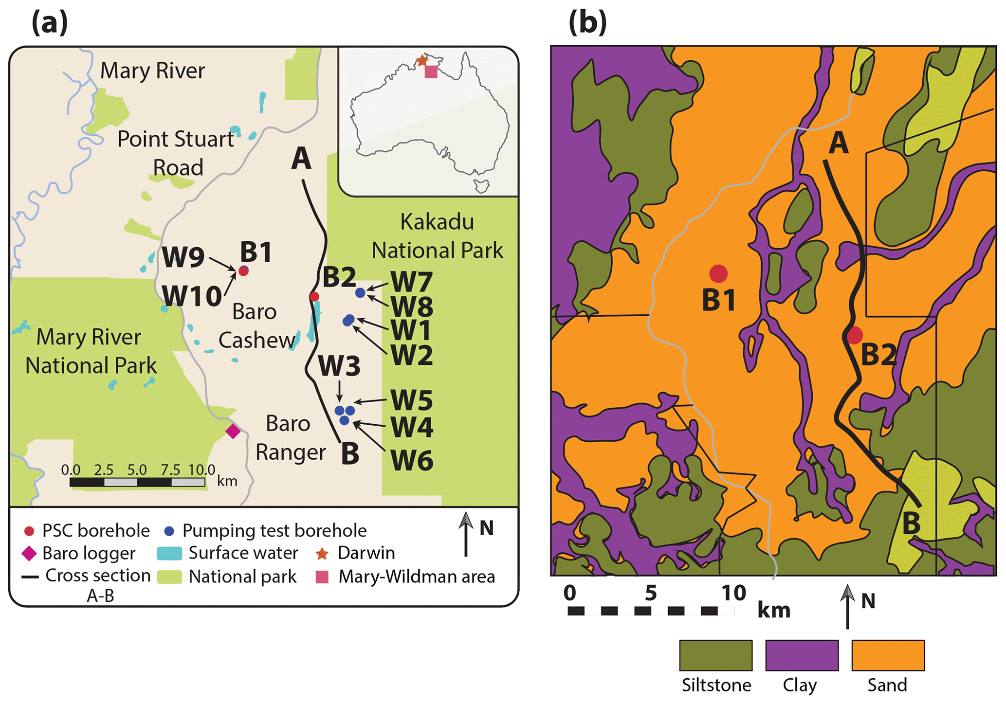
Figure B1Map of the study site. Panel (a) shows the PSC boreholes, barometric sensors, and locations of the wells where pumping tests were performed (wells W1 to W10). Panel (b) shows the surface geology of the Mesozoic and Cenozoic strata (modified from NT Geological Survey digital data: Tickell, 2017).
Table B1Details of five historical two-well pumping tests undertaken in the Mary–Wildman river area, including aquifer types interpreted from time–drawdown responses and forward solutions used to estimate aquifer hydraulic properties via model inversion. Hydraulic property values are displayed with the root mean square error of the optimized least-squares solution. For each estimated parameter, the optimal value derived from least-squares estimation is provided together with the approximate 95 % confidence interval. The abbreviation n/a stands for “not applicable”.
Python files to read and visualize the data and key figures generated for this study are available at a Zenodo repository (https://doi.org/10.5281/zenodo.8200689, Bastías Espejo, 2023) with an MIT license.
Hydraulic head and barometric pressure measurements are available at a Zenodo repository (https://doi.org/10.5281/zenodo.8200689, Bastías Espejo, 2023) with an MIT license.
JMBE analyzed the datasets, created the figures, and wrote the first manuscript draft. CT and RC provided the datasets and reviewed the work. CT analyzed the pumping tests. PB reviewed the manuscript and provided conceptual suggestions. GCR obtained the funding, supervised JMBE, and actively contributed to all aspects of this work.
The contact author has declared that none of the authors has any competing interests.
Publisher's note: Copernicus Publications remains neutral with regard to jurisdictional claims in published maps and institutional affiliations.
The authors would like to thank the following individuals, who conducted fieldwork to collect the datasets used here: Steven Tickell, Ursula Zaar, Gary Willis, Steve Dwyer, Emma Jackson, Ian Bate, Stanley Smith, Alec Deslandes, Karen Barry, Simone Gelsinari, and Julia Knollmann.
This research was supported by the Deutsche Forschungsgemeinschaft (grant no. 424795466).
The article processing charges for this open-access publication were covered by the Karlsruhe Institute of Technology (KIT).
This paper was edited by Nadia Ursino and reviewed by two anonymous referees.
Acworth, R. I., Halloran, L. J., Rau, G. C., Cuthbert, M. O., and Bernardi, T. L.: An objective frequency domain method for quantifying confined aquifer compressible storage using Earth and atmospheric tides, Geophys. Res. Lett., 43, 11–671, 2016. a
Acworth, R. I., Rau, G. C., Halloran, L. J., and Timms, W. A.: Vertical groundwater storage properties and changes in confinement determined using hydraulic head response to atmospheric tides, Water Resour. Res., 53, 2983–2997, 2017. a
Allègre, V., Brodsky, E. E., Xue, L., Nale, S. M., Parker, B. L., and Cherry, J. A.: Using earth-tide induced water pressure changes to measure in situ permeability: A comparison with long-term pumping tests, Water Resour. Res., 52, 3113–3126, https://doi.org/10.1002/2015WR017346, 2016. a, b
Arditty, P. C., Ramey, H. J., and Nur, A. M.: Response of a closed well-reservoir system to stress induced by earth tides, in: Spe annual fall technical conference and exhibition, OnePetro, https://doi.org/10.2118/7484-MS, 1978. a
Aster, R. C., Borchers, B., and Thurber, C. H.: Parameter estimation and inverse problems, Elsevier, https://doi.org/10.1016/C2009-0-61134-X, 2018. a
Barker, J.: A generalized radial flow model for hydraulic tests in fractured rock, Water Resour. Res., 24, 1796–1804, 1988. a, b, c
Bastías Espejo, J.: josebastiase/Mean-Stress: Mean-Stress_v1.0, Zenodo [data set] and [code], https://doi.org/10.5281/zenodo.8200689, 2023. a, b
Bastias, J., Rau, G. C., and Blum, P.: Groundwater responses to Earth tides: Evaluation of analytical solutions using numerical simulation, J. Geophys. Res.-Sol. Ea., 127, e2022JB024771, https://doi.org/10.1029/2022JB024771, 2022. a, b, c, d
Biot, M. A.: General theory of three-dimensional consolidation, J. Appl. Phys., 12, 155–164, 1941. a
Bodvarsson, G.: Confined fluids as strain meters, J. Geophys. Res., 75, 2711–2718, 1970. a
Bredehoeft, J. D.: Response of well-aquifer systems to Earth tides, J. Geophys. Res., 72, 3075–3087, 1967. a
Cheng, A. H.-D.: Poroelasticity, in: vol. 27, Springer, https://doi.org/10.1007/978-3-319-25202-5, 2016. a, b, c, d, e, f, g, h, i, j, k, l, m
Cooper Jr., H. H., Bredehoeft, J. D., Papadopulos, I. S., and Bennett, R. R.: The response of well-aquifer systems to seismic waves, J. Geophys. Res., 70, 3915–3926, 1965. a, b
Cutillo, P. A. and Bredehoeft, J. D.: Estimating aquifer properties from the water level response to earth tides, Groundwater, 49, 600–610, 2011. a, b
Das, B. M. and Das, B.: Advanced soil mechanics, in: vol. 270, Taylor & Francis New York, https://doi.org/10.1201/9781351215183 , 2008. a, b
Doan, M.-L., Brodsky, E. E., Prioul, R., and Signer, C.: Tidal analysis of borehole pressure – A tutorial, University of California, Santa Cruz, https://websites.pmc.ucsc.edu/~brodsky/reprints/tidal_tutorial_SDR.pdf (last access: 11 September 2023), 2006. a
Domenico, P. A. and Schwartz, F. W.: Physical and chemical hydrogeology, John Wiley & Sons, https://doi.org/10.1017/S0016756800019890, 1997. a
Freeze, R. A. and Cherry, J. A.: Groundwater, Prentice Hall, Inc., Upper Saddle River, http://hydrogeologistswithoutborders.org/wordpress/1979-toc/ (last access: 11 September 2023), 1979. a, b, c, d
Gao, X., Sato, K., and Horne, R. N.: General solution for tidal behavior in confined and semiconfined aquifers considering skin and wellbore storage effects, Water Resour. Res., 56, e2020WR027195, https://doi.org/10.1029/2020WR027195, 2020. a
Guo, H., Brodsky, E., Goebel, T., and Cladouhos, T.: Measuring Fault Zone and Host Rock Hydraulic Properties Using Tidal Responses, Geophys. Res. Lett., 48, e2021GL093986, https://doi.org/10.1029/2021GL093986, 2021. a
Hantush, M. S.: Modification of the theory of leaky aquifers, J. Geophys. Res., 65, 3713–3725, 1960. a, b, c
Hsieh, P. A., Bredehoeft, J. D., and Farr, J. M.: Determination of aquifer transmissivity from Earth tide analysis, Water Resour. Res., 23, 1824–1832, 1987. a, b, c, d, e
Lai, G., Ge, H., and Wang, W.: Transfer functions of the well-aquifer systems response to atmospheric loading and Earth tide from low to high-frequency band, J. Geophys. Res.-Sol. Ea., 118, 1904–1924, 2013. a
Lai, G., Ge, H., Xue, L., Brodsky, E. E., Huang, F., and Wang, W.: Tidal response variation and recovery following the Wenchuan earthquake from water level data of multiple wells in the nearfield, Tectonophysics, 619, 115–122, 2014. a
Le Borgne, T., Bour, O., De Dreuzy, J., Davy, P., and Touchard, F.: Equivalent mean flow models for fractured aquifers: Insights from a pumping tests scaling interpretation, Water Resour. Res., 40, W03512, https://doi.org/10.1029/2003WR002436, 2004. a
Liang, X., Wang, C.-Y., Ma, E., and Zhang, Y.-K.: Effects of Unsaturated Flow on Hydraulic Head Response to Earth Tides – An Analytical Model, Water Resour. Res., 58, e2021WR030337, https://doi.org/10.1029/2021WR030337, 2022. a
Look, B. G.: Handbook of geotechnical investigation and design tables, Taylor & Francis, ISBN 9781138452756, 2007. a, b
Maliva, R. G.: Aquifer characterization techniques, in: vol. 10, Springer, https://doi.org/10.1007/978-3-319-32137-0, 2016. a, b
McMillan, T. C., Rau, G. C., Timms, W. A., and Andersen, M. S.: Utilizing the impact of Earth and atmospheric tides on groundwater systems: A review reveals the future potential, Rev. Geophys., 57, 281–315, 2019. a, b, c, d, e, f, g, h, i
Meinzer, O. E.: Ground water in the United States, a summary of ground-water conditions and resources, utilization of water from wells and springs, methods of scientific investigation, and literature relating to the subject, Tech. rep., US G.P.O., http://pubs.er.usgs.gov/publication/wsp836D (last access: 11 September 2023), 1939. a
Merritt, M. L.: Estimating hydraulic properties of the Floridan aquifer system by analysis of earth-tide, ocean-tide, and barometric effects, Collier and Hendry Counties, Florida, 3, US Department of the Interior, US Geological Survey, https://doi.org/10.3133/wri034267, 2004. a, b, c, d
Neuman, S. P.: Effect of partial penetration on flow in unconfined aquifers considering delayed gravity response, Water Resour. Res., 10, 303–312, 1974. a, b
Pham-Gia, T. and Hung, T. L.: The mean and median absolute deviations, Math. Comput. Model., 34, 921–936, 2001. a
Qi, Z., Shi, Z., and Rasmussen, T. C.: Time- and frequency-domain determination of aquifer hydraulic properties using water-level responses to natural perturbations: A case study of the Rongchang Well, Chongqing, southwestern China, J. Hydrol., 617, 128820, https://doi.org/10.1016/j.jhydrol.2022.128820, 2023. a, b, c
Rahi, K. A. and Halihan, T.: Identifying aquifer type in fractured rock aquifers using harmonic analysis, Groundwater, 51, 76–82, 2013. a
Rau, G. C.: hydrogeoscience/pygtide: PyGTid, Zenodo [code], https://doi.org/10.5281/zenodo.1346260, 2018. a
Rau, G. C., Cuthbert, M. O., Acworth, R. I., and Blum, P.: Technical note: Disentangling the groundwater response to Earth and atmospheric tides to improve subsurface characterisation, Hydrol. Earth Syst. Sci., 24, 6033–6046, https://doi.org/10.5194/hess-24-6033-2020, 2020. a, b, c, d
Rau, G. C., McMillan, T. C., Andersen, M. S., and Timms, W. A.: In situ estimation of subsurface hydro-geomechanical properties using the groundwater response to semi-diurnal Earth and atmospheric tides, Hydrol. Earth Syst. Sci., 26, 4301–4321, https://doi.org/10.5194/hess-26-4301-2022, 2022. a, b, c
Robinson, E. S. and Bell, R. T.: Tides in confined well-aquifer systems, J. Geophys. Res., 76, 1857–1869, 1971. a
Roeloffs, E. A., Burford, S. S., Riley, F. S., and Records, A. W.: Hydrologic effects on water level changes associated with episodic fault creep near Parkfield, California, J. Geophys. Res., 94, 12387, https://doi.org/10.1029/jb094ib09p12387, 1989. a
Rojstaczer, S.: Determination of fluid flow properties from the response of water levels in wells to atmospheric loading, Water Resour. Res., 24, 1927–1938, 1988. a
Rojstaczer, S. and Riley, F. S.: Response of the water level in a well to earth tides and atmospheric loading under unconfined conditions, Water Resour. Res., 26, 1803–1817, 1990. a, b, c
Schweizer, D., Ried, V., Rau, G. C., Tuck, J. E., and Stoica, P.: Comparing Methods and Defining Practical Requirements for Extracting Harmonic Tidal Components from Groundwater Level Measurements, Math. Geosci., 53, 1147–1169, https://doi.org/10.1007/s11004-020-09915-9, 2021. a
Shi, Z. and Wang, G.: Aquifers switched from confined to semiconfined by earthquakes, Geophys. Res. Lett., 43, 11–166, 2016. a
Tickell, Z.: Water Resources of the Wildman River Area, Northern Territory Government, https://territorystories.nt.gov.au/10070/428586/0/53 (last access: 11 September 2023), 2017. a, b, c, d, e, f, g
Turnadge, C., Crosbie, R., Tickell, S., Zaar, U., Smith, S., Dawes, W., Davies, P., Harrington, G., and Taylor, A.: Hydrogeological characterisation of the Mary–Wildman rivers area, Northern Territory, https://publications.csiro.au/rpr/download?pid=csiro:EP185984&dsid=DS3 (last access: 11 September 2023), 2018. a
Valois, R., Rau, G. C., Vouillamoz, J.-M., and Derode, B.: Estimating hydraulic properties of the shallow subsurface using the groundwater response to Earth and atmospheric tides: a comparison with pumping tests, Water Resour. Res., 58, e2021WR031666, https://doi.org/10.1029/2021WR031666, 2022. a, b, c, d
Van der Kamp, G. and Gale, J.: Theory of earth tide and barometric effects in porous formations with compressible grains, Water Resour. Res., 19, 538–544, 1983. a
Verruijt, A.: Theory and problems of poroelasticity, Delft University of Technology, Delft, https://vulcanhammernet.files.wordpress.com/2017/01/poroelasticity2014.pdf (last access: 11 September 2023), 71 pp., 2013. a, b, c, d, e, f, g, h, i, j, k, l
Wang, H. F.: Theory of linear poroelasticity with applications to geomechanics and hydrogeology, Princeton University Press, https://doi.org/10.1515/9781400885688, 2017. a, b, c, d, e, f, g, h, i, j, k, l, m, n, o
Wang, C. Y., Doan, M. L., Xue, L., and Barbour, A. J.: Tidal response of groundwater in a leaky aquifer – Application to Oklahoma, Water Resour. Res., 54, 8019–8033, 2018. a, b, c, d, e
Wenzel, H.-G.: The nanoGal software: Earth tide data processing package: Eterna 3.3, Bulletin d'Informations des Marées Terrestres, 124, 9425–9439, 1996. a
Xue, L., Brodsky, E. E., Erskine, J., Fulton, P. M., and Carter, R.: A permeability and compliance contrast measured hydrogeologically on the San Andreas Fault, Geochem. Geophy. Geosy., 17, 858–871, 2016. a, b
Zhang, S., Shi, Z., and Wang, G.: Comparison of aquifer parameters inferred from water level changes induced by slug test, earth tide and earthquake – A case study in the three Gorges area, J. Hydrol., 579, 124169, https://doi.org/10.1016/j.jhydrol.2019.124169, 2019. a, b, c
Zhang, Y., Wang, C. Y., Fu, L. Y., and Yang, Q. Y.: Are Deep Aquifers Really Confined? Insights From Deep Groundwater Tidal Responses in the North China Platform, Water Resour. Res., 57, e2021WR030195, https://doi.org/10.1029/2021WR030195, 2021. a, b