the Creative Commons Attribution 4.0 License.
the Creative Commons Attribution 4.0 License.
 | 06 Sep 2023
Quantitative rainfall analysis of the 2021 mid-July flood event in Belgium
Michel Journée
Edouard Goudenhoofdt
Stéphane Vannitsem
Laurent Delobbe
The exceptional flood of July 2021 in central Europe impacted Belgium severely. As rainfall was the triggering factor of this event, this study aims to characterize rainfall amounts in Belgium from 13 to 16 July 2021 based on two types of observational data. First, observations recorded by high-quality rain gauges operated by weather and hydrological services in Belgium have been compiled and quality checked. Second, a radar-based rainfall product has been improved to provide a reliable estimation of quantitative precipitation at high spatial and temporal resolutions over Belgium. Several analyses of these data are performed here to describe the spatial and temporal distribution of rainfall during the event. These analyses indicate that the rainfall accumulations during the event reached unprecedented levels over large areas. Accumulations over durations from 1 to 3 d significantly exceeded the 200-year return level in several places, with up to 90 % of exceedance over the 200-year return level for 2 and 3 d values locally in the Vesdre Basin. Such a record-breaking event needs to be documented as much as possible, and available observational data must be shared with the scientific community for further studies in hydrology, in urban planning and, more generally, in all multi-disciplinary studies aiming to identify and understand factors leading to such disaster. The corresponding rainfall data are therefore provided freely in a supplement (Journée et al., 2023; Goudenhoofdt et al., 2023).
- Article
(12353 KB) - Full-text XML
- BibTeX
- EndNote


From 13 to 16 July 2021, a long period of sustained and heavy rainfall affected central Europe, producing extreme rainfall amounts in western Germany, eastern Belgium, Luxembourg and the Netherlands. This meteorological event combined with already near-saturated soil conditions and steep slopes of several river valleys in the region caused disastrous flooding (Kreienkamp et al., 2021; Mohr et al., 2023). This event was one of the most severe natural catastrophes in Europe in the last half century and was responsible for at least 220 fatalities and an economic loss amount estimated to be around EUR 46 billion (MunichRe, 2022; Mohr et al., 2023). In the Walloon region of Belgium alone, 39 people lost their lives, and the total economic damage for this region is estimated to have been EUR 2.8 billion (Gouvernement Wallon, 2022). According to Assuralia (2022), the total amount of compensations paid in Belgium by the insurance companies was EUR 2 billion. This exceptional event occurred within a low-pressure system called Bernd, very slowly moving over central Europe and feeding the flooded region with very moist air. The associated rainfall was characterized by a sustained large-scale stratiform component combined with locally embedded convective precipitation. In eastern Belgium, this led to extreme rainfall amounts, breaking many historical rainfall records at several locations. Exceptional floods were observed in several tributaries of the Meuse catchment, in particular along the Vesdre (see Fig. 1), where the most severe consequences were observed in terms of casualties and damage (Dewals et al., 2021). In the Vesdre catchment, an increase of the seismic noise and an increasing saturation of the weathered zone were observed during this event by a seismometer and a gravimeter, respectively (Van Camp et al., 2022). The increase of the seismic noise during the event was induced by the rising stream turbulence, sediment and debris transport. On 15 July at 00:15 UTC, a sudden increase of the seismic noise coincided with the detailed testimony reporting a sudden roaring in the valley before the arrival of a flash flood, described as a tsunami, 3 km downstream of the geophysical station. The gravimeter is installed 48 m underneath the surface, and signal variations are induced by water accumulating above the gravimeter. The evolution of the gravity measurements along the event shows increasing subsoil saturation with less and less water accumulation and increasing runoff.
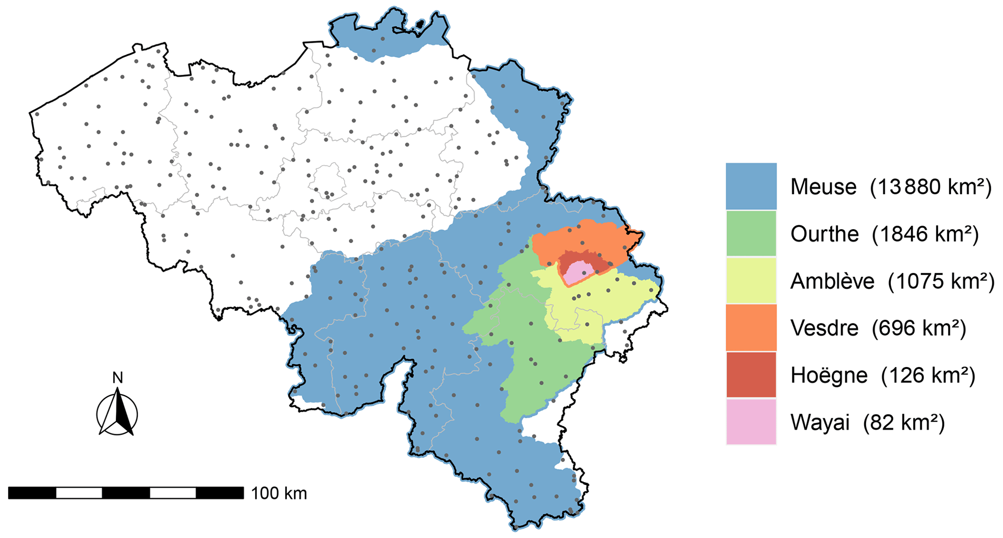
Figure 1Map of Belgium with the definition of the six catchments discussed in this study. Some of these domains are overlapping: the Wayai and Hoëgne catchments are included in the Vesdre catchment; the Vesdre, Ourthe and Amblève catchments are included in the Meuse catchment. The Meuse catchment is limited here to its Belgian part. The dots represent the locations of the rain gauges that provided data during the 2021 mid-July event. The gray lines delimit the Belgian provinces.
After such a disaster, questions arise regarding the role of climate change in the occurrence of this type of event. An attribution study has been rapidly performed (Kreienkamp et al., 2021) and concludes that the likelihood of such an event occurring today at any place over western Europe compared to a 1.2 ∘C cooler climate has increased by a factor of between 1.2 and 9. According to the Clausius–Clapeyron relation, a warmer atmosphere can contain more water vapor, which is expected to increase the intensity and frequency of precipitation events. This type of relationship is, however, difficult to ascertain as the occurrence of such an event is both dynamically and thermodynamically driven (Ludwig et al., 2023; IPCC, 2021; Vergara-Temprado et al., 2021). This makes the attribution of such events to climate change a real challenge, and further analyses are required to address this issue, as in, for instance, Meyer et al. (2022). Such types of analyses strongly rely on the quality of the available observational data.
As described in Mohr et al. (2023), these devastating floods are the result of complex interactions between meteorological, hydrological and hydro-morphological phenomena. An additional aspect that needs to be considered is the presence of dams upstream of some affected valleys in eastern Belgium (Dewals et al., 2021). Multi-disciplinary analyses are required for an in-depth understanding of the course of the events. Investigating the complex dynamics in the affected catchments is necessary to understand the relation between extreme rainfall and the resulting impact. Such analyses require a detailed knowledge of rainfall as the triggering factor of these events. Extremely rare events need to be documented as much as possible, and data must be made available for further studies in hydrology, in urban planning and, more generally, in all multi-disciplinary studies aiming to identify and understand factors leading to such disaster.
Several extreme rainfall and flood events that occurred in the last decades have been documented in the literature. For example, the extraordinary rainfall and flash-flood event which affected the eastern part of the Netherlands in August 2010 is described in Brauer et al. (2011). In Germany, the hydrometeorology of the extreme flood in the Starzel catchment on 2 June 2008 is analyzed in Ruiz-Villanueva et al. (2012). On 8–9 September 2002, a catastrophic flash flood affected the Gard region (France) with maximum 24 h rainfall values of 600–700 mm. This event is extensively documented and analyzed in Delrieu et al. (2005). In Marchi et al. (2010), hydrometeorological data from 25 extreme flash floods across Europe are presented, and a high-resolution dataset of rainfall and discharge observations for 49 events in Europe and the Mediterranean region from 1991 to 2015 is described in Amponsah et al. (2018). All these studies underline the importance of rainfall observations at high spatial and temporal resolutions for the post-analysis of extraordinary flood events.
In the present paper, the observational rainfall data for Belgium that can be used for such analyses are exposed and made available to the scientific community (Journée et al., 2023; Goudenhoofdt et al., 2023). These data are twofold: (1) in situ observations from high-quality rain gauges and (2) rainfall products based on weather radar observations. The radar data are carefully processed and combined with rain gauge measurements to provide a quantitative estimation of precipitation at high spatial (i.e., 1 km) and temporal (i.e., 5 min and hourly) resolutions. Several analyses of these data are performed to describe the spatial and temporal distribution of rainfall during the event and to illustrate its exceptional character.
The paper is organized as follows. In Sect. 2, the rain gauge data and the radar product available for Belgium during the period from 13 to 16 July 2021 are detailed. Section 3 includes several analyses of these data to discuss the event with regard to its spatial and temporal extent together with its exceptional character. Some conclusions are drawn in Sect. 4.
2.1 Rain gauge data
Several rain gauge networks are deployed in Belgium to continuously monitor rainfall at the ground level. These networks are operated by the Royal Meteorological Institute of Belgium (RMI) and by the Belgian regional hydrological services, i.e., Service Public de Wallonie – Mobilité et Infrastructures (https://hydrometrie.wallonie.be, last access: 24 August 2023) and Vlaamse Milieumaatschappij and Hydrologisch Informatiecentrum (https://www.waterinfo.be/, last access: 24 August 2023). In total, 323 rain gauges located at 308 different sites recorded precipitation quantities during the severe rainfall event of mid-July 2021. The spatial distribution of these 308 sites is illustrated in Fig. 1 by the gray dots. On average over Belgium, this represents a density of 10 measurement sites per 1000 km2. This density is somewhat lower for the Meuse Basin (9 per 1000 km2) and slightly larger for the Vesdre Basin (11.5 per 1000 km2). Among the 323 available devices, 168 weighing rain gauges monitored rainfall in real time with a 5 min time resolution, and 155 manual rain gauges recorded daily precipitation amounts. Manual precipitation observations are made each day at 08:00 LT (local time).
All the recorded rain gauge data were checked manually for possible errors and inconsistencies. This data quality control (QC) analysis is made with the help of maps and time series plots that allow us to compare data from neighboring rain gauges. Comparisons are also made with meteorological radar products. This validation process highlighted that two weighing rain gauges provided zero precipitation data continuously over several hours, which was inconsistent with the heavy rainfall observed by neighboring rain gauges and by the radars during that period. In addition, a few gaps of short duration (usually one or two successive timestamps) were reported in the 5 min time series of some other weighing rain gauges. Estimations derived by inverse distance weighted interpolation (IDW) from neighboring weighing rain gauge data have been considered to correct the two periods of erroneous data, as well as to fill the gaps. Regarding the manual rain gauges, some observers measured the daily precipitation amount at times later than 08:00 LT. As a consequence, the total accumulation during the event was correctly recorded but not properly distributed on each day, thus necessitating adjustments of the daily values. This adjustment is based on the sequence of daily totals of neighboring rain gauges. Globally, the QC analysis led to few interventions for all available rain gauge data and none concerning the rain gauges located in the most severely affected area (i.e., Vesdre basin).
Finally, one should note that rain gauge data are subject to various sources of uncertainties. First, the World Meteorological Organization (WMO) recommends that the measurement uncertainty related to the sensor performance under nominal and recommended exposure stays below 5 % (WMO, 2021a). Second, the close environment of the rain gauge might influence the measurements. Following the WMO siting classification (WMO, 2021b), RMI weighing rain gauges are classified either as class 1 (i.e., reference site) or class 2 (i.e., additional estimated uncertainty added by siting up to 5 %) (Gonzalez Sotelino et al., 2016). No classification is currently available for the other rain gauges considered in this analysis.
2.2 Radar-based rainfall product (RADFLOOD21)
The radar product is obtained after careful processing of the weather radar measurements and merging with validated rain gauge measurements. Some of the main challenges of radar-based precipitation estimation are discussed in detail in Goudenhoofdt and Delobbe (2016). The method is under a continuous improvement process based on research and quality control. In particular, the significant underestimation of the operational product during the flood event has led to several improvements. Additionally, some of the parameters have been optimized for this particular case. The processing steps are explained below.
2.2.1 Weather radar measurements
Radars transmit electromagnetic pulses, typically within a beam width of 1∘. Part of the transmitted power is reflected back to the radar by precipitation. Most radars in Europe perform a full volume scan of the atmosphere at different elevation angles (3D) in about 5 min. Estimating rainfall from radar measurements is a challenge because of the many sources of errors and uncertainties (Fig. 2).

Figure 2Phenomena affecting the radar data quality. Courtesy of Markus Peura (Finnish Meteorological Institute).
The product is based on the 3D reflectivity measurements of the following radars:
-
Helchteren, Vlaamse Milieumaatschappij, Belgium (BEHEL);
-
Jabbeke, Royal Meteorological Institute of Belgium, Belgium (BEJAB)
-
Wideumont, Royal Meteorological Institute of Belgium, Belgium (BEWID)
-
Neuheilenbach, Deutscher Wetterdienst, Germany (DENHB)
-
Essen, Deutscher Wetterdienst, Germany (DEESS)
-
Avesnois, Météo-France, France (FRAVE).
The radars are all C-band dual-polarization radars, except for the Wideumont radar, which was still a single-polarization radar in 2021. Their configuration and data processing can differ significantly. This leads to inhomogeneities between the radars that need to be reduced before producing a composite.
A radar has a typical range of 250 km, but the quality of the measurements tends to decrease with distance. As found by Goudenhoofdt and Delobbe (2016), data within a 100 km radius are generally considered to be appropriate for rainfall estimates of good quality (Fig. 3).
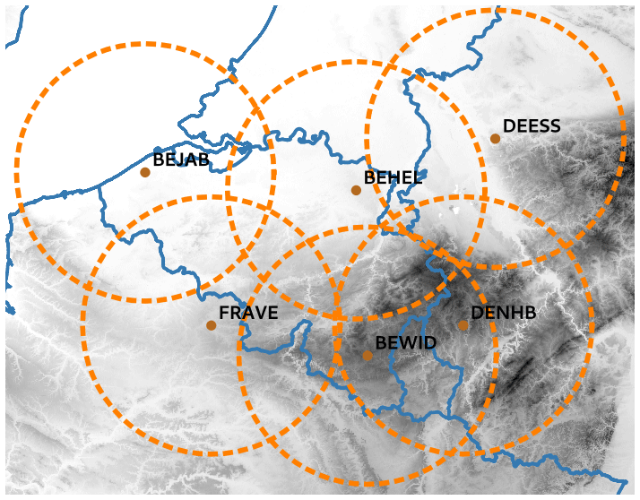
Figure 3Radar coverage with a 100 km radius, country borders and height above sea level (in gray scale from 0 to 1000 m).
2.2.2 Quality control of the radar measurements
The quality control starts by checking the long-term calibration bias of the radar. This uses a basic radar estimation method, with interpolated reflectivity at 800 m above the radar level converted to rain rate using the Marshall–Palmer relationship (Z=200R1.6). An average bias is computed based on comparison with gauge measurements (collocated pixel) over the past 2 months. The method is tuned to ignore all uncertainties and errors not related to calibration errors. The calibration bias is removed before further processing.
Radar measurements over a given area can be permanently or regularly affected by clutter (i.e., non-meteorological echoes) coming from hills or wind farms. This can be solved by removing measurements with an abnormally high frequency of echoes. A new method has been developed to avoid filtering these measurements if their values are significantly larger than the maximum expected clutter level. The goal is to include radar observations as close to the ground as possible without contamination by ground echoes. This is important to mitigate underestimation due to orographic enhancement of precipitation taking place in the lowest layers of the atmosphere. We suspect that this effect was particularly strong during the flood event. The new method is presented in detail in Appendix A.
The radar beam can be partially blocked by elevated areas. The percentage of energy lost is therefore computed. The reflectivity measurements is then corrected accordingly.
The radar measurements can be contaminated by residual non-meteorological echo from planes, wireless devices or the ground in the case of abnormal propagation. Such clutter is identified based on three automatic methods: (1) comparison with the satellite cloudiness product, (2) detection of abnormal changes between measurements at different altitudes (see Appendix B for more details) and (3) detection of unrealistic spatial textures.
2.2.3 Rainfall rate estimation at the ground level
The processing starts with the identification of convective precipitation based on reflectivity gradients. Non-convective precipitation is extrapolated to the ground by using an averaged vertical profile of reflectivity. This allows us, in particular, to mitigate the overestimation caused by melting snow. Missing data after the quality control can be replaced by data from higher radar beams or data in a close neighborhood. The radar reflectivity (Z) is then converted into rain rates (R) taking into account the precipitation type. Only rain has been observed for the current event. The current event was characterized by low to moderately high reflectivity.
The standard Marshall–Palmer (MP) relation is normally applied. Above 40 dBZ, the Deutscher Wetterdienst (DWD) convective relation is used (Z=77R1.9), resulting in lower rain rates with respect to MP. For localized precipitation below 40 dBZ, the US convective relation is used (Z=300R1.4). It also results in lower rain rates compared to MP. A special relation is used for reflectivity below 40 dBZ in areas with orography, where some precipitation enhancement is expected. The NOAA-recommended relation for orography in the western US is used (Z=75R2.0). This results in higher rain rates compared to MP.
2.2.4 Compositing and rainfall accumulation
In order to mitigate the underestimation produced by radar signal attenuation by rainfall along the path, the observations from several radars are combined. Only data from the three closest radars and within a range of 180 km are used here. Data at a very long range with low spatial resolution are not included.
Instantaneous rain rates are obtained every 5 min, corresponding to the full 3D radar scan. The rainfall accumulation over 5 min is obtained by computing the movement of precipitation using optical flow techniques. The combined local–global method is used. Note that the present flood case was not characterized by strong winds. Temporal sampling effects (e.g., jumping cell or ripple effects on the accumulation maps) were therefore very limited. Accumulations over longer durations are obtained by taking the sum of the 5 min accumulations.
2.2.5 Merging with rain gauges
The accumulated rainfall over 1 h is combined with rain gauge measurements from the automatic stations using kriging with external drift (KED) (e.g., Hudson and Wackernagel, 1994). The KED method interpolates the gauge values in a given neighborhood while taking the radar estimation as a linear combination of the expected value of the (Gaussian) process. The method has been tuned for Belgium (see Appendix C). The sliding 1 h spatial correction factor is applied to the 5 min accumulation. This favors the homogeneity of the 5 min products over the consistency with the 1 h products.
3.1 Total rainfall distribution in space
Precipitation accumulations over 3 d, from 13 July, 06:00 UTC, to 16 July, 06:00 UTC, vary largely over Belgium, as illustrated in Fig. 4. While the weather was completely dry during this period in the northwest of Belgium, rainfall accumulations reached almost 300 mm in the eastern part of the country (i.e., the rain gauges recorded up to 291.6 mm). Accumulations over the 3 d period exceeding 200 mm were recorded by four weighing rain gauges (Jalhay, Spa, Mont Rigi and Neu-Hattlich) and by one manual rain gauge (Hockai). These five rain gauges are located in the Province of Liège.
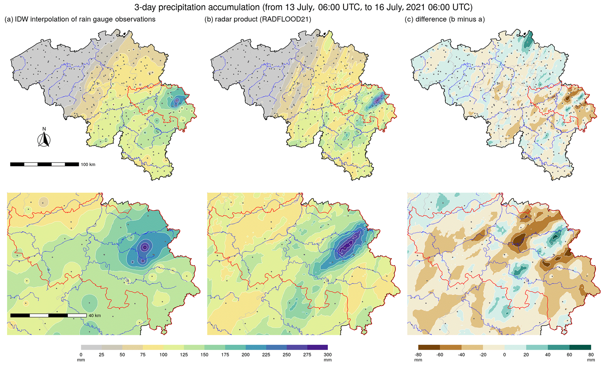
Figure 4Spatial distribution in Belgium (top panels) and in the Province of Liège (bottom panels) of the precipitation accumulation over 3 d (from 13 July, 06:00 UTC, to 16 July, 06:00 UTC). The spatial distribution is derived by inverse distance weighted (IDW) interpolation of all available automatic and manual rain gauge data (a), as well as by the radar product (b). The difference between both estimations is provided in (c). Rain gauge locations are displayed by the gray dots, and the red delimited area corresponds to the Province of Liège.
In Fig. 4, the 3 d precipitation total is mapped over Belgium in two ways. On the one hand, all available 3 d totals recorded by weighing and manual rain gauges are spatially interpolated by an inverse distance weighted (IDW) approach (Fig. 4a). On the other hand, the hourly radar product data are temporally aggregated over the 3 d period (Fig. 4b). Both estimations provide, from a large-scale perspective, comparable rainfall distributions over the country. Differences are, however, noticeable at finer scales. First, the IDW approach tends to give artificial circular patterns around some rain gauges, while radar observations are expected to better capture fine-scale rainfall patterns. Second, the IDW approach is blind in areas with poor density in rain gauges. The difference between both estimations (Fig. 4c) shows that the largest discrepancies are located in an area without any rain gauge in the north of Belgium. Significant differences can also be noted in the eastern part of the Province of Liège, where the precipitation accumulations are the largest and vary strongly over short distances. Such rainfall patterns with large gradients need a very dense network of rain gauges to be accurately captured solely by ground observations. The radar product is thus essential for the spatial analysis of such precipitation events. In particular, the radar product shows that the 3 d precipitation total has exceeded 200 mm for a narrow but elongated area of 265 km2 oriented from southwest to northeast.
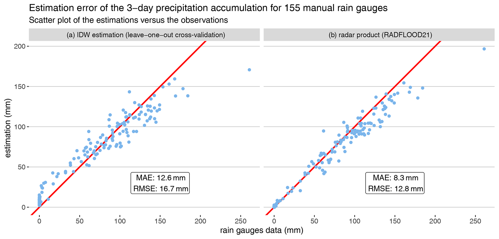
Figure 5Scatter plots of the IDW and radar product estimations versus the observations of the 3 d accumulation for 155 manual rain gauges. The average discrepancies between estimations and observations are summarized by the mean absolute error (MAE) and the root mean square error (RMSE) for both scatter plots.
In order to estimate the uncertainty associated with both spatial distributions of the 3 d precipitation accumulation, a validation analysis is conducted as follows. As the radar product does not integrate observations from manual rain gauges, the 3 d totals from 155 manual rain gauges serve as validation data. For the IDW-derived spatial distribution that relies on both weighing and manual rain gauge data, a leave-one-out cross-validation is applied; i.e., 155 IDW estimations are computed by systematically leaving out one different manual rain gauge item of data, which is used as a reference to evaluate the estimation error. The results are illustrated by scatter plots in Fig. 5. Concerning IDW, these results indicate an overestimation of the smallest values and an underestimation of the largest ones. IDW tends to smooth the spatial distribution of rainfall and attenuates extremes. Regarding the radar product, a rather good match with the manual observations can be noticed for 3 d accumulations till 100 mm. The largest values are, however, generally underestimated. The derived mean absolute error (MAE) and the root mean square error (RMSE) indicate that the radar product nevertheless provides a more accurate spatial distribution of the 3 d accumulation than IDW.
By taking a closer look at the rightmost point of the scatter plots of Fig. 5 (i.e., manual rain gauge with the largest 3 d accumulation), we find an underestimation of almost 25 % by the radar product, while the IDW interpolation of neighboring rain gauges underestimates that specific observation by 35 %. A similar analysis that is focused on daily rainfall totals also highlights that the estimation of the largest values is challenging but better addressed by the radar product. Daily precipitation values above 80 mm, which have been recorded 17 times by manual rain gauges during the 3 d period, are on average underestimated by 16 % by the radar product and by 22 % by the IDW interpolation of neighboring rain gauges.
In order to assess the exceptionality of the precipitation amounts during the event, extreme precipitation statistics derived for Belgium by Van de Vyver (2012, 2013) have been considered. These statistics result from a spatial generalized-extreme-value (GEV) distribution fitted to annual rainfall maxima derived for various accumulation durations and several locations in Belgium from historical precipitation data. Thanks to this spatial approach, extreme precipitation statistics are estimated for any location in Belgium and are currently considered as the reference for, e.g., the design of hydraulic structures. From these statistics, return periods can be associated with the 3 d precipitation accumulations, as illustrated in Fig. 6 for the rainfall distribution estimated by the radar product (i.e., Fig. 4b). Large return periods can be noted for extended areas within Belgium. For instance, the return period estimated for the 3 d total exceeds 50 years for 24.5 % of the Belgian territory (i.e., 7500 km2). The area with a return period estimated to be larger than 100 years covers more than 13 % of the country (i.e., 4000 km2). It should be noted that the extreme-precipitation statistics provided by Van de Vyver (2012, 2013) are here limited to return periods of 200 years as the uncertainty increases considerably when considering return periods significantly larger than the length of the time series. This upper level is exceeded for an area corresponding to 6.5 % of Belgium (i.e., 2000 km2). At some places, the 3 d total considerably exceeds the 200-year return level.

Figure 6Return period estimated for the 3 d precipitation total in Belgium (corresponding to the rainfall distribution estimated by the radar product, i.e., Fig. 4b).
3.2 Rainfall distribution in time
Figure 7 provides a closer look at the rainfall distribution in time for the four weighing rain gauges with a 3 d accumulation over 200 mm. These time series indicate that, for these locations, most of the total rainfall accumulation occurred in a period of approximately 36 h, which is a much shorter period compared to 3 d. It also appears that, within this 36 h period, the hourly precipitation totals were highly variable with several peaks and some hours with almost no precipitation.
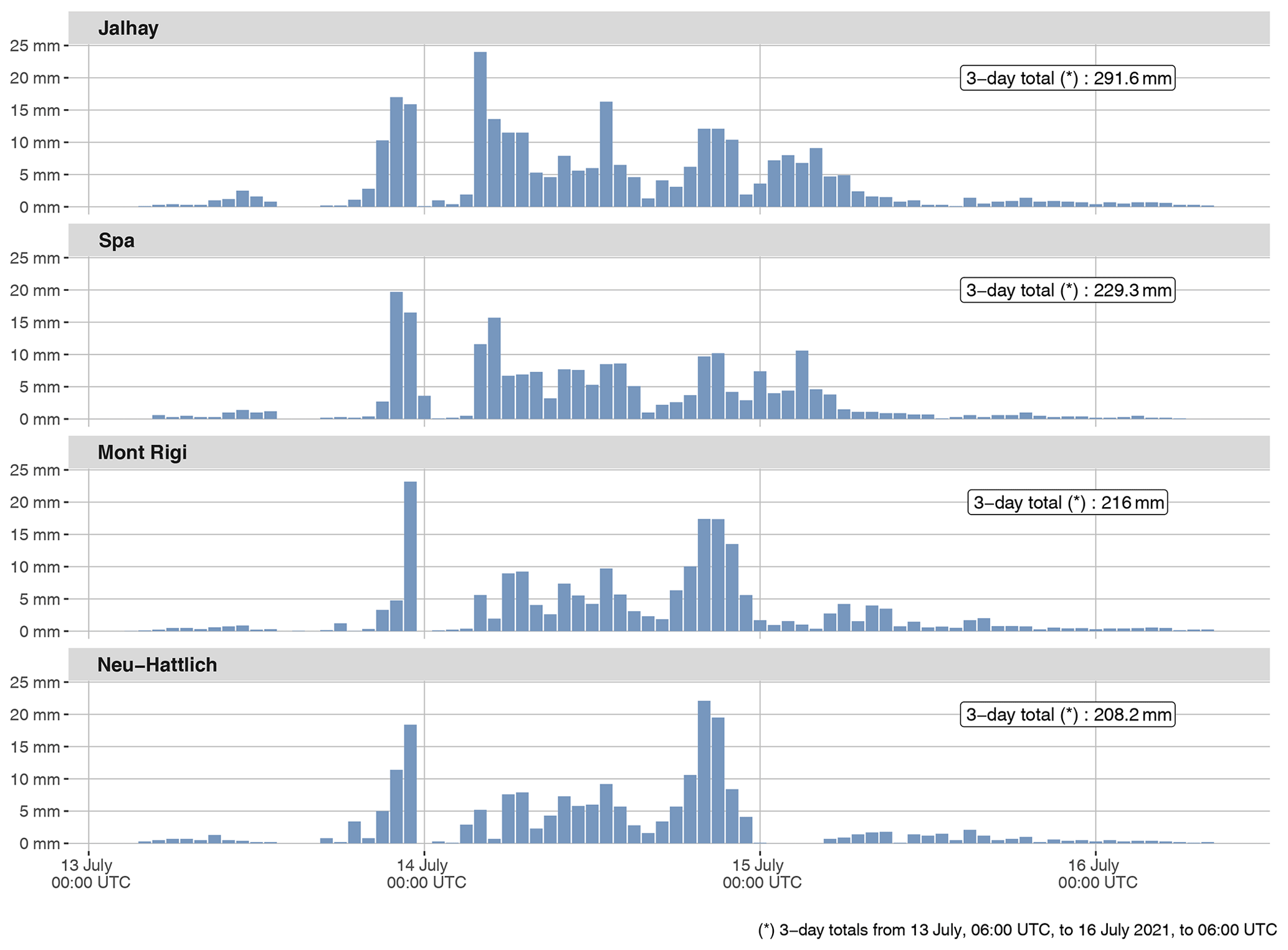
Figure 7Time series of hourly precipitation totals for the four weighing rain gauges with a 3 d accumulation exceeding 200 mm. These four rain gauges are located in the Province of Liège.
For the five manual and weighing rain gauges with the largest 3 d totals (i.e., exceeding 200 mm), the maximum precipitation accumulation for durations from 1 h to 3 d is provided in Fig. 8 and compared against precipitation amounts corresponding to events with return periods from 10 to 200 years, i.e., 10- to 200-year return levels. For these stations, which are all located in the same area of the Province of Liège, precipitation accumulations over short durations till 3 h do not exceed a return period of 30 years. However, the precipitation quantities tend toward extreme levels when increasing the accumulation duration: 6 h accumulations present a return period above 75 years in three places, and 12 h accumulations exceed the 200-year return level at the four weighing rain gauges. For the five considered locations, the exceedance over the 200-year return level is even larger for precipitation accumulations over 1 d and especially over 2 and 3 d: these 2 and 3 d values exceed the 200-year return level by 30 % to 90 % depending on the location. In Jalhay, where the largest 2 and 3 d amounts have been recorded, these 2 and 3 d values correspond to the 200-year return level of rainfall events with a duration of 13 and 15 d, respectively, as can be noted in Dewals et al. (2021).
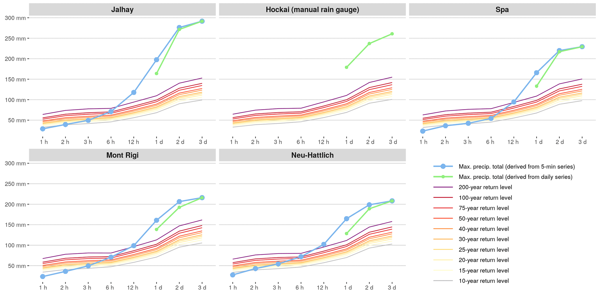
Figure 8Maximum precipitation accumulation between 13 July, 06:00 UTC, to 16 July 2021, 06:00 UTC, for durations from 1 h to 3 d for the five rain gauges with a 3 d accumulation exceeding 200 mm compared against the 10- to 200-year return levels. These maximum values are derived from 5 min time series (weighing rain gauges), as well as from daily time series (weighing and manual rain gauges). These five rain gauges are located in the Province of Liège. The return levels are derived from 10 min historical series for durations up to 12 h and from daily historical series for durations of 1 d or more (Van de Vyver, 2012, 2013).
The analysis of Fig. 8 can be extended to any location in Belgium based on the hourly radar product. For each 1 km pixel of the radar product, the maximum rainfall accumulation is derived for durations from 1 h to 3 d during the period of 13 July, 06:00 UTC, to 16 July, 06:00 UTC. Return periods can then be associated with these precipitation maxima based on the results of Van de Vyver (2012, 2013). Figure 9 summarizes the frequency distribution of these 1 km sampled return periods for the eight considered accumulation durations. The spatial distribution of the estimated return periods for each accumulation duration can be found in Fig. E1. These results indicate that the precipitation accumulations for durations up to 3 h did not reach exceptionally high values anywhere in Belgium (i.e., return period below 30 years). For longer accumulation durations (from 6 h to 3 d), a clear trend towards extreme values can be noticed with, in parallel, an increase in the size of the severely affected areas.
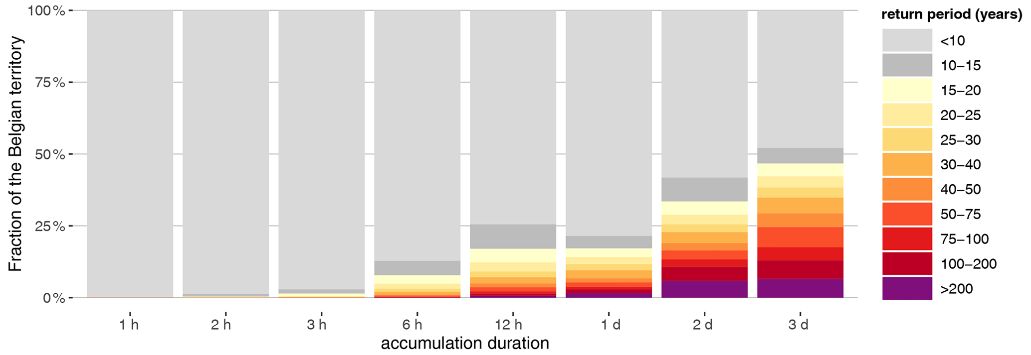
Figure 9Frequency distribution on the Belgian territory of the return period associated with the maximum precipitation accumulation between 13 July, 06:00 UTC, and 16 July 2021, 06:00 UTC, for durations from 1 h to 3 d. The maximum accumulations are derived from hourly (respectively, daily) radar product for durations up to 12 h (respectively, 1, 2 or 3 d). The area of Belgium is 30 688 km2.
Figure 9 illustrates the highly unusual nature of this event. In Belgium, extreme summer rainfall is generally caused by local convective storms, and consequently, extreme return periods are obtained for short durations and concern relatively small areas. In surrounding regions with similar climatic conditions, this type of event is also very rare. A relatively similar event with mixed convective and stratiform rainfall occurred in the Netherlands and the bordering part of Germany in August 2021 (Brauer et al., 2011). Over an area of 740 km2, more than 120 mm of rainfall was recorded in 24 h. Maximum amounts for the whole episode reached 160 mm, which is still lower than the extreme values obtained in the present case.
Long-duration rainfall events, affecting large areas and producing flash floods in several catchments, are relatively common in the Mediterranean and Alpine–Mediterranean regions, as shown in several inventories of European flood events (Gaume et al., 2009; Marchi et al., 2010; Amponsah et al., 2018). However, these events occur mostly in autumn under specific climatic forcing and triggering mechanisms that are not present in our region of interest.
The apparent discontinuity in Fig. 9 from 12 h to 1 d accumulations is related to the temporal granularity of the considered data: maximum accumulations are derived from an hourly radar product for durations up to 12 h and from fixed daily accumulations (from 08:00 to 08:00 LT) for durations of 1, 2 or 3 d in order to be consistent with the extreme-value statistics (Van de Vyver, 2012). The Hershfield factor (van Montfort, 1990) aimed to adjust the impact of the time series granularity when deriving extreme-value statistics is not used to stay as close as possible to the actual statistics.
3.3 Spatio-temporal analysis of the heavy rainfall event
The rainfall distribution in time illustrated in Fig. 7 is limited to the rain gauges with the largest 3 d accumulation, which are all located in the same area (i.e., east of the Province of Liège). Rainfall is, however, differently distributed in time in other areas of Belgium. The sequence of the 5 min radar product (Goudenhoofdt et al., 2023) allows us to grasp the spatiotemporal dynamic of the 3 d event. In complement, maps of 3-hourly precipitation totals derived from the 5 min radar product are provided in Figs. E2 and E3. However, it remains difficult to get an overall insight into the spatial and temporal evolutions of the rainfall patterns during the event from these 5 min or 3-hourly sequences.
Dimensionality reduction methods (Carreira-Perpiñán, 1997; Fodor, 2003; Cunningham, 2008) can be helpful in this context. The goal of dimensionality reduction is to provide a low-dimensional approximation of large data while minimizing the loss of relevant information contained in the data. These approaches thus aim to summarize the essence of the data in a few representative variables. They provide an approximate but easier-to-interpret representation of the data. One of the most popular techniques for dimensionality reduction is principal component analysis (Jolliffe and Cadima, 2016; Wilks, 2011). In this analysis, because of the non-negative character of precipitation data, we will compute a non-negative matrix factorization (NMF) of the 5 min radar product. This NMF analysis will allow us to highlight that rainfall was distributed differently in time over the country. It will provide a synthetic view of the event from which qualitative descriptions can be derived. Background information regarding the NMF method is given in Appendix D.
In order to analyze the 5 min rainfall by NMF, the data first need to be structured in a non-negative m×n matrix V, where each element vij contains the radar value of the pixel i for the timestamp j. This analysis is performed for the 1 km radar pixels located in Belgium (i.e., m=30 669) and the period 13 July, 00:00 UTC, to 16 July, 12:00 UTC (i.e., n=1009). Although NMF approximations of various ranks have been derived, the discussion will be focused on the rank-3 NMF that provides a clear decomposition of the data into three distinct spatiotemporal patterns, as illustrated in Fig. 10. Each component i is composed of a vector wi with values for the m pixels (i.e., spatial pattern of the component i) and a vector hi with values for the n timestamps (i.e., temporal pattern of the component i).
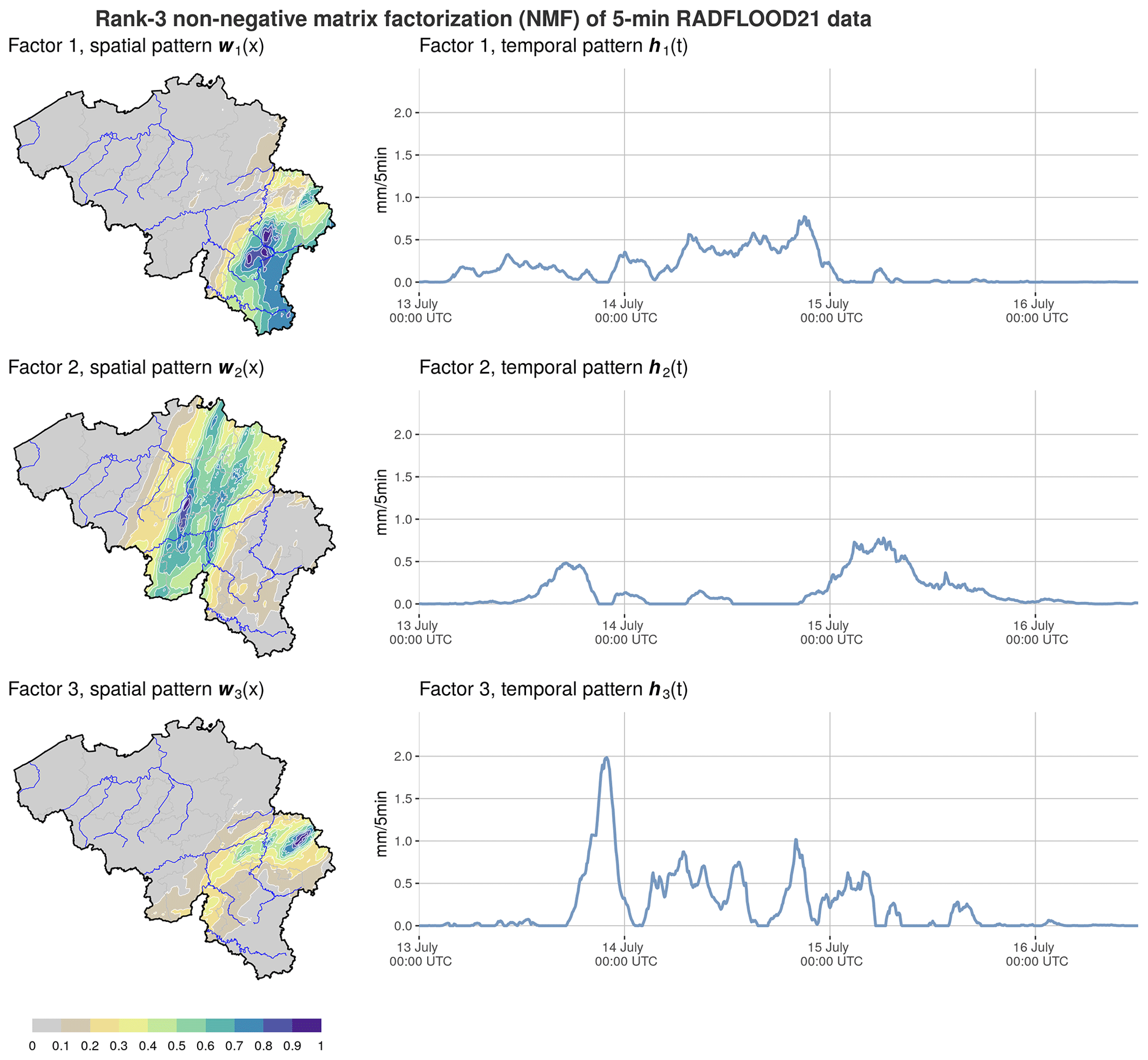
Figure 10Spatial and temporal patterns of the three components resulting from a rank-3 NMF of the 5 min rainfall data.
These results show that NMF provides a decomposition of the rainfall data into three factors with distinct spatiotemporal characteristics. The first factor corresponds to stratiform precipitation in the southeastern part of Belgium that started already in the morning of 13 July and lasted rather continuously till the end of 14 July. The second factor concerns the central part of Belgium with precipitation in the evening of 13 July followed by a rather dry situation on 14 July and more precipitation for the whole of 15 July. Finally, the third factor extracts the heaviest precipitation pattern located in the Province of Liège. This pattern is characterized by successive periods with very intense convective precipitation that started in the evening of 13 July and lasted till the morning of 15 July. The NMF analysis clearly shows that rainfall was distributed differently in time in various areas of the country. In view of the temporal distributions that overlap for the three factors, it is hard to figure out what the dynamical source of these patterns is. This constitutes an interesting future research topic, going beyond the scope of the current data description.
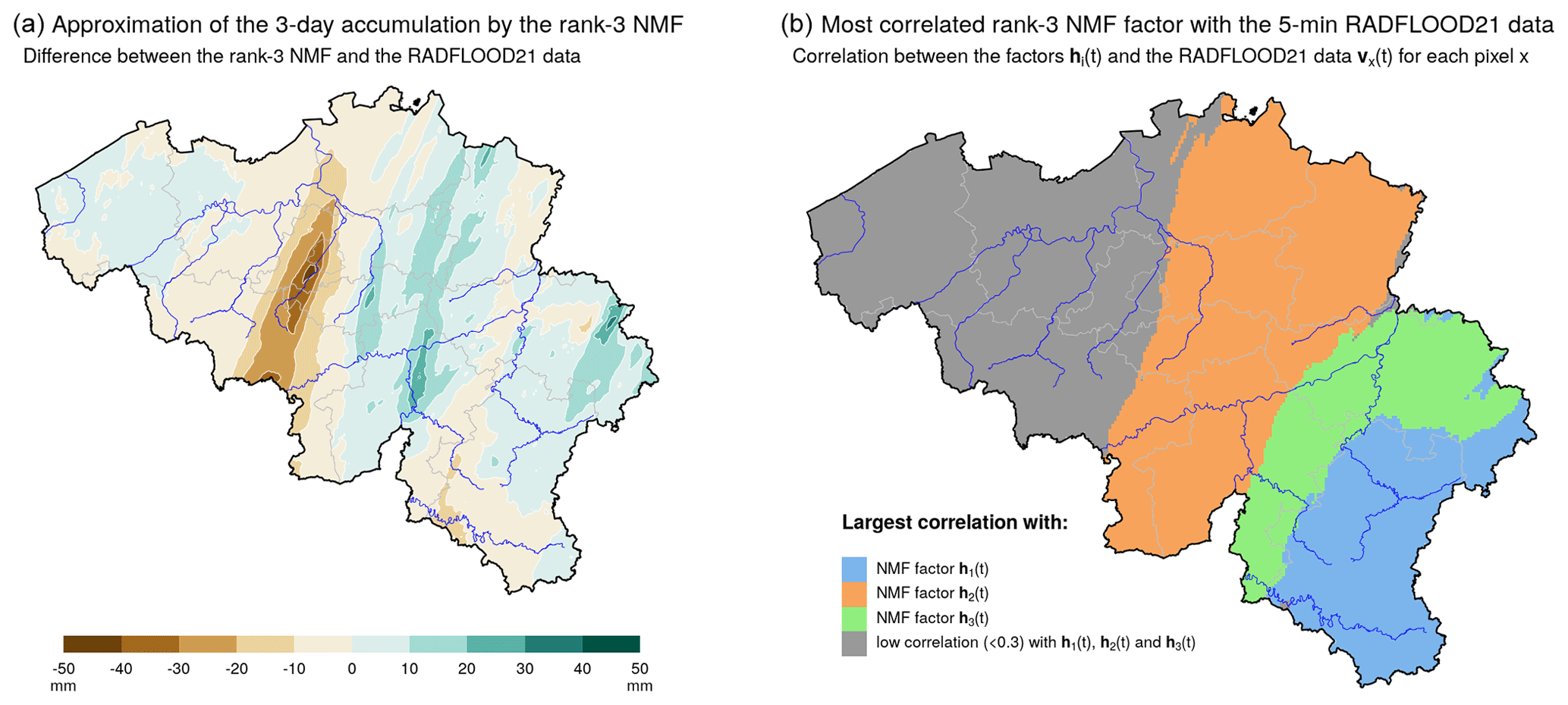
Figure 11(a) Difference in the 3 d accumulation between the rank-3 NMF and the RADFLOOD21 data. (b) Result of the correlation analysis between the rainfall data and the three temporal components hi for each pixel: the map illustrates which component hi is the most correlated with each item of pixel data provided the correlation is larger than 0.3.
The information given in Fig. 11 indicates that the rank-3 NMF approximation provides a meaningful summary of the rainfall data. First, Fig. 11a quantifies how the 3 d accumulation is approximated by the rank-3 NMF. The approximation error is rather low in most places: between −8 % and 16 % where the 3 d accumulation exceeds 100 mm. There is, however, a region in central Belgium with a 3 d accumulation (around 80 mm in the radar product) that is largely underestimated by almost 50 mm in the rank-3 NMF. This is a local pattern that is not captured by the rank-3 NMF but where the 3 d rainfall amounts remain rather moderate. In Fig. 11b, the correlation between the radar product and the three temporal components hi is assessed for each pixel. This analysis confirms that each of these temporal components is mostly correlated with the radar product in distinct geographical areas, which corresponds to the spatial components wi. To conclude, the information provided by the three spatial components wi and the three temporal components hi (i.e., the three maps and three time series of Fig. 10) summarizes well in an easily interpretable way the rainfall data for areas with a 3 d accumulation above 100 mm.
3.4 Analysis of areal averages
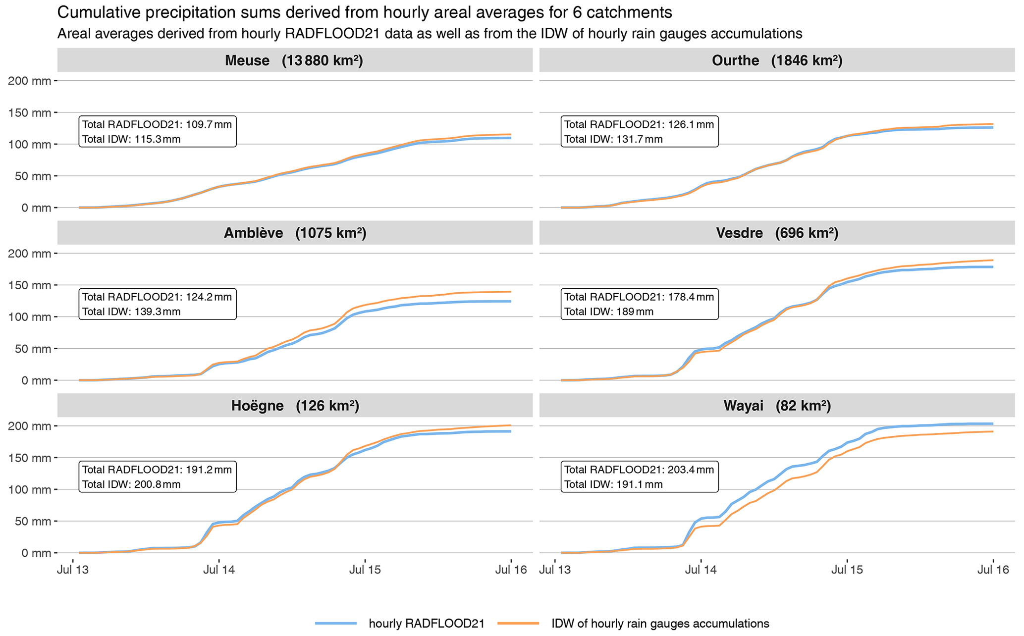
Estimation of areal rainfall averages for catchments may be useful of the hydrological analysis of the event. Such areal averages can easily be derived from the radar product by considering the mean value of all pixels included in the domain of interest. Figure 12 illustrates hourly time series of areal rainfall averages for six catchments of different sizes (defined in Fig. 1). Areal averages derived from the radar product are compared against an alternative estimation solely based on rain gauge data, i.e., an IDW interpolation of hourly rain gauge data at 1 km resolution followed by a spatial aggregation of the interpolation points included in the respective domains. The comparison between both estimations indicates that their difference increases for smaller catchments. Figure 12 also indicates a very large variability in time in terms of hourly rainfall for the Vesdre, Hoëgne and Wayai catchments. This variability in time is significantly smoothed for averages over the large-sized Meuse catchment. By spatially and temporally integrating the radar product, the total precipitation amount that fell over the Belgian part of the Meuse catchment during the 3 d is estimated to be 1.527 km3 (110 mm). Similarly, the total precipitation over the Ourthe and Vesdre catchments is estimated to be 0.240 km3 (130 mm) and 0.125 km3 (180 mm), respectively.
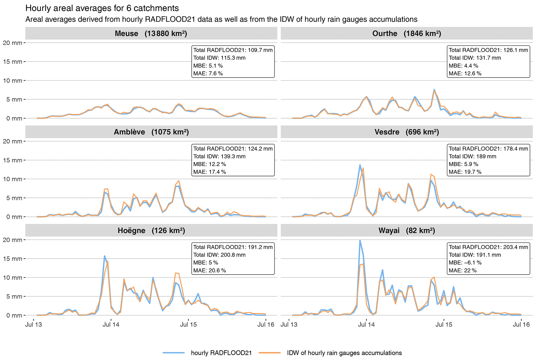
Figure 12Hourly time series of areal rainfall averages for six catchments of different sizes, which are mapped in Fig. 1. The hourly areal averages are derived from the hourly radar product, as well as from hourly rain gauge data (i.e., IDW interpolation of rain gauge data at 1 km resolution followed by a spatial aggregation of the interpolation points included in the respective domains). The difference between both estimations is summarized by the mean bias error (MBE) and the mean absolute error (MAE). The MBE is computed as the average difference between the hourly IDW and RADFLOOD21 estimates (i.e., IDW − RADFLOOD21). Both MBE and MAE are normalized by the average RADFLOOD21 value over the displayed period.
The maximum accumulation for durations from 1 to 72 h derived from these hourly areal time series is provided in Fig. 13 for the six considered catchments. These values increase significantly between 6 and 48 h of accumulation duration. The 48 h totals are estimated to be 100 mm on average over the large-sized catchment of the Meuse and reach almost 200 mm on average for the two smallest catchments of the Hoëgne and Wayai. Cumulative precipitation sums derived from the hourly time series in Fig. 12 are illustrated in Fig. E4 for the interested readers.
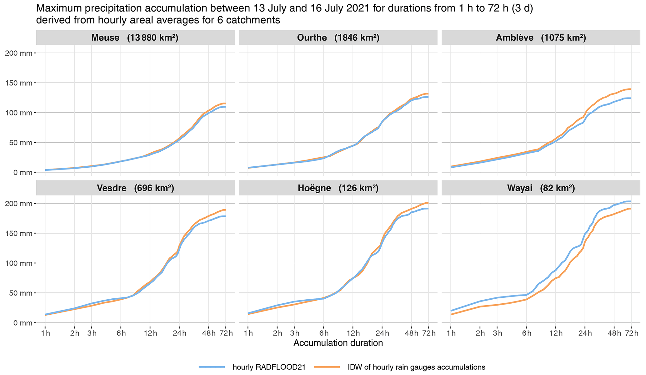
Figure 13Maximum precipitation accumulation for durations from 1 to 72 h by steps of 1 h derived from hourly time series of areal rainfall averages for six catchments of different sizes, which are mapped in Fig. 1. The hourly areal averages are derived from the hourly radar product, as well as from hourly rain gauge data (i.e., IDW interpolation of rain gauge data at 1 km resolution followed by a spatial aggregation of the interpolation points included in the respective domains).
Finally, in order to quantify how the difference between the IDW of rain gauge data and the radar product evolves when they are aggregated in space and time, we considered 67 hydrological catchments in Belgium of various sizes with an average 3 d accumulation exceeding 20 mm. Hourly areal averages were derived for each catchment and then accumulated for various durations till 72 h. For each catchment and accumulation duration, the difference between all pairs of IDW and RADFLOOD21 estimates is characterized by the mean absolute error (MAE) normalized by the mean of the RADFLOOD21 values during the 3 d period. Average MAE values for catchments of similar sizes are finally computed and illustrated in Fig. 14. These results clearly highlight a decrease of the discrepancies between both datasets when the data are aggregated in space over larger domains and accumulated over longer periods.
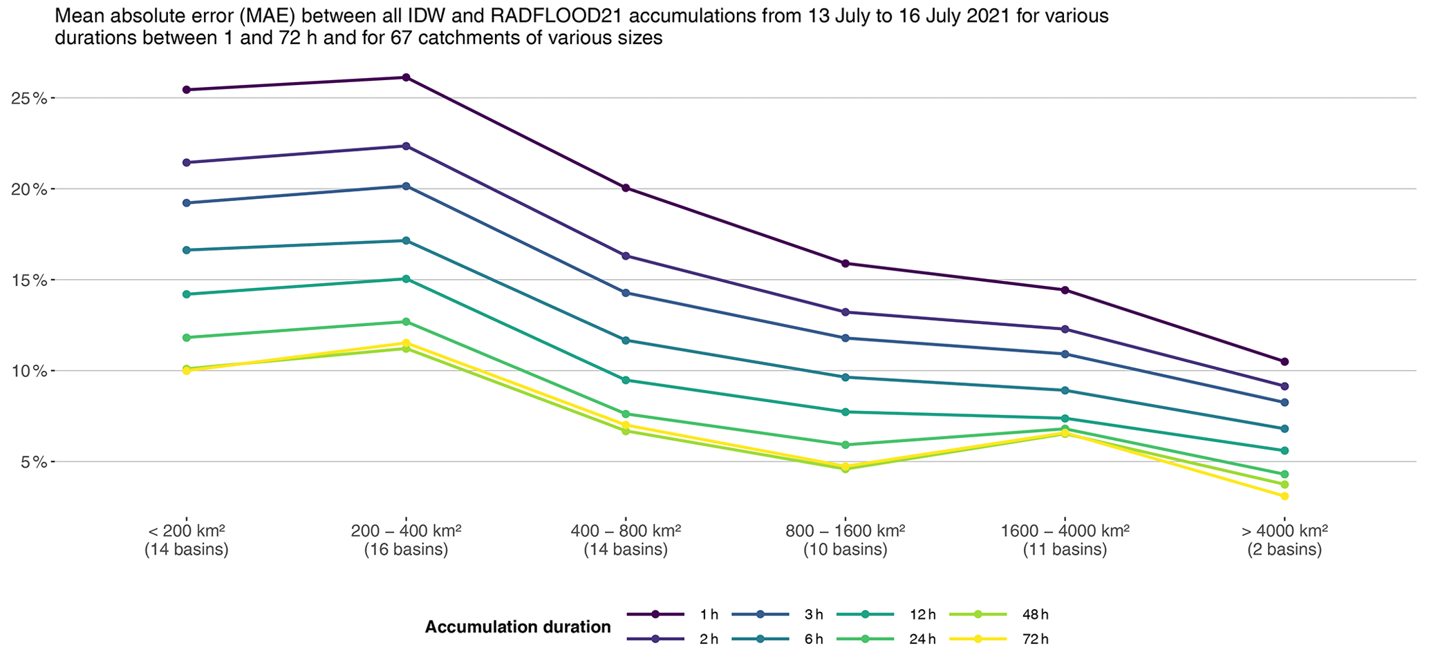
Figure 14Mean absolute error (MAE) between all IDW and RADFLOOD21 accumulations from 13 to 16 July 2021 for various durations between 1 and 72 h and for 67 catchments of various sizes in Belgium (from 61 to 14 800 km2). The 3 d RADFLOOD21 accumulation exceeds 20 mm on areal average for all these catchments. The MAE is normalized per catchment and per accumulation duration by the average RADFLOOD21 value over the 3 d period. Average MAE values for catchments of similar sizes are finally displayed in the figure.
The rainfall event of 13 to 16 July 2021 over central Europe affected considerably the eastern part of Belgium and caused disastrous floods in several river catchments. In order to understand the course of the events and the various factors relating rainfall to flood response, it is essential to obtain the best picture of the spatiotemporal distribution of rainfall. In the present work, we present and analyze quality-controlled rain gauge observations and radar-based rainfall products. The radar products include a merging with automatic gauge measurements. These data are freely available and are provided as a supplement on Zenodo (Journée et al., 2023; Goudenhoofdt et al., 2023).
The most extreme rainfall values were observed in areas with high orography, and estimating rainfall from radar observations is particularly challenging for this event. Radar ground echoes are more frequent and intense in areas with high orography, which affects the quality of the raw radar data. Orographic enhancement is suspected to have played an important role, which makes it important to use radar observations as close to the ground as possible. A proper treatment of ground echoes was therefore essential for this case.
In some areas, fine-scale spatial structures present in the radar-based products differ substantially from those obtained by classical interpolation of rain gauges. Verification shows that errors made by the radar-based product are considerably smaller than those obtained from rain gauge interpolation. For small catchments, incorporating radar observations is required for capturing the temporal evolution of rainfall.
A generic statistical analysis of these data is also provided, allowing for characterization of the return period of such an event and the spatial structure of the precipitation field. This analysis shows that the event of mid-July 2021 is a record-breaking event over most of the eastern part of Belgium, with return periods largely exceeding 50 years. The 200-year return level is exceeded over 2000 km2. The most extreme rainfall over 2 d is almost twice that of the 200-year return level. The analysis of the spatial structure of the rainfall field suggests that there are three dominant spatial structures over Belgium. As these are not well separated in time, additional analyses are needed in order to relate these features to physical processes. Regarding total precipitation amounts integrated over a region during the event, quantities of 0.484 km3 (125 mm) and 1.527 km3 (110 mm) are estimated for the Province of Liẽge and for the Belgian part of the Meuse catchment, respectively.
It is also interesting to note that the return periods are relatively moderate for durations shorter than 6 h. Rainfall temporal evolution cannot be considered to be typical of a flash-flood event. In contrast, according to several testimonies, the response of the system appears to be very close to character of a flash flood, with surprise effects at various levels (Van Camp et al., 2022; Dewals et al., 2021). This points out the high nonlinearity of the system and the fact that various other catchment-specific parameters like topography, land use or soil properties played an important role. Additional processes like the transport of debris by fast-flowing water need to be considered to understand the relation between precipitation and flood response. The presence of dams in some valleys affected by floods should also be taken into account.
The data sets presented here have been produced and quality-controlled with the utmost care. Nevertheless, some additional work can be performed to further refine rainfall estimates. The radar-based rainfall product used in the present study is based on single-polarization radar information only. The exploitation of polarimetric information available from the dual-polarization radars covering the area of interest could bring some additional benefits. Extending the area of interest and incorporating additional information from radars and rain gauge networks available in neighboring countries could be realized in an international effort to produce the best picture of this event over the full area affected by floods.
The usage of high-quality rainfall data of extreme events is of great interest in many fields. Besides the question of the impact of climate change on the occurrence of such events, many questions arise related to water resource and flood risk management or land use planning. Understanding the full causality chain from rainfall to floods and further to the resulting impact in terms of casualties and economic losses is a challenging multidisciplinary enterprise. The present work is a contribution to this global effort.
A1 Doppler filtering
The radar signal processor includes a Doppler filter for removing clutter. The Wideumont radar filter is a time domain infinite impulse response filter. The more recent Jabbeke and Helchteren radars include a frequency domain filtering which computes the power spectrum using a discrete Fourier transform (DFT). The time domain filter only suppresses the signal in the filtered region, while the DFT filter is also designed to restore the weather signal in the filtered region. In addition, the processing chain includes threshold checks to remove data of low quality. The clutter correction ratio (CCOR) is defined as the logarithmic ratio between the unfiltered signal power and the clutter-filtered signal power. The CCOR for each range gate is compared with a user-set threshold, and data with CCORs above this threshold are set as invalid.
A2 Computation of the static-clutter map
A measurement location is considered to be systematically contaminated by non-meteorological echoes (clutter) if
-
its height is below 1200 m above the radar level,
-
its distance from the radar is below 100 km, and
-
its frequency of exceeding 7 dBZ is above 20 % for a given period.
For the sake of consistency, the static-clutter map is smoothed to remove small holes with valid data.
A3 Computation of static-clutter-level statistics
The frequency distribution of the reflectivity is computed by bins of 5 dB.
In most cases, the fixed target causes a signal with a relatively constant reflectivity. This corresponds to the bin with the highest frequency. It is considered to be the mean clutter level.
Some targets, like wind farms, can cause a fluctuating signal, and the mean statistics are useless. For a given reflectivity bin, one can determine if its frequency is unrealistic in the current Belgian climatic conditions. By taking the upper bound of the highest unrealistic bin, one obtains the maximum detectable clutter level.
The unrealistic frequencies have been optimized by trial and error using several years of data. The results can be found in Table A1.
A4 Identification of static clutter
A reflectivity measurement is considered to be static clutter if
-
it belongs to the static-clutter map computed in the last 2 months, and
-
its value is not 5 dB above the maximum clutter level computed in the last 2 months.
Therefore, an actual rainfall value is kept if it is sufficiently large.
A5 Handling of false zeros
The CCOR threshold is set to 30 dB for the Jabbeke and Helchteren radars and 15 dB for the Wideumont radar. When the Doppler filter removes more than this threshold, the reflectivity is improperly set to undetected by the radar processing (which means zero precipitation). Other kinds of processing from all radars also introduce false zeros. This is problematic since the static-clutter statistics cannot be computed reliably anymore. The only guaranteed solution is to use a static-clutter map and maximum clutter level based on unfiltered reflectivity.
Using the unfiltered statistics results in a significant reduction of the filter performance. To keep some efficiency, a value which is valid for the filtered statistics and which exceeds the unfiltered mean clutter level minus the CCOR threshold is not rejected.
Some residual clutter might remain at this stage, but the clutter processing further includes dynamical filters based on satellite cloudiness, vertical profiles of reflectivity and spatial texture (see Sect. 2.2.2).
A6 Results
Figures A1 and A2 show an example of the static-clutter map and statistics for the radar of Helchteren, valid during the flood event, in the Vesdre catchment. It can be seen that a significant part of the area is affected by strong clutter. The Doppler filtering is very efficient, and some high precipitation values can be retrieved.
Table A1Shown here is, for a given reflectivity level, the minimum frequency which will never be reached by precipitation only under the current Belgian climatic conditions.

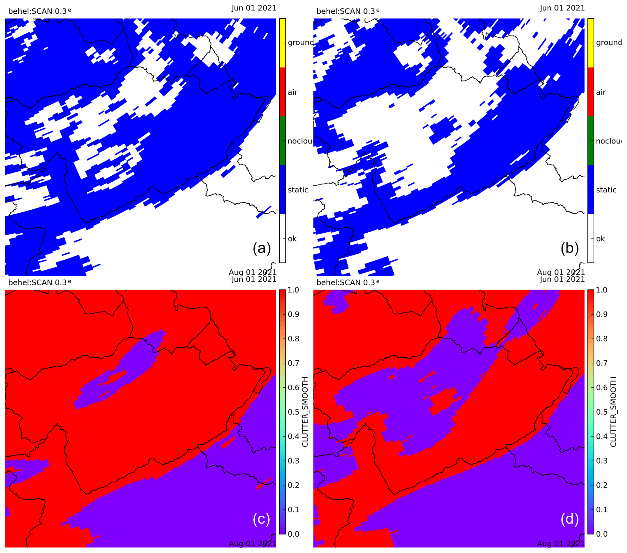
Figure A1Static-clutter map for the unfiltered (a, c) and filtered (b, d) reflectivity before (a, b) and after (c, d) smoothing. The map is centered on the Vesdre catchment.
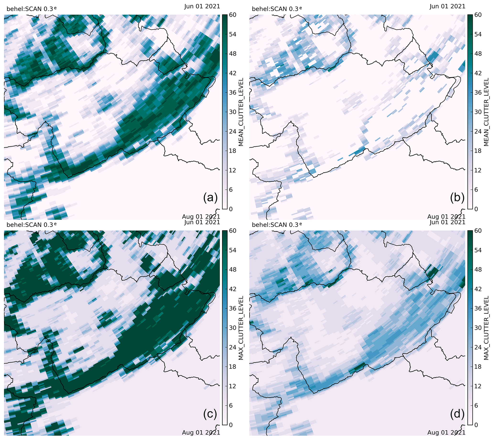
Figure A2Mean (a, b) and maximum (c, d) clutter level for the unfiltered (a, c) and filtered (b, d) reflectivity. The map is centered on the Vesdre catchment.
A measurement at a given elevation is considered to be clutter (non-meteorological) if the gradient between its value and the corresponding (horizontally) interpolated value on a higher (lower) elevation exceeds −20 dBZ km−1 (+10 dBZ km−1) in magnitude. Because of variations from signal fluctuations, a minimum absolute difference of 5 dBZ between two corresponding values at different elevations is required for clutter identification.
The KED method has been tuned on Belgian rainfall. Here are the main parameters.
-
interpolation of the four closest radar values at the gauge location
-
spherical covariance model for the residual error with a range of 20 km
-
correlation limited to 70 % in a 1 km neighborhood due to sampling and measurement errors
-
square root transformation to ensure Gaussianity
-
use of the 21 nearest gauges for a given location
-
not valid locally if there are fewer than four gauge values above 0.1 mm
-
not valid locally if the correlation (R2) between the radar and gauge is below 0.5
-
invalid data replaced by a single-gauge bias correction
-
smooth transition to a single-gauge bias correction outside the convex hull
Given a data matrix V with m rows and n columns (i.e., a matrix of dimension m×n) and with non-negative elements vij≥0 (i.e., V is a non-negative matrix), the non-negative matrix factorization (NMF) approximates V as the product of two non-negative matrices W and H of dimensions m×k and k×n, respectively:
The approximation (Eq. D1) of V can equivalently be written with vectors instead of matrices by
where wi (respectively, hi) of dimension m×1 (respectively, 1×n) denotes the ith column of W (respectively, the ith row of H). Equation (D2) formulates the approximation of V as the sum of k matrices of rank 1 (i.e., the matrix product of two vectors), which are called components or features. In practice, k is set to be much smaller than the dimensions m and n in order to decompose V into a limited number of components that are expected to represent meaningful characteristics of the original data. NMF is generally solved as an optimization problem, where an objective function characterizing the difference between V and matrix product WH has to be minimized. Various algorithms for NMF have been proposed in the literature. In this analysis, we used the algorithm rNMF (Sun et al., 2013), which is available as an R package. We refer to Gillis (2020) for more detailed information about NMF.
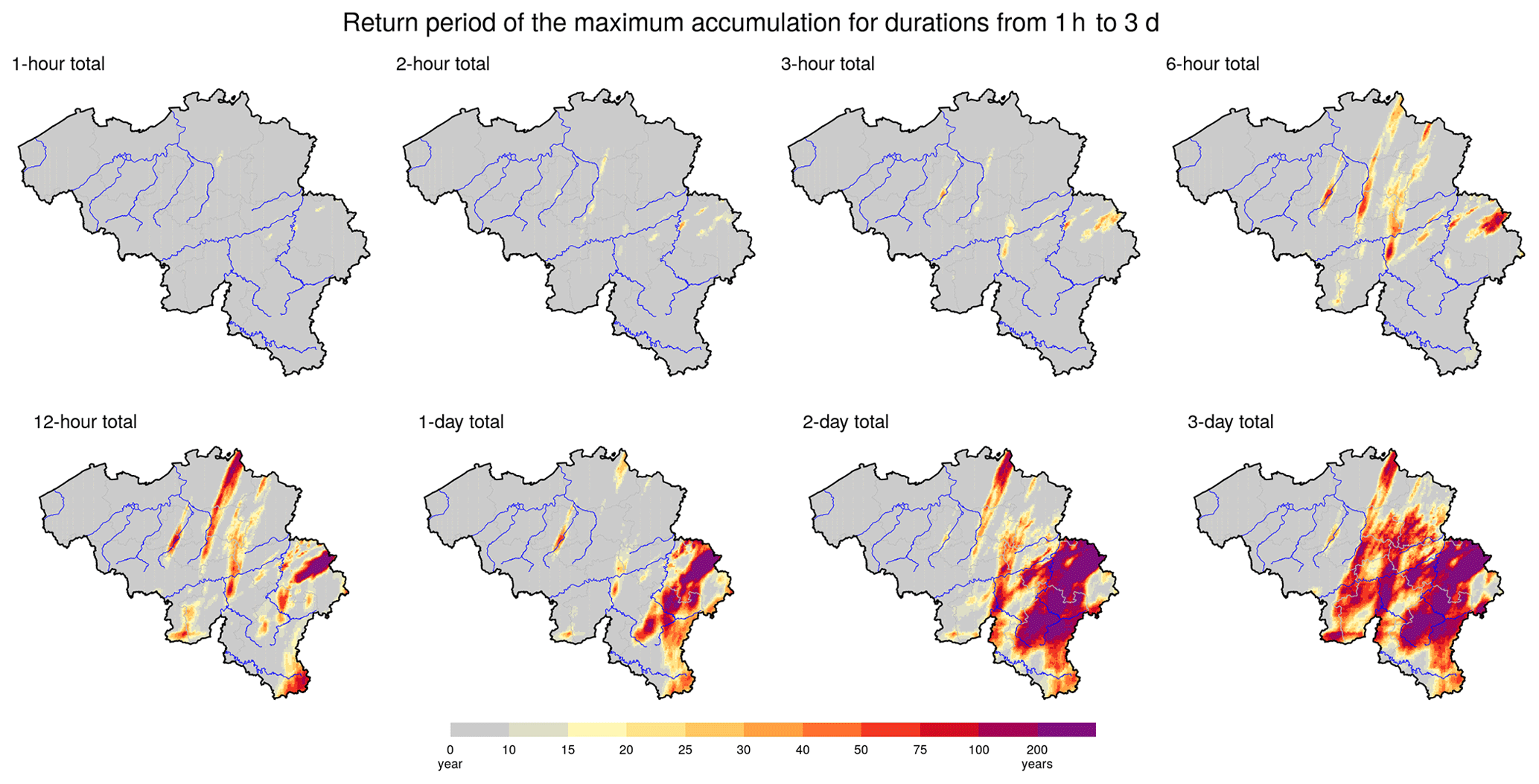
Figure E1Return period estimated for the maximum precipitation accumulation between 13 July, 06:00 UTC, to 16 July 2021, 06:00 UTC, for durations from 1 h to 3 d. The maximum accumulations are derived from hourly (respectively, daily) radar product data for durations up to 12 h (respectively, durations of 1, 2 or 3 d).
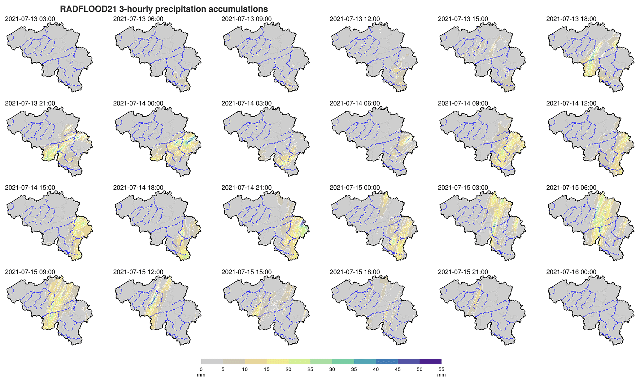
Figure E2The 3-hourly precipitation accumulations in Belgium derived from the 5 min radar product data. The timestamp on top of each map indicates the end of the 3 h period in UTC.
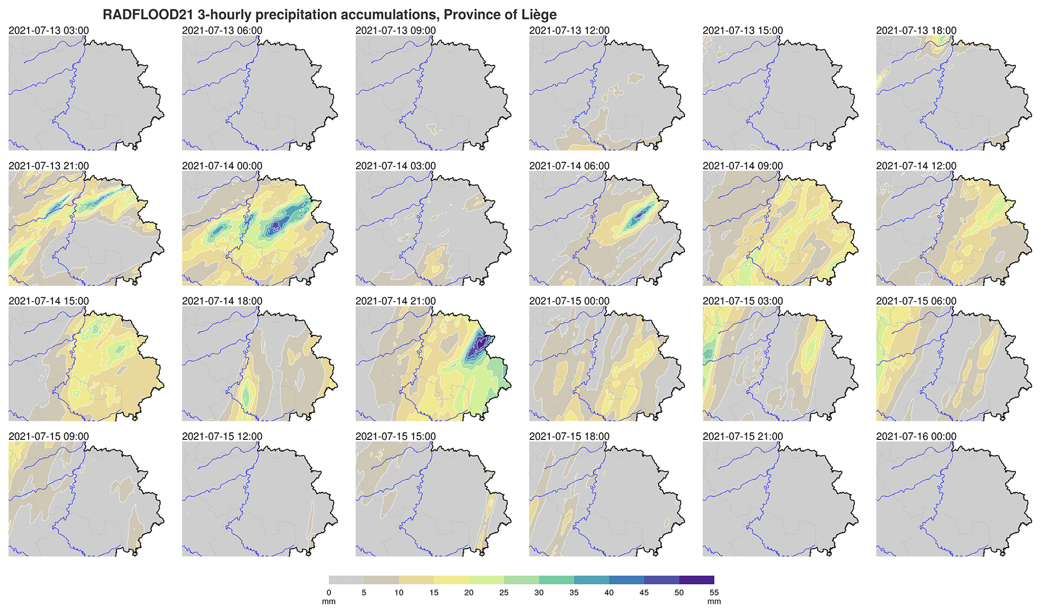
Figure E3The 3-hourly precipitation accumulations in the Province of Liège derived from the 5 min radar product data. The timestamp on top of each map indicates the end of the 3 h period in UTC.
The discussed rain gauge data and radar product RADFLOOD21 can be accessed on Zenodo (https://doi.org/10.5281/zenodo.7739983, Journée et al., 2023; https://doi.org/10.5281/zenodo.7740059, Goudenhoofdt et al., 2023.
MJ extracted and verified the rain gauge data; EG developed the radar product RADFLOOD21; MJ analyzed the data; MJ, EG, SV and LD wrote the paper.
The contact author has declared that none of the authors has any competing interests.
Publisher's note: Copernicus Publications remains neutral with regard to jurisdictional claims in published maps and institutional affiliations.
The authors thank Ruben Imhoff and Wolfgang Wagner for their careful review of the paper. Their constructive comments and suggestions were greatly appreciated. This study makes use of recordings from rain gauges operated by the following Belgian regional hydrological services: Service Public de Wallonie – Mobilité et Infrastructures (https://hydrometrie.wallonie.be, last access: 24 August 2023), Vlaamse Milieumaatschappij (https://www.waterinfo.be/, last access: 24 August 2023) and Hydrologisch Informatiecentrum (https://www.waterinfo.be/, last access: 24 August 2023). Radar observations from Vlaamse Milieumaatschappij, the German Weather Service and Météo-France were used as well. All teams responsible for the maintenance and operation of rain gauge and radar networks in Belgium and the neighboring countries are warmly thanked.
This paper was edited by Adriaan J. (Ryan) Teuling and reviewed by Ruben Imhoff and Wolfgang Wagner.
Amponsah, W., Ayral, P.-A., Boudevillain, B., Bouvier, C., Braud, I., Brunet, P., Delrieu, G., Didon-Lescot, J.-F., Gaume, E., Lebouc, L., Marchi, L., Marra, F., Morin, E., Nord, G., Payrastre, O., Zoccatelli, D., and Borga, M.: Integrated high-resolution dataset of high-intensity European and Mediterranean flash floods, Earth Syst. Sci. Data, 10, 1783–1794, https://doi.org/10.5194/essd-10-1783-2018, 2018. a, b
Assuralia: Actualisation relative aux inondations de juillet 2021, https://press.assuralia.be/actualisation-relative-aux-inondations-de-juillet-2021 (last access: 3 February 2023), 2022. a
Brauer, C. C., Teuling, A. J., Overeem, A., van der Velde, Y., Hazenberg, P., Warmerdam, P. M. M., and Uijlenhoet, R.: Anatomy of extraordinary rainfall and flash flood in a Dutch lowland catchment, Hydrol. Earth Syst. Sci., 15, 1991–2005, https://doi.org/10.5194/hess-15-1991-2011, 2011. a, b
Carreira-Perpiñán, M.: A Review of Dimension Reduction Techniques, Technical Report CS-96-09, Department of Computer Science, University of Sheffield, Sheffield, UK, https://www.cse-lab.ethz.ch/wp-content/uploads/2018/03/DimensionReductionBrifReview.pdf, (last access: 24 August 2023), 1997. a
Cunningham, P.: Dimension Reduction, Springer, 91–112, https://doi.org/10.1007/978-3-540-75171-7_4, 2008. a
Delrieu, G., Nicol, J., Yates, E., Kirstetter, P.-E., Creutin, J.-D., Anquetin, S., Obled, C., Saulnier, G.-M., Ducrocq, V., Gaume, E., Payrastre, O., Andrieu, H., Ayral, P.-A., Bouvier, C., Neppel, L., Livet, M., Lang, M., du Châtelet, J. P., Walpersdorf, A., and Wobrock, W.: The Catastrophic Flash-Flood Event of 8–9 September 2002 in the Gard Region, France: A First Case Study for the Cévennes–Vivarais Mediterranean Hydrometeorological Observatory, J. Hydrometeorol., 6, 34–52, https://doi.org/10.1175/JHM-400.1, 2005. a
Dewals, B., Erpicum, S., Pirotton, M., and Archambeau, P.: The July 2021 extreme floods in the Belgian part of the Meuse, Hydrolink Magazine, https://hdl.handle.net/20.500.11970/109527 (last access: 24 August 2023), 2021. a, b, c, d
Fodor, I.: A survey of dimension reduction techniques, Tech. Rep. UCRL-ID-148494, US Department of Energy Office of Scientific and Technical Information, https://doi.org/10.2172/15002155, 2003. a
Gaume, E., Bain, V., Bernardara, P., Newinger, O., Barbuc, M., Bateman, A., Blaškovičová, L., Blöschl, G., Borga, M., Dumitrescu, A., Daliakopoulos, I., Garcia, J., Irimescu, A., Kohnova, S., Koutroulis, A., Marchi, L., Matreata, S., Medina, V., Preciso, E., Sempere-Torres, D., Stancalie, G., Szolgay, J., Tsanis, I., Velasco, D., and Viglione, A.: A compilation of data on European flash floods, J. Hydrol., 367, 70–78, https://doi.org/10.1016/j.jhydrol.2008.12.028, 2009. a
Gillis, N.: Nonnegative Matrix Factorization, Society for Industrial and Applied Mathematics, Philadelphia, PA, https://doi.org/10.1137/1.9781611976410, 2020. a
Gonzalez Sotelino, L., De Coster, N., Beirinckx, P., and Peeters, P.: Environmental Classification of RMI Automatic Weather Station Network, in: WMO TECO 2016 Conference, WMO TECO Conference, Madrid, Spain, 27–30 September 2006, https://www.wmocimo.net/eventpapers/session1/posters1/P1(14)_sotelino.pdf (last access: 24 August 2023), 2016. a
Goudenhoofdt, E. and Delobbe, L.: Generation and Verification of Rainfall Estimates from 10-Yr Volumetric Weather Radar Measurements, J. Hydrometeorol., 17, 1223–1242, https://doi.org/10.1175/jhm-d-15-0166.1, 2016. a, b
Goudenhoofdt, E., Journée, M., and Delobbe, L.: Observational rainfall data of the 2021 mid-July flood event in Belgium – Part 2. Radar product RADFLOOD21, Zenodo [data set], https://doi.org/10.5281/zenodo.7740059, 2023. a, b, c, d, e
Gouvernement Wallon: Inondations de juillet 2021: bilan et perspectives, https://www.wallonie.be/fr/actualites/inondations-de-juillet-2021-bilan-et-perspectives (last access: 1 February 2023), 2022. a
Hudson, G. and Wackernagel, H.: Mapping temperature using kriging with external drift: Theory and an example from scotland, Int. J. Climatol., 14, 77–91, https://doi.org/10.1002/joc.3370140107, 1994. a
IPCC: Climate Change 2021: The Physical Science Basis, in: Contribution of Working Group I to the Sixth Assessment Report of the Intergovernmental Panel on Climate Change, Cambridge: Cambridge University Press, https://doi.org/10.1017/9781009157896, 2023. a
Jolliffe, I. and Cadima, J.: Principal component analysis: A review and recent developments, Philos. T. Roy. Soc. A, 374, 20150202, https://doi.org/10.1098/rsta.2015.0202, 2016. a
Journée, M., Goudenhoofdt, E., and Delobbe, L.: Observational rainfall data of the 2021 mid-July flood event in Belgium – Part 1. Rain gauges observations, Zenodo [data set], https://doi.org/10.5281/zenodo.7739983, 2023. a, b, c, d
Kreienkamp, F., Philip, S. Y., Tradowsky, J. S., Kew, S. F., Lorenz, P., Arrighi, J., Belleflamme, A., Bettmann, T., Caluwaerts, S., Chan, S. C., Ciavarella, A., De Cruz, L., de Vries, H., Demuth, N., Ferrone, A., Fischer, R. M., Fowler, H. J., Goergen, K., Heinrich, D., Henrichs, Y., Lenderink, G., Kaspar, F., Nilson, E., Otto, F. E. L., Ragone, F., Seneviratne, S. I., Singh, R. K., Skålevåg, A., Termonia, P., Thalheimer, L., van Aalst, M., Van den Bergh, J., Van de Vyver, H., Vannitsem, S., van Oldenborgh, G. J., Van Schaeybroeck, B., Vautard, R., Vonk, D., and Wanders, N.: Rapid attribution of heavy rainfall events leading to the severe flooding in Western Europe during July 2021, https://www.worldweatherattribution.org/wp-content/uploads/Scientific-report-Western-Europe-floods-2021-attribution.pdf (last access: 24 August 2023), 2021. a, b
Ludwig, P., Ehmele, F., Franca, M. J., Mohr, S., Caldas-Alvarez, A., Daniell, J. E., Ehret, U., Feldmann, H., Hundhausen, M., Knippertz, P., Küpfer, K., Kunz, M., Mühr, B., Pinto, J. G., Quinting, J., Schäfer, A. M., Seidel, F., and Wisotzky, C.: A multi-disciplinary analysis of the exceptional flood event of July 2021 in central Europe – Part 2: Historical context and relation to climate change, Nat. Hazards Earth Syst. Sci., 23, 1287–1311, https://doi.org/10.5194/nhess-23-1287-2023, 2023. a
Marchi, L., Borga, M., Preciso, E., and Gaume, E.: Characterisation of Selected Extreme Flash Floods in Europe and Implications for Flood Risk Management, J. Hydrol., 394, 118–133, https://doi.org/10.1016/j.jhydrol.2010.07.017, 2010. a, b
Meyer, J., Neuper, M., Mathias, L., Zehe, E., and Pfister, L.: Atmospheric conditions favouring extreme precipitation and flash floods in temperate regions of Europe, Hydrol. Earth Syst. Sci., 26, 6163–6183, https://doi.org/10.5194/hess-26-6163-2022, 2022. a
Mohr, S., Ehret, U., Kunz, M., Ludwig, P., Caldas-Alvarez, A., Daniell, J. E., Ehmele, F., Feldmann, H., Franca, M. J., Gattke, C., Hundhausen, M., Knippertz, P., Küpfer, K., Mühr, B., Pinto, J. G., Quinting, J., Schäfer, A. M., Scheibel, M., Seidel, F., and Wisotzky, C.: A multi-disciplinary analysis of the exceptional flood event of July 2021 in central Europe – Part 1: Event description and analysis, Nat. Hazards Earth Syst. Sci., 23, 525–551, https://doi.org/10.5194/nhess-23-525-2023, 2023. a, b, c
MunichRe: Hurricanes, cold waves, tornadoes: Weather disasters in USA dominate natural disaster losses in 2021, Europe: Extreme flash floods with record losses, https://www.munichre.com/en/company/media-relations/media-information-and-corporate-news/media-information/2022/natural-disaster-losses-2021.html (last access: 20 December 2022), 2022. a
Ruiz-Villanueva, V., Borga, M., Zoccatelli, D., Marchi, L., Gaume, E., and Ehret, U.: Extreme flood response to short-duration convective rainfall in South-West Germany, Hydrol. Earth Syst. Sci., 16, 1543–1559, https://doi.org/10.5194/hess-16-1543-2012, 2012. a
Sun, J., Xu, Y., Lopiano, K., and Young, S.: Robust Non-Negative Matrix Factorization Procedures for Analyzing Tumor and Face Image Data, in: Proceedings of the Joint Statistical Meetings, Joint Statistical Meetings, Boston, Massachusetts, 2–7 August 2014, https://www.researchgate.net/publication/263039018_Robust_Non-Negative_Matrix_Factorization_Procedures_for_Analyzing_Tumor_and_Face_Image_Data (last access: 24 August 2023), 2013. a
Van Camp, M., de Viron, O., Dassargues, A., Delobbe, L., Chanard, K., and Gobron, K.: Extreme Hydrometeorological Events, a Challenge for Gravimetric and Seismology Networks, Earth's Future, 10, e2022EF002737, https://doi.org/10.1029/2022EF002737, 2022. a, b
Van de Vyver, H.: Spatial regression models for extreme precipitation in Belgium, Water Resour. Res., 48, W09549, https://doi.org/10.1029/2011wr011707, 2012. a, b, c, d, e
Van de Vyver, H.: Practical return level mapping for extreme precipitation in Belgium, RMI scientific and technical publication, 30 pp., 2013. a, b, c, d
van Montfort, M.: Sliding maxima, J. Hydrol., 118, 77–85, https://doi.org/10.1016/0022-1694(90)90251-r, 1990. a
Vergara-Temprado, J., Ban, N., Ban, N., and Schär, C.: Extreme Sub‐Hourly Precipitation Intensities Scale Close to the Clausius‐Clapeyron Rate Over Europe, Geophys. Res. Lett., 48, e2020GL08950, https://doi.org/10.1029/2020gl089506, 2021. a
Wilks, D. S.: Statistical Methods in the Atmospheric Sciences, in: vol. 100, Elsevier Academic Press, Amsterdam, Boston, ISBN 9780123850225, 2011. a
WMO: Operational Measurement Uncertainty Requirements and Instrument Performance Requirements, Annex 1.A. of the guide to meteorological instruments and methods of observation (CIMO guide), WMO No. 8, Vol. 1, Secretariat of the World Meteorological Organization, Geneva, Switzerland, https://library.wmo.int/index.php?id=12407&lvl=notice_display (last accessed: 24 August 2023), 2021a. a
WMO: Siting Classifications for Surface Observing Stations on Land, Annex 1.D. of the guide to meteorological instruments and methods of observation (CIMO guide), WMO No. 8, Vol. 1, Secretariat of the World Meteorological Organization, Geneva, Switzerland, https://library.wmo.int/index.php?id=12407&lvl=notice_display (last access: 24 August 2023), 2021b. a
- Abstract
- Introduction
- Precipitation data
- Quantitative rainfall analysis
- Conclusions
- Appendix A: Filtering of static non-meteorological radar echoes
- Appendix B: Filtering of dynamic non-meteorological radar echoes using vertical radar information
- Appendix C: Tuning of the KED method
- Appendix D: Non-negative matrix factorization (NMF)
- Appendix E: Additional figures
- Data availability
- Author contributions
- Competing interests
- Disclaimer
- Acknowledgements
- Review statement
- References