the Creative Commons Attribution 4.0 License.
the Creative Commons Attribution 4.0 License.
 | 29 Aug 2023
Seasonal soil moisture and crop yield prediction with fifth-generation seasonal forecasting system (SEAS5) long-range meteorological forecasts in a land surface modelling approach
Heye Reemt Bogena
Dongryeol Ryu
Harry Vereecken
Andrew Western
Harrie-Jan Hendricks Franssen
Long-range weather forecasts provide predictions of atmospheric, ocean and land surface conditions that can potentially be used in land surface and hydrological models to predict the water and energy status of the land surface or in crop growth models to predict yield for water resources or agricultural planning. However, the coarse spatial and temporal resolutions of available forecast products have hindered their widespread use in such modelling applications, which usually require high-resolution input data. In this study, we applied sub-seasonal (up to 4 months) and seasonal (7 months) weather forecasts from the latest European Centre for Medium-Range Weather Forecasts (ECMWF) seasonal forecasting system (SEAS5) in a land surface modelling approach using the Community Land Model version 5.0 (CLM5). Simulations were conducted for 2017–2020 forced with sub-seasonal and seasonal weather forecasts over two different domains with contrasting climate and cropping conditions: the German state of North Rhine-Westphalia (DE-NRW) and the Australian state of Victoria (AUS-VIC). We found that, after pre-processing of the forecast products (i.e. temporal downscaling of precipitation and incoming short-wave radiation), the simulations forced with seasonal and sub-seasonal forecasts were able to provide a model output that was very close to the reference simulation results forced by reanalysis data (the mean annual crop yield showed maximum differences of 0.28 and 0.36 t ha−1 for AUS-VIC and DE-NRW respectively). Differences between seasonal and sub-seasonal experiments were insignificant. The forecast experiments were able to satisfactorily capture recorded inter-annual variations of crop yield. In addition, they also reproduced the generally higher inter-annual differences in crop yield across the AUS-VIC domain (approximately 50 % inter-annual differences in recorded yields and up to 17 % inter-annual differences in simulated yields) compared to the DE-NRW domain (approximately 15 % inter-annual differences in recorded yields and up to 5 % in simulated yields). The high- and low-yield seasons (2020 and 2018) among the 4 simulated years were clearly reproduced in the forecast simulation results. Furthermore, sub-seasonal and seasonal simulations reflected the early harvest in the drought year of 2018 in the DE-NRW domain. However, simulated inter-annual yield variability was lower in all simulations compared to the official statistics. While general soil moisture trends, such as the European drought in 2018, were captured by the seasonal experiments, we found systematic overestimations and underestimations in both the forecast and reference simulations compared to the Soil Moisture Active Passive Level-3 soil moisture product (SMAP L3) and the Soil Moisture Climate Change Initiative Combined dataset from the European Space Agency (ESA CCI). These observed biases of soil moisture and the low inter-annual differences in simulated crop yield indicate the need to improve the representation of these variables in CLM5 to increase the model sensitivity to drought stress and other crop stressors.
- Article
(9002 KB) - Full-text XML
-
Supplement
(1361 KB) - BibTeX
- EndNote


Reliable high-resolution seasonal weather forecasting systems can provide important information for a multitude of weather-sensitive sectors, especially for agricultural regions with high inter-annual variability of rainfall patterns that are strongly influenced by El Niño events (Ash et al., 2007; McIntosh et al., 2007; Troccoli, 2010). Information on seasonal rainfall and temperature development can influence agricultural management decisions at the beginning of the growing season and potentially mitigate yield losses related to droughts. However, the relevance and usability of such seasonal forecasts depend on the predicted variables, their accuracy and their lead time as well as whether they are supplied in a user-friendly and content-specific format, e.g. in combination with other model applications (e.g. crop or land surface models), to assess the expected benefits to the economy or natural resources (Cantelaube and Terres, 2005; Hansen et al., 2006; Ash et al., 2007; McIntosh et al., 2007; Meza et al., 2008). Sub-seasonal (1 to 3 months) and seasonal (up to 7-month lead times) forecasts bridge the gap between short-range weather forecasts and climate predictions and are the most important time periods for model applications and planning purposes, e.g. in agriculture or risk management (Monhart et al., 2018). In the last decade, substantial improvements have been made in numerical weather prediction, especially in short- and medium-range weather forecasts by further model development, data assimilation methods and the incorporation of ensemble prediction into seasonal forecasting systems (Coelho and Costa, 2010; Bauer et al., 2015; Monhart et al., 2018).
In spite of these substantial improvements, there are still considerable challenges in interfacing forecast information from climate to systems science (Coelho and Costa, 2010). For instance, deficiencies remain in the definition and communication of forecast uncertainties (e.g. due to discrepancies between the spatial and temporal resolutions of the global weather forecasting system and the regional or local land surface models) and in the lack of available tools, literature and experience for correct usage and data processing (Coelho and Costa, 2010). Seasonal and sub-seasonal forecasts do not reflect day-to-day weather statistics but rather project general weather trends of the predicted season. This leads to high-precipitation biases compared to observations, which is a major limitation for crop models that usually operate on sub-daily time steps in response to precipitation and corresponding soil moisture dynamics. In their study, Monhart et al. (2018) conducted a verification of sub-seasonal forecasts (with a 1-month lead time) from the European Centre for Medium-Range Weather Forecasts (ECMWF) against ground-based observational time series of 20 years across Europe for precipitation and temperature and performed two different bias-correction techniques. They found generally better skill for temperature than precipitation and that the accuracy of both variables improved significantly after station-based bias correction (Monhart et al., 2018). However, McIntosh et al. (2007) evaluated the potential of different forecasting systems for wheat growth in Victoria, Australia, and concluded that even a perfect forecast of the total rainfall amount throughout the growing season is not enough to explain even half of the overall potential of an ideal forecasting system.
The major aim of this study was to evaluate the efficacy and applicability of this state-of-the-art forecasting product for physical and biogeochemical land surface responses and regional crop production in an ecosystem process model approach. To this end, we tested the combination of the Community Land Model version 5 (CLM5) (Lawrence et al., 2018, 2019) and seasonal forecasts from the ECMWF's latest seasonal forecasting system, SEAS5 (Johnson et al., 2019). Regional simulations were conducted for two domains with different climate regimes and agricultural characteristics, one covering the state of North Rhine-Westphalia in Germany (DE-NRW) and one the state of Victoria in Australia (AUS-VIC), using sub-seasonal and seasonal forecasts with different lead times as input. In our evaluations we focused on (1) the model's sensitivity to seasonal changes in weather patterns and their effect on regional vegetation properties, e.g. leaf area index (LAI), evapotranspiration (ET), and crop yield; (2) the representation of the surface soil moisture content; and (3) the overall applicability and potential of seasonal weather forecasts for the prediction of regional agricultural production in model applications such as CLM5. In addition, we address the pre-processing steps required for the usage of the SEAS5 product in this model application and briefly discuss the importance of temporal downscaling.
The long-range forecast product generated by the ECMWF SEAS5 system, the fifth-generation seasonal forecast system that became operational in November 2017 (Johnson et al., 2019), represents one of the most sophisticated seasonal products available to date. Studies that evaluated the quality of the SEAS5 product globally and for specific regions concluded that it outperforms earlier versions of ECMWF forecast products and can provide useful information for regional agriculture (e.g. Johnson et al., 2019; Wang et al., 2019; Gubler et al., 2020). The prediction performance was found to be highest for maximum temperature over South America (with an up to 70 % probability that the predictions will correctly capture the observed outcomes in the tropics during austral summer) (Gubler et al., 2020) and Australia (Wang et al., 2019). For precipitation, the performance was considerably lower and more variable (spatially and temporally) than for temperature (Wang et al., 2019; Gubler et al., 2020). The best forecast performance was observed over regions that are influenced by El Niño, where SEAS5 outperformed predictions from statistical relationships at the seasonal scale (Gubler et al., 2020).
The relevance and value of meteorological forecasting systems for agriculture have been evaluated by a number of studies (e.g. Cantelaube and Terres, 2005; Marletto et al., 2007; McIntosh et al., 2007; Semenov and Doblas-Reyes, 2007). In their study, Semenov and Doblas-Reyes (2007) used a stochastic weather generator to obtain site-specific daily weather from seasonal DEMETER (European Development of a European Multimodel Ensemble system for seasonal to inTERannual climate prediction) predictions. They found that dynamical seasonal forecasts did not improve single-site yield predictions with the wheat simulation model compared to approaches based on historical climatology due to their low skill for latitudes higher than 30∘ for the Northern Hemisphere and Southern Hemisphere. Cantelaube and Terres (2005) evaluated an ensemble of seasonal weather forecasts from the DEMETER project in a multi-model approach with a crop growth modelling system (CGMS), showing encouraging results for the usage of seasonal forecasts for weather-sensitive decision-making. Wang et al. (2020) investigated the impact of pre-season and early season El Niño–Southern Oscillation (ENSO)-related large-scale climate signals on wheat yields in Australia. They found that these ENSO signals can have a significant impact on wheat yields in the Australian wheat belt and could explain up to 21 % of the yield variation. In another study by Potgieter et al. (2022), the lead time and skill of Australian wheat yield forecasts using seasonal climate forecasts derived from a statistical ENSO-analogue system were compared with using a dynamic general circulation model (GCM). They found that ENSO-derived forecasts showed higher skills at a longer lead time (6 months), with a higher correlation coefficient of 0.48 compared to 0.37 for GCM forecasts, while GCM forecasts provided higher skill at shorter lead times (1–3 months), with a higher correlation coefficient of 0.44 compared to 0.35 for ENSO-analogue forecasts.
Thus, although seasonal weather forecasts have immense potential for the agricultural sector, i.e. for individual farming decisions, risk management and adaptation strategies for increasing climate variability, and extreme weather events in the context of climate change (Calanca et al., 2011), they need to be combined with a measurable system response via e.g. crop models or Earth system models. Land surface models are our primary tools for simulating water, energy and nutrient fluxes in the terrestrial ecosystem and are broadly applied for different scientific purposes (e.g. Niu et al., 2011; Lawrence et al., 2018, 2019; Lombardozzi et al., 2020; Naz et al., 2019). CLM5 is the latest version of the land component in the Community Earth System Model and offers the possibility of prognostic vegetation state and yield prediction with its new biogeochemistry module (Lawrence et al., 2018, 2019). CLM5 includes a representation of crops and agricultural management (fertilization, irrigation, different crop types) essential for studying the impact of climate change on yield as well as the implications of agriculture for climate change (Lombardozzi et al., 2020). In CLM5, crop productivity is a dynamic non-linear interaction between meteorological conditions, crop phenology, nutrient dynamics and water availability in the soil. Thus, a reliable prediction of the soil moisture regime is also essential for the relevance of land surface model applications for climate change research and is a major source of uncertainty for the simulation of the terrestrial carbon cycle (Trugman et al., 2018).
Another major limitation of the usage of seasonal and sub-seasonal forecasting products for crop or land surface modelling is their coarse spatial and temporal resolution. This problem can be addressed by disaggregating forecast variables using stochastic weather generators (e.g. Hansen et al., 2006), which has already been done for several crop model approaches (see the reviews in Cantelaube and Terres, 2005; Ash et al., 2007; Meza et al., 2008).
Despite their potential economic value for agricultural production systems, the quantitative adoption of seasonal climate forecasts by farmers is low, both in Victoria and NRW (e.g. Parton et al., 2019). The Australian Bureau of Meteorology attributed this to insufficient data and evidence about their value and conducted a series of studies of the potential value of a forecast based on a particular production system and for specific regions and timescales (Hansen, 2002; Hansen et al., 2006). Furthermore, the challenges highlighted above have hindered widespread application of such long-range forecasts for agriculture, particularly for larger (not site-specific) scales (Coelho and Costa, 2010; Calanca et al., 2011). The lack of user-friendly tools and services that can provide tropic-specific information based on seasonal forecasts and account for other economic factors (e.g. political choices, outlook for crop markets) represents another constraint.
A thorough review of the economic value of seasonal weather forecasts for agriculture can be found in Meza et al. (2008), Klemm and McPherson (2017), and references therein. For an improved understanding of the value of seasonal forecasts for the agricultural sector, more studies are needed that explore state-of-the-art forecast products and for a larger range of regions (i.e. high seasonal predictability, large areas of extensive management, rain-fed). Here, we provide a first feasibility study of the combination of seasonal forecasts from SEAS5 with CLM5, focusing on crop yield and soil moisture predictions on a regional scale.
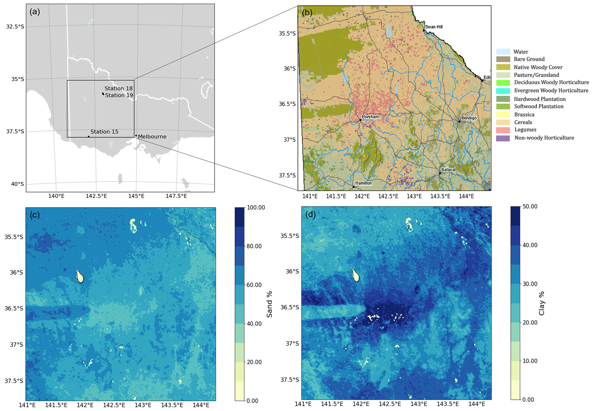
Figure 1(a) AUS-VIC simulation domain extent. (b) Dominant land use type based on VLUIS data, modified after the Victorian Government Data Directory (2018). (c) Percentage of sand content (averaged throughout the soil profile) based on SoilGrids data. (d) Percentage of clay content (averaged throughout the soil profile) based on SoilGrids. The locations of CosmOz network (Hawdon et al., 2014) stations 15 (Hamilton), 18 (Bishes), and 19 (Bennets) are indicated in panel (a).
2.1 Regional domains and surface input data
The CLM5 simulations were carried out in two regional domains, one in western Europe covering the state of North Rhine-Westphalia in Germany (DE-NRW) and one that covers large parts of the state of Victoria in Australia (AUS-VIC) (Fig. 1). The DE-NRW domain is characterized by a very diverse land cover with urban, natural and mixed agricultural areas that are mostly fed by rainwater. The agricultural land cover in DE-NRW is especially abundant in the northern and western parts of the domain along with natural vegetation and urban areas. Winter wheat, winter barley, corn, sugar beet and rape seed are the most important cash crops in DE-NRW, which are mostly rain-fed (Fig. 2, BMEL, 2020, 2022). In the southern part of the domain over the Eifel region, forests and grasslands are the dominant land cover. Recently, agricultural yield in this area was impacted in 2018 and 2019 by a late cold spell (late February to early March 2018) and extreme heat and dry spells in both summers which led to an unusually high spatial variability of yield, especially for cereals (NRW Gov., 2020; BMEL, 2020, 2022). The AUS-VIC domain covers large parts of the Australian wheat belt in the state of Victoria (Fig. 1). The land cover is dominated by rain-fed agricultural areas with large paddock sizes of mostly cereal cultivation, with winter wheat being the most important crop, followed by barley and canola (ABARES, 2020; Morse-McNabb et al., 2015), along with large patches of naturally vegetated areas (i.e. pasture, grasslands, and native woody cover) and woody horticulture and wood plantations. Unfavourable weather conditions for winter crop farming (i.e. the timing and intensity of early season rainfall events) are clearly reflected in the relatively low regional production and yield per area (ABARES, 2020).
For the DE-NRW domain, land cover information was derived from the crop and land cover dataset by Griffiths et al. (2019) that covers Germany at 30 m resolution. This dataset was generated from the Sentinel-2A MultiSpectral Instrument and the Landsat-8 Operational Land Imager (OLI) observation data from the NASA Harmonized Landsat–Sentinel dataset for the year 2016 (Claverie et al., 2018). Comparison of the derived crop type and land cover map with agricultural reference data showed a very good overall accuracy of >80 %, especially for crop types with high abundances, e.g. cereals, maize and canola (Griffiths et al., 2019). For the AUS-VIC domain, the 500 m resolution Moderate Resolution Imaging Spectroradiometer (MODIS) land cover product (Friedl and Sulla-Menashe, 2019) was aggregated to the coarser resolution of 1 km and masked with information from the latest Victorian Land Use Information System (VLUIS) product for the year 2016 (Victoria Government Data Directory, 2018; Morse-McNabb et al., 2015). The VLUIS dataset covers the whole state of Victoria and contains information on land use and land cover for each cadastral parcel. It is a product of time series analysis of remote-sensing data (MOD13Q1 or MYD13Q1 by NASA) and annually collected field data (Morse-McNabb et al., 2015).
For both domains, we used soil texture and soil organic matter information from the global SoilGrids database that provides soil information at seven depths (0, 0.05, 0.15, 0.30, 0.60, 1 and 2 m) at 250 m spatial resolution (Hengl et al., 2017). Other soil parameters, such as the saturated hydraulic conductivity and soil retention parameters, were calculated within CLM5 with the pedotransfer function after Cosby et al. (1984). Additional properties of each of the sub-grid land fractions (e.g. properties of urban land cover) were derived from the global CLM5 surface dataset (see Lawrence et al., 2018).
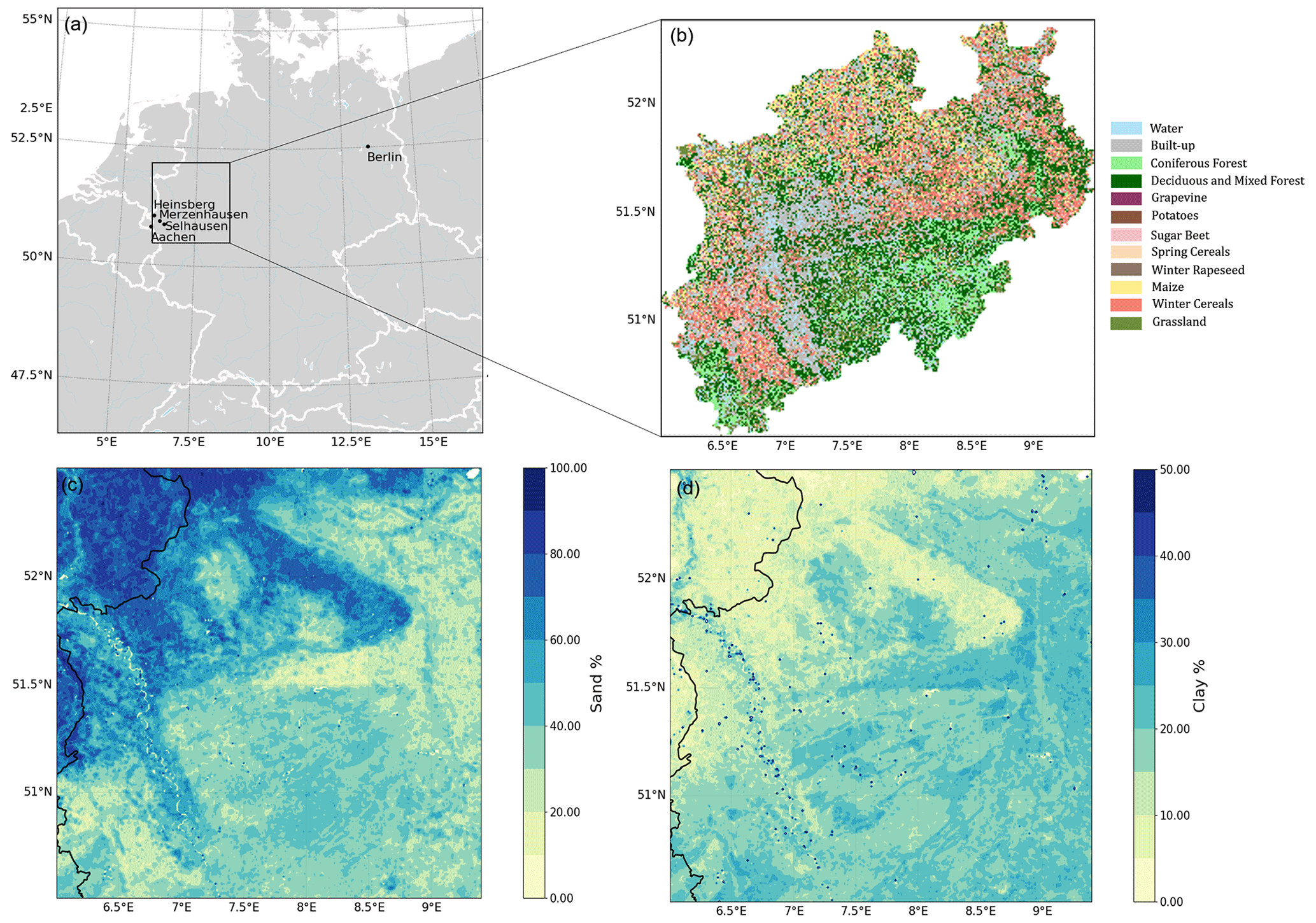
Figure 2(a) DE-NRW simulation domain extent, (b) dominant land use type based on Griffiths et al. (2018, 2019), (c) percentage of sand content (averaged throughout the soil profile) based on SoilGrids data, and (d) percentage of clay content (averaged throughout the soil profile) based on SoilGrids. The locations of the COSMOS-Europe (Bogena et al., 2022) stations Merzenhausen, Heinsberg, Selhausen, and Aachen are indicated in panel (a).
2.2 Agricultural statistics
The mild climate in Victoria is favourable to a range of winter crops, especially cereals (wheat, barley, oats), oilseeds (canola) and pulses (lentils, beans, chickpeas) contributing to Australia's total annual winter crop yield of ∼5 million tons on average. Most of the crop production in Victoria is from the western and northern regions, expanding to high-rainfall zones of southern Victoria. Wheat varieties represent the most commonly sown winter crop in Victoria, with an average operated area of 1.3 million hectares (2015 to 2019 average) (ABARES, 2020). The production of summer crops such as grain sorghum, cotton or rice in Victoria is negligible, with an average total production of 2000 t per year (2015 to 2021 average) (ABARES, 2020). The main cropping season in Victoria is from April to November. Regional average farming yield in the Victoria domain is highly influenced by seasonal rainfall patterns. In 2018, Victoria experienced substantial yield losses due to long dry spells and high temperatures after the first seasonal rainfalls, while record grain yields were recorded for the year 2020 (ABARES, 2020).
In the state of NRW, the most relevant cash crops are grain crops such as cereals (especially winter cereals) and corn, followed by canola, sugar beet and potatoes (BMEL, 2020, 2022). The main cropping season in Germany occurs during the spring and summer months until the beginning of autumn from April to the end of October. The European drought of 2018 led to local yield losses, especially for the crops corn, potatoes and sugar beet and slightly for canola, and to unusually high spatial wheat yield variability within the region. The spatial variability was strongly related to soil type (IT.NRW, 2019; NRW state government, 2020). Regions with clay-rich soils that have high water-holding capacities saw unexpectedly high wheat yields in 2019, while regions dominated by less fertile sandy soils in the north-western part of the state experienced yield losses due to water deficits (NRW state government, 2020). In general, the annual crop yield of the main cash crops varies more in Victoria than in NRW, where, on a regional average, there is only small variation between the annual yields of the respective crops (Table 2; for a complete list of cropland areas and production of major cash crops in Victoria and NRW, please see Tables S1 and S2 in the Supplement).
2.3 Land surface model
Land surface models such as CLM5 are essential tools for the study and prediction of terrestrial processes (e.g. energy, water and nutrient fluxes) and climate feedbacks in the terrestrial ecosystem and are broadly applied in different scientific disciplines (e.g. Baatz et al., 2017; Lu et al., 2017; Chang et al., 2018; Han et al., 2018; Lawrence et al., 2018, 2019; Naz et al., 2019; Lombardozzi et al., 2020). In this study, the land surface model simulations were carried out with the latest version of CLM5, which includes an adopted version of the prognostic crop module from the Agro-Ecosystem Integrated Biosphere Simulator (Kucharik and Brye, 2003; Lawrence et al., 2018). CLM5 is forced by atmospheric states at a given time step and simulates the exchange of water, energy, carbon and nitrogen between land and the atmosphere, their storage and transport on the land surface and in the sub-surface, as well as the biomass and respective yield of crops upon harvest (Lawrence et al., 2019; Lombardozzi et al., 2020). In CLM5, the plant hydraulic stress routine simulates water transport through the soil–root–stem–leaf system based on Darcy's law for porous media flow and adapts the vegetation water potential according to the water supply with transpiration demand. Water stress for plants is based on leaf water potential, which is used for the attenuation of photosynthesis in a transpiration loss function relative to maximum transpiration (Lawrence et al., 2018). The leaf stomatal conductance and leaf photosynthesis are modelled for sunlit and shaded leaves separately based on the approaches of Medlyn et al. (2011) and Farquhar et al. (1980) for C3 plants and Collatz et al. (1992) for C4 plants (Lawrence et al., 2018) respectively. Adapted from Medlyn et al. (2011), the leaf stomatal resistance is calculated using the net leaf photosynthesis, the vapour pressure deficit and the CO2 concentration at the leaf surface with plant-specific slope parameters (Lawrence et al., 2018).
With its biogeochemistry module, CLM5 is fully prognostic regarding crop phenology (e.g. grain yield, leaf area index or crop height) as well as carbon and nitrogen in the soil, vegetation and litter. The crop module includes a total of 78 plant and crop functional types, including an irrigated and non-irrigated C3 crop and crops such as winter wheat, spring wheat, canola temperate and tropical corn, temperate and tropical soybean, cotton, rice and sugarcane (Lawrence et al., 2018). Fertilization dynamics and annual fertilizer amounts in CLM5 depend on the crop functional types and vary spatially and yearly based on the land use and land cover change time series from the Land Use Model Intercomparison Project (Lawrence et al., 2016). Mineral fertilizer application starts during the leaf emergence phase of crop growth and continues for 20 d, and manure nitrogen is applied at slower rates of 0.002 kg N m−2 yr−1. For a more detailed description of the features and formulations of CLM5, the reader is referred to the technical description and the latest literature (Lawrence et al., 2018, 2019).
Here, we used a modified version of CLM5 that includes a winter cereal representation, an updated parameter set for several cash crops (winter wheat, sugar beet and potatoes) and a new sub-routine that allows the simulation of cover cropping and a more flexible crop rotation (Boas et al., 2021). The modified CLM5 version led to significantly improved simulations of LAI, net ecosystem exchange, crop yield and energy fluxes at several central European sites (Boas et al., 2021).
2.4 Seasonal weather forecasts
In this study, we used long-range meteorological forecasts from the ECMWF's fifth-generation seasonal forecasting system, SEAS5, which has been operational since November 2017 (Johnson et al., 2019). The SEAS5 forecasts are based on a coupled atmosphere–ocean model and provide forecasts of numerous meteorological variables at either 6-hourly or daily time steps at a horizontal resolution of 1∘. For the seasonal forecast, an ensemble of 51 members is initialized on the first day of a month and integrated for 7 months (Johnson et al., 2019). Furthermore, SEAS5 provides a set of retrospective seasonal hindcasts from 25 ensemble members for the years 1981 to 2016 that are used to calibrate and verify the forecasts compared to other datasets. While the whole period of hindcasts is used to verify the system, a subset from the years 1993 to 2016 is used in the calculation of forecast anomalies to avoid unreasonable effects from long-term climate trends on the forecast product (Johnson et al., 2019). A detailed description of the SEAS5 forecasting system and an overview of its performance are presented in Johnson et al. (2019). The SEAS5 forecasting product provides all the variables needed to force CLM5 at daily or 6-hourly time steps: accumulated daily precipitation amounts, daily short-wave and long-wave radiation fluxes, wind speed, air temperature, dew point temperature and mean sea level pressure. In this study, we used the years 2017 to 2020 for our simulation experiments, in accordance with the availability of the forecasting product.
We used different sets of SEAS5 forecast data, seasonal forecasts with a 7-month lead time and sub-seasonal forecasts with 3- and 4-month lead times. Those variables available at only a daily time step (incoming short-wave radiation and precipitation) were temporally disaggregated to a 6-hourly time step using the Meteorology Simulator (MetSim) (Bennett et al., 2020) to provide realistic information on atmospheric states. MetSim is based on algorithms from the Mountain Microclimate Simulation Model (MTCLIM) (Hungerford et al., 1989; Thornton and Running, 1999; Thornton et al., 2000; Bohn et al., 2013) and the Variable Infiltration Capacity (VIC) macroscale hydrologic model (Liang et al., 1994). MetSim can be used to either generate spatially distributed sub-daily time series of meteorological variables from a smaller number of input variables (daily minimum and maximum temperatures and elevation data) or to disaggregate meteorological data from a coarse temporal resolution to a finer one (Bennett et al., 2020).
In addition to the necessary meteorological input and calibration variables, MetSim also requires a grid description file that comprises information like spatial location (latitude and longitude), size of the grid cells and topography. Here, elevation data at a spatial resolution of 1 arcsec from the ASTER Global Digital Elevation Model were used (NASA/METI/AIST/Japan Spacesystem and U.S./Japan ASTER Science Team, 2019).
The daily variables were disaggregated to sub-daily resolution. The total daily precipitation was split into four equal amounts of precipitation and then spread across the sub-daily time steps (6-hourly). Similar approaches were used for the National Centre for Environmental Prediction (NCEP) dataset (Viovy, 2018) and in Hudiburg et al. (2013). Unfortunately, this deterministic approach cannot characterize the diurnal cycle of precipitation properly. The incoming short-wave radiation is disaggregated by multiplying the total daily short-wave radiation by the fraction of radiation that is calculated by the solar geometry module of MetSim. The solar geometry module within MetSim computes the daily potential radiation, day length and transmittance of the atmosphere based on the algorithms from MTCLIM (Thornton and Running, 1999). The influence of the temporal resolution of forcing data on simulation results and the quality of MetSim-disaggregated data for the CLM5 model performance relative to hourly forcing data is illustrated and discussed for an example at point scale in Appendix A1 and in the Supplement.
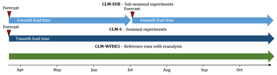
2.5 Simulation experiments
We conducted simulation experiments using different sets of seasonal (up to a 7-month lead time) and sub-seasonal (up to a 4-month lead time) forecasts in order to assess a potential difference for the prediction of annual crop yields and general model system responses for different forecast lead times. For the seasonal experiments (CLM-S), forecasts with a lead time of 7 months covering the main growing season (1 April to 31 October) were used. The seasonal simulations started on 1 April and continued for 7 months until the end of October of the same year. The same timescale was used for the sub-seasonal experiments (CLM-SUB) that were forced with a combined set of forecasts with lead times of 3 and 4 months (from 1 April until the end of June and from 1 July until 31 October) (Fig. 3). Seasonal and sub-seasonal experiments were conducted for the years 2017, 2018, 2019 and 2020 in order to assess the ability of the model to portray inter-annual differences in crop production for both domains. Furthermore, reference simulations (CLM-WFDE5) were conducted for the years 2017, 2018 and 2019 using the bias-adjusted global reanalysis dataset WFDE5 (Cucchi et al., 2020). The WFDE5 dataset was generated from the ERA5 reanalysis product (Hersbach et al., 2020) using the WATCH Forcing Data (WFD) methodology (Cucchi et al., 2020). It is provided at 0.5∘ spatial resolution and at an hourly time step for the period from 1979 to 2019.
An 850-year spin-up was performed prior to production runs for both domains in order to reach equilibrium conditions for soil carbon and nitrogen pools, soil water storage and other ecosystem variables. The global CRUNCEP atmospheric forcing dataset (Viovy, 2018) was used to force the spin-up simulations. The CRUNCEP dataset is a combination of the CRU TS3.2 0.5×0.5∘ monthly data covering the period 1901–2002 (Harris et al., 2014) and the NCEP reanalysis 2.5×2.5∘ 6-hourly data covering the period 1948–2016 (Kalnay et al., 1996).
In order to evaluate the quality of the simulation results, we used the root mean square error (RMSE), the mean bias error (MBE) and the squared correlation coefficient (R2) as statistical validation metrics:
where n is the total number of time steps; Xi and yi are the simulated and observed values of a given variable at every time step i; and the overbar represents the mean value.
2.6 Validation data
For the validation of CLM5-simulated surface soil moisture, we compared simulation results with the Soil Moisture Active Passive (SMAP) mission Enhanced Level-3 radiometer soil moisture product (SMAP L3) (Entekhabi et al., 2016) and with the Soil Moisture CCI combined dataset, version 05.2 (ESA-CCI), from the European Space Agency (ESA) Soil Moisture Essential Climate Variable (ECV) Climate Change Initiative (CCI) project (Dorigo et al., 2017; Gruber et al., 2017, 2019). The global SMAP L3 product comprises soil moisture retrievals at both 06:00 and 18:00 LT at a spatial resolution of 9 km (Entekhabi et al., 2016). The ESA-CCI soil moisture combined product provides global daily volumetric soil moisture data at a spatial resolution of 0.25∘ from 1978 to 2019. It was created by merging multiple scatterometer and radiometer soil moisture products (from the AMI-WS, ASCAT, SMMR, SSM/I, TMI, AMSR-E, WindSat, AMSR2, SMOS and SMAP satellites) and covers the period from 1978 to 2019 (Dorigo et al., 2017; Gruber et al., 2017, 2019).
In addition, simulation results were compared to available soil moisture content (SMC) measurements from three cosmic-ray neutron sensor (CRNS) measurements. For AUS-VIC we used measurement data from the stations Hamilton (station 15), Bishes (station 18) and Bennets (station 19) that are part of the CosmOz network (Hawdon et al., 2014). For DE-NRW, CRNS measurements were obtained from the four COSMOS-Europe stations Selhausen, Merzenhausen, Aachen and Heinsberg (Bogena et al., 2022). For this comparison, simulation outputs from the closest grid point to the respective station were averaged with the weighting approach after Schrön et al. (2017).
In order to validate the regional LAI and ET simulation results, we used the latest MODIS satellite data product (MCD15A3H version 6). This includes the Combined Fraction of Photosynthetically Active Radiation (FPAR) and LAI product (Myneni et al., 2015) as well as the MODIS ET/Latent Heat Flux (LH) (MOD1A2 version 6) product (Running et al., 2017). The MODIS LAI product is a 4 d composite dataset (combined acquisitions of both MODIS sensors located on NASA's Terra and Aqua satellites) on a 500 m global grid (Myneni et al., 2015). The MODIS ET product is an 8 d composite at 500 m global resolution (Running et al., 2017). We compared simulated LAI and ET with monthly mean values from MODIS for cropland-dominated land units throughout both domains.
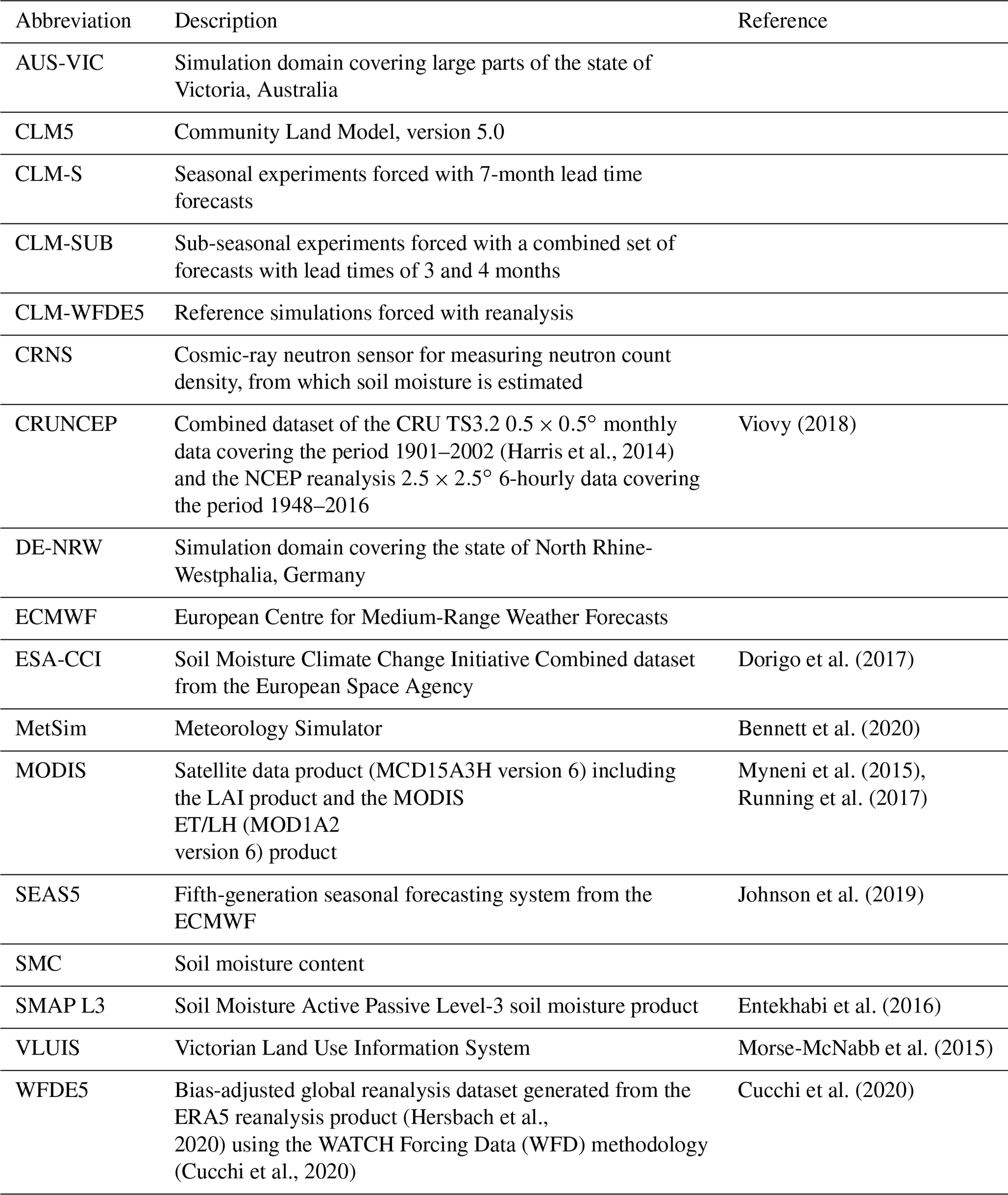
An overview of the abbreviations used in this study is provided in the Appendix (Table A1).
3.1 Comparison of seasonal forecasts to recorded weather statistics
In a first step, the forecasts for both domains were compared to official weather statistics and trends.
In 2017, the weather in Victoria was generally slightly drier and warmer than average. However, the winter season was unusually cool, with record minimum temperatures in July and August (BOM, 2021). Annual rainfall was below average in most months, especially in June and July, which resulted in the driest winter season since 2006.
However, early growing season rainfall in April was more than 50 % above average for large parts of the state (BOM, 2021). The year 2018 continued with drier and warmer-than-average weather, with the lowest annual rainfall amount since 2006 and an annual mean temperature of more than 1 ∘C above average (reference period of 1980–2010) (BOM, 2021). In the south-west and south of Victoria, winter season rainfall was close to average, while below-average rainfall amounts were recorded across the north and east of the state (BOM, 2021). Similarly to the previous years, 2019 was generally warmer and drier than average. Winter season rainfall showed high variability throughout the state: it was below average for large parts of Victoria in the north and east and above average in the south (BOM, 2021). The year 2020 continued with close-to-average rainfall and temperatures (BOM, 2021). The recorded weather pattern in Victoria is to a certain extent represented in the SEAS5 seasonal forecast data. The predicted state-wide average rainfall amount was highest for the autumn and winter seasons (from April to October) of 2020 and 2017, where recorded early season rainfall was 50 % above average, and lowest for 2018, where extremely low winter season rainfall was predicted. In NRW, the weather in 2017 was slightly warmer than the 30-year average with close-to-average rainfall. The year 2018 was characterized by an exceptional heat and drought wave during summer (Graf et al., 2020; DWD, 2021). Overall summertime rainfall in 2018 was below average, which, in combination with high temperatures, led to exceptional drought conditions in NRW and most of Europe that represent the largest annual soil moisture anomaly in the period 1979–2019 (Graf et al., 2020, and references therein). The same pattern, though less extreme, was observed in 2019, where a heat wave occurred during summer in combination with long dry spells. Total summertime rainfall was slightly below average. The year 2020 continued with above-average summertime temperatures and below-average rainfall, making it the third too dry and too warm year in a row (DWD, 2021). The trend of the recorded weather patterns is to a certain extent reflected in the SEAS5 forecasts for NRW. The predicted total rainfall over 7 months was lowest in the 2018 forecasts. The heat wave in 2018 is reflected in the forecasts of the predicted mean daily temperature, which is more than 1 ∘C higher than in 2017, 2019 and 2020.
3.2 Model performance with long-range forecasts
3.2.1 Soil moisture content
In general, the SMAP L3 dataset depicts much stronger fluctuations in the SMC than the ESA-CCI product over both domains. Over the DE-NRW domain, SMAP L3 is drier in the early growing season and shows a slightly wetter trend towards the end of the season compared to ESA-CCI (Fig. 4). Large differences in SMC can be observed for the AUS-VIC domain, where SMAP L3 shows much higher magnitudes of SMC compared to ESA-CCI, in July–September in particular. Overall, the simulated SMC shows lower fluctuations for the DE-NRW domain than for AUS-VIC. While the CLM5-simulated SMC for AUS-VIC corresponds better to the ESA-CCI product, for the DE-NRW domain, the CLM5-simulated SMC shows larger fluctuations and correlates better with the SMAP L3 product. For AUS-VIC, the CLM5-simulated SMC shows a wet trend towards the end of the winter season (August, September, October), especially for 2018 and 2019, compared to ESA-CCI (Fig. 4). The reference runs for CLM-WFDE5 generally correlated better with the ESA-CCI data (R2>0.8) than the seasonal and sub-seasonal runs (R2 values between 0.2 and 0.64) for AUS-VIC (Table 1). Overall, the fluctuations of the SMAP L3 product are not well represented in CLM5-simulated SMC over AUS-VIC. Both the forecast experiments and the reference simulations underestimated the SMC in comparison to SMAP L3 during the middle of the growing season for all the years while overestimating early and late growing season SMCs (Fig. 4).
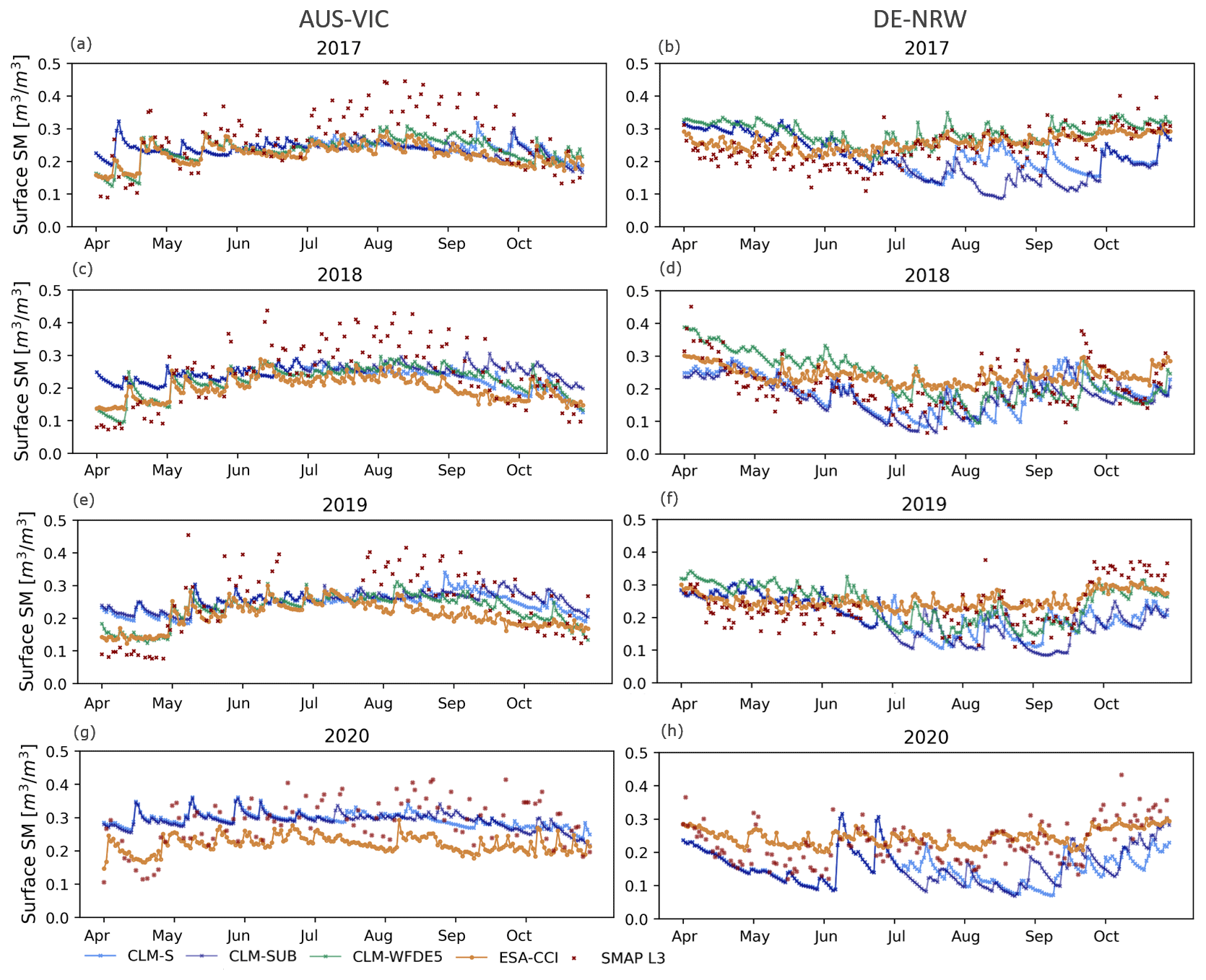
Figure 4CLM seasonal(CLM-S), sub-seasonal (CLM-SUB) and CLM-WFDE5 (for 2017, 2018 and 2019) simulated daily soil moisture content in the surface layer (0–0.05 m) from April to October 2017, 2018, 2019 and 2020 averaged over (a, c, e, g) the AUS-VIC domain and (b, d, f, h) the DE-NRW domain, compared to the ESA-CCI surface soil moisture product and SMAP L3 data for the same time period and domain respectively. Corresponding statistics (RMSE and bias) are listed in Table 1.
Table 1RMSE, MBE and R2 of CLM-S-, CLM-SUB- and CLM-WFDE5-simulated surface soil moisture (m3 m−3) (0–0.05 m) from 1 April to 31 October 2017, 2018, 2019 and 2020, compared to the ESA-CCI and SMAP L3 soil moisture products for the AUS-VIC and DE-NRW domains.
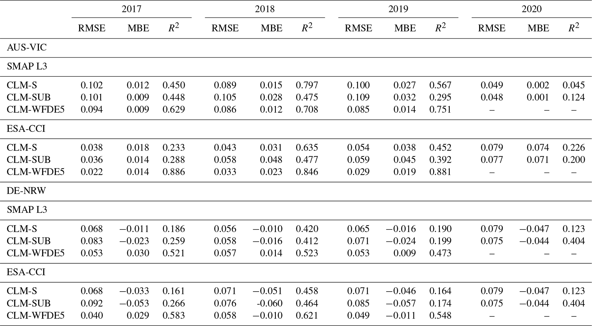
A different trend can be observed for the DE-NRW domain (Fig. 4). While simulation results from CLM-S and CLM-SUB show a slight overestimation of the surface SMC in the beginning of the growing season (April to June) of 2017 and 2019 compared to the ESA-CCI product, a clear negative bias can be observed over summer and towards the end of the growing season (July to October) of 2017 and 2020 compared to ESA-CCI (Fig. 4). This is also true for the CLM-WFDE5 run in 2018 and 2019. For 2017, CLM-WFDE5 overestimated the early season surface SMC but captured it relatively well towards the end of the season in reference to ESA-CCI (Fig. 4). Compared to the SMAP L3 product, CLM5 overestimated early growing season SMC for all the years except 2020, where a systematic underestimation of simulated SMC can be observed throughout the whole season. For the years 2018 and 2019, the SMAP L3 product seems to capture the recorded drought conditions in DE-NRW better compared to the ESA-CCI product, showing much lower SMCs. In the late growing season of 2019 (September and October), the SMAP L3 data and the ESA-CCI product show a prominent increase in SMC that is to a certain extent captured in the reference simulations but not in the seasonal and sub-seasonal experiments. Overall, the CLM-WFDE5 simulations correlated better with both SMAP L3 and ESA-CCI (R2>0.54 for all years) compared to forecast experiments (R2 values between 0.12 and 0.42).
Only minor differences between the seasonal and sub-seasonal experiments can be observed for AUS-VIC, while for DE-NRW, the sub-seasonal experiment yielded lower mean soil moisture contents compared to the seasonal model runs in the late growing season, especially in August and September of 2017.
Because of the large differences between the two validation datasets ESA-CCI and SMAP L3 over AUS-VIC, we also compared the simulated SMC to available SMC measurements from three CRNS stations (station 15: Hamilton; station 18: Bishes; station 19: Bennets) (Hawdon et al., 2014) for the years 2017 and 2018 (Fig. A2). A relatively good correlation is reached for Hamilton during the early growing seasons of 2017 and 2018, while later in the season the SMC is underestimated. The simulated SMC is relatively high at the Bennets and Bishes stations (Fig. A2) compared to CRNS data. We note that this comparison can only serve as an impression to give a tendency of model performance as simulation results and measurements may differ in soil types. For instance, Bishes and Bennets have a very sandy soil composition, while in the SoilGrids dataset the sand content is between 20 % and 40 % (Fig. 1). Station Hamilton is characterized by soils with a high water-holding capacity, which explains the high SMCs in the middle and towards the end of the wet season (Fig. A2) and which is not to the extent represented in the CLM5 simulations and underlying SoilGrids data. Single precipitation and/or flooding events that are reflected in the CRNS data are not represented in the forecasts and, thus, are naturally not captured in the simulation results. However, the reference simulations were also not able to represent these fluctuations (Fig. A2). For DE-NRW, CLM5 simulations correspond better to SMAP L3 and show more fluctuations in day-to-day SMC. Here, the forecast experiments performed reasonably well in capturing the drought conditions, with very low soil moisture contents throughout summer and autumn in 2018 and 2019. We compared CRNS measurements from four stations within DE-NRW (Selhausen, Merzenhause, Aachen and Heinsberg) (Bogena et al., 2022) to the simulated SMC at the closest grid point. The comparisons showed that the reference simulations forced with reanalysis generally produced higher SMCs than the forecast simulations and corresponded better to CRNS measurement in terms of fluctuation intensity and magnitudes than SMCs from forecast simulations for single sites (Fig. A3).
3.2.2 Leaf area index and evapotranspiration
For AUS-VIC, the simulated LAI from seasonal and sub-seasonal experiments corresponds well to MODIS data, especially for the years 2017 and 2018. Only minor differences can be observed for 2017 and 2018 between the seasonal and sub-seasonal experiments and reference simulations. For 2019, CLM-S and CLM-SUB performed better than the reanalysis run, which shows a systematic underestimation of LAI compared to MODIS throughout most of the cropping season. This is also reflected in CLM-WFDE5-simulated ET, which is strongly underestimated for 2019 compared to MODIS. CLM5 simulation results for AUS-VIC generally show a systematic negative bias in simulated ET compared to MODIS data from April to August (Fig. 5). The simulated inter-annual differences in LAI and ET are relatively small. For the DE-NRW domain, CLM5 overestimated the LAI compared to MODIS, in particular for the months June and July (Fig. 6). For 2017 and 2018, CLM-WFDE5 resulted in very similar LAI values compared to CLM-S and CLM-SUB, while for 2019 the CLM-WFDE5-simulated LAI curve peaked later (highest LAI in August) compared to forecast simulations (highest LAI in July). Both CLM-S and CLM-SUB captured lower LAI magnitudes in August 2018 compared to the other years. In general, CLM-S and CLM-SUB show only minor differences in terms of LAI and ET. An exception is the year 2017, where CLM-SUB resulted in very similar LAI values compared to MODIS in September and October while at the same time also resulting in a smaller underestimation of ET compared to CLM-S. Similarly to the results for the other domain, the simulated inter-annual differences in LAI and ET are relatively small.
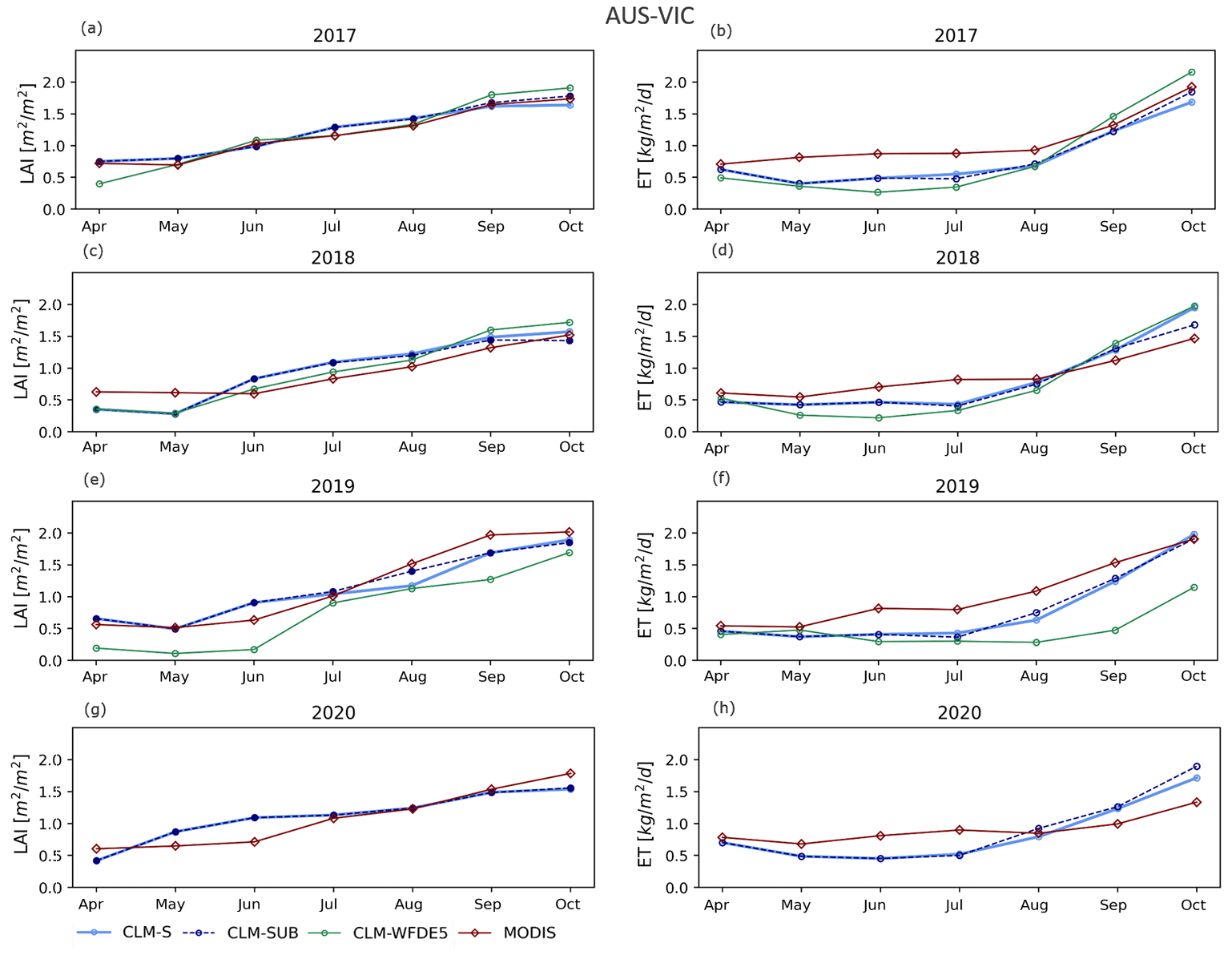
Figure 5(a, c, e, g) Monthly mean LAI and (b, d, f, h) monthly mean ET derived from MODIS for April–October 2017–2020 compared to corresponding CLM-S and CLM-SUB simulation results, averaged over all land units with more than 70 % cropland within the AUS-VIC domain.
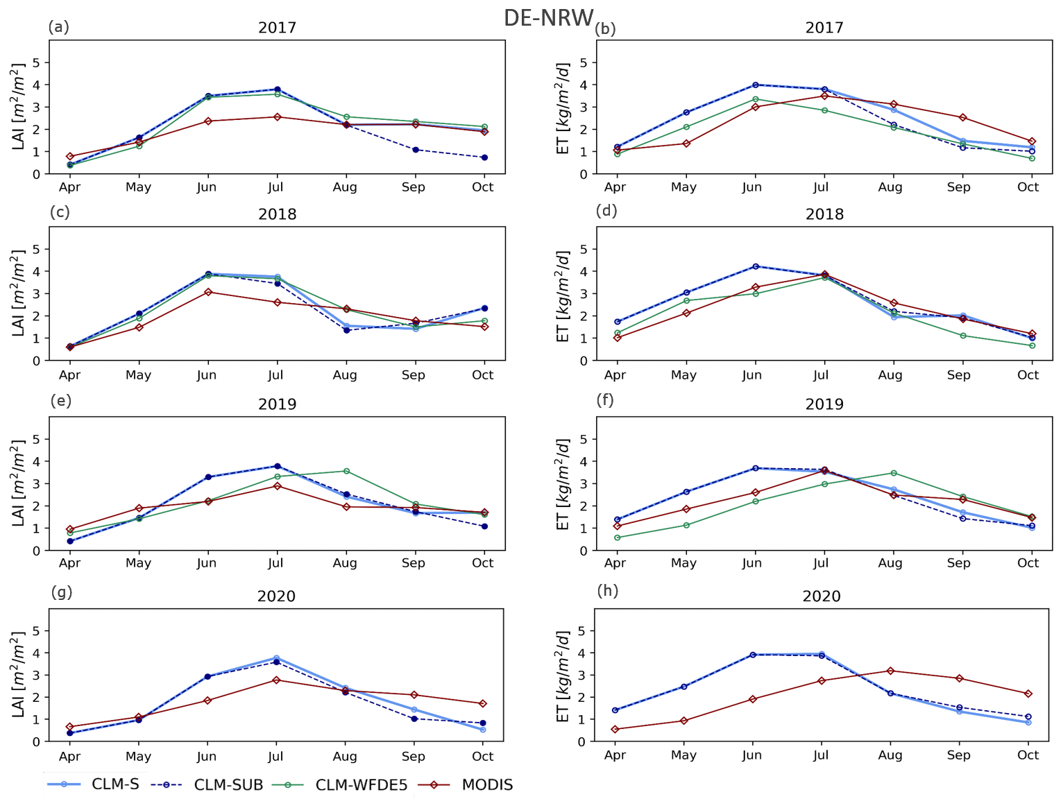
Figure 6(a, c, e, g) Monthly mean LAI and (b d, f, h) monthly mean ET derived from MODIS for April–October 2017–2020 compared to corresponding CLM-S and CLM-SUB simulation results, averaged over all land units with more than 70 % cropland within the DE-NRW domain.
3.2.3 Regional crop yield predictions
CLM5 was able to reproduce the higher annual total crop yield for the DE-NRW domain compared to AUS-VIC (Fig. 7, Table 2). For AUS-VIC, the simulations resulted in similar magnitudes of overall annual yield compared to statistics from the Australian Department of Agriculture, Water and Environment (ABARES) (Fig. 7, Table 2). CLM-S and CLM-SUB systematically underestimated the crop yield of all crops for the years 2017, 2019 and 2020 while overestimating crop yields for 2018 in comparison to official records. Still, the annual trends of recorded crop yield were to a certain extent captured in the simulations. CLM-S and CLM-SUB showed the lowest yields in 2018 and slightly higher yields in 2017, 2019 and 2020, with 2020 being the most productive year in terms of total crop yield (Fig. 7). Thus, for AUS-VIC, both the high-yield year of 2020 and the low-yield year of 2017 are well captured in the simulations. However, both the forecast experiments as well as the reference simulations resulted in a slightly lower overall yield for 2019 compared to 2017, which is contrary to the records. CLM5 simulations generally showed lower inter-annual differences in crop yield compared to the records. While the recorded annual crop yield varies by up to 50 %, simulations resulted in differences of up to 17 % for the years 2017–2020. Inter-annual differences in the mean annual crop yield (averaged for the regarded crops) of up to 1.31 t ha−1 can be observed in the records, while crop yield simulated by CLM5 showed only differences of up to 0.30 t ha−1 in the forecast simulations (0.28 t ha−1 for CLM-SUB) and up to 0.24 t ha−1 in the reference simulations. In addition, we observed a difference in the spatial distribution of crop productivity between the forecast experiments and reference simulations. While in the forecast experiments the highest crop productivity is simulated in the central and north-eastern parts of the domain, the highest crop productivity in the reference simulations is located in the southern part of the domain closer to the coastline (Fig. 8).
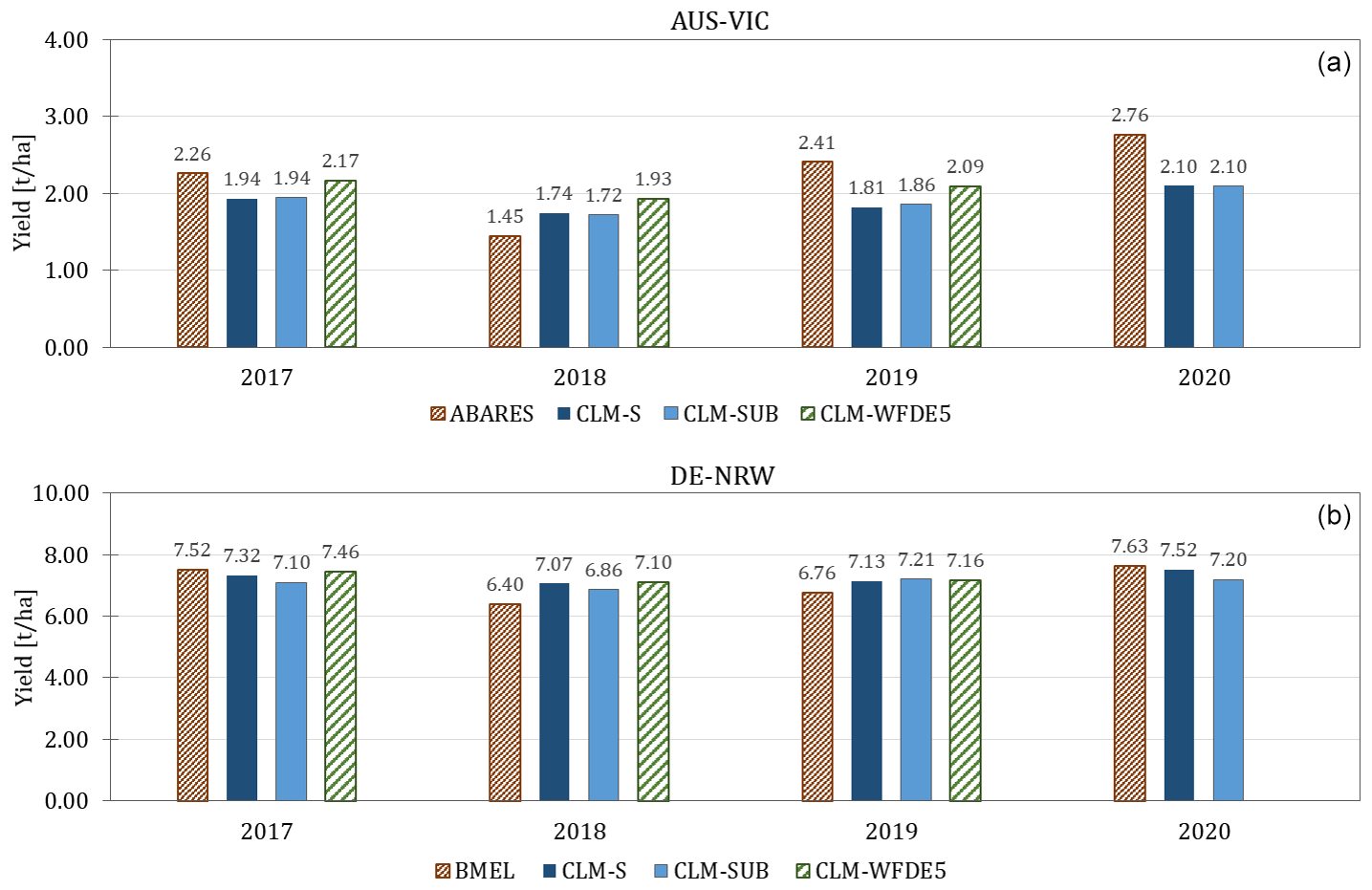
Figure 7CLM-S-, CLM-SUB- and CLM-WFDE5-simulated crop yield compared to corresponding official production records (a) from ABARES (2020), averaged for all analysed winter crops (wheat, barley and canola) within the AUS-VIC domain, and (b) from BMEL (2020, 2022), averaged for all analysed crops (wheat, corn and canola) within the DE-NRW domain, for the years 2017 to 2020. Corresponding data are listed in Table 2.
Table 2Simulated crop yields (t ha−1) for the main cash crops with CLM-S, CLM-SUB and CLM-WFDE5 forcing data for the years 2017 to 2020, compared to official crop statistics from ABARES (2020) for the AUS-VIC domain and from BMEL (2020, 2022) for the DE-NRW domain. The lowest (italics) and highest (bold) yields amongst the respective years are indicated.
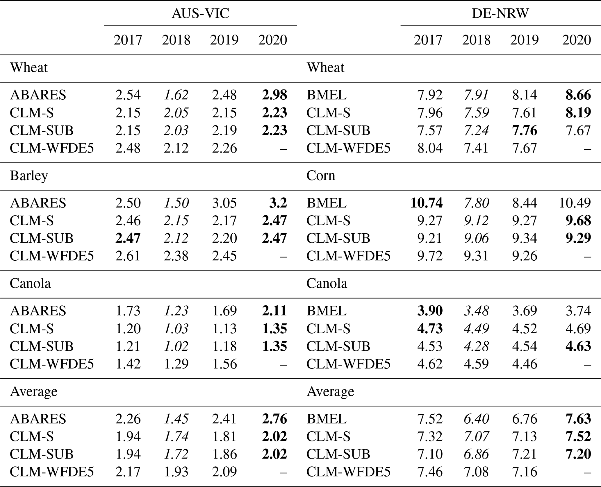
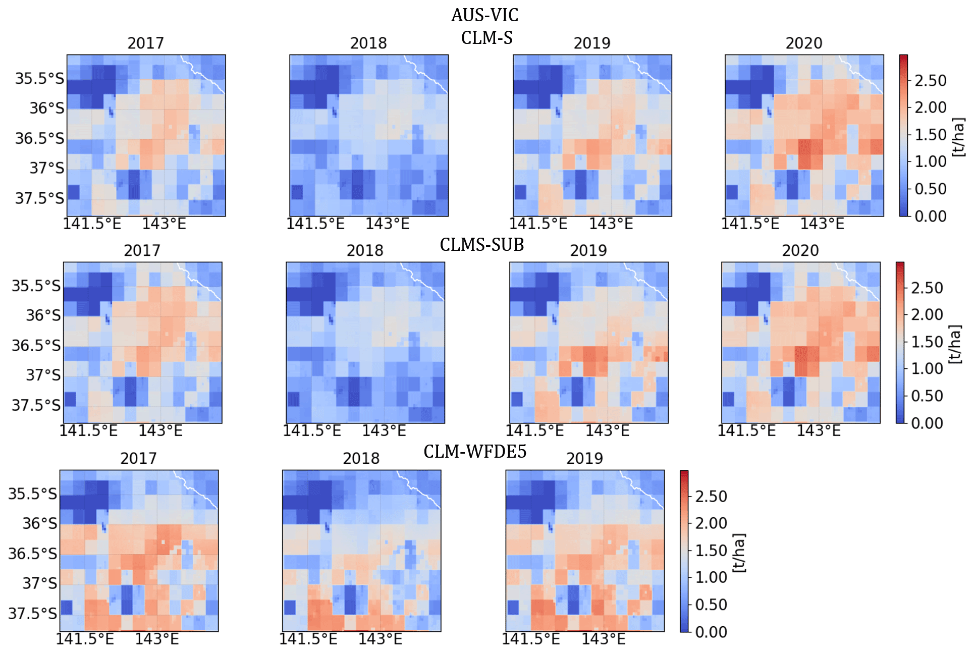
Figure 8Spatial and inter-annual differences in the simulated annual crop yield (averaged) from (top panels) CLM-S, (middle panels) CLM-SUB and (bottom panels) CLM-WFDE5 simulations throughout the AUS-VIC domain for the years 2017 to 2020.
For the DE-NRW domain, the simulated crop yields are relatively close to recorded yields in terms of magnitudes for all of the analysed cash crops wheat, corn and canola (Fig. 7, Table 2). The seasonal experiments were able to capture the high-yield year of 2020 and the yield loss in 2018. In addition, the second- and third-highest yield years are captured in CLM-S and CLM-WFDE5 simulation results but not in CLM-SUB simulation, which had higher yields in 2019 than in 2017 (Fig. 7). CLM-S performed slightly better than CLM-SUB for all years in terms of total yields compared to records, except for 2018, where the CLM-SUB yield is lower and closer to records. CLM5 simulations resulted in smaller inter-annual differences in the total annual crop yield, with up to 6 % variation compared to a recorded inter-annual difference of up to 15 % from 2017 to 2020. While inter-annual differences in crop yield of up to 1.23 t ha−1 were observed in official records, CLM5 simulations resulted in smaller differences of up to 0.45 t ha−1 in CLM-S, 0.35 t ha−1 in CLM-SUB and 0.38 t ha−1 in reference simulations on average for the regarded crops. There are no apparent spatial differences in simulated agricultural productivity between the different experiments (Fig. 9). Despite earlier enhancements to the model code and parameterization scheme (see Boas et al., 2021), the crop module of CLM5 does not include a proper representation of root crops. Here, we focus on the analysis of simulation results for wheat, corn and canola (Fig. 7). An evaluation of simulation results for root crops can be found in the Supplement (Sect. 4).
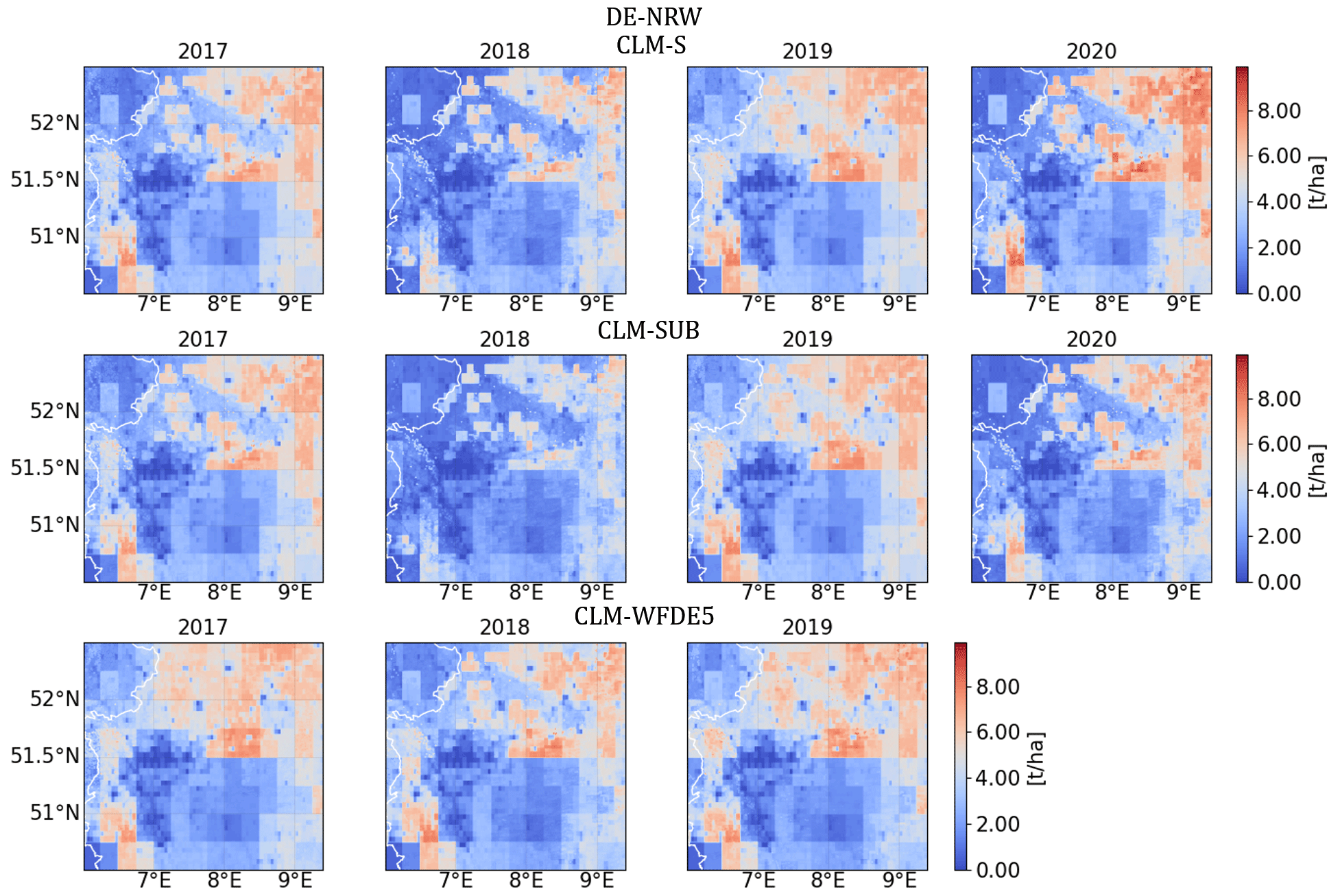
Figure 9Spatial and inter-annual differences in the simulated annual crop yield (averaged) from (top panels) CLM-S, (middle panels) CLM-SUB and (bottom panels) CLM-WFDE5 simulations throughout the DE-NRW domain for the years 2017 to 2020.
Overall, annual crop yield predictions from the forecast experiments were close to results from the reference simulations, with maximum differences between mean annual crop yield simulated with forecasts and with reanalysis of 0.28 and 0.36 t ha−1 for AUS-VIC and DE-NRW respectively. The forecast experiments were able to reproduce the recorded inter-annual trends of a high-yield year (2020) and a low-yield year (2018). In addition, the forecast experiments and the reference simulations were also able to reproduce the generally higher total values of annual crop yield for DE-NRW compared to Victoria. The lower recorded crop yields in Victoria can be explained by less productive soils, limited water availability and different crop varieties. This is to a certain extent also represented in CLM5 by a different parameterization and classification of Northern Hemisphere and Southern Hemisphere crops. Furthermore, we used the CLM5 version and parameterization that were optimized for several European cropland sites and crops in an earlier study (Boas et al., 2021). The same study revealed a significant limitation of the default CLM5 phenology module and default crop parameterization in accurately representing European cropland sites, especially in terms of crop phenology (LAI magnitudes and seasonality) and grain yield (Boas et al., 2021). Still, the inter-annual differences are lower in the CLM5 simulations compared to official yield statistics. On the one hand, this could be due to the limited resolution and quality of the forecasts that predict general meteorological trends rather than realistic weather patterns (especially for precipitation). Although seasonal and sub-seasonal forecasts correctly predicted drier and hotter trends (e.g. for 2018), the 2018 drought was less pronounced in the forecast than in the observations. In addition, we observed a difference in the spatial pattern of crop productivity over the AUS-VIC domain simulated with forecasts and reanalysis. Reference simulations resulted in a higher crop production in the southern part of the domain than forecast experiments (Fig. 8). This is related to the influence of near-coastal precipitation events that are not well represented in the forecasts.
We found that the simulated LAI and ET corresponded reasonably well to data from MODIS in terms of magnitudes and fluctuations for the AUS-VIC domain, while for the DE-NRW simulations simulated LAI and ET were larger than the observed values, in particular for the months of May, June and July. The better correlation between the simulated LAI and ET with observed values in the AUS-VIC domain, compared to DE-NRW, can be partly attributed to the larger paddock sizes and more homogeneous land cover in Victoria. The land cover in the state of NRW is more diverse, with numerous urban areas and fallow lands between croplands that are not considered to the same extent by CLM5. Moreover, agricultural management practices and the variety of crop types and cultivars are more diverse in DE-NRW, which is more challenging to represent accurately in simulations due to limitations in the input data and model structure. Several studies over European forest sites found lower absolute LAI values for MODIS compared to ground-based measurements as well as different seasonal dynamics that were partly explained by understory or herbal-layer greening together with cryptophytes and microphytes in the understory that are not included in the measurements (e.g. Wang et al., 2005; Sprintsin et al., 2009). Earlier studies with CLM5 showed relatively good correspondence between CLM5-simulated LAI and field measurements for several crops (Boas et al., 2021). For 2018, the seasonal experiments showed a relatively steep decline in LAI towards the end of the growing season that occurred earlier than for other years. The decline in LAI reflects the early simulation onset of harvest. The early harvest in a large part of the cropland in 2018 is closely linked to the recorded yield losses in NRW (Reinermann et al., 2019).
In general, the inter-annual differences in simulated LAI and ET were relatively low in the forecast experiments and in the reference simulations. This is also reflected in low inter-annual differences in simulated crop yields. The seasonal experiments were able to reproduce the generally higher inter-annual differences in crop yield throughout the AUS-VIC domain (up to 50 % in records and 17 % in simulated yields) compared to the DE-NRW domain (up to 15 % in records and 5 % in simulated yields). After weather conditions, regional agriculture and crop yield are largely impacted by agricultural management decisions (e.g. on crop varieties, planting dates, irrigation, and fertilizer types and application techniques) and other environmental factors such as pests and crop damage from wildlife, which are not sufficiently well represented by CLM5. In addition, the crop module of CLM5 lacks parameterizations for most crop types and varieties, and the fertilizer application routine is highly simplified. These deficiencies in the model structure led to considerable uncertainties in the crop phenology simulated by CLM5.
Thus, the inter-annual variability in crop yield simulated by CLM5 is primarily influenced by the variability of model forcing data and soil moisture states, as it does not consider further anthropogenic or economic factors affecting crop yield, as discussed above. Consequently, the small inter-annual differences in simulated yield suggest that the CLM5 crop module has limited sensitivity to changes in climate conditions. Uncertainties in the simulated annual crop productivity and its low inter-annual differences can be partly explained by the observed systematic biases of the simulated soil moisture content compared to satellite-derived soil moisture products, i.e. ESA-CCI and SMAP L3, and CRNS measurements for both domains.
The reference simulations showed higher correlations between the simulated and observed surface soil moisture than the forecast experiments, which could be expected given the wrong timing of precipitation events in the seasonal weather predictions while still showing similar systematic differences compared to all the products. Earlier studies with CLM3.5 (e.g. Zhao et al., 2021; Hung et al., 2022) and CLM5 (e.g. Strebel et al., 2022) found pronounced discrepancies in CLM-simulated soil moisture contents and field measurements. In this context, data assimilation has proven to be a valuable technique for reproducing better soil moisture dynamics (Strebel et al., 2022). While the assimilation of soil moisture and groundwater level data into the Terrestrial Systems Modeling Platform (TSMP), which includes an earlier version of CLM (version 3.5), significantly improved simulated soil moisture properties and groundwater levels, it had only limited effects on the resulting evapotranspiration (Hung et al., 2022). Whether a better representation of soil moisture within the model, i.e. through data assimilation, can significantly improve crop yield predictions with CLM5 remains to be evaluated.
The systematic uncertainties in the simulated soil moisture content as well as the low inter-annual differences in predicted crop yield and vegetation parameters (e.g. LAI and ET) show the need to improve the representation of these variables at the technical model level and to improve the model sensitivity to drought stress and other stressors (e.g. frost, pests, hail and wind). A sophisticated representation of crops and agricultural management in Earth system models is essential in order to better assess the impact of climate change on yield in land surface models and specifically CLM5 (Lombardozzi et al., 2020). This includes e.g. the consideration of different types of fertilizers and application strategies as well as a more detailed representation of root crops. It is crucial for the model to be sensitive enough to respond to changes in seasonality, drought stress and extreme events and realistically reflect these in resulting crop yields in order to study future yield scenarios. A better characterization of plant physiological and hydraulic properties, e.g. via plant trait information, is one suggestion for future model improvements. Studies over longer simulation periods are needed to confirm whether this low inter-annual difference in CLM5-simulated crop yield is a systematic problem.
One major challenge in applying long-range forecast products in land surface models stems from the extensive pre-processing that is needed, including the temporal downscaling of certain meteorological variables (especially incoming short-wave radiation and precipitation). Simplifications in physical model formulations and uncertainties in the forcing data (e.g. due to coarse spatial and temporal resolution) may have impacted the simulated states. A more sophisticated temporal downscaling of precipitation, e.g. through machine-learning techniques, could help improve the applicability of forecasting products for model applications and improve the quality of model system responses. This becomes especially relevant when studying the impact of extreme events on agricultural productivity and other land surface processes. However, more sophisticated downscaling approaches often require further datasets that are not readily available. A clearer statement about the SEAS5 seasonal forecasting product regarding its overall quality for land surface modelling can be made once it is available for longer timescales. A performance analysis of available hindcasts over longer timescales and for further domains could provide a further systematic evaluation of the accuracy of the products in combination with CLM5. This could also benefit the creation of appropriate tools for end-users in order to increase the user-friendliness of the respective products. For future studies, we additionally propose a benchmarking study of different forecasting products, e.g. from the German Weather Service (DWD), NCEP or CMCC Seasonal Prediction System, in combination with different land surface models like CLM5 that can point towards the relative differences and limitations of each product in terms of applicability and overall skill. We believe that such a study, in addition to providing a better representation of the current state of the art in this field, will also benefit the exchange of knowledge at the interface between science and society.
The effects of climate change and the growing demand for food production entail vulnerability and challenges for regional agriculture and food security across all scales. Reliable high-resolution seasonal weather forecasting systems can provide important information for a multitude of weather-sensitive sectors when combined with a measurable model system response.
Here, we evaluated the quality and applicability of SEAS5 long-range meteorological forecasts in combination with CLM5 for two different regions. Our analysis illustrated that simulations forced with long-range forecasts were able to generate a model system response that was close to reference simulations, which is an encouraging result for future studies. Both forecast- and reanalysis-forced models captured the inter-annual differences in yield, at least in sign (increase or decrease). The low- and high-yield seasons of 2018 and 2020 are clearly indicated for both simulated regions. The inter-annual differences in crop yield and other vegetation parameters (LAI and ET) were comparably low. Still, simulation results represented the higher inter-annual differences in crop yield across the AUS-VIC domain compared to the DE-NRW domain. While general trends of soil moisture such as the drought in 2018 were reproduced in the simulations, we found systematic overestimations and underestimations compared to different validation datasets and site observations in both the forecast and reference simulations that cannot be explained by uncertainties in the forecasting product alone. These systematic uncertainties in the simulated soil moisture and the low inter-annual differences in simulated vegetation parameters indicate the need for further technical model improvements.
Overall, this study provides a first impression of the utility and skill of the relatively new SEAS5 forecasting system for land surface models and provides an evaluation of the CLM5 crop module potential for regional-scale agricultural yield prediction in two different climate zones. Our evaluation and analysis of the CLM5 crop model performance set the stage for further model evaluation and improvements. A strong conclusion about the SEAS5 seasonal forecasting product regarding its overall quality for land surface modelling can be drawn once this is available for longer timescales. This research underlines the value of combining seasonal forecasts with land surface models such as CLM5 or similar model applications (i.e. crop models).
Table A1List of abbreviations used in this study, their descriptions and their references.
A1 Effect of temporal forcing data resolution – a synthetic experiment
In order to analyse the overall effect of temporal forcing data resolution on model outputs and to assess the general need for temporal disaggregation from daily variables for CLM5 simulations, we performed a synthetic simulation experiment for a high-resolution dataset at the point scale. We used a continuous-measurement dataset at an hourly time step for 5 consecutive years from the cropland study site Selhausen (DE-RuS) located in the western part of Germany. Selhausen (50.86589∘ N, 6.44712∘ E) is part of the TERENO (TERrestrial ENvironment Observatories) Rur Hydrological Observatory (Bogena at al., 2018), the TERENO Eifel/Lower Rhine Valley Observatory (Zacharias et al., 2011) and the Integrated Carbon Observation System (ICOS, 2020). Continuous measurements of meteorological variables and land–atmosphere exchange fluxes are available via the respective data portals (Kunkel et al., 2013; ICOS, 2020; TERENO, 2020). The original measurement data were first averaged to daily values and then temporally disaggregated to a 6-hourly time step using MetSim. Hence, simulations for a consecutive cycle of spring wheat over 5 years (hypothetical) were conducted with the reference observation data at an hourly time step, with daily averaged observations, and with the disaggregated 6-hourly forcing dataset. A spin-up was conducted prior to this trial in order to balance ecosystem carbon and nitrogen pools, gross primary production and total water storage in the system (see Lawrence et al., 2018).
As expected, the 6-hourly disaggregated data performed significantly better for all individual output variables than the daily data, which performed poorly compared to the reference forcing. The effect is especially prominent for the soil water content and the surface runoff. Here, the 6-hourly disaggregated forcing was able to capture more realistic magnitudes of both soil moisture content and runoff, resulting in only a small wet bias compared to the reference forcing (see Table S5). The 6-hourly forcing resulted in a grain yield of 4.71 t ha−1, which is relatively close to the grain yield with an hourly forcing of 4.9 t ha−1, while the simulated grain yield with a daily forcing of 4.12 t ha−1 is slightly lower. The soil moisture content (in the surface layers and the root zone) plays an important role in the simulation of reasonable crop productivity, especially when trying to simulate inter-annual differences in crop yield and crop growth in response to e.g. drought conditions. However, in the given simulation example for the DE-RuS site, water availability in the root zone does not represent the main limiting factor for plant growth for the simulated years. This explains the small variations of simulated grain yield and LAI with the different forcing datasets despite the profound differences in simulated soil water contents (Fig. A1). The results from this trial underline the importance of an adequate temporal resolution for forcing data. For the seasonal weather forecast data, the temporal disaggregation of the product to an adequate temporal resolution is crucial in order to make the data suitable for comparable model applications. A more detailed overview of this experiment and the corresponding statistics is provided in the Supplement.
A2 Comparison with CRNS data
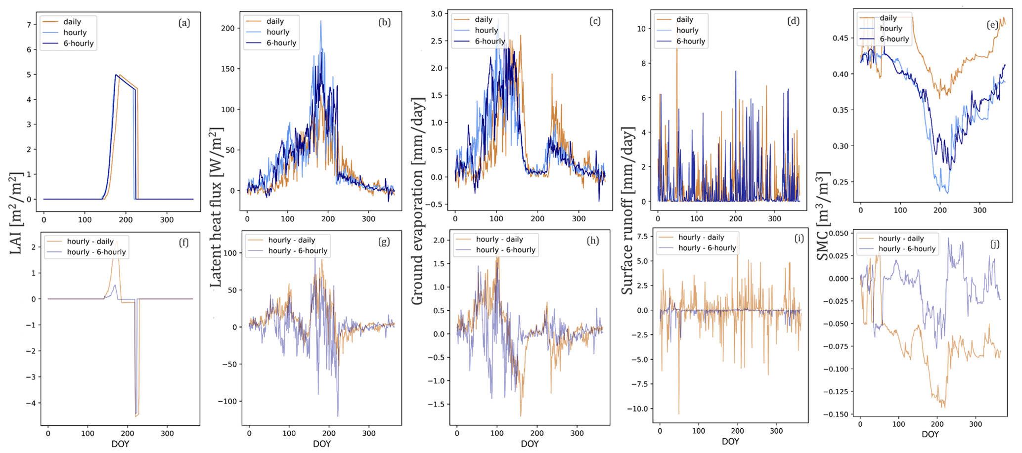
Figure A1(a–e) Comparison of simulation results for a cycle of (hypothetical) spring wheat cropping (averaged over 5 years) at DE-RuS with different temporal resolutions of the forcing data: reference simulations forced with hourly observation data (light blue), daily averaged forcing data at a 24 h time step (orange) and disaggregated forcing data at 6-hourly resolution (navy) for (a) LAI, (b) latent heat flux, (c) ground evaporation, (d) surface runoff and (e) SMC (in an upper soil layer of 0.12 to 0.20 m depth). (f–j) The difference in the simulation results for each variable. Results from the reference simulation forced with hourly data minus the daily forcing (orange) and 6-hourly disaggregated forcing (blue) respectively. Corresponding statistics are listed in Table S5.
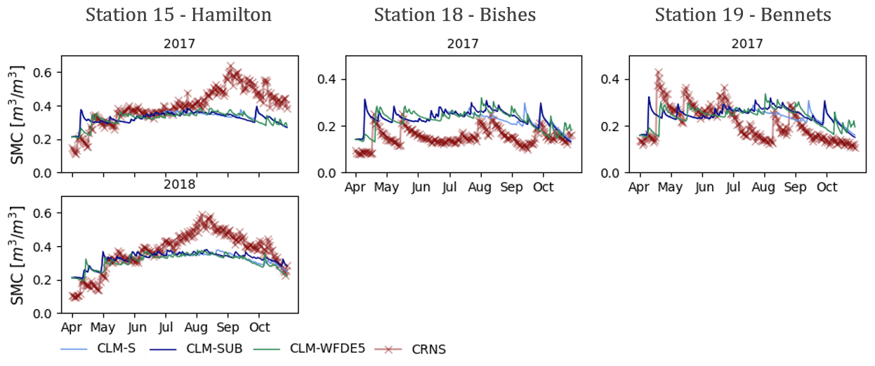
Figure A2Comparison of CRNS data (level 4) from the stations 15 (Hamilton), 18 (Bishes) and 19 (Bennets) available from the CosmOz network (Hawdon et al., 2014) with simulated SMCs at the closest grid point for the years 2017 and 2018. Corresponding statistics can be found in the Supplement.
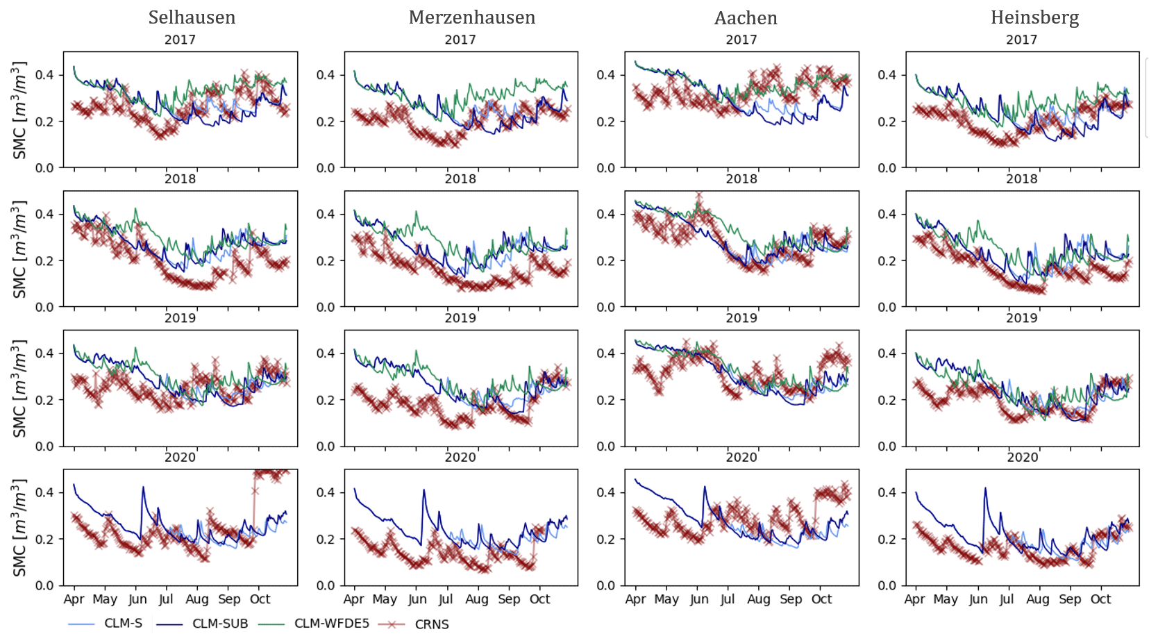
Figure A3Comparison of CRNS data from the COSMOS-Europe sites Selhausen, Merzenhausen, Aachen and Heinsberg (Bogena et al., 2022) with simulated SMCs at the closest grid point for the years 2017–2020. Corresponding statistics can be found in the Supplement.
The modified model version of CLM_WW_CC that was used in this study is publicly accessible at https://doi.org/10.5281/zenodo.3978092 (Sacks, 2020).
All underlying research data used for this study are publicly accessible. The seasonal forecast are available as daily and subdaily data on single levels via the Climate Data Store (https://doi.org/10.24381/cds.181d637e, Copernicus Climate Change Service, 2018). Soil information from SoilGrids are publicly accessible via the International Soil Reference and Information Centre (ISRIC) – World Soil Information data hub (https://www.isric.org/explore/soilgrids, ISRIC, 2023). Land cover information that was used for the DE-NRW domain can be accessed via https://doi.org/10.1594/PANGAEA.893195 (Griffiths et al., 2018). Land cover information for AUS-VIC from the Victorian Land Use Information System is publicly accessible via the Victorian Government Data Directory (2018, https://doi.org/10.4226/92/590abbe6ea3f1).
The supplement related to this article is available online at: https://doi.org/10.5194/hess-27-3143-2023-supplement.
TB conceptualized and performed the simulation experiments, curated the data, analysed and visualized the simulation results, and prepared the manuscript with contributions from all the co-authors. HB, HJHF, DR, AW and HV supervised the research and revised and edited the manuscript.
At least one of the (co-)authors is a member of the editorial board of Hydrology and Earth System Sciences. The peer-review process was guided by an independent editor, and the authors also have no other competing interests to declare.
Publisher's note: Copernicus Publications remains neutral with regard to jurisdictional claims in published maps and institutional affiliations.
The authors are grateful for the computing time granted on the supercomputer JUWLES by the Jülich Supercomputing Centre (JSC). This study is part of the Jülich-University of Melbourne Postgraduate Academy (JUMPA), an international research collaboration between the University of Melbourne, Australia, and the Research Centre Jülich, Germany.
The article processing charges for this open-access publication were covered by the Forschungszentrum Jülich.
This paper was edited by Shraddhanand Shukla and reviewed by Frank Davenport and one anonymous referee.
ABARES – Australian Bureau of Agricultural and Resource Economics and Sciences: Australian Crop Report, February 2021, Canberra, https://doi.org/10.25814/xqy3-sx57, 2020.
Ash, A., McIntosh, P., Cullen, B., Carberry, P., and Smith, M. S.: Constraints and opportunities in applying seasonal climate forecasts in agriculture, Aust. J. Agric. Res., 58, 952–965, https://doi.org/10.1071/AR06188, 2007.
Baatz, R., Hendricks Franssen, H.-J., Han, X., Hoar, T., Bogena, H. R., and Vereecken, H.: Evaluation of a cosmic-ray neutron sensor network for improved land surface model prediction, Hydrol. Earth Syst. Sci., 21, 2509–2530, https://doi.org/10.5194/hess-21-2509-2017, 2017.
Bauer, P., Thorpe, A., and Brunet, G.: The quiet revolution of numerical weather prediction, Nature, 525, 47–55, https://doi.org/10.1038/nature14956, 2015.
Bennett, A., Hamman, J., and Nijssen, B.: MetSim: A Python package for estimation and disaggregation of meteorological data, J. Open Source Softw., 5, 2042, https://doi.org/10.21105/joss.02042, 2020.
BMEL: Besondere Ernte- und Qualitätsermittlung (BEE) 2019, agricultural yield and quality assessment, https://www.bmel-statistik.de/landwirtschaft/ernte-und-qualitaet/archiv-ernte-und-qualitaet-bee (last access: 15 March 2023), 2020.
BMEL: Besondere Ernte- und Qualitätsermittlung (BEE) 2021, agricultural yield and quality assessment, https://www.bmel-statistik.de/landwirtschaft/ernte-und-qualitaet/archiv-ernte-und-qualitaet-bee (last access: 15 March 2023), 2022.
Boas, T., Bogena, H., Grünwald, T., Heinesch, B., Ryu, D., Schmidt, M., Vereecken, H., Western, A., and Hendricks Franssen, H.-J.: Improving the representation of cropland sites in the Community Land Model (CLM) version 5.0, Geosci. Model Dev., 14, 573–601, https://doi.org/10.5194/gmd-14-573-2021, 2021.
Bogena, H. R., Montzka, C., Huisman, J. A., Graf, A., Schmidt, M., Stockinger, M., von Hebel, C., Hendricks-Franssen, H. J., van der Kruk, J., Tappe, W., Lücke, A., Baatz, R., Bol, R., Groh, J., Pütz, T., Jakobi, J., Kunkel, R., Sorg, J., and Vereecken, H.: The TERENO-Rur Hydrological Observatory: A Multiscale Multi-Compartment Research Platform for the Advancement of Hydrological Science, Vadose Zone J., 17, 1–22, https://doi.org/10.2136/vzj2018.03.0055, 2018.
Bogena, H. R., Schrön, M., Jakobi, J., Ney, P., Zacharias, S., Andreasen, M., Baatz, R., Boorman, D., Duygu, M. B., Eguibar-Galán, M. A., Fersch, B., Franke, T., Geris, J., González Sanchis, M., Kerr, Y., Korf, T., Mengistu, Z., Mialon, A., Nasta, P., Nitychoruk, J., Pisinaras, V., Rasche, D., Rosolem, R., Said, H., Schattan, P., Zreda, M., Achleitner, S., Albentosa-Hernández, E., Akyürek, Z., Blume, T., del Campo, A., Canone, D., Dimitrova-Petrova, K., Evans, J. G., Ferraris, S., Frances, F., Gisolo, D., Güntner, A., Herrmann, F., Iwema, J., Jensen, K. H., Kunstmann, H., Lidón, A., Looms, M. C., Oswald, S., Panagopoulos, A., Patil, A., Power, D., Rebmann, C., Romano, N., Scheiffele, L., Seneviratne, S., Weltin, G., and Vereecken, H.: COSMOS-Europe: a European network of cosmic-ray neutron soil moisture sensors, Earth Syst. Sci. Data, 14, 1125–1151, https://doi.org/10.5194/essd-14-1125-2022, 2022.
Bohn, T. J., Livneh, B., Oyler, J. W., Running, S. W., Nijssen, B., and Lettenmaier, D. P.: Global evaluation of MTCLIM and related algorithms for forcing of ecological and hydrological models, Agr. Forest Meteorol., 176, 38–49, https://doi.org/10.1016/j.agrformet.2013.03.003, 2013.
BOM: Australian Government: Climate summaries archive, http://www.bom.gov.au/climate/current/statement_archives.shtml (last access: 10 June 2023), 2021.
Calanca, P., Bolius, D., Weigel, A. P., and Liniger, M. A.: Application of long-range weather forecasts to agricultural decision problems in Europe, J. Agric. Sci., 149, 15–22, https://doi.org/10.1017/S0021859610000729, 2011.
Cantelaube, P. and Terres, J.-M.: Seasonal weather forecasts for crop yield modelling in Europe, Tellus A, 57, 476–487, https://doi.org/10.1111/j.1600-0870.2005.00125.x, 2005.
Chang, L.-L., Dwivedi, R., Knowles, J. F., Fang, Y.-H., Niu, G.-Y., Pelletier, J. D., Rasmussen, C., Durcik, M., Barron-Gafford, G. A., and Meixner, T.: Why Do Large-Scale Land Surface Models Produce a Low Ratio of Transpiration to Evapotranspiration?, J. Geophys. Res.-Atmos., 123, 9109–9130, https://doi.org/10.1029/2018JD029159, 2018.
Claverie, M., Ju, J., Masek, J. G., Dungan, J. L., Vermote, E. F., Roger, J.-C., Skakun, S. V., and Justice, C.: The Harmonized Landsat and Sentinel-2 surface reflectance data set, Remote Sens. Environ., 219, 145–161, https://doi.org/10.1016/j.rse.2018.09.002, 2018.
Coelho, C. A. and Costa, S. M.: Challenges for integrating seasonal climate forecasts in user applications, Curr. Opin. Environ. Sustain., 2, 317–325, https://doi.org/10.1016/j.cosust.2010.09.002, 2010.
Collatz, G. J., Ribas-Carbo, M., and Berry, J. A.: Coupled Photosynthesis-Stomatal Conductance Model for Leaves of C4 Plants, Funct. Plant Biol., 19, 519–538, https://doi.org/10.1071/pp9920519, 1992.
Copernicus Climate Change Service, Climate Data Store: Seasonal forecast daily and subdaily data on single levels, Copernicus Climate Change Service (C3S) Climate Data Store (CDS) [data set], https://doi.org/10.24381/cds.181d637e, 2018.
Cosby, B. J., Hornberger, G. M., Clapp, R. B., and Ginn, T. R.: A Statistical Exploration of the Relationships of Soil Moisture Characteristics to the Physical Properties of Soils, Water Resour. Res., 20, 682–690, https://doi.org/10.1029/WR020i006p00682, 1984.
Cucchi, M., Weedon, G. P., Amici, A., Bellouin, N., Lange, S., Müller Schmied, H., Hersbach, H., and Buontempo, C.: WFDE5: bias-adjusted ERA5 reanalysis data for impact studies, Earth Syst. Sci. Data, 12, 2097–2120, https://doi.org/10.5194/essd-12-2097-2020, 2020.
Dorigo, W., Wagner, W., Albergel, C., Albrecht, F., Balsamo, G., Brocca, L., Chung, D., Ertl, M., Forkel, M., Gruber, A., Haas, E., Hamer, P. D., Hirschi, M., Ikonen, J., de Jeu, R., Kidd, R., Lahoz, W., Liu, Y. Y., Miralles, D., Mistelbauer, T., Nicolai-Shaw, N., Parinussa, R., Pratola, C., Reimer, C., van der Schalie, R., Seneviratne, S. I., Smolander, T., and Lecomte, P.: ESA CCI Soil Moisture for improved Earth system understanding: State-of-the art and future directions, Remote Sens. Environ., 203, 185–215, https://doi.org/10.1016/j.rse.2017.07.001, 2017.
DWD – Deutscher Wetter Dienst: German weather archive, https://www.dwd.de/DE/leistungen/klimadatendeutschland/klarchivtagmonat.html (last access: 15 March 2023), 2021.
Entekhabi, D., Das, N., Njoku, E., Johnson, J., and Shi, J.: SMAP L3 Radar/Radiometer Global Daily 9 km EASE-Grid Soil Moisture, Version 3, NSIDC, https://doi.org/10.5067/7KKNQ5UURM2W, 2016.
Farquhar, G. D., von Caemmerer, S., and Berry, J. A.: A biochemical model of photosynthetic CO2 assimilation in leaves of C3 species, Planta, 149, 78–90, https://doi.org/10.1007/BF00386231, 1980.
Friedl, M. and Sulla-Menashe, D.: MCD12Q1 MODIS/Terra + Aqua Land Cover Type Yearly L3 Global 500 m SIN Grid V006, NASA EOSDIS Land Processes DAAC [data set], https://doi.org/10.5067/MODIS/MCD12Q1.006, 2019.
Graf, A., Klosterhalfen, A., Arriga, N., Bernhofer, C., Bogena, H., Bornet, F., Brüggemann, N., Brümmer, C., Buchmann, N., Chi, J., Chipeaux, C., Cremonese, E., Cuntz, M., Dušek, J., El-Madany, T. S., Fares, S., Fischer, M., Foltýnová, L., Gharun, M., Ghiasi, S., Gielen, B., Gottschalk, P., Grünwald, T., Heinemann, G., Heinesch, B., Heliasz, M., Holst, J., Hörtnagl, L., Ibrom, A., Ingwersen, J., Jurasinski, G., Klatt, J., Knohl, A., Koebsch, F., Konopka, J., Korkiakoski, M., Kowalska, N., Kremer, P., Kruijt, B., Lafont, S., Léonard, J., De Ligne, A., Longdoz, B., Loustau, D., Magliulo, V., Mammarella, I., Manca, G., Mauder, M., Migliavacca, M., Mölder, M., Neirynck, J., Ney, P., Nilsson, M., Paul-Limoges, E., Peichl, M., Pitacco, A., Poyda, A., Rebmann, C., Roland, M., Sachs, T., Schmidt, M., Schrader, F., Siebicke, L., Šigut, L., Tuittila, E.-S., Varlagin, A., Vendrame, N., Vincke, C., Völksch, I., Weber, S., Wille, C., Wizemann, H.-D., Zeeman, M., and Vereecken, H.: Altered energy partitioning across terrestrial ecosystems in the European drought year 2018, Philos. T. Roy. Soc. B, 375, 20190524, https://doi.org/10.1098/rstb.2019.0524, 2020.
Griffiths, P., Nendel, C., and Hostert, P: National-scale crop- and land-cover map of Germany (2016) based on imagery acquired by Sentinel-2A MSI and Landsat-8 OLI, PANGAEA [data set], https://doi.org/10.1594/PANGAEA.893195, 2018.
Griffiths, P., Nendel, C., and Hostert, P.: Intra-annual reflectance composites from Sentinel-2 and Landsat for national-scale crop and land cover mapping, Remote Sens. Environ., 220, 135–151, https://doi.org/10.1016/j.rse.2018.10.031, 2019.
Gruber, A., Dorigo, W. A., Crow, W., and Wagner, W.: Triple Collocation-Based Merging of Satellite Soil Moisture Retrievals, IEEE T. Geosci. Remote, 55, 6780–6792, https://doi.org/10.1109/TGRS.2017.2734070, 2017.
Gruber, A., Scanlon, T., van der Schalie, R., Wagner, W., and Dorigo, W.: Evolution of the ESA CCI Soil Moisture climate data records and their underlying merging methodology, Earth Syst. Sci. Data, 11, 717–739, https://doi.org/10.5194/essd-11-717-2019, 2019.
Gubler, S., Sedlmeier, K., Bhend, J., Avalos, G., Coelho, C. A. S., Escajadillo, Y., Jacques-Coper, M., Martinez, R., Schwierz, C., Skansi, M. de, and Spirig, C.: Assessment of ECMWF SEAS5 Seasonal Forecast Performance over South America, Weather Forecast., 35, 561–584, https://doi.org/10.1175/WAF-D-19-0106.1, 2020.
Han, X., Franssen, H.-J. H., Montzka, C., and Vereecken, H.: Soil moisture and soil properties estimation in the Community Land Model with synthetic brightness temperature observations, Water Resour. Res., 6081–6105, https://doi.org/10.1002/2013WR014586@10.1002/(ISSN)1944-7973.SVASYST1, 2018.
Hansen, J. W.: Realizing the potential benefits of climate prediction to agriculture: issues, approaches, challenges, Agric. Syst., 74, 309–330, 2002.
Hansen, J. W., Challinor, A., Ines, A., Wheeler, T., and Moron, V.: Translating climate forecasts into agricultural terms: advances and challenges, Clim. Res., 33, 27–41, https://doi.org/10.3354/cr033027, 2006.
Harris, I., Jones, P. d., Osborn, T. j., and Lister, D. h.: Updated high-resolution grids of monthly climatic observations – the CRU TS3.10 Dataset, Int. J. Climatol., 34, 623–642, https://doi.org/10.1002/joc.3711, 2014.
Hawdon, A., McJannet, D., and Wallace, J.: Calibration and correction procedures for cosmic-ray neutron soil moisture probes located across Australia, Water Resour. Res., 50, 5029–5043, https://doi.org/10.1002/2013WR015138, 2014.
Hengl, T., de Jesus, J. M., Heuvelink, G. B. M., Gonzalez, M. R., Kilibarda, M., Blagotić, A., Shangguan, W., Wright, M. N., Geng, X., Bauer-Marschallinger, B., Guevara, M. A., Vargas, R., MacMillan, R. A., Batjes, N. H., Leenaars, J. G. B., Ribeiro, E., Wheeler, I., Mantel, S., and Kempen, B.: SoilGrids250m: Global gridded soil information based on machine learning, PLOS ONE, 12, e0169748, https://doi.org/10.1371/journal.pone.0169748, 2017.
Hersbach, H., Bell, B., Berrisford, P., Hirahara, S., Horányi, A., Muñoz-Sabater, J., Nicolas, J., Peubey, C., Radu, R., Schepers, D., Simmons, A., Soci, C., Abdalla, S., Abellan, X., Balsamo, G., Bechtold, P., Biavati, G., Bidlot, J., Bonavita, M., Chiara, G. D., Dahlgren, P., Dee, D., Diamantakis, M., Dragani, R., Flemming, J., Forbes, R., Fuentes, M., Geer, A., Haimberger, L., Healy, S., Hogan, R. J., Hólm, E., Janisková, M., Keeley, S., Laloyaux, P., Lopez, P., Lupu, C., Radnoti, G., de Rosnay, P., Rozum, I., Vamborg, F., Villaume, S., and Thépaut, J.-N.: The ERA5 global reanalysis, Q. J. Roy. Meteorol. Soc., 146, 1999–2049, https://doi.org/10.1002/qj.3803, 2020.
Hudiburg, T. W., Law, B. E., and Thornton, P. E.: Evaluation and improvement of the Community Land Model (CLM4) in Oregon forests, Biogeosciences, 10, 453–470, https://doi.org/10.5194/bg-10-453-2013, 2013.
Hung, C. P., Schalge, B., Baroni, G., Vereecken, H., and Hendricks Franssen, H.-J.: Assimilation of Groundwater Level and Soil Moisture Data in an Integrated Land Surface-Subsurface Model for Southwestern Germany, Water Resour. Res., 58, e2021WR031549, https://doi.org/10.1029/2021WR031549, 2022.
Hungerford, R. D., Nemani, R. R., Running, S. W., and Coughlan, J. C.: MTCLIM: a mountain microclimate simulation model, US Department of Agriculture, Forest Service, Intermountain Forest and Range Experiment Station, Ogden, UT, https://doi.org/10.2737/INT-RP-414, 1989.
ICOS: Integrated Carbon Observation System Carbon Portal, https://www.icos-cp.eu/ (last access: 15 May 2020), 2020.
International Soil Reference and Information Centre (ISRIC) – World Soil Information data hub: SoilGrids, [data set], https://www.isric.org/explore/soilgrids (last access: 10 November 2022), 2023.
IT.NRW: Ernte ausgewählter landwirtschaftlicher Feldfrüchte, yield statistics for certain cash crops, Landesbetrieb ITNRW, Düsseldorf, https://www.it.nrw/statistik/eckdaten/ernte-von-ausgewaehlten-landwirtschaftlichen-feldfruechten-und-gruenland-767 (last access: 5 August 2022), 2019.
Johnson, S. J., Stockdale, T. N., Ferranti, L., Balmaseda, M. A., Molteni, F., Magnusson, L., Tietsche, S., Decremer, D., Weisheimer, A., Balsamo, G., Keeley, S. P. E., Mogensen, K., Zuo, H., and Monge-Sanz, B. M.: SEAS5: the new ECMWF seasonal forecast system, Geosci. Model Dev., 12, 1087–1117, https://doi.org/10.5194/gmd-12-1087-2019, 2019.
Kalnay, E., Kanamitsu, M., Kistler, R., Collins, W., Deaven, D., Gandin, L., Iredell, M., Saha, S., White, G., Woollen, J., Zhu, Y., Chelliah, M., Ebisuzaki, W., Higgins, W., Janowiak, J., Mo, K.C., Ropelewski, C., Wang, J., Leetmaa, A., Reynolds, R., Jenne, R. and Joseph, D.: The NCEP/NCAR 40-Year Reanalysis Project, B. Am. Meteorol. Soc., 77, 437–447, https://doi.org/10.1175/1520-0477(1996)077<0437:TNYRP>2.0.CO;2, 1996.
Klemm, T. and McPherson, R. A.: The development of seasonal climate forecasting for agricultural producers, Agr. Forest Meteorol., 232, 384–399, https://doi.org/10.1016/j.agrformet.2016.09.005, 2017.
Kucharik, C. J. and Brye, K. R.: Integrated BIosphere Simulator (IBIS) Yield and Nitrate Loss Predictions for Wisconsin Maize Receiving Varied Amounts of Nitrogen Fertilizer, J. Environ. Qual., 32, 247–268, https://doi.org/10.2134/jeq2003.2470, 2003.
Kunkel, R., Sorg, J., Eckardt, R., Kolditz, O., Rink, K., and Vereecken, H.: TEODOOR: a distributed geodata infrastructure for terrestrial observation data, Environ. Earth Sci., 69, 507–521, https://doi.org/10.1007/s12665-013-2370-7, 2013.
Lawrence, D. M., Hurtt, G. C., Arneth, A., Brovkin, V., Calvin, K. V., Jones, A. D., Jones, C. D., Lawrence, P. J., de Noblet-Ducoudré, N., Pongratz, J., Seneviratne, S. I., and Shevliakova, E.: The Land Use Model Intercomparison Project (LUMIP) contribution to CMIP6: rationale and experimental design, Geosci. Model Dev., 9, 2973–2998, https://doi.org/10.5194/gmd-9-2973-2016, 2016.
Lawrence, D. M., Fisher, R., Koven, C., Oleson, K., Svenson, S., Vertenstein, M., Andre, B., Bonan, G., Ghimire, B., van Kampenhout, L., Kennedy, D., Kluzek, E., Knox, R., Lawrence, P., Li, F., Li, H., Lombardozzi, D., Lu, Y., Perket, J., Riley,W., Sacks,W., Shi, M.,Wieder,W., Xu, C. (lead authors), Ali, A., Badger, A., Bisht, G., Broxton, P., Brunke, M., Buzan, J., Clark, M., Craig, T., Dahlin, K., Drewniak, B., Emmons, L., Fisher, J., Flanner, M., Gentine, P., Lenaerts, J., Levis, S., Leung, L. R., Lipscomb, W., Pelletier, J., Ricciuto, D. M., Sanderson, B., Shuman, J., Slater, A., Subin, Z., Tang, J., Tawfik, A., Thomas, Q., Tilmes, S., Vitt, F., and Zeng, X.: Technical Description of version 5.0 of the Community Land Model (CLM), Natl. Cent. Atmospheric Res. (NCAR), http://www.cesm.ucar.edu/models/cesm2/land/CLM50_Tech_Note.pdf (last access: 1 June 2023), 2018.
Lawrence, D. M., Fisher, R. A., Koven, C. D., Oleson, K. W., Swenson, S. C., Bonan, G., Collier, N., Ghimire, B., Kampenhout, L. van, Kennedy, D., Kluzek, E., Lawrence, P. J., Li, F., Li, H., Lombardozzi, D., Riley, W. J., Sacks, W. J., Shi, M., Vertenstein, M., Wieder, W. R., Xu, C., Ali, A. A., Badger, A. M., Bisht, G., Broeke, M. van den, Brunke, M. A., Burns, S. P., Buzan, J., Clark, M., Craig, A., Dahlin, K., Drewniak, B., Fisher, J. B., Flanner, M., Fox, A. M., Gentine, P., Hoffman, F., Keppel‐Aleks, G., Knox, R., Kumar, S., Lenaerts, J., Leung, L. R., Lipscomb, W. H., Lu, Y., Pandey, A., Pelletier, J. D., Perket, J., Randerson, J. T., Ricciuto, D. M., Sanderson, B. M., Slater, A., Subin, Z. M., Tang, J., Thomas, R. Q., Martin, M. V., and Zeng, X.: The Community Land Model Version 5: Description of New Features, Benchmarking, and Impact of Forcing Uncertainty, J. Adv. Model. Earth Sy., 11, 4245–4287, https://doi.org/10.1029/2018MS001583, 2019.
Liang, X., Lettenmaier, D. P., Wood, E. F., and Burges, S. J.: A simple hydrologically based model of land surface water and energy fluxes for general circulation models, J. Geophys. Res.-Atmos., 99, 14415–14428, https://doi.org/10.1029/94JD00483, 1994.
Lombardozzi, D. L., Lu, Y., Lawrence, P. J., Lawrence, D. M., Swenson, S., Oleson, K. W., Wieder, W. R., and Ainsworth, E. A.: Simulating Agriculture in the Community Land Model Version 5, J. Geophys. Res.-Biogeo., 125, e2019JG005529, https://doi.org/10.1029/2019JG005529, 2020.
Lu, Y., Williams, I. N., Bagley, J. E., Torn, M. S., and Kueppers, L. M.: Representing winter wheat in the Community Land Model (version 4.5), Geosci. Model Dev., 10, 1873–1888, https://doi.org/10.5194/gmd-10-1873-2017, 2017.
Marletto, V., Ventura, F., Fontana, G., and Tomei, F.: Wheat growth simulation and yield prediction with seasonal forecasts and a numerical model, Agr. Forest Meteorol., 147, 71–79, https://doi.org/10.1016/j.agrformet.2007.07.003, 2007.
McIntosh, P. C., Pook, M. J., Risbey, J. S., Lisson, S. N., and Rebbeck, M.: Seasonal climate forecasts for agriculture: Towards better understanding and value, Field Crops Res., 104, 130–138, https://doi.org/10.1016/j.fcr.2007.03.019, 2007.
Medlyn, B. E., Duursma, R. A., Eamus, D., Ellsworth, D. S., Prentice, I. C., Barton, C. V. M., Crous, K. Y., De Angelis, P., Freeman, M., and Wingate, L.: Reconciling the optimal and empirical approaches to modelling stomatal conductance, Global Change Biol., 17, 2134–2144, https://doi.org/10.1111/j.1365-2486.2010.02375.x, 2011.
Meza, F. J., Hansen, J. W., and Osgood, D.: Economic Value of Seasonal Climate Forecasts for Agriculture: Review of Ex-Ante Assessments and Recommendations for Future Research, J. Appl. Meteorol. Clim., 47, 1269–1286, https://doi.org/10.1175/2007JAMC1540.1, 2008.
Monhart, S., Spirig, C., Bhend, J., Bogner, K., Schär, C., and Liniger, M. A.: Skill of Subseasonal Forecasts in Europe: Effect of Bias Correction and Downscaling Using Surface Observations, J. Geophys. Res.-Atmos., 123, 7999–8016, https://doi.org/10.1029/2017JD027923, 2018.
Morse-McNabb, E., Sheffield, K., Clark, R., Lewis, H., Robson, S., Cherry, D., and Williams, S.: VLUIS, a land use data product for Victoria, Australia, covering 2006 to 2013, Sci. Data, 2, 150070, https://doi.org/10.1038/sdata.2015.70, 2015.
Myneni, R., Knyazikhin, Y., and Park, T.: MOD15A2H MODIS/Terra Leaf Area Index/FPAR 8-Day L4 Global 500 m SIN Grid V006, NASA EOSDIS Land Processes DAAC, https://doi.org/10.5067/MODIS/MOD15A2H.006, 2015.
NASA/METI/AIST/Japan Spacesystems and U.S./Japan ASTER Science Team: ASTER Global Digital Elevation Model V003, https://doi.org/10.5067/ASTER/ASTGTM.003, 2019.
Naz, B. S., Kurtz, W., Montzka, C., Sharples, W., Goergen, K., Keune, J., Gao, H., Springer, A., Hendricks Franssen, H.-J., and Kollet, S.: Improving soil moisture and runoff simulations at 3 km over Europe using land surface data assimilation, Hydrol. Earth Syst. Sci., 23, 277–301, https://doi.org/10.5194/hess-23-277-2019, 2019.
Niu, G.-Y., Yang, Z.-L., Mitchell, K. E., Chen, F., Ek, M. B., Barlage, M., Kumar, A., Manning, K., Niyogi, D., Rosero, E., Tewari, M., and Xia, Y.: The community Noah land surface model with multiparameterization options (Noah-MP): 1. Model description and evaluation with local-scale measurements, J. Geophys. Res.-Atmos., 116, D12109, https://doi.org/10.1029/2010JD015139, 2011.
NRW (North Rhine-Westphalia) state government: Preliminary data on cereal grain harvest balance in 2020, https://www.land.nrw/pressemitteilung/nordrhein-westfalen-legt-erntebilanz-2020-vor, (last access: 20 June 2022), 2020.
Parton, K. A., Crean, J., and Hayman, P.: The value of seasonal climate forecasts for Australian agriculture, Agric. Syst., 174, 1–10, https://doi.org/10.1016/j.agsy.2019.04.005, 2019.
Potgieter, A. B., Schepen, A., Brider, J., and Hammer, G. L.: Lead time and skill of Australian wheat yield forecasts based on ENSO-analogue or GCM-derived seasonal climate forecasts – A comparative analysis, Agr. Forest Meteorol., 324, 109116, https://doi.org/10.1016/j.agrformet.2022.109116, 2022.
Reinermann, S., Gessner, U., Asam, S., Kuenzer, C., and Dech, S.: The Effect of Droughts on Vegetation Condition in Germany: An Analysis Based on Two Decades of Satellite Earth Observation Time Series and Crop Yield Statistics, Remote Sens., 11, 1783, https://doi.org/10.3390/rs11151783, 2019.
Running, S., Mu, Q., and Zhao, M.: MOD16A2 MODIS/Terra Net Evapotranspiration 8-Day L4 Global 500 m SIN Grid V006, USGS, https://doi.org/10.5067/MODIS/MOD16A2.006, 2017.
Sacks, B., Kluzek, E., Sobhani, N., mvertens, Levis, S., Swenson, S. C., Cheng, Y., Oleson, K., Andre, B., Hamman, J., Edwards, J., Rothstein, M., Truesdale, J., Lawrence, D., ciceconsortium, van Kampenhout, L., nanr, Koven, C., Andre, B., Fischer, R., djk2120, Wieder, W., Kauffman, B., Dunlap, R., Perket, J., Barlage, M., Serbin, S. P., and Coleman, D.: tboas/CTSM: CLM_WW_CC (reelase_08_2020), Zenodo [code], https://doi.org/10.5281/zenodo.3978092, 2020.
Schrön, M., Köhli, M., Scheiffele, L., Iwema, J., Bogena, H. R., Lv, L., Martini, E., Baroni, G., Rosolem, R., Weimar, J., Mai, J., Cuntz, M., Rebmann, C., Oswald, S. E., Dietrich, P., Schmidt, U., and Zacharias, S.: Improving calibration and validation of cosmic-ray neutron sensors in the light of spatial sensitivity, Hydrol. Earth Syst. Sci., 21, 5009–5030, https://doi.org/10.5194/hess-21-5009-2017, 2017.
Semenov, M. A. and Doblas-Reyes, F. J.: Utility of dynamical seasonal forecasts in predicting crop yield, Clim. Res., 34, 71–81, https://doi.org/10.3354/cr034071, 2007.
Sprintsin, M., Karnieli, A., Berliner, P., Rotenberg, E., Yakir, D., Cohen, S., and Rotenberg, P.: Evaluating the performance of the MODIS Leaf Area Index (LAI) product over a Mediterranean dryland planted forest, Int. J. Remote Sens., 30, 5061–5069, https://doi.org/10.1080/01431160903032885, 2009.
Strebel, L., Bogena, H. R., Vereecken, H., and Hendricks Franssen, H.-J.: Coupling the Community Land Model version 5.0 to the parallel data assimilation framework PDAF: description and applications, Geosci. Model Dev., 15, 395–411, https://doi.org/10.5194/gmd-15-395-2022, 2022.
TERENO – TERrestrial ENvironment Observatories data portal: http://www.tereno.net/ddp/ (last access: 31 December 2020), 2020.
Thornton, P. E. and Running, S. W.: An improved algorithm for estimating incident daily solar radiation from measurements of temperature, humidity, and precipitation, Agr. Forest Meteorol., 93, 211–228, https://doi.org/10.1016/S0168-1923(98)00126-9, 1999.
Thornton, P. E., Hasenauer, H., and White, M. A.: Simultaneous estimation of daily solar radiation and humidity from observed temperature and precipitation: an application over complex terrain in Austria, Agr. Forest Meteorol., 104, 255–271, https://doi.org/10.1016/S0168-1923(00)00170-2, 2000.
Troccoli, A.: Seasonal climate forecasting, Meteorol. Appl., 17, 251–268, https://doi.org/10.1002/met.184, 2010.
Trugman, A. T., Medvigy, D., Mankin, J. S., and Anderegg, W. R. L.: Soil Moisture Stress as a Major Driver of Carbon Cycle Uncertainty, Geophys. Res. Lett., 45, 6495–6503, https://doi.org/10.1029/2018GL078131, 2018.
Victorian Government Data Directory, Agriculture Victoria Research Division in the Department of Economic Development, Jobs, Transport, and Resources, Spatial Sciences Group: Victorian Land Use Information System 2016, Victorian Government Data Directory [data set], https://doi.org/10.4226/92/590abbe6ea3f1, 2018.
Viovy, N.: CRUNCEP Version 7 – Atmospheric Forcing Data for the Community Land Model, NCAR, https://doi.org/10.5065/PZ8F-F017, 2018.
Wang, B., Feng, P., Waters, C., Cleverly, J., Liu, D. L., and Yu, Q.: Quantifying the impacts of pre-occurred ENSO signals on wheat yield variation using machine learning in Australia, Agr. Forest Meteorol., 291, 108043, https://doi.org/10.1016/j.agrformet.2020.108043, 2020.
Wang, Q., Tenhunen, J., Dinh, N., Reichstein, M., Otieno, D., Granier, A., and Pilegaard, K.: Evaluation of seasonal variation of MODIS derived leaf area index at two European deciduous broadleaf forest sites, Remote Sens. Environ., 96, 475–484, https://doi.org/10.1016/j.rse.2005.04.003, 2005.
Wang, Q. J., Shao, Y., Song, Y., Schepen, A., Robertson, D. E., Ryu, D., and Pappenberger, F.: An evaluation of ECMWF SEAS5 seasonal climate forecasts for Australia using a new forecast calibration algorithm, Environ. Model. Softw., 122, 104550, https://doi.org/10.1016/j.envsoft.2019.104550, 2019.
Zacharias, S., Bogena, H., Samaniego, L., Mauder, M., Fuß, R., Pütz, T., Frenzel, M., Schwank, M., Baessler, C., Butterbach-Bahl, K., Bens, O., Borg, E., Brauer, A., Dietrich, P., Hajnsek, I., Helle, G., Kiese, R., Kunstmann, H., Klotz, S., Munch, J. C., Papen, H., Priesack, E., Schmid, H. P., Steinbrecher, R., Rosenbaum, U., Teutsch, G., and Vereecken, H.: A Network of Terrestrial Environmental Observatories in Germany, Vadose Zone J., 10, 955–973, https://doi.org/10.2136/vzj2010.0139, 2011.
Zhao, H., Montzka, C., Baatz, R., Vereecken, H., and Franssen, H.-J. H.: The Importance of Subsurface Processes in Land Surface Modeling over a Temperate Region: An Analysis with SMAP, Cosmic Ray Neutron Sensing and Triple Collocation Analysis, Remote Sens., 13, 3068, https://doi.org/10.3390/rs13163068, 2021.