Stable water isotopes and tritium tracers tell the same tale: no evidence for underestimation of catchment transit times inferred by stable isotopes in StorAge Selection (SAS)-function models

Stable isotopes (δ¹⁸O) and tritium (³H) are frequently used as tracers in environmental sciences to estimate age distributions of water. However, it has previously been argued that seasonally variable tracers, such as δ¹⁸O, generally and systematically fail to detect the tails of water age distributions and therefore substantially underestimate water ages as compared to radioactive tracers such as ³H. In this study for the Neckar River basin in central Europe and based on a >20-year record of hydrological, δ¹⁸O and ³H data, we systematically scrutinized the above postulate together with the potential role of spatial aggregation effects in exacerbating the underestimation of water ages. This was done by comparing water age distributions inferred from δ¹⁸O and ³H with a total of 21 different model implementations, including time-invariant, lumped-parameter sine-wave (SW) and convolution integral (CO) models as well as StorAge Selection (SAS)-function models (P-SAS) and integrated hydrological models in combination with SAS functions (IM-SAS).

We found that, indeed, water ages inferred from δ¹⁸O with commonly used SW and CO models are with mean transit times (MTTs) of ∼ 1–2 years substantially lower than those obtained from ³H with the same models, reaching MTTs of ∼10 years. In contrast, several implementations of P-SAS and IM-SAS models not only allowed simultaneous representations of storage variations and streamflow as well as δ¹⁸O and ³H stream signals, but water ages inferred from δ¹⁸O with these models were, with MTTs of ∼ 11–17 years, also much higher and similar to those inferred from ³H, which suggested MTTs of ∼ 11–13 years. Characterized by similar parameter posterior distributions, in particular for parameters that control water age, P-SAS and IM-SAS model implementations individually constrained with δ¹⁸O or ³H observations exhibited only limited differences in the magnitudes of water ages in different parts of the models and in the temporal variability of transit time distributions (TTDs) in response to changing wetness conditions. This suggests that both tracers lead to comparable descriptions of how water is routed through the system. These findings provide evidence that allowed us to reject the hypothesis that δ¹⁸O as a tracer generally and systematically “cannot see water older than about 4 years” and that it truncates the corresponding tails in water age distributions, leading to underestimations of water ages. Instead, our results provide evidence for a broad equivalence of δ¹⁸O and ³H as age tracers for systems characterized by MTTs of at least 15–20 years. The question to which degree aggregation of spatial heterogeneity can further adversely affect estimates of water ages remains unresolved as the lumped and distributed implementations of the IM-SAS model provided inconclusive results.

Overall, this study demonstrates that previously reported underestimations of water ages are most likely not a result of the use of δ¹⁸O or other seasonally variable tracers per se. Rather, these underestimations can largely be attributed to choices of model approaches and complexity not considering transient hydrological conditions next to tracer aspects. Given the additional vulnerability of time-invariant, lumped SW and CO model approaches in combination with δ¹⁸O to substantially underestimate water ages due to spatial aggregation and potentially other still unknown effects, we therefore advocate avoiding the use of this model type in combination with seasonally variable tracers if possible and instead adopting SAS-based models or time-variant formulations of CO models.

1 Introduction

Age distributions of water fluxes (transit time distributions, TTDs) and water stored in catchments (residence time distributions, RTDs) are fundamental descriptors of hydrological functioning (Botter et al., 2011; Sprenger et al., 2019) and catchment storage (Birkel et al., 2015). They provide a way to quantitatively describe the physical link between the hydrological response of catchments and physical transport processes of conservative solutes. While the former are largely controlled by the celerities of pressure waves propagating through the system, the latter, in contrast, occur at velocities that can be up to several orders of magnitude lower (McDonnell and Beven, 2014; Hrachowitz et al., 2016).

Water age distributions cannot be directly observed. Instead, they can, in principle, be inferred from observed tracer breakthrough curves. While practically feasible at lysimeter (e.g. Asadollahi et al., 2020; Benettin et al., 2021) and small hillslope scales (e.g. Kim et al., 2022), lack of adequate observation technology and logistical constraints make this problematic at scales larger than that. At the catchment scale, estimates of water age distributions are therefore typically inferred from models that describe the relationships between time series of observed tracer input and output signals.

Over the past decades a wide spectrum of such models has been developed. Early approaches often relied on simple lumped sine-wave (hereafter SW) or lumped-parameter convolution integral models (hereafter CO; Małoszewski and Zuber, 1982; Małoszewski et al., 1983; McGuire and McDonnell, 2006) originally developed for aquifers. In spite of their widespread application, these models feature multiple critical simplifying assumptions. Most importantly, the vast majority of these model implementations work under the assumption that water storage in catchments is at steady state and that, as a consequence, TTDs are time-invariant and can a priori be defined or calibrated. While the role of storage as a first-order control on water ages was described early in the general definition of mean turnover times (e.g. Eriksson, 1958; Bolin and Rodhe, 1973; Nir, 1973), the steady-state assumption, i.e. constant storage, may have a limited effect on TTDs in aquifers, as the fraction of transient water volumes in such systems is typically rather low. However, given the temporal variability in the hydro-meteorological system drivers (e.g. precipitation, atmospheric water demand) and the spatial heterogeneity in near-surface hydrological processes, this assumption is violated in most surface water systems worldwide and can lead to misinterpretations of the model results. This triggered the development of a more coherent framework to estimate water age distributions without the need of an a priori definition of time-invariant TTDs. Instead, probability distributions, referred to as StorAge Selection (SAS) functions, are a priori defined or calibrated, and changes in water storage are explicitly accounted for. Thus, water fluxes within and released from the system are sampled from water volumes of different ages stored in the system according to these SAS functions (Botter et al., 2011; Rinaldo et al., 2015). The general concept is firmly rooted in the development of hydro-chemical routing schemes for the Birkenes, HBV or similar models going back to at least the 1970s (e.g. Lundquist, 1977; Christophersen and Wright, 1981; Christophersen et al., 1982; Seip et al., 1985; de Groisbois et al., 1988; Hooper et al., 1988; Barnes and Bonell, 1996), as illustrated by Fig. 1 in Bergström et al. (1985). Although functionally very similar to CO model implementations that allow for transient, i.e. time-variant, TTDs (Nir, 1973; Niemi, 1977), the sampling procedure based on SAS functions has the advantage of explicitly tracking the history of water (and tracer) input to and output from the system through the water age balance. As such it explicitly accounts for non-steady state conditions, which in turn leads to the emergence of time-variant TTDs and RTDs (see the review in Benettin et al., 2022).

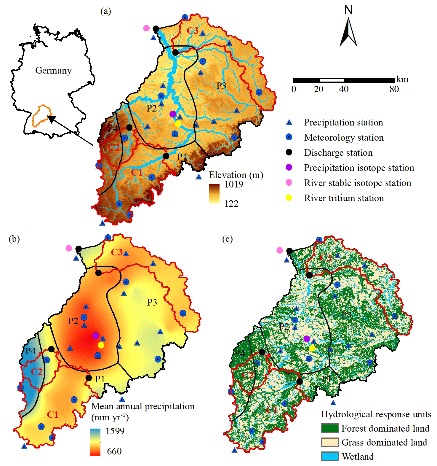
Figure 1 (a) Elevation of the Neckar catchment with discharge and hydro-meteorological stations as well as the water sampling locations used in this study. (b) The spatial distribution of long-term mean annual precipitation in the Neckar catchment and the stratification into four distinct precipitation zones P1–P4 (black outline); the red outlines indicate three sub-catchments (C1: Kirchentellinsfurt; C2: Calw; C3: Untergriesheim) within the Neckar basin. (c) Hydrological response units classified according to their land cover and topographic characteristics.

Irrespective of the modelling approach, two types of environmental tracers have in the past been frequently used to estimate water age distributions with the above models. The first type are tracers that are characterized by distinct differences in their seasonal signals. They include stable isotopes of water (²H, ¹⁸O; e.g. Małoszewski et al., 1983; Vitvar and Balderer, 1997; Fenicia et al., 2010) or solutes such as Cl⁻ (e.g. Kirchner et al., 2001, 2010; Shaw et al., 2008; Hrachowitz et al., 2009a, 2015). With these tracers, water ages and (metrics of) their distributions can be estimated by the degree to which the seasonal amplitudes of the precipitation tracer concentrations are time-shifted and/or attenuated in the streamflow (McGuire and McDonnell, 2006; Kirchner, 2016). Broadly speaking, the stronger the attenuation of the seasonally variable tracer amplitude in streamflow (A_s) as compared to its amplitude in precipitation (A_p), the older the water age can be estimated. That is, the lower the amplitude ratio $A_{\mathrm{s}}/A_{\mathrm{p}}$ is, the older the stream water is on average. The second type of commonly used tracers are radioactive isotopes such as tritium (³H). Forming the basis for many water-dating studies going back to the 1950s (e.g. Begemann and Libby, 1957; Eriksson, 1958; Dincer et al., 1970; Stewart et al., 2007; Morgenstern et al., 2010; Duvert et al., 2016; Gallart et al., 2016; Rank et al., 2018; Visser et al., 2019), water age can be estimated with radioactive tracers based on the level of radioactive decay experienced by precipitation input signals before they reach the stream.

The relationship between the tracer amplitude ratios $A_{\mathrm{s}}/A_{\mathrm{p}}$ and water age that is exploited by seasonally variable tracers is highly non-linear. With increasing attenuation of the tracer signal in the stream, i.e. a lower $A_{\mathrm{s}}/A_{\mathrm{p}}$, water therefore not only becomes older, but the age estimates also become more sensitive to changes in the amplitude ratio (Kirchner, 2016). This implies that the older the water becomes, uncertainties in the observed amplitude ratios lead to increased uncertainties in water age estimates. As a consequence, there is an upper limit to the age of water which can be practically and feasibly determined with seasonally variable tracers. A rare attempt to quantify this potential upper detectible age limit was reported by DeWalle et al. (1997). With an observed δ¹⁸O precipitation amplitude A_p=3.41 ‰, an assumed lowest possible δ¹⁸O stream water amplitude that equalled the observational error A_s=0.1 ‰, and the use of a lumped, time-invariant exponential TTD (“complete mixing”), they determined a maximum detectable MTT of around 5 years at their study site. Several authors subsequently emphasized that estimates of MTTs and in particular of maximum detectable MTTs such as reported by DeWalle et al. (1997) are specific to A_p at individual study sites (McGuire and McDonnell, 2006) and highly sensitive to choices in the modelling process (Stewart et al., 2010; Seeger and Weiler, 2014; Kirchner, 2016). For example, multiple previous studies demonstrated that the use of gamma distributions with a shape parameter α ∼0.5 as a TTD produces model results that are more consistent with observed tracer data than the use of exponential distributions (i.e. α=1) in a wide range of contrasting environments worldwide (Kirchner et al., 2001; Godsey et al., 2010; Hrachowitz et al., 2010a, b). Merely replacing the exponential distribution by a gamma distribution with α=0.5 as a TTD at the study site of DeWalle et al. (1997) leads, in a quick back-of-the-envelope calculation, to a substantial increase in the maximum MTT from the reported 5 years to ∼90 years. This is exacerbated by the potential presence of spatial aggregation bias in the lumped implementation of that model, which may cause further considerable underestimation of an MTT as demonstrated by Kirchner (2016).

The relevance of the above assumptions is often overlooked and, in spite of little additional quantitative evidence, it remains widely assumed that water ages in systems characterized by MTTs > 4–5 years cannot be meaningfully quantified with seasonally variable tracers. Most notably, Stewart et al. (2010, 2012) argued that water older than that remains hidden to stable water isotopes and other seasonally variable tracers, which inevitably results in a misleading truncation of water age distributions. Such a pronounced and systematic underestimation of water ages would have far-reaching consequences for estimates of water storage (e.g. Birkel et al., 2015; Pfister et al., 2017) and the associated turnover times of nutrients and contaminants in catchments (e.g. Harman, 2015; Hrachowitz et al., 2015). Stewart et al. (2012) further argue that the use of radioactive tracers, such as ³H, can largely avoid the truncation of the long tails of TTDs. This is mostly due to the ³H half-life of $T_{\mathrm{1}/\mathrm{2}}=\mathrm{12.32}$ years. Even with the current atmospheric ³H concentrations that, after peaking in the early 1960s, have been converging back towards pre-nuclear bomb-testing levels, precipitation ³H signals can be detected in the system for several decades, making ³H an effective tracer now and for the foreseeable future (Michel et al., 2015; Harms et al., 2016; Stewart and Morgenstern, 2016). Indeed, a range of studies based on ³H and often in conjunction with lumped-parameter convolution integral approaches suggests that many catchments and larger river basins worldwide are characterized by MTTs that are decadal or higher (e.g. Stewart et al., 2010, and references therein). It is further rather remarkable that such elevated water ages are largely absent in estimates derived from lumped-parameter convolution integral studies based on seasonally variable tracers, which often indicate MTTs between 1 and 3 years (e.g. McGuire and McDonnell, 2006, and references therein; Hrachowitz et al., 2009b; Godsey et al., 2010), as correctly and importantly pointed out by Stewart et al. (2010). This in itself could be supporting evidence for the failure of seasonally variable tracers to detect long tails of TTDs, as postulated by Stewart et al. (2012). However, it could just as well be a mere artifact arising from a sample bias due to the different catchments analysed or from choices in the modelling process. There are only a few studies that have directly and systematically compared estimates of water age derived from both seasonally variable (²H, ¹⁸O) and radioactive tracers (³H) at the same study site and based on (at least partly) comparable model approaches (Małoszewski et al., 1983; Uhlenbrook et al., 2002; Stewart et al., 2007; Stewart and Thomas, 2008). The MTT estimates derived from seasonally variable tracers in these comparative studies are consistently but to varying degrees lower than estimates based on ³H. However, these studies are nevertheless subject to limitations that may weaken the generality of the conclusion that seasonally variable tracers underestimate catchment water ages. More specifically, tracer data were available for only rather short time periods of about 2–3 years, including, for some studies, only a handful of ³H data points. Many of these studies relied on lumped-parameter convolution integral approaches with time-invariant TTDs whose pre-defined functional form when applied with seasonally variable tracers was limited to shapes (e.g. exponential) that already a priori precluded the representation of heavy tails and thus a meaningful representation of old ages. In addition, the models to estimate water ages in these studies were implemented in a spatially lumped way, which further exacerbates the potential for underestimating water ages due to spatial aggregation effects in environments that are likely subject to considerable heterogeneity in hydrological functioning (Kirchner, 2016).

Addressing some of the concerns above, a recent study by Rodriguez et al. (2021) compared catchment water ages inferred from 2-year data records of a seasonally variable tracer (²H; 1088 data points) and ³H (24 data points) using a spatially lumped implementation of a previously developed simple tracer circulation model based on the SAS approach that generates time-variant TTDs (Rodriguez and Klaus, 2019). In spite of consistently higher age estimates obtained from ³H, the absolute differences from ²H-inferred estimates were very minor. While the difference in mean transit times was estimated at ΔMTT ∼0.22 years for MTTs ∼3 years, the difference in the estimate of the 90th percentile of water ages, as a metric for the presence of old ages, was with Δ90th ∼0.15 years even lower. The authors concluded that these results cast some doubt on “[…] the perception that stable isotopes systematically truncate the tails of TTDs” (Rodriguez et al., 2021). However, their interpretation was questioned by Stewart et al. (2021), who pointed out that older water may simply not be present in their study catchment.

Building on the above work of Rodriguez et al. (2021), the objective of this study is therefore to further scrutinize the notion that the use of seasonally variable tracers leads to truncated estimates of water age distributions in a systematic comparative experiment. The novel aspects of this study for the ∼ 13 000 km² Neckar River basin in south-western Germany include the facts that, here, we use (1) long-term records, i.e. >20 years, of hydrological data as well as of seasonally variable (¹⁸O) and radioactive tracers (³H) together with (2) a suite of lumped and spatially semi-distributed implementations of (3) SW, CO and SAS-function-based models, including a formulation of an integrated, process-based model to simultaneously reproduce hydrological and tracer response dynamics and to track temporally variable water age distributions in the system. The above points allow us to, at least partially, explore several unresolved questions about how different factors may or may not contribute to the apparent underestimation of water ages by seasonally variable tracers, including potential effects of uncertainties arising from short data records, spatial aggregation and the use of oversimplified time-invariant, lumped models. More specifically, here we test the hypothesis that ¹⁸O as a tracer generally and systematically cannot detect tails in water age distributions and that this truncation leads to systematically younger water age estimates than the use of ³H.

2 Study site

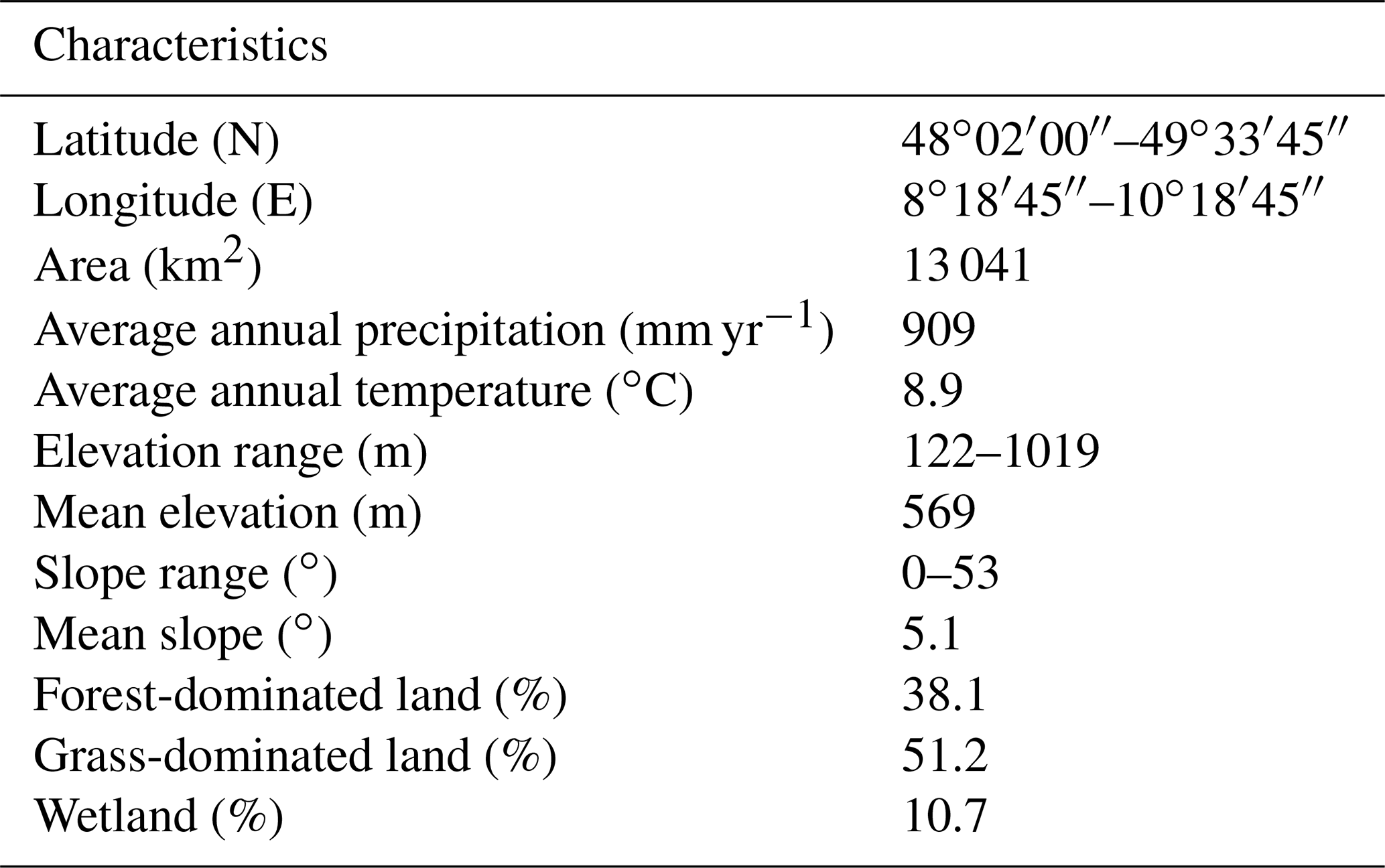
The Neckar River basin in south-western Germany has an area of ∼ 13 000 km². The elevation in the basin ranges from 122 m at the outlet in the north to about 1019 m in the south (Fig. 1a; Table 1). Following the elevation gradient, the landscape is characterized by terrace-like elements and undulating hills with wide valleys used as grasslands and croplands in the lower regions, in particular in the northern parts of the Neckar basin, and increasingly steep and narrow forested valleys towards the southern parts (Fig. 1c). Long-term mean annual precipitation (P) reaches ∼909 mm yr⁻¹, with considerable spatial variability ranging from ∼660 mm yr⁻¹ in the lower parts of the basin to over 1500 mm yr⁻¹ at high elevations in the south-west (Fig. 1b). With a long-term mean temperature of about 8.9 ^∘C, potential evaporation (E_P) around ∼870 mm yr⁻¹ and an aridity index (I_A) (i.e. $I_{\mathrm{A}}=E_{\mathrm{P}}/P$) of I_A∼0.98, the basin is characterized by a temperate–humid climate where snow cover can be present for several weeks in the winter months.

Table 1 Characteristics of the Neckar catchment in Germany.

3 Data

3.1 Data

Daily hydro-meteorological data were available for the period 1 January 1970–31 December 2016. As the forcing data of the hydrological models, daily precipitation and daily mean air temperature were obtained from stations operated by the German Weather Service (DWD). Precipitation was recorded at 16 stations and temperature measurements were available at 12 stations (Fig. 1) in or close to the study basin. Daily mean discharge data for the period 1 January 1970–31 December 2016 at the outlet of the Neckar basin at Rockenau station were provided by the German Federal Institute of Hydrology (BfG). In addition, data of daily mean discharge for the same time period from three sub-catchments within the Neckar basin (Fig. 1) at the gauges Kirchentellinsfurt (C1; 2324 km²), Calw (C2; 584 km²) and Untergriesheim (C3; 1827 km²) were available from the Environmental Agency of the Baden-Württemberg region (LUBW).

Long-term volume-weighted monthly δ¹⁸O data in precipitation were available for the period 1 January 1978–31 December 2016 at the Stuttgart station. At the sampling gauge, a monthly accumulation bottle was filled with the collected daily precipitation, and all collected water was mixed together. Therefore, the water samples of precipitation reflect the volume-weighted monthly isotopic composition. Then, a monthly isotope sample bottle for a stable isotope (i.e. ¹⁸O) was filled with 50 mL precipitation water from the corresponding monthly accumulation bottle. All the precipitation samples were tightly sealed and stored in a dark room at ∼4 ^∘C before analysis. Monthly stream water samples were collected at Schwabenheim, close to the Rockenau discharge station, by the BfG for the period of 1 October 2001–31 December 2016 (Schmidt et al., 2020; Königer et al., 2022). Note that the available data do not represent instantaneous grab samples but bulk samples from mixed daily samples. River water was sampled automatically by samplers (SP III-XY-36, Maxx Meb- und Probenahmetechnik GmbH, Germany) that contained 36 bottles (each with a volume of 2.5 L). Every 30 min, 50 mL of river water was pumped into one bottle (48 subsamples per day). A new bottle was filled every 24 h with the same procedure. All daily river water samples were stored in the sample compartment at ∼4 ^∘C and were subsequently combined into monthly samples in the laboratory of the BfG. This means that the stream water samples reflect a non-flow-weighted monthly average isotopic composition. The stable isotope ratios were analysed with dual-inlet mass spectrometry and a laser-based cavity ring-down spectrometer (L2120-i/L2130-i, Picarro Inc.) at the Helmholtz Zentrum München, Germany. When changing from dual-inlet mass spectrometry to cavity ring-down spectrometry, the long-term precision of the analytical systems (±0.15 ‰ and ±0.1 ‰, respectively, for δ¹⁸O) was ensured (Stumpp et al., 2014; Reckerth et al., 2017).

Long-term monthly ³H data in precipitation were obtained for the period 1 January 1978–31 December 2016 at the Stuttgart station (the same station as for ¹⁸O data in precipitation; Schmidt et al., 2020). For the purpose of establishing robust initial conditions for the model experiment (see Sect. 4.2), the tritium record in precipitation was reconstructed for the preceding 1970–1977 period by bias-correcting data from the sampling station Vienna that are available from the Global Network of Isotopes in Precipitation, which is a joint database of the International Atomic Energy Agency (IAEA) and the World Metrological Organization (WMO) (Fig. S1 in the Supplement). The precipitation for tritium data was sampled based on the same method as that for ¹⁸O in precipitation, which means that the precipitation samples for tritium also reflect the volume-weighted monthly isotopic composition. Stream water samples for tritium were collected based on the same method as that for ¹⁸O in streams. Therefore, tritium stream water samples also reflect non-volume-weighted monthly average isotopic compositions. The tritium stream water samples are not influenced by water release from nuclear power stations. All the water samples were analysed for tritium concentrations by the BfG Environmental Radioactivity Laboratory using liquid scintillation counters (Ultima Gold LLT) with a 2σ analytical uncertainty (Schmidt et al., 2020).

Land use types of the catchments are determined using the CORINE Land Cover data set of 2018 (https://land.copernicus.eu/pan-european/corine-land-cover). The 90 m × 90 m digital elevation model of the study region (Fig. 1a) was obtained from https://www.usgs.gov/, last access: 14 August 2023 and used to derive the local topographic indices, including height above nearest drainage (HAND) and slope.

3.2 Data pre-processing

For the subsequent model experiment (Sect. 4.2), the study basin was stratified into four regions P1–P4 that are characterized by a distinct long-term precipitation pattern (hereafter precipitation zones). In the following the procedure to infer these precipitation zones and to estimate the associated differences in δ¹⁸O and ³H input is described.

3.2.1 Spatial distribution of precipitation and identification of precipitation zones

To account, at least to some degree, for spatial heterogeneity in precipitation, we stratified the Neckar River basin into precipitation zones that are each characterized by distinct average annual precipitation totals. Goovaerts (2000) and Lloyd (2005) showed that areal precipitation estimates informed by elevation data were often more accurate than those based on precipitation gauge observations alone. Thus, to interpolate and estimate areal precipitation across the basin, we used co-kriging considering elevation, as a preliminary analysis suggested lower errors. Finally, the individual precipitation estimates for each grid cell were used with K-means clustering to establish four clusters representing the four precipitation zones P1–P4 (see Fig. 1b).

3.2.2 Spatial extrapolation of precipitation δ¹⁸O to precipitation zones

Records of observed precipitation δ¹⁸O are available at one location close to the centre of the Neckar basin (Fig. 1). However, it is well described (e.g. Kendall and Mcdonnell, 2012) that precipitation δ¹⁸O input can be subject to considerable spatial heterogeneity largely controlled by topographic and meteorological influences. Stumpp et al. (2014) specifically identified latitude, elevation and temperature as the key factors controlling δ¹⁸O input heterogeneity in the greater study region. To at least partially account for these effects and to locally adjust δ¹⁸O input signals throughout the study basin, we made use of the sinusoidal isoscapes method (Allen et al., 2018, 2019). Briefly, this method exploits the seasonal pattern in δ¹⁸O precipitation signals by fitting sine functions to observed δ¹⁸O input signals for a large sample of locations:

$$\begin{array}{}\text{(1)}& {{\mathit{\delta }}^{\mathrm{18}}\mathrm{O}}_{\mathrm{P}}\left(t\right)=a_{\mathrm{P}}\sin \left(\mathrm{2}\mathit{\pi }t-{\mathit{\phi }}_{\mathrm{P}}\right)+b_{\mathrm{P}},\end{array}$$

with a_P (‰) the amplitude of the seasonal precipitation signal, b_P (‰) a constant offset and φ_P (rad) the phase of the signal. For each of the three fitting parameters, i.e. a_P, b_P and φ_P, multiple regression relationships were previously developed (Allen et al., 2018). Depending on the fitting parameter, predictor variables included a selection of latitude, longitude, elevation, range of annual temperature and mean annual precipitation (Allen et al., 2018). The relationships defined by these predictor variables then allow one to estimate a_P, b_P and φ_P and thus the seasonal signal of ${{\mathit{\delta }}^{\mathrm{18}}\mathrm{O}}_{\mathrm{P}}$ for locations where no precipitation δ¹⁸O observations are available.

Here, we adopted the method as described in the following. In a first step, we estimated the sine-wave parameters for the time series of precipitation δ¹⁸O observed at the Stuttgart station, using the procedure described by Allen et al. (2018). Subsequently, we estimated the associated sine-wave parameters a_P, b_P and φ_P in each of the four precipitation zones (P1–P4; Table S2 in the Supplement) based on Eqs. (S1)–(S3) in the Supplement, using the above-described individual predictor variables averaged for each precipitation zone (Table S1 in the Supplement). We then used the estimated sine-wave parameters to construct an individual δ¹⁸O_P sine wave for each precipitation zone (Eq. 1). In a last step, we adjusted the observed δ¹⁸O input for the four precipitation zones by rescaling and bias-correcting the observed δ¹⁸O signal according to the differences between the sine waves at the observation station and sine waves estimated for each precipitation zone, respectively (Fig. S2 in the Supplement).

3.2.3 Spatial extrapolation of precipitation ³H to precipitation zones

As for δ¹⁸O, it is well documented that ³H exhibits spatial heterogeneity that is to some extent controlled by geographical factors. It has been shown that the ³H concentration in precipitation increases with latitude, with the highest concentrations in polar regions (Rozanski et al., 1991). In addition, ³H concentrations in precipitation increase with elevation due to the ³H-enriched upper troposphere and isotopic exchange between liquid water and atmospheric moisture, depleting ³H in lower-tropospheric layers (Tadros et al., 2014). Considering the above effects, we established a multiple linear regression relationship between ³H concentrations in precipitation observed at 15 multiple locations across Germany (Fig. S3 in the Supplement) as available through the WISER database (IAEA and WMO, 2022; Schmidt et al., 2020) together with their corresponding elevations and latitudes, respectively (Fig. S4 in the Supplement). We then used this relationship to adjust the ³H precipitation input for the four precipitation zones according to their corresponding average latitude and elevation estimate:

$$\begin{array}{}\text{(2)}& {}^{\mathrm{3}}{\mathrm{H}}_{\mathrm{P}}\left(t\right)=-\mathrm{0.75}\left(L_{\mathrm{P}}-L_{\mathrm{o}}\right)-\mathrm{0.002}\left(E_{\mathrm{P}}-E_{\mathrm{o}}\right){+}^{\mathrm{3}}{H}_{\mathrm{o}},\end{array}$$

where ³H_P is the latitude- and elevation-adjusted tritium precipitation concentration for each precipitation zone (P1–P4); ³H_o is the tritium precipitation concentration observed at the Stuttgart station; L_P and E_P are the mean latitude and elevation, respectively, of each precipitation zone; and L_o and E_o are the latitude and elevation, respectively, of the Stuttgart station.

4 Methods

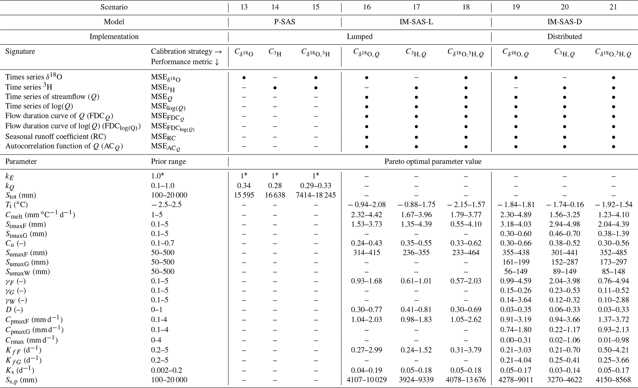
The experiment to test the hypothesis that the use of δ¹⁸O data systematically leads to truncated water age distributions and associated underestimations of water ages is designed and executed in a step-wise approach: 21 different scenarios of model types and spatial implementations thereof are sequentially calibrated and tested to reproduce observed δ¹⁸O and ³H signals in streamflow. For each of these models, several metrics of water age distributions resulting from the two independent calibration procedures, i.e. for δ¹⁸O and ³H, respectively, are then estimated and compared. As a baseline and to ensure comparability with previous studies, water ages are quantified with spatially lumped, time-invariant implementations of 12 commonly used SW and CO model scenarios (Table 2): sine-wave models using exponential (SW-EM) and gamma distributions as TTDs (SW-GM; only δ¹⁸O), lumped-parameter convolution integral models using exponential (CO-EM) and gamma distributions as TTDs (CO-GM), two-parallel reservoirs (CO-2EM), three-parallel reservoirs (CO-3EM) as well as an exponential piston flow (CO-EPM) implementation. The above baseline scenarios are complemented by nine additional models on the basis of SAS functions (Table 3). In order of increasing complexity, these include three spatially integrated formulations of a “pure” SAS-function approach with one storage component and based on observed streamflow (P-SAS), three implementations of a spatially integrated hydrological model with tracer routing based on SAS functions (IM-SAS-L) as well as three spatially distributed implementations of the same integrated hydrological model in combination with SAS functions (IM-SAS-D).

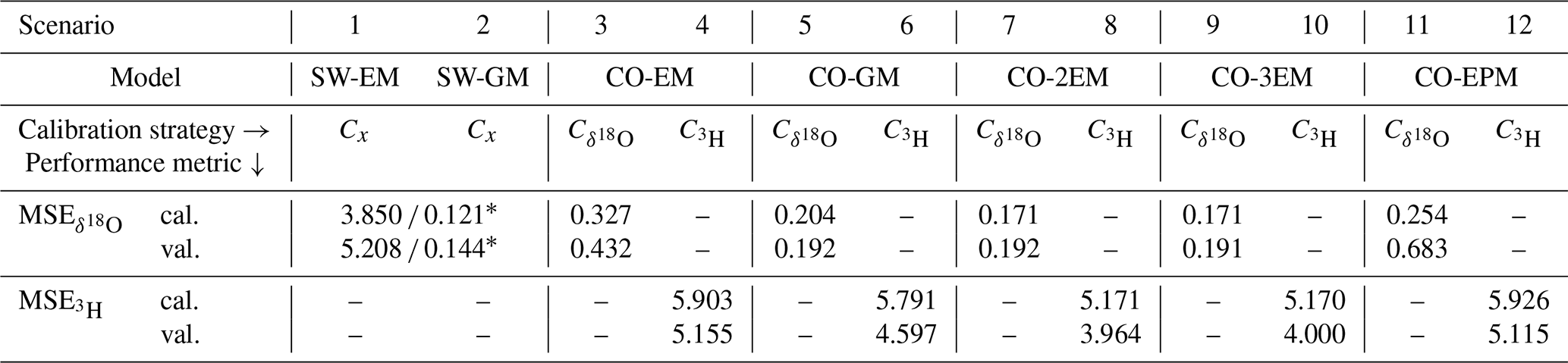
Table 2 The 12 time-invariant, lumped sine-wave (SW) and lumped-parameter convolution integral (CO) model scenarios implemented here for the Neckar study basin together with the associated calibration strategies, the individual calibration performance metric, the types of models, the prior parameter ranges and the optimal parameter value from calibration. EM represents an exponential TTD and GM indicates a gamma distribution TTD. 2EM indicates a two-parallel linear reservoir model, 3EM indicates a three-parallel linear reservoir model, and EPM indicates an exponential piston flow model. The calibration strategies show which variable a model was calibrated to using the mean square error (MSE) with $C_{{\mathit{\delta }}^{\mathrm{18}}\mathrm{O}}$ calibration to the observed stream water δ¹⁸O signal and $C_{{}^{\mathrm{3}}\mathrm{H}}$ calibration to observed stream water ³H. ^a Note that, for SW models, calibration involves least-square fits of sine waves to both the precipitation and streamflow signals available. ^b Fixed to a value of 1.

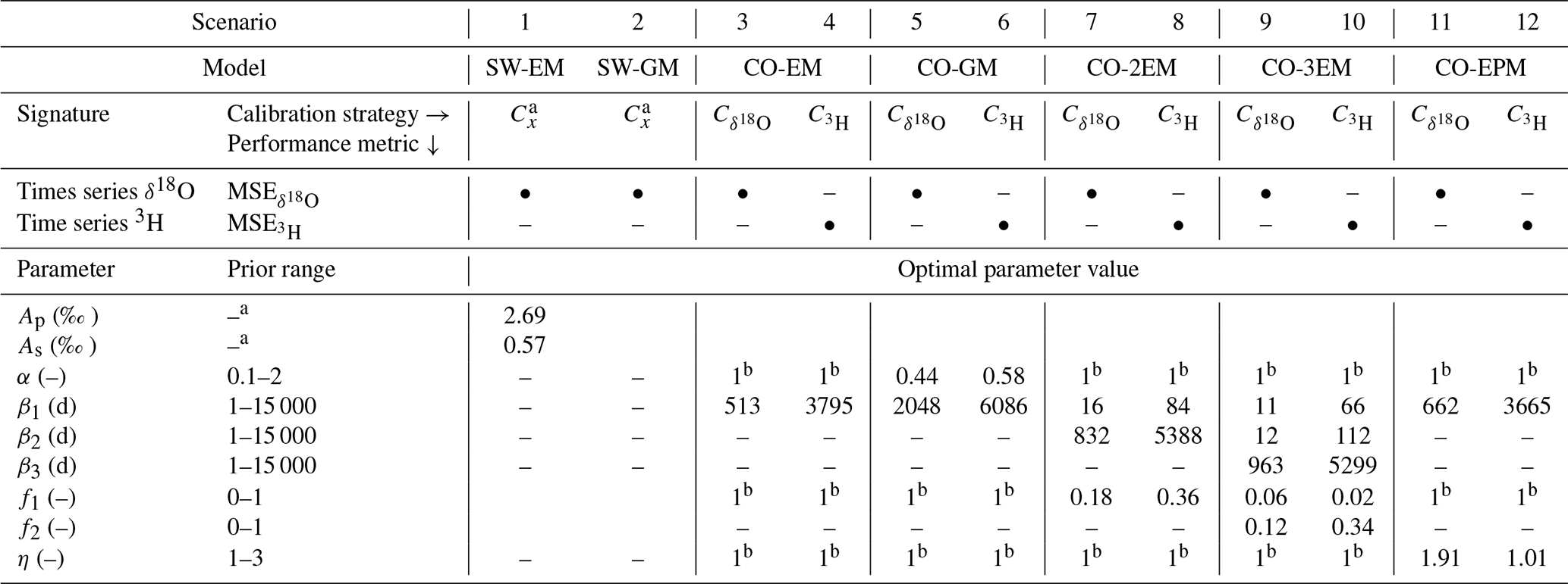
Table 3 The nine P-SAS and IM-SAS model scenarios implemented here for the Neckar study basin together with the associated calibration strategies, the individual calibration performance metrics, the type of spatial implementation (lumped or distributed) and the associated prior parameter ranges and ranges of the Pareto optimal solutions from calibration. P-SAS indicates the model with one compartment as described in Benettin et al. (2017), and IM-SAS indicates the integrated hydrological model based on SAS functions. The symbols L and D indicate lumped and distributed model implementations, respectively. The calibration strategies show which variables and signatures a model was simultaneously calibrated to using the MSE with $C_{{\mathit{\delta }}^{\mathrm{18}}\mathrm{O},Q}$ simultaneous calibration to δ¹⁸O and six signatures of streamflow Q; $C_{{}^{\mathrm{3}}\mathrm{H},Q}$ simultaneous calibration to ³H and the signatures of Q; and $C_{{\mathit{\delta }}^{\mathrm{18}}\mathrm{O},{}^{\mathrm{3}}\mathrm{H},Q}$ simultaneous calibration to δ¹⁸O, ³H and the signatures of Q. ^* Fixed to a value of 1.

4.1 Models

4.1.1 SW model

As demonstrated by Małoszewski et al. (1983), sine waves fitted to δ¹⁸O precipitation and streamflow signals can be used to indicatively determine water ages. More specifically, the ratio of the amplitudes of the fitted sine waves, i.e. $A_{\mathrm{s}}/A_{\mathrm{p}}$, can be used together with the assumption of a shape of the TTD to estimate the associated MTT of a system. In the case of a gamma distribution as a TTD, this is done according to (Kirchner, 2016)

$$\begin{array}{}\text{(3)}& \stackrel{\mathrm{‾}}{\mathit{\tau }}=\mathit{\alpha }\mathit{\beta },\end{array}$$

with

$$\begin{array}{}\text{(4)}& \mathit{\beta }={\displaystyle \frac{\mathrm{1}}{\mathrm{2}\mathit{\pi }f}}\sqrt{{\left(A_{\mathrm{s}}/A_{\mathrm{p}}\right)}^{-\mathrm{2}/\mathit{\alpha }}-\mathrm{1}},\end{array}$$

where $\stackrel{\mathrm{‾}}{\mathit{\tau }}$ is the MTT, α is a shape parameter, β is a scale parameter, and f here is the frequency for the seasonal δ¹⁸O signal, i.e. f=1 yr⁻¹. Here we analyse the two cases α=1 (SW-EM) and 0.5 (SW-GM). Note that, with α=1, the gamma distribution is equivalent to an exponential distribution. The sine-wave model is a simplification of a convolution integral model and can be directly derived from that. For a more detailed description of the method and underlying assumptions, we refer the reader to McGuire and McDonnell (2006) and Kirchner (2016).

4.1.2 Time-invariant, lumped-parameter (CO) model

While the sine-wave approach requires regular cyclic signals of tracer composition, i.e. sine waves fitted to the observations, convolution integral models make direct use of the observed tracer data (e.g. Kreft and Zuber, 1978). Tracer composition in the system output can thus be estimated based on a convolution operation of the tracer composition in the system input together with an a priori assumption of a TTD (e.g. Małoszewski and Zuber, 1982; Kirchner et al., 2001):

$$\begin{array}{}\text{(5)}& C_{\mathrm{o}}\left(t\right)={\int }_{\mathrm{0}}^{\mathrm{\infty }}g\left(\mathit{\tau }\right)C_{\mathrm{i}}\left(t-\mathit{\tau }\right)e^{-\mathit{\lambda }\mathit{\tau }}\mathrm{d}\mathit{\tau },\end{array}$$

where C_o(t) is the tracer composition of the system output (here streamflow) at time t; C_i(t−τ) is the tracer composition of the system input (here precipitation) at any previous time t−τ; λ is the radioactive decay constant (λ=0.00015 d⁻¹ for ³H and λ=0 d⁻¹ for stable isotopes); and g(τ) is the distribution of transit times τ. Here, we used gamma distributions as a basis for a flexible and general formulation of TTDs in the different CO scenarios tested in this study:

$$\begin{array}{}\text{(6)}& \begin{array}{rl}& g\left(\mathit{\tau }\right)={\sum }_{i=\mathrm{1}}^N\mathit{\eta }{f}_i{\displaystyle \frac{{\mathit{\tau }}^{\mathit{\alpha }-\mathrm{1}}}{{\mathit{\beta }}_i^{\mathit{\alpha }}\mathrm{\Gamma }\left(\mathit{\alpha }\right)}}{e}^{\left(\frac{-\mathit{\tau }}{\mathit{\eta }{\mathit{\beta }}_i}+\frac{\mathrm{1}}{\mathit{\eta }}-\mathrm{1}\right)}\\ & \mathrm{for}\mathit{\tau }\ge {\mathit{\tau }}_m(\mathrm{1}-\mathit{\eta }),\text{and}g\left(\mathit{\tau }\right)=\mathrm{0}\mathrm{otherwise},\end{array}\end{array}$$

with α and β_i being the shape and scale parameters, respectively; f_i is the fraction of the contribution of the ith reservoir, so that $\sum f_i=\mathrm{1}$ and η is the ratio of the exponential volume to the total volume. For a single exponential TTD (CO-EM) with α=1, N=1, η=1 and f₁=1, β₁ was the only calibration parameter. The two-parallel exponential TTD model (CO-2EM) with α=1, N=2, η=1 and $f_{\mathrm{2}}=\mathrm{1}-f_{\mathrm{1}}$ required β₁, β₂ and f₁ as calibration parameters, while the three-parallel exponential TTD model (CO-3EM) with α=1, N=3, η=1 and $f_{\mathrm{3}}=\mathrm{1}-f_{\mathrm{1}}-f_{\mathrm{2}}$ required β₁, β₂, β₃, f₁ and f₂ as calibration parameters. The exponential piston flow model (CO-EPM) with α=1, N=1 and f₁=1 was characterized by the two calibration parameters β₁ and η. In contrast, the Gamma distribution model (CO-GM), with N=1, η=1 and f₁=1, used both α and β₁ as free calibration parameters.

The MTTs associated with the above parameters in the individual model implementations are then obtained with Eq. (7).

$$\begin{array}{}\text{(7)}& \stackrel{\mathrm{‾}}{\mathit{\tau }}={\sum }_{i=\mathrm{1}}^N{f}_i\mathit{\alpha }{\mathit{\beta }}_i\end{array}$$

For a more detailed description of the method and the individual shapes of TTDs considered here, please refer to McGuire and McDonnell (2006).

4.1.3 SAS-function models (P-SAS, IM-SAS)

The SAS-function concept as outlined by Rinaldo et al. (2015) requires explicit tracking of water and tracer storage volumes. The age compositions of water fluxes are then sampled from the age composition in the associated storage volume. Two alternative and frequently used approaches to account for the evolution of water storage volumes were explored here: firstly, the P-SAS model in which the observed streamflow was used to account for changes in water storage volumes; secondly, the IM-SAS model that generates streamflow and other fluxes in the system. Water ages, their distributions and the associated moments thereof were then estimated by tracking water and tracer fluxes through the models.

Hydrological model

The hydrological component of the P-SAS model was implemented as described in Benettin et al. (2017). This model consists of one single storage volume that receives observed precipitation P as input and releases observed streamflow as output. Evaporation E_A from that storage is modelled following the simplifying assumption that there is negligible storage change over the entire 47-year study period (1 January 1970–31 December 2016), as expressed by

$$\begin{array}{}\text{(8)}& E_A\left(t\right)=E_{\mathrm{p}}\left(t\right)\left({\displaystyle \frac{\stackrel{\mathrm{‾}}{P}-\stackrel{\mathrm{‾}}{Q}}{\stackrel{\mathrm{‾}}{E_{\mathrm{p}}}}}\right),\end{array}$$

with $\stackrel{\mathrm{‾}}{P}$ and $\stackrel{\mathrm{‾}}{Q}$ being long-term mean daily precipitation P (mm d⁻¹) and discharge Q (mm d⁻¹), respectively, and ${\stackrel{\mathrm{‾}}{E}}_{\mathrm{p}}$ the long-term mean daily potential evaporation E_p (mm d⁻¹).

In contrast, the water storage fluctuations and fluxes in the IM-SAS approach were modelled based on a previously developed process-based model based on the DYNAmic MIxing Tank (DYNAMIT) modular modelling scheme (Hrachowitz et al., 2013, 2021). Briefly, this hydrological model consists of a suite of storage components and associated water fluxes between them. The influence of functionally different landscape elements, i.e. forest, grassland, cropland and flat valley bottoms, for brevity hereafter referred to as wetland, is represented by parallel hydrological response units (HRUs) linked by a common storage component representing the groundwater system (Fig. 2), as previously implemented and successfully tested in many contrasting environments (e.g. Gao et al., 2014; Gharari et al., 2014; Euser et al., 2015; Nijzink et al., 2016; Prenner et al., 2018; Hanus et al., 2021). Briefly, precipitation P (mm d⁻¹) falling on days with temperatures below threshold temperature T_t (^∘C) is accumulated as snow P_snow (mm d⁻¹) in the snow storage S_snow (mm). On days with temperatures higher than that, precipitation enters the system as rainfall P_rain (mm d⁻¹) and, based on a simple degree-day approach, water is released from S_snow as snowmelt M_snow (mm d⁻¹) controlled by melt factor C_melt (mm d^−1 ∘C⁻¹; e.g. Gao et al., 2017; Girons Lopez et al., 2020). Rainwater is then routed through the interception storage S_i (mm). With E_i (mm d⁻¹) as interception evaporation at the potential evaporation rate, effective precipitation P_re (mm d⁻¹) generated by overflow once the maximum interception capacity (S_imax) is exceeded, together with M_snow, enters the unsaturated root zone S_u (mm). From S_u, water can then be released as vapour via a combined soil evaporation and transpiration flux E_a (mm d⁻¹). Drainage of liquid water from S_u can recharge the groundwater S_s (mm) over a percolation flux R_perc (mm d⁻¹) and a faster preferential recharge R_pref (mm d⁻¹). Alternatively, drainage of liquid water from S_u can be routed via R_uf (mm d⁻¹) to a faster-responding component S_f (mm), from where it is directly released to the stream as Q_f (mm d⁻¹), representing lateral preferential flow. Rain and snowmelt entering the wetland HRU directly reach S_u. Soil moisture levels in the wetland S_u are further sustained by a fraction of groundwater R_cap (mm d⁻¹) that upwells into S_u from S_s (e.g. Hulsman et al., 2021a). The detailed equations of the model are provided as Table S3 in the Supplement.

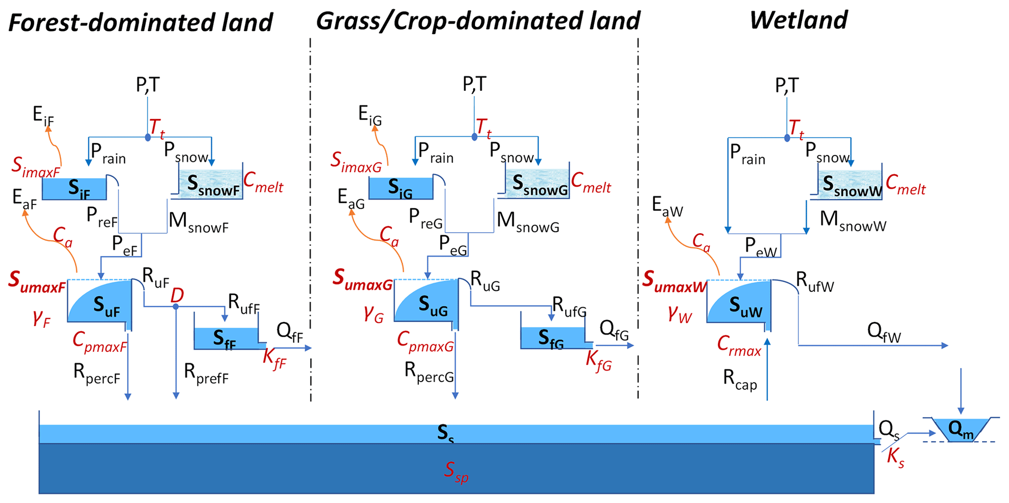
Figure 2 Model structure of the integrated model discretized into three-parallel hydrological response units (HRUs), i.e. forest, grassland and wetland in each precipitation zone (P1–P4). The light-blue boxes indicate the hydrologically active individual storage volumes. The dark-blue box indicates the hydrologically passive storage volume S_s,p. The arrow lines indicate water fluxes, and the model parameters are shown in red. All the symbols are described in Table S4 in the Supplement.

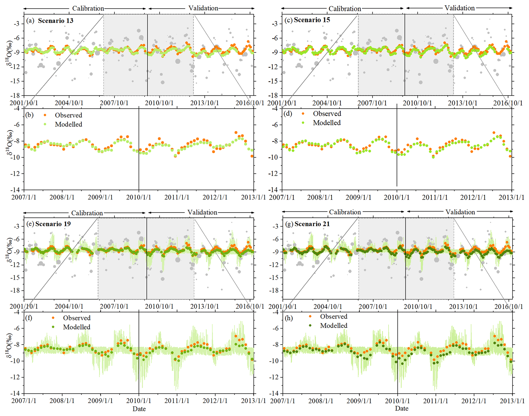
Figure 3 The time series of stream δ¹⁸O reproduced by models P-SAS (scenarios 13 and 15) and IM-SAS-D (scenarios 19 and 21) based on different calibration strategies. The IM-SAS-D model is based on simultaneous calibration to δ¹⁸O and the streamflow signatures, i.e. calibration strategies $C_{{\mathit{\delta }}^{\mathrm{18}}\mathrm{O},Q}$ (scenario 19) and $C_{{\mathit{\delta }}^{\mathrm{18}}\mathrm{O}{,}^{\mathrm{3}}\mathrm{H},Q}$ (scenario 21), for the model calibration and evaluation periods. (a) Observed δ¹⁸O signals in precipitation (light-grey dots; the sizes of the dots indicate the precipitation volume) and observed stream δ¹⁸O signals (orange dots) as well as the most balanced modelled δ¹⁸O signal in the stream (light-green dots) for scenario 13 from calibration strategy $C_{{\mathit{\delta }}^{\mathrm{18}}\mathrm{O}}$. (b) Zoom-in of observed and modelled δ¹⁸O signals in the stream for the 1 January 2007–31 December 2012 period for scenario 13. (c) Observed δ¹⁸O signals in precipitation and in the stream, same as in panel (a), and the modelled stream δ¹⁸O signals (relatively darker green dots) for scenario 15 from calibration strategy $C_{{\mathit{\delta }}^{\mathrm{18}}{\mathrm{O},}^{\mathrm{3}}\mathrm{H}}$. (d) Zoom-in of observed and modelled δ¹⁸O signals in the stream for the 1 January 2007–31 December 2012 period for scenario 15. (e) Observed δ¹⁸O signals in precipitation and in the stream, same as in panel (a), and the modelled stream δ¹⁸O signals (relatively darker green dots) for scenario 19 and the 5th and 95th percentiles of all retained Pareto optimal solutions obtained from calibration strategy $C_{{\mathit{\delta }}^{\mathrm{18}}\mathrm{O},Q}$ (light-green-shaded area). (f) Zoom-in of observed and modelled δ¹⁸O signals in the stream for the 1 January 2007–31 December 2012 period for scenario 19. (g) Observed δ¹⁸O signals in precipitation and in the stream, same as in panel (a), and the modelled stream δ¹⁸O signals (relatively darker green dots) for scenario 21 and the 5th and 95th percentiles of all retained Pareto optimal solutions obtained from calibration strategy $C_{{\mathit{\delta }}^{\mathrm{18}}\mathrm{O}{,}^{\mathrm{3}}\mathrm{H},Q}$ (light-green-shaded area). (h) Zoom-in of observed and modelled δ¹⁸O signals in the stream for the 1 January 2007–31 December 2012 period for scenario 21.

Tracer transport model

δ¹⁸O and ³H were routed through the above-described storage components of both the P-SAS and IM-SAS (Fig. 2) models by sampling the observed (i.e. Q in P-SAS) and modelled outflow volumes (i.e. E_a in P-SAS and all outflows in IM-SAS) that leave the individual components at each time step t (d) (e.g. M_snow, R_perc, E_a) from the individual water volumes of different ages T (d) that are stored in the associated storage component (e.g. S_snow, S_u) at each time step according to an SAS function. The distribution of water volumes of different ages in each storage component, i.e. the RTD, depends on the past sequence of inflows I (mm d⁻¹) and outflows O (mm d⁻¹) and therefore varies over time. As a consequence of being sampled from RTDs that evolve over time, both I and O are correspondingly characterized by water age distributions (or TTDs) that change over time. A straightforward implementation of this SAS concept is facilitated by the formulation of age-ranked storages S_T(T,t) (mm). As emphasized by Benettin et al. (2017), S_T(T,t) is described as “at any time t the cumulative volumes of water in a storage component as ranked by their age T”. Correspondingly, the total I and the total O volumes from different storages can be expressed in terms of their cumulative, age-ranked volumes I_T(T,t) and O_T(T,t) (mm d⁻¹). At any time, closing the resulting water age balance for each storage component j (e.g. S_snow, S_u) also leads to an updated age-ranked storage $S_{T,j}(T,t)$ for that component, formulated as (Benettin et al., 2015a; Botter et al., 2011; Harman, 2015; Van Der Velde et al., 2012)

$$\begin{array}{}\text{(9)}& \begin{array}{rl}& {\displaystyle \frac{\partial S_{T,j}\left(T,t\right)}{\partial t}}+{\displaystyle \frac{\partial S_{T,j}\left(T,t\right)}{\partial T}}=\\ & {\sum }_{n=\mathrm{1}}^N{I}_{T,n,j}\left(T,t\right)-{\sum }_{m=\mathrm{1}}^M{O}_{T,m,j}\left(T,t\right),\end{array}\end{array}$$

where $\partial S_T/\partial T$ is the ageing process of water in storage. Here, the water age balance (Eq. 7) was formulated individually for each storage reservoir j, also accounting for different numbers N of storage component inflows I (e.g. P_rain, M_snow, R_perc) and numbers M of outflows O (e.g. R_perc, R_pref, E_a) (Fig. 2), similar to previous studies (e.g. Hrachowitz et al., 2021). For a daily modelling time step, in the water age balance it can be assumed that precipitation P(t) that falls on day t is characterized by an age T=0. This implies for the age-ranked inflow that $I_{T,P,j}(\mathrm{0},t)=P_T(\mathrm{0},t)=P\left(t\right)$. Note that all other age-ranked inflows $I_{T,n,j}(T,t)$ that enter a storage component are equivalent to the corresponding age-ranked outflows $O_{T,m,j}(T,t)$ that leave a “higher” storage component.

Depending on the total volume of outflow O_m,j(t) and the cumulative distribution of ages $P_{\mathrm{o},m,j}(T,t)$ of that flow, an age-ranked outflow $O_{T,m,j}(T,t)$ for each flux m released from each storage component j can be defined as

$$\begin{array}{}\text{(10)}& O_{T,m,j}\left(T,t\right)=O_{m,j}\left(t\right)P_{\mathrm{o},m,j}\left(T,t\right).\end{array}$$

While the outflow O_m,j(t) from any storage component j is computed for each time step t by the hydrological model described above, the associated $P_{\mathrm{o},m,j}(T,t)$ cannot be assumed to be known as it is controlled by the temporally evolving distribution of water ages present in that storage component $S_{T,j}(T,t)$ at t. However, the temporally variable $P_{\mathrm{o},m,j}(T,t)$ can be inferred for each time step t by defining, for each storage j and for each outflow m released from j, an SAS function ${\mathit{\omega }}_{\mathrm{o},m,j}$ together with its cumulative form ${\mathrm{\Omega }}_{\mathrm{o},m,j}$. These functions then describe how the water volumes of different ages, stored in component j at time t, i.e. $S_{T,j}(T,t)$, are sampled and combined into the corresponding total outflow volume O_m,j(t):

$$\begin{array}{}\text{(11)}& P_{\mathrm{o},m,j}\left(T,t\right)={\mathrm{\Omega }}_{\mathrm{o},m,j}\left(S_{T,j}\left(T,t\right),t\right).\end{array}$$

The probability density function $p_{\mathrm{o},m,j}(T,t)$ associated with the cumulative distribution of ages $P_{\mathrm{o},m,j}(T,t)$ then represents the TTD of that outflow and can be written as

$$\begin{array}{}\text{(12)}& p_{\mathrm{o},m,j}\left(T,t\right)={\mathit{\varpi }}_{\mathrm{o},m,j}\left(S_{T,j}\left(T,t\right),t\right){\displaystyle \frac{\partial S_{T,j}}{\partial T}}.\end{array}$$

Conservation of mass dictates that

$$\begin{array}{}\text{(13)}& {\mathrm{\Omega }}_{\mathrm{o},m,j}\left(S_{T,j}\left(T,t\right)\to S_j\left(t\right),t\right)=\mathrm{1},\end{array}$$

where S_j (mm) is the total volume of water stored in component j at time t. The resulting need to rescale ${\mathit{\omega }}_{\mathrm{o},m,j}$ for each time step was avoided here by instead normalizing and therefore bounding the age-ranked storage to the interval [0, 1] according to

$$\begin{array}{}\text{(14)}& S_{T,\mathrm{norm},j}\left(T,t\right)={\displaystyle \frac{S_{T,j}\left(T,t\right)}{S_j\left(t\right)}}.\end{array}$$

Note that $S_{T,\mathrm{norm},j}$ also represents the RTD of storage component j at time t.

For the P-SAS model implementation in this study, we used power law distributions with one parameter to sample streamflow (k_Q) and evaporation (k_E), respectively, as described by Benettin et al. (2017). In contrast, we used uniform distributions in the form of ω= const. as an SAS function in each storage component in the IM-SAS model implementations, as previously shown to be effective in many studies (e.g. Birkel et al., 2011; van der Velde et al., 2015; Benettin et al., 2015b, 2017; Ala-Aho et al., 2017; Kuppel et al., 2018; Rodriguez et al., 2018). The latter implies random sampling together with the assumption that each storage component is fully mixed and that there is no preference for sampling younger or older water. However, note that, due to distinct storage capacities and timescales of the individual storage components, the “combined” SAS functions of all storage components will not lead to an overall fully mixed system response. Uniform SAS functions were chosen here over other shapes, such as beta distributions (e.g. van der Velde et al., 2012; Hrachowitz et al., 2021), as they do not need additional model parameters and avoid the need for explicit calculation of TTDs at each model time step to route tracers through the model (Benettin et al., 2015b), thereby drastically reducing computer memory requirements and computational time (Benettin et al., 2022).

To adequately damp tracer input signals, suitable system storage volumes have to be defined as calibration parameters. In the P-SAS implementation, the parameter S_tot is used, reflecting the initial total system storage (e.g. Benettin et al., 2017). In contrast, the IM-SAS implementations made use of additional and hydrologically passive storage volumes (e.g. Christophersen and Wright, 1981; Birkel et al., 2010; Hrachowitz et al., 2015, 2016) that physically represent groundwater volumes below the river bed, as illustrated by Zuber (1986; Fig. 1 therein). Such a passive water storage volume S_s (mm), characterized by d$S_{\mathrm{s},\mathrm{p}}/\mathrm{d}t=\mathrm{0}$, was thus added as a calibration parameter to the active groundwater storage S_s (Fig. 2). While the outflow Q_s from the groundwater storage is exclusively regulated by the temporally varying storage volume in S_s (Eq. S9 in the Supplement), the tracer and age composition of that outflow is also randomly sampled from the total groundwater storage volume $S_{\mathrm{s},\mathrm{tot}}=S_{\mathrm{s}}+S_{\mathrm{s},\mathrm{p}}$.

The δ¹⁸O and ³H concentrations were then routed through each individual storage component according to (e.g. Harman, 2015; Benettin et al., 2017)

$$\begin{array}{}\text{(15)}& \begin{array}{rl}& C_{\mathrm{o},m,j}\left(t\right)={\int }_{\mathrm{0}}^{S_j}{C}_{\mathrm{s},j}\left(S_{T,j}\right(T,t),t){\mathit{\omega }}_{\mathrm{o},m,j}\\ & \left(S_{T,j}\left(T,t\right),t\right)e^{-\mathit{\lambda }T}\mathrm{d}{S}_T,\end{array}\end{array}$$

where $C_{\mathrm{o},m,j}$ is the tracer concentration in outflow m from storage component j at time t; C_s,j is the tracer concentration of water in storage at time t; and λ is the radioactive decay constant (λ=0 d⁻¹ for δ¹⁸O and λ=0.00015 d⁻¹ for ³H).

4.2 Model implementation

4.2.1 Spatially lumped model implementation

The original argument that the use of seasonally variable tracers underestimates water ages was exclusively based on lumped, time-invariant implementations of sine-wave and convolution integral models (Stewart et al., 2010). For a baseline comparison and to check whether the above conclusion would also have been reached for our study basin using the same methods, here we similarly implemented the sine-wave (SW-EM, SW-GM) and convolution integral (CO-EM, CO-GM, CO-2EM, CO-3EM, CO-EPM) models in a spatially lumped way. For this baseline case the catchment average tracer input was estimated as the spatially weighted mean from the four precipitation zones P1–P4 as described in Sect. 3.2. The calibration parameters of the CO implementations are shown in Table 2.

The P-SAS model (Table 3) and the spatially lumped implementation of the integrated model (IM-SAS-L) were also forced with the same spatially averaged input. In addition, the spatial fractions for IM-SAS-L of the grassland and wetland HRUs, respectively, were set to 0, and the entire study basin was therefore represented by one HRU, which is equivalent to the forest HRU described in the distributed model, similar to many traditional lumped formulations of process-based conceptual models (Bouaziz et al., 2021; Clark et al., 2008; Fenicia et al., 2006; Fovet et al., 2015; Seibert et al., 2010). This implementation has 11 calibration parameters (Table 3).

4.2.2 Spatially distributed model implementation

To balance the need for spatial detail to some extent with the adverse effects of increased parameter uncertainty (e.g. Beven, 2006) and computational capacity (in particular for the calculation of TTDs), here we implemented the integrated model in parallel (IM-SAS-D) in the four precipitation zones P1–P4 and forced it with the corresponding input (e.g. P, δ¹⁸O and ³H) for each precipitation zone as described in Sect. 3.2. Each precipitation zone was further discretized (1) into 100 m elevation zones for a stratified representation of the snow storage S_snow (e.g. Mostbauer et al., 2018) and (2) into three HRUs, i.e. forest, grassland and wetland (Fig. 2; e.g. Gharari et al., 2014; Hanus et al., 2021). Rainwater P_rain and meltwater M_snow from the different elevation zones were aggregated according to their associated spatial weights in each elevation zone. This total liquid water input was then routed through the three parallel HRUs. The classification into the three HRUs was based on HAND (Gharari et al., 2011) and land cover. While landscape elements with HAND <5 m were classified as wetland, all other parts of the landscape were classified as forest or grassland according to land use data. In total, there are therefore 12 individual, parallel model components, i.e. three HRUs in each of the four precipitation zones, not counting the elevation zones for the snow module. All flux and storage variables of the 12 components are weighted according to their areal fractions. While each of the three HRUs was characterized by individual parameters (e.g. Gao et al., 2016; Prenner et al., 2018), the same parameter values were used in all four precipitation zones in a distributed moisture-accounting approach (e.g. Ajami et al., 2004; Euser et al., 2015; Hulsman et al., 2021b; Roodari et al., 2021). Overall, the spatially distributed implementation has 19 model parameters, including 5 global parameters (T_t, C_melt, C_a, K_s and S_s,p) that are identical for each HRU and 14 HRU-specific parameters (Table 3; Fig. 2).

4.3 Model calibration and post-calibration evaluation

The models were run at a daily time step where the observed volume-weighted monthly tracer concentration in precipitation was used as model input for each day of that month together with the daily data of precipitation. Model performance was evaluated based on the MSE as an error metric. The time-invariant, lumped convolution integral models, using uniform prior parameter distributions as shown in Table 2, were individually calibrated to the observed δ¹⁸O (calibration strategy $C_{{\mathit{\delta }}^{\mathrm{18}}\mathrm{O}}$; Table 2) and ³H stream water concentrations ($C_{{}^{\mathrm{3}}\mathrm{H}}$), respectively. In contrast, a multi-objective calibration approach was applied for the integrated IM-SAS models to simultaneously reproduce streamflow volumes and tracer concentrations thereof (e.g. ³H and/or δ¹⁸O). Briefly, the model parameters were calibrated by using the Borg MOEA (Borg multiobjective evolutionary algorithm) (Hadka and Reed, 2013) and were based on uniform prior distributions (Table 3). The model performances were evaluated based on the models' ability to simultaneously reproduce multiple signatures of streamflow and signatures of tracer dynamics as shown in Table 3. The sets of Pareto optimal solutions obtained from the calibration procedures were then retained as acceptable solutions for the subsequent analysis. To compare the water age distributions (i.e. TTDs and RTDs) and thus to test the research hypothesis, different calibration strategies – $C_{{\mathit{\delta }}^{\mathrm{18}}\mathrm{O},Q}$, $C_{{}^{\mathrm{3}}\mathrm{H},Q}$ and $C_{{\mathit{\delta }}^{\mathrm{18}}\mathrm{O}{,}^{\mathrm{3}}\mathrm{H},Q}$ – were adopted (Table 3). While in strategy $C_{{\mathit{\delta }}^{\mathrm{18}}\mathrm{O},Q}$ the models were calibrated to simultaneously reproduce signatures of streamflow and δ¹⁸O, $C_{{}^{\mathrm{3}}\mathrm{H},Q}$ combined the streamflow signatures with ³H. In strategy $C_{{\mathit{\delta }}^{\mathrm{18}}\mathrm{O}{,}^{\mathrm{3}}\mathrm{H},Q}$ the model was finally calibrated to simultaneously reproduce the six streamflow signatures as well as δ¹⁸O and ³H dynamics. For each strategy, all the performance metrics were also combined into an overall performance metric based on the Euclidian distance D_E, where D_E=0 indicates a perfect fit. To find a somewhat balanced solution in the absence of more detailed information, all the individual performance metrics were equally weighted here (e.g. Hrachowitz et al., 2021; Hulsman et al., 2021b):

$$\begin{array}{}\text{(16)}& D_{\mathrm{E}}=\sqrt{{\displaystyle \frac{\mathrm{1}}{\mathrm{2}}}\left({\displaystyle \frac{{\sum }_{n=\mathrm{1}}^N{\left(E_{\mathrm{MSE},Q,n}\right)}^{\mathrm{2}}}{N}}+{\displaystyle \frac{{\sum }_{m=\mathrm{1}}^M{\left(E_{\mathrm{MSE},\mathrm{tracer},m}\right)}^{\mathrm{2}}}{M}}\right)},\end{array}$$

where N=6 is the number of performance metrics with respect to streamflow ($E_{\mathrm{MSE},Q,n}$) and M is the number of performance metrics for tracers ($E_{\mathrm{MSE},\mathrm{tracer},m}$) in each combination (e.g. M=1 for $C_{{\mathit{\delta }}^{\mathrm{18}}\mathrm{O},Q}$ and $C_{{}^{\mathrm{3}}\mathrm{H},Q}$; M=2 for $C_{{\mathit{\delta }}^{\mathrm{18}}\mathrm{O}{,}^{\mathrm{3}}\mathrm{H},Q}$). Note that the different units and thus different magnitudes of residuals introduce some subjectivity in finding the most balanced overall solution according to D_E (Eq. 16). However, a preliminary sensitivity analysis with varying weights for the individual performance metrics in D_E suggested limited influence on the overall results and is thus not further reported here.

After a warm-up period (1 January 1978–30 September 2001), the models were calibrated for the 1 October 2001–31 December 2009 period. The calibration period was chosen so that observations of all three calibration variables, i.e. Q, ³H and δ¹⁸O, are available for the entire calibration period to allow a consistent comparison. The long model warm-up period was deemed necessary to meaningfully approximate the model initial conditions due to the potential and a priori unknown relevance of old water in the study basin and thus to avoid underestimation of water ages inferred from ³H data. The Pareto optimal solutions (parameter sets) of the Neckar basin model were then used to test the model in the post-calibration evaluation period 1 January 2010–31 December 2016. In addition, the model was tested for its ability to represent spatial differences in the hydrological response by evaluating it against streamflow observations in three sub-catchments (C1–C3) of the Neckar without further re-calibration, where each one of them largely represents the hydrological response from one of the precipitation zones (Fig. 1). The water age distributions, i.e. TTDs and RTDs, extracted from the individual models and calibration strategies were then estimated based on the corresponding sets of Pareto optimal solutions obtained for each calibration strategy.

5 Results

5.1 Model performance

The stream tracer responses of the lumped baseline models were found to be broadly consistent with the available observations (Table 4). For the SW models (scenarios 1 and 2), in particular, the sine wave fitted to the stream water δ¹⁸O observations provides a robust characterization of the observed signal with MSE${}_{{\mathit{\delta }}^{\mathrm{18}}\mathrm{O}}=\mathrm{0.121}$ ‰ and 0.144 ‰ for the calibration and model evaluation periods, respectively (Fig. S5 in the Supplement). Similarly, the CO models (scenarios 3, 5, 7, 9 and 11) reproduced the overall pattern of seasonal fluctuations and the degree of dampening of the δ¹⁸O response (Supplement Fig. S6). The best-performing model, the CO-3EM model, was characterized by MSE${}_{{\mathit{\delta }}^{\mathrm{18}}\mathrm{O}}=\mathrm{0.171}$ ‰ and 0.191 ‰ for the calibration and model evaluation periods, respectively, while, in comparison, the CO-EM implementation exhibited considerably higher errors with MSE${}_{{\mathit{\delta }}^{\mathrm{18}}\mathrm{O}}=\mathrm{0.327}$ ‰ and 0.432 ‰ (Table 4). When used with ³H data (scenarios 4, 6, 8, 10 and 12), the CO models do capture the general decrease in the magnitude of stream water ³H concentrations, although fluctuations at shorter timescales are not well reproduced (Fig. S7 in the Supplement). The CO-2EM model gives the best performance with MSE${}_{{}^{\mathrm{3}}\mathrm{H}}=\mathrm{5.171}$ and 3.964 TU² for the calibration and evaluation periods, respectively, while the CO-EPM model resulted in MSE${}_{{}^{\mathrm{3}}\mathrm{H}}=\mathrm{5.926}$ and 5.115 TU² (Table 4). It is also noted that the models already mimic the ³H response well in the 1978–2001 pre-calibration model warm-up period.

Table 4 Performance metrics of the 12 time-invariant, lumped SW and CO model implementations for the 2001–2009 calibration period (cal.) and the 2010–2016 model evaluation period (val.). For brevity, only the values for the most balanced solution are shown here. ^* The MSE values provided for C_x describe the sine-wave fits of both the precipitation and streamflow δ¹⁸O signals, respectively.

The P-SAS implementations (scenarios 13–15; Table 5; Figs. 3a–d and 4a–d) show a somewhat higher skill in reproducing the dampening of the δ¹⁸O response with MSE${}_{{\mathit{\delta }}^{\mathrm{18}}\mathrm{O}}=$ 0.069 ‰–0.078 ‰ for the calibration period and 0.215 ‰–0.231 ‰ for the evaluation period, respectively, together with a general decrease in the magnitude of stream water ³H with MSE${}_{{}^{\mathrm{3}}\mathrm{H}}\mathit{<}\mathrm{3}$ TU². In contrast to the above, the implementations of the integrated model IM-SAS (Table 5) aim not only to reproduce the δ¹⁸O or ³H stream signals, but to additionally and simultaneously describe the hydrological response (Table 5). Both the lumped IM-SAS-L (scenario 16; Fig. S8a, b in the Supplement) and the distributed IM-SAS-D (scenario 19; Fig. 3e, f) reproduce the seasonal fluctuations as well as the degree of dampening of the δ¹⁸O signals with MSE${}_{{\mathit{\delta }}^{\mathrm{18}}\mathrm{O}}=$ 0.079 ‰–0.083 ‰ for the calibration period and 0.273 ‰–0.332 ‰ for the evaluation period, similar to or better than the baseline SW or CO models. The IM-SAS models also describe the evolution of the ³H stream signals rather well (scenarios 17 and 20). With MSE${}_{{}^{\mathrm{3}}\mathrm{H}}\mathit{<}\mathrm{3}$ TU², IM-SAS-L (Fig. S9 in the Supplement) and IM-SAS-D (Fig. 4e–h) not only outperform the baseline models with respect to the overall magnitude of ³H, but, in spite of somewhat underestimating the magnitudes of seasonal amplitudes, also provide a better representation of these intra-annual fluctuations. Similarly to the SW and CO baseline models, both the P-SAS and IM-SAS implementations also capture the overall decline of the stream water ³H levels in the 1978–2001 pre-calibration model warm-up period very well. The simultaneous calibration to the hydrological response and the δ¹⁸O and ³H stream signals (scenarios 18 and 21) led to a comparable model skill to reproduce the tracer signals. In addition to the tracer concentrations, all IM-SAS implementations also reproduce the main features of the hydrological response (Table 5). More specifically, the modelled hydrographs in particular describe well the timing of peaks and the shape of recessions, although in some cases peak flows were underestimated and low flows overestimated, as shown for scenario 21 in Fig. 5 (for scenarios 16–20, see Figs. S10–S14 in the Supplement). The resulting MSE_Q remains ≤0.336 mm² d⁻² across all IM-SAS implementations (scenarios 16–21). Crucially, the models also reproduce well the other observed streamflow signatures, such as the flow duration curves (MSE_FDCQ≤0.047 mm² d⁻²; Fig. 5d), the seasonal runoff coefficients (MSE_RC≤ 0.008; Fig. 5e) and the autocorrelation functions (MSE_ACQ≤0.007; Fig. 5f). The model, calibrated on the overall response of the Neckar basin, also exhibited considerable skill in representing spatial differences in the hydrological response by reproducing observed streamflow in the three sub-catchments (C1–C3) similarly well (Fig. 6) without any further re-calibration.

Table 5 Performance metrics of the nine P-SAS and IM-SAS model scenarios for the 2001–2009 calibration period (cal.) and the 2010–2016 model evaluation period (val.). For brevity, only the values for the most balanced solution, i.e. the lowest D_E (Eq. 16), are shown here. The ranges of all the performance metrics for the full set of Pareto optimal solutions for the multi-objective calibration cases (scenarios 15–21) are provided in Table S5 in Supplement.

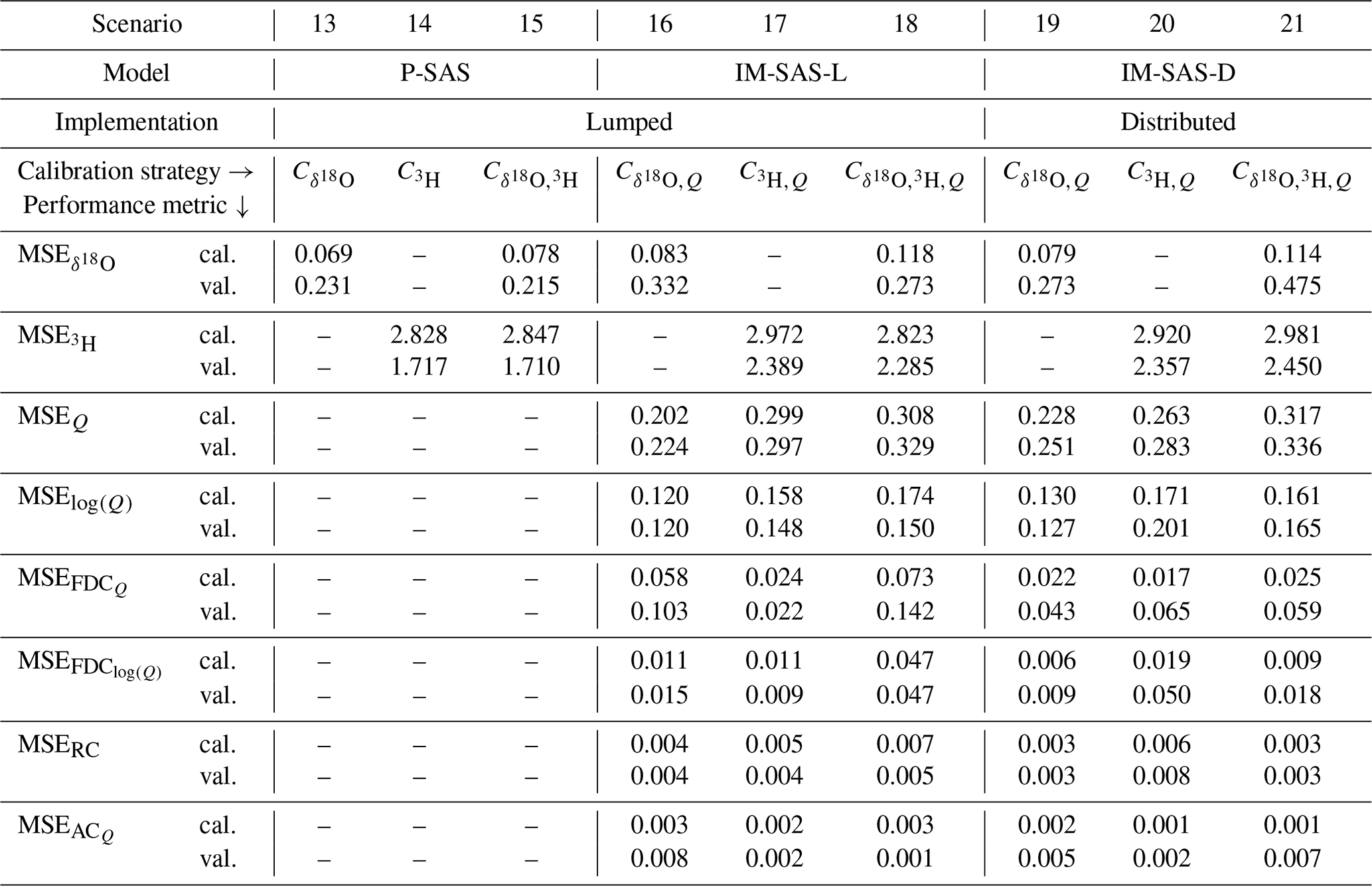
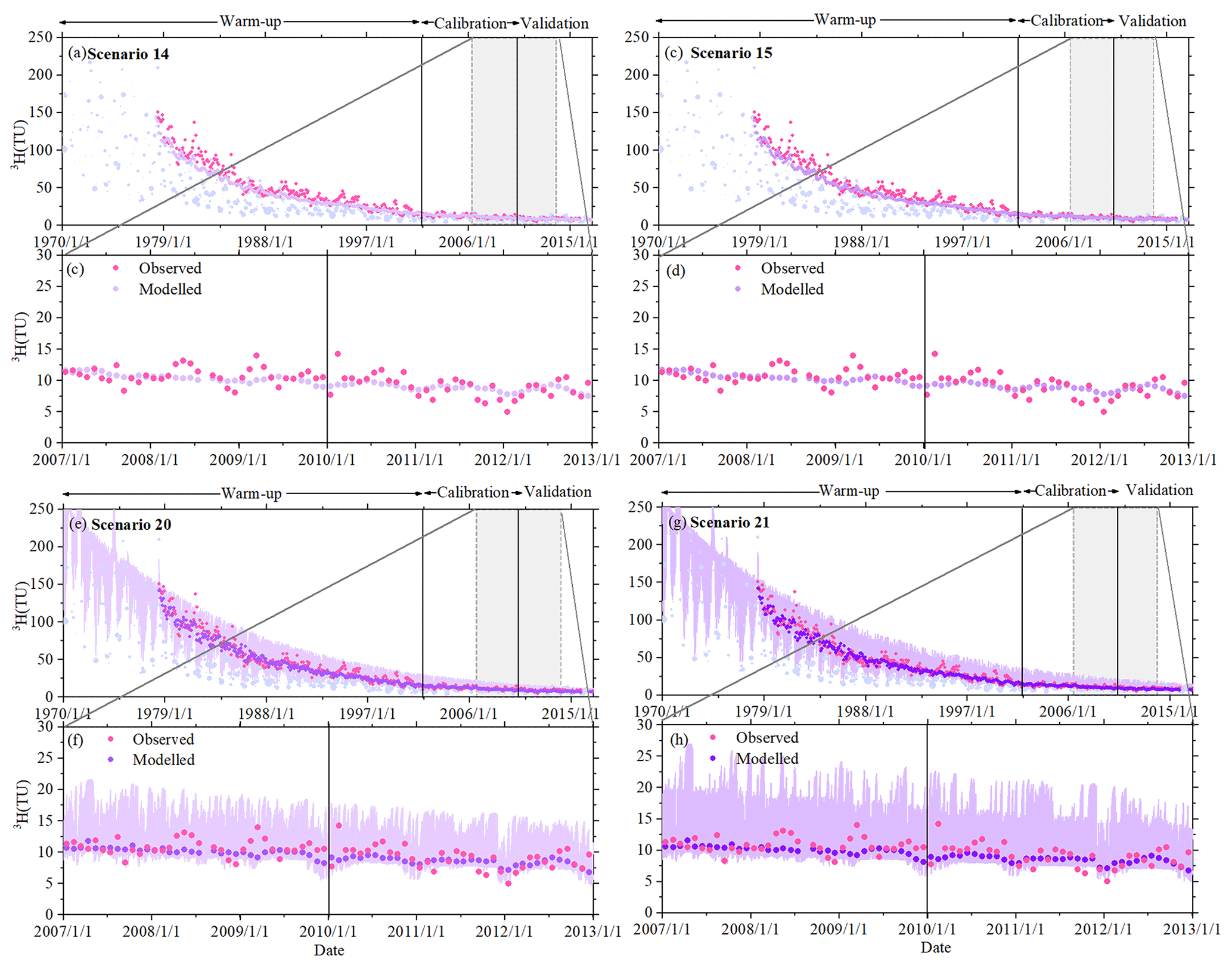
Figure 4 The time series of stream ³H reproduced by models P-SAS (scenarios 14 and 15) and IM-SAS-D (scenarios 20 and 21) based on different calibration strategies. The IM-SAS-D model is based on simultaneous calibration to ³H and the streamflow signatures, i.e. calibration strategies $C_{{}^{\mathrm{3}}\mathrm{H},Q}$ (scenario 20) and $C_{{\mathit{\delta }}^{\mathrm{18}}\mathrm{O}{,}^{\mathrm{3}}\mathrm{H},Q}$ (scenario 21) for the model calibration and evaluation periods. (a) Observed ³H signals in precipitation (light-blue-purple dots; the sizes of the dots indicate the precipitation volume) and observed stream ³H signals (pink dots) as well as the most balanced modelled ³H signal in the stream (light-purple dots) for scenario 14 from calibration strategy $C_{{}^{\mathrm{3}}\mathrm{H}}$. (b) Zoom-in of observed and modelled ³H signals in the stream for the 1 January 2007–31 December 2012 period for scenario 14. (c) Observed ³H signals in precipitation and in the stream, same as in panel (a), and the modelled stream ³H signals (relatively darker purple dots) for scenario 15 from calibration strategy $C_{{\mathit{\delta }}^{\mathrm{18}}{\mathrm{O},}^{\mathrm{3}}\mathrm{H}}$. (d) Zoom-in of observed and modelled ³H signals in the stream for the 1 January 2007–31 December 2012 period for scenario 15. (e) Observed ³H signals in precipitation and in the stream, same as in panel (a), and the modelled stream ³H signals (relatively darker purple dots) for scenario 20 and the 5th and 95th percentiles of all retained Pareto optimal solutions obtained from calibration strategy $C_{{}^{\mathrm{3}}\mathrm{H},Q}$ (light-purple-shaded area). (f) Zoom-in of observed and modelled ³H signals in the stream for the 1 January 2007–31 December 2012 period for scenario 20. (g) Observed ³H signals in precipitation and in the stream, same as in panel (a), and the modelled stream ³H signals (relatively darker green dots) for scenario 21 and the 5th and 95th percentiles of all retained Pareto optimal solutions obtained from calibration strategy $C_{{\mathit{\delta }}^{\mathrm{18}}\mathrm{O}{,}^{\mathrm{3}}\mathrm{H},Q}$ (light-green-shaded area). (h) Zoom-in of observed and modelled ³H signals in the stream for the 1 January 2007–31 December 2012 period for scenario 21.

5.2 Model parameters

Parameters of the SW or CO baseline models (scenarios 1–12) directly define the shapes of parametric TTDs and thus the associated metrics of water age, such as MTTs following Eqs. (3)–(7). The CO models representing ³H signals (scenarios 4, 6, 8, 10 and 12) are characterized by values of parameters β₁, β₂ and β₃ that are a factor of up to ∼10 higher than the same parameters of models calibrated to δ¹⁸O signals (Table 2). For example, β₁=513 d for the CO-EM in scenario 3 and 3795 d in scenario 4.

The individual parameters of the P-SAS and IM-SAS model implementations (scenarios 13–21), in contrast, do not directly define parametric TTDs, nor can they readily and directly be linked to water ages. However, it has been shown previously that the sizes of water storage volumes are an important control on water ages (e.g. Harman, 2015) and that, in particular, total storage volumes, represented by parameter S_tot in P-SAS, and the hydrologically passive storage volumes, represented by parameter S_s,p in the IM-SAS models, are key to regulating older water ages in many systems (e.g. Hrachowitz et al., 2016). Calibration of P-SAS to δ¹⁸O in scenario 13 suggested S_tot∼15 595 mm, while calibration of the lumped IM-SAS-L to δ¹⁸O and streamflow ($C_{{\mathit{\delta }}^{\mathrm{18}}\mathrm{O},Q}$) in scenario 16 led to a moderately well-identifiable range of this parameter ($S_{\mathrm{s},\mathrm{p}}\sim$ 4107–10 029 mm) across all Pareto optimal solutions and the same order of magnitude as P-SAS (Fig. 7a; Table 3). Reflecting the water storage capacity in the unsaturated root zone, which is an important control on younger water ages (Hrachowitz et al., 2021), the parameter S_umaxF was found to range between ∼ 314 and 415 mm (Fig. 7b; Table 3) for the same IM-SAS-L scenario. The calibration of the same models to ³H (scenarios 14 and 17) resulted in similar parameter ranges of S_tot∼16 638 mm, $S_{\mathrm{s},\mathrm{p}}\sim$ 3924–9339 mm (Fig. 7a) and, albeit slightly lower, S_umaxF∼ 236–355 mm (Fig. 7b). The similarities between these two scenarios are also reflected in the parameter ranges obtained from the simultaneous calibration to δ¹⁸O and ³H (C${}_{{\mathit{\delta }}^{\mathrm{18}}{\mathrm{O},}^{\mathrm{3}}\mathrm{H},Q}$) in scenarios 15 and 18. The calibration of the distributed IM-SAS-D model following all three calibration strategies in scenarios 19–21 resulted in values for $S_{\mathrm{s},\mathrm{p}}\sim$ 3270–9011 mm (Fig. 7c) that are broadly in similar ranges to IM-SAS-L ($S_{\mathrm{s},\mathrm{p}}\sim$ 3924–13 676 mm). In contrast, the distinction into the individual HRUs led to clear differences between S_umaxF, S_umaxG and S_umaxW (Fig. 7d–f) that are reflective of the different hydrological functioning of these HRUs. Nevertheless, the area-weighted average of these parameters comes close to the equivalent parameter from the lumped model implementation (S_umaxF). The general consistency of these parameters obtained from the different calibration strategies is exacerbated by the limited differences in the most balanced solutions (smallest D_E) between the different scenarios. For example, the most balanced solutions of S_s,p fall between ∼ 4000 and 5000 mm for all IM-SAS scenarios (16–21) (Fig. 7a, c). All the other parameters, which are less clearly related to water ages, exhibit different levels of variation across the individual scenarios but do not follow any clear and systematic pattern (Table 3).

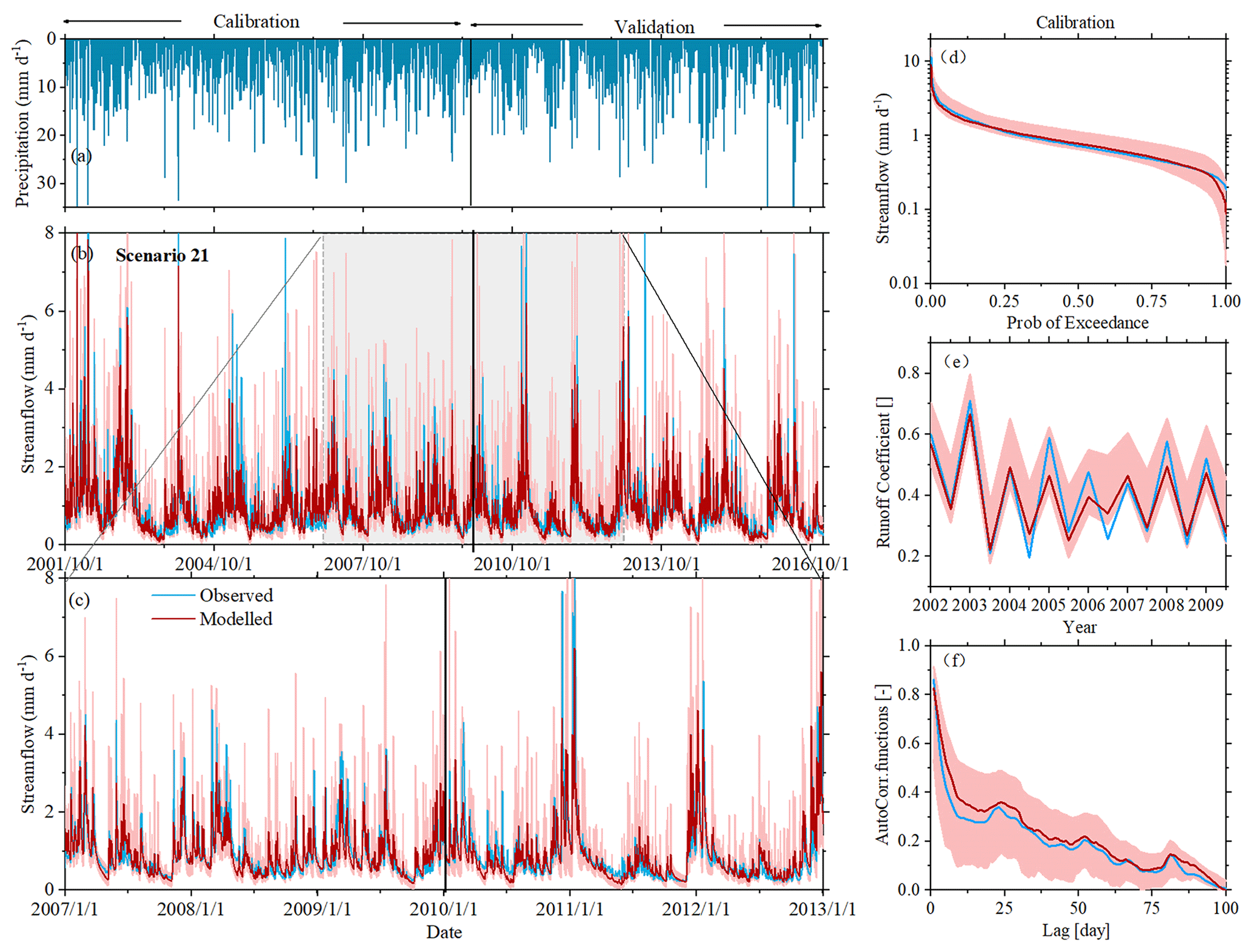
Figure 5 Hydrograph and selected hydrological signatures reproduced by IM-SAS-D following a simultaneous calibration to the hydrological response, δ¹⁸O and ³H (C${}_{{\mathit{\delta }}^{\mathrm{18}}{\mathrm{O},}^{\mathrm{3}}\mathrm{H},Q}$; scenario 21). (a) Time series of observed daily precipitation: observed and modelled (b) daily streamflow (Q), where the red line indicates the most balanced solution, i.e. the lowest D_E, and the red-shaded area indicates the 5th or 95th inter-quantile range obtained from all Pareto optimal solutions. (c) Streamflow zoomed in to the 1 January 2007–31 December 2012 period. (d) Flow duration curves (FDC_Q). (e) Seasonal runoff coefficients (RC_Q) and (f) autocorrelation functions of streamflow (AC_Q) for the calibration period. Blue lines indicate values based on observed streamflow (Q_o); red lines are values based on modelled streamflow (Q_m) representing the most balanced solutions. That is, the lowest D_E and the red-shaded areas show the 5th and 95th inter-quantile ranges obtained from all Pareto optimal solutions.

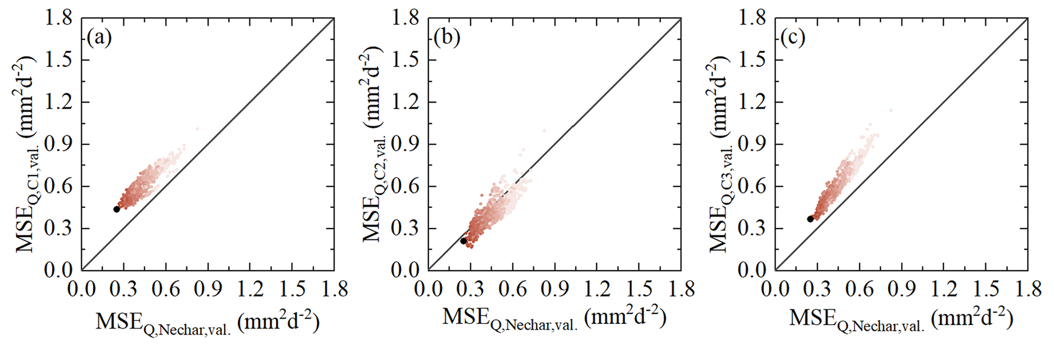
Figure 6 Selected model performances in the 1 January 2010–31 December 2016 validation period of the overall Neckar basins against the model performance in uncalibrated sub-catchments (a) Kirchentellinsfurt (C1), (b) Calw (C2) and (c) Untergriesheim (C3) based on scenario 19. The dots indicate all Pareto optimal solutions in the multi-objective model performance space. The shades from dark to light indicate the overall model performance based on the Euclidean distance D_E, with the black solutions representing the overall better solutions (i.e. smaller D_E).

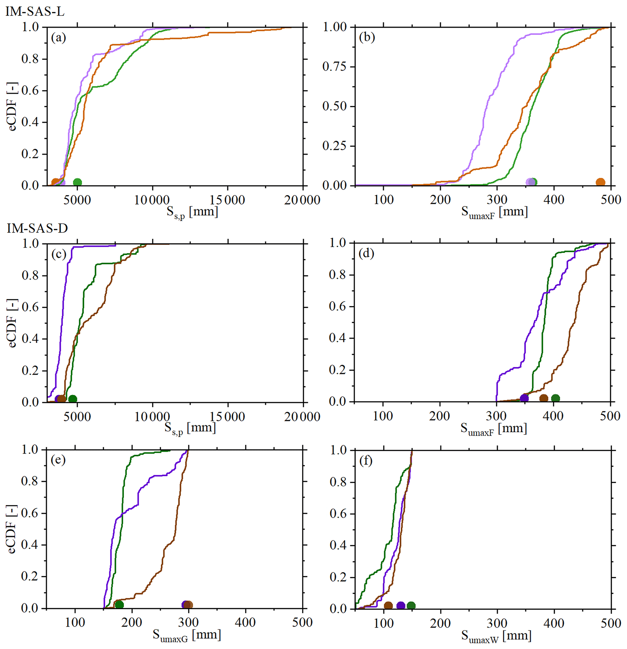
Figure 7 Pareto optimal distributions of selected parameters of the IM-SAS models (i.e. IM-SAS-L, IM-SAS-D) shown as the associated empirical cumulative distribution functions (lines). Light-green shades indicate scenario 16, light-purple shades indicate scenario 17, and light-brown shades indicate scenario 18 in panels (a) and (b). Relatively darker green shades indicate scenario 19, relatively darker purple shades indicate scenario 20, and relatively darker brown shades indicate scenario 21 in panels (c)–(f). The dots indicate the parameter values associated with the most balanced solution, i.e. the lowest D_E.

5.3 Water age distributions

Based on a δ¹⁸O amplitude ratio $A_{\mathrm{s}}/A_{\mathrm{p}}=\mathrm{0.21}$ (Table 2), the results of the SW models (scenarios 1 and 2) suggest a system that is characterized by rather young stream water with MTTs of ∼ 0.7–1.8 years, depending on the choice of TTD (Table 6; Fig. 8). The TTDs obtained from the CO models calibrated to δ¹⁸O (scenarios 3, 5, 7, 9 and 11) are broadly consistent with this, suggesting MTTs of ∼ 1.4–2.4 years. These TTDs suggest mean water ages that are up to ∼9 years lower than estimates from CO models calibrated to ³H (scenarios 4, 6, 8, 10 and 12) with MTTs of ∼ 9.4–10.4 years (Table 6; Fig. 8). For higher percentiles, the differences in water ages can even reach more than 20 years (Table 6). Correspondingly, the fractions of water younger than 3 months, F(T<3 m), exhibit considerable differences of −2 %–22% points between δ¹⁸O- and ³H-inferred estimates, which further increase to differences of 30 %–64 % for F(T<3 years).

Table 6 Metrics of streamflow TTDs derived from the 12 SW and CO model scenarios with the different associated calibration strategies, where $C_{{\mathit{\delta }}^{\mathrm{18}}\mathrm{O}}$ indicates calibration to δ¹⁸O and $C_{{}^{\mathrm{3}}\mathrm{H}}$ calibration to ³H. The TTD metrics represent the best fits of the respective time-invariant TTDs. The water fractions are shown as the fractions below a specific age T, i.e. F(T< age). The columns with the absolute difference Δ summarize the differences in TTDs from the same models calibrated to δ¹⁸O and ³H, respectively. The subscripts indicate the scenarios that are compared (e.g. Δ_3,4 compares scenarios 3 and 4). ^* Note that the fraction of water younger than 3 months F(T<3 m) is comparable to the fraction of young water as suggested by Kirchner (2016).

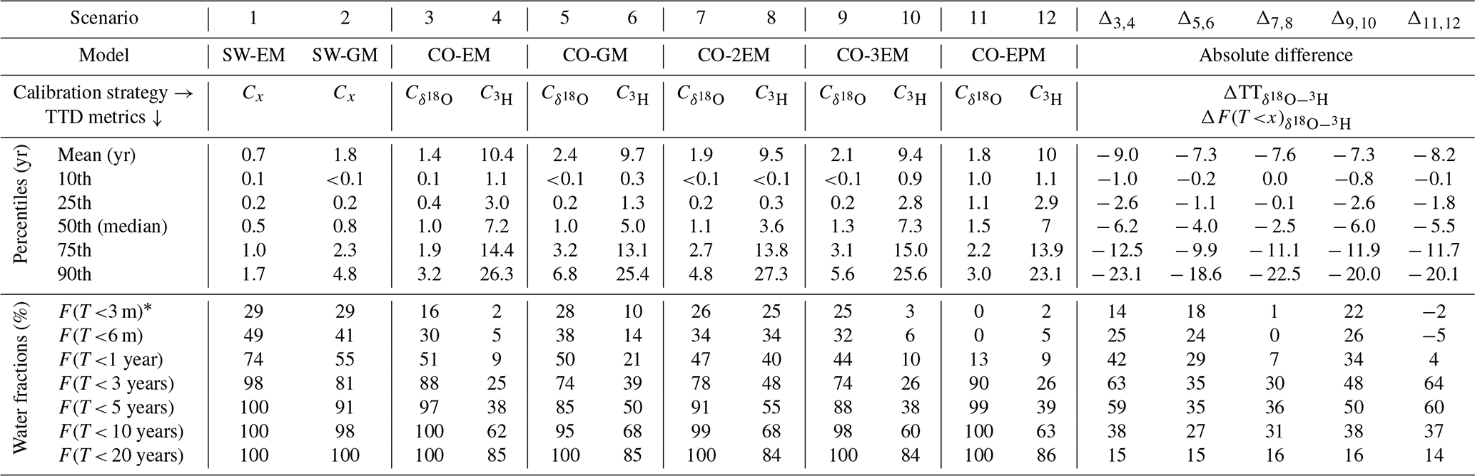
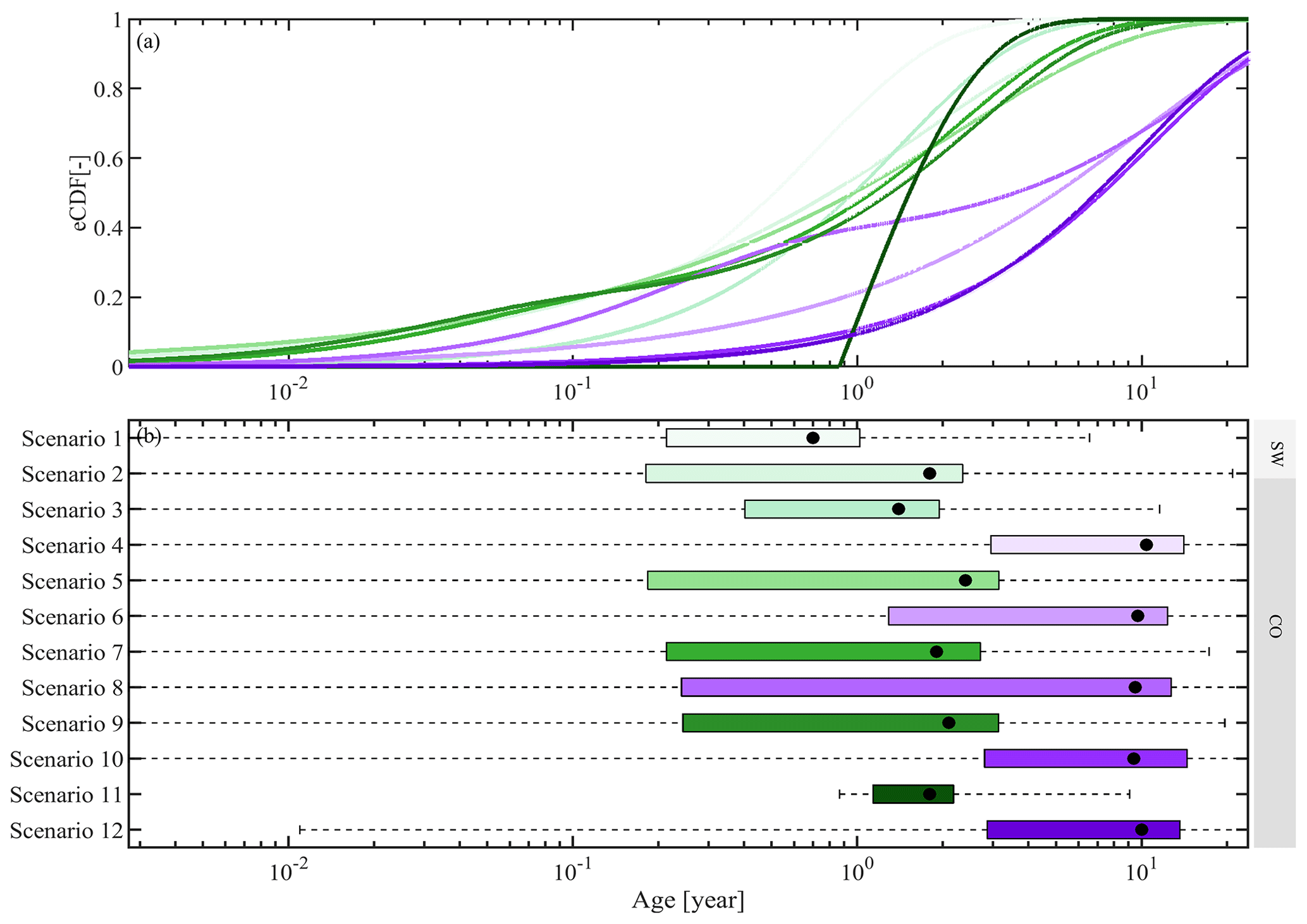
Figure 8 Streamflow TTDs derived from the 12 SW and CO model scenarios with the different associated calibration strategies based on different lumped, time-invariant models. The TTDs represent the best fits of the respective time-invariant TTDs. The green shades represent the TTDs inferred from δ¹⁸O (from lighter to darker for scenarios 1, 2, 3, 5, 7, 9 and 11) in panels (a) and (b). The purple shades represent TTDs inferred from ³H (from lighter to darker for scenarios 4, 6, 8, 10 and 12). The black dots in panel (b) indicate the mean transit time for each model scenario.

In contrast, from the implementations of the P-SAS and IM-SAS models in scenarios 13–21, it can be clearly seen that the stream water ages inferred from δ¹⁸O are across most percentiles a factor of around 10 higher than those from the SW and CO models, resulting in volume-weighted average MTTs of ∼ 11–17 years over the modelling period (Table 7; Fig. 9). Similarly, all water fractions below 20 years are substantially lower for the P-SAS and IM-SAS models than for the SW and CO models. The most pronounced difference is observed at F(T<5 years), which reaches 38 %–57 % for SAS-function models and 91 %–100 % for SW and CO, equalling a difference of more than 50 %. As such, these water age estimates from δ¹⁸O in SAS-function models (scenarios 13, 16 and 19) are not only very similar to the estimates from ³H in these models (scenarios 14, 17 and 20), but δ¹⁸O suggests, against expectations, even slightly older water than ³H does. More specifically, while δ¹⁸O results in stream water MTTs of 11–17 years (scenarios 13, 16 and 19), the ³H-based estimates reach MTTs of ∼ 11–13 years (scenarios 14, 17 and 20) and are thus up to 4 years younger (Table 7; Fig. 9). The differences between δ¹⁸O and ³H water ages from individual P-SAS and IM-SAS model implementations (scenarios 13–21) are similar over all percentiles, with ΔTT${}_{{\mathit{\delta }}^{\mathrm{18}}{\mathrm{O}-}^{\mathrm{3}}\mathrm{H}}$, on average, ∼1.4 years and not exceeding ∼5.5 years. Accordingly, the fractions of water of any given age up to T<20 years are ∼ 1 %–8 % higher for ³H than for δ¹⁸O, suggesting higher fractions of old water modelled with δ¹⁸O (Table 7). Equivalent patterns and comparable magnitudes are found for the combined use of δ¹⁸O and ³H in scenarios 15, 18 and 21.

Table 7 Metrics of streamflow TTDs derived from the nine P-SAS and IM-SAS model scenarios with the different associated calibration strategies, where $C_{{\mathit{\delta }}^{\mathrm{18}}\mathrm{O}}$ indicates calibration to δ¹⁸O, $C_{{}^{\mathrm{3}}\mathrm{H}}$ indicates calibration to ³H, and $C_{{\mathit{\delta }}^{\mathrm{18}}\mathrm{O},Q}$, $C_{{}^{\mathrm{3}}\mathrm{H},Q}$ and $C_{{\mathit{\delta }}^{\mathrm{18}}\mathrm{O}{,}^{\mathrm{3}}\mathrm{H},Q}$ indicate multi-objective, i.e. simultaneous, calibration to combinations of δ¹⁸O, ³H and streamflow. The TTD metrics represent the mean of all volume-weighted daily streamflow TTDs for the modelling period 1 October 2001–31 December 2016 from the most balanced solutions (i.e. the lowest D_E). The values in parentheses indicate the 5th and 95th percentiles of TTDs representing the Pareto optimal solutions. The mean TTD was estimated by fitting Gamma distributions to the volume-weighted mean TTDs of each scenario. The water fractions are shown as the fractions below a specific age T, i.e. F(T< age). The columns with the absolute difference Δ summarize the differences in TTDs from the most balanced solutions of the same models calibrated to δ¹⁸O and ³H, respectively. The subscripts indicate the scenarios that are compared (e.g. Δ_13,14 compares scenarios 13 and 14). ^* Note that the fraction of water younger than 3 months F(T< 3 m) is comparable to the fraction of young water suggested by Kirchner (2016).

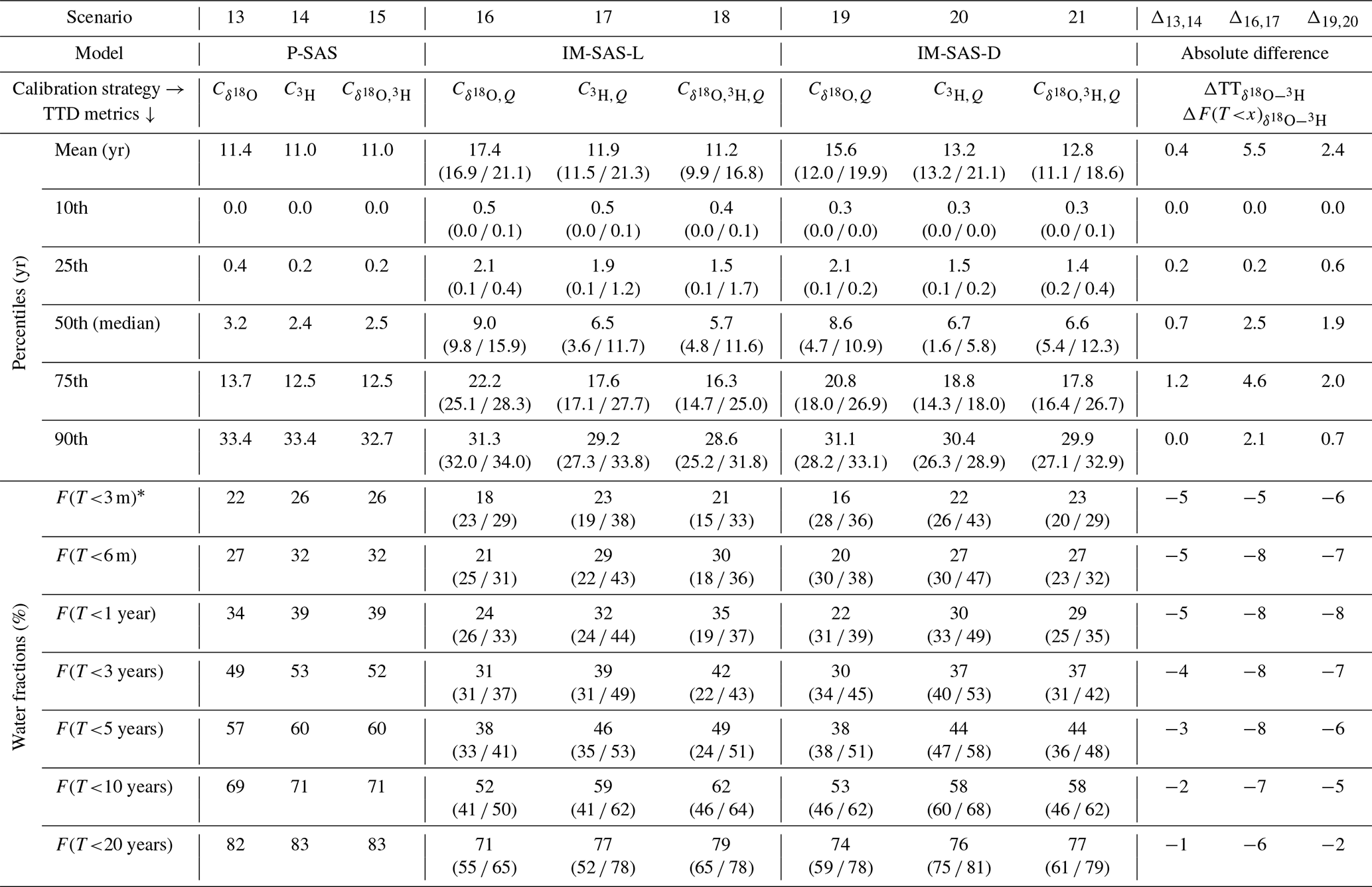
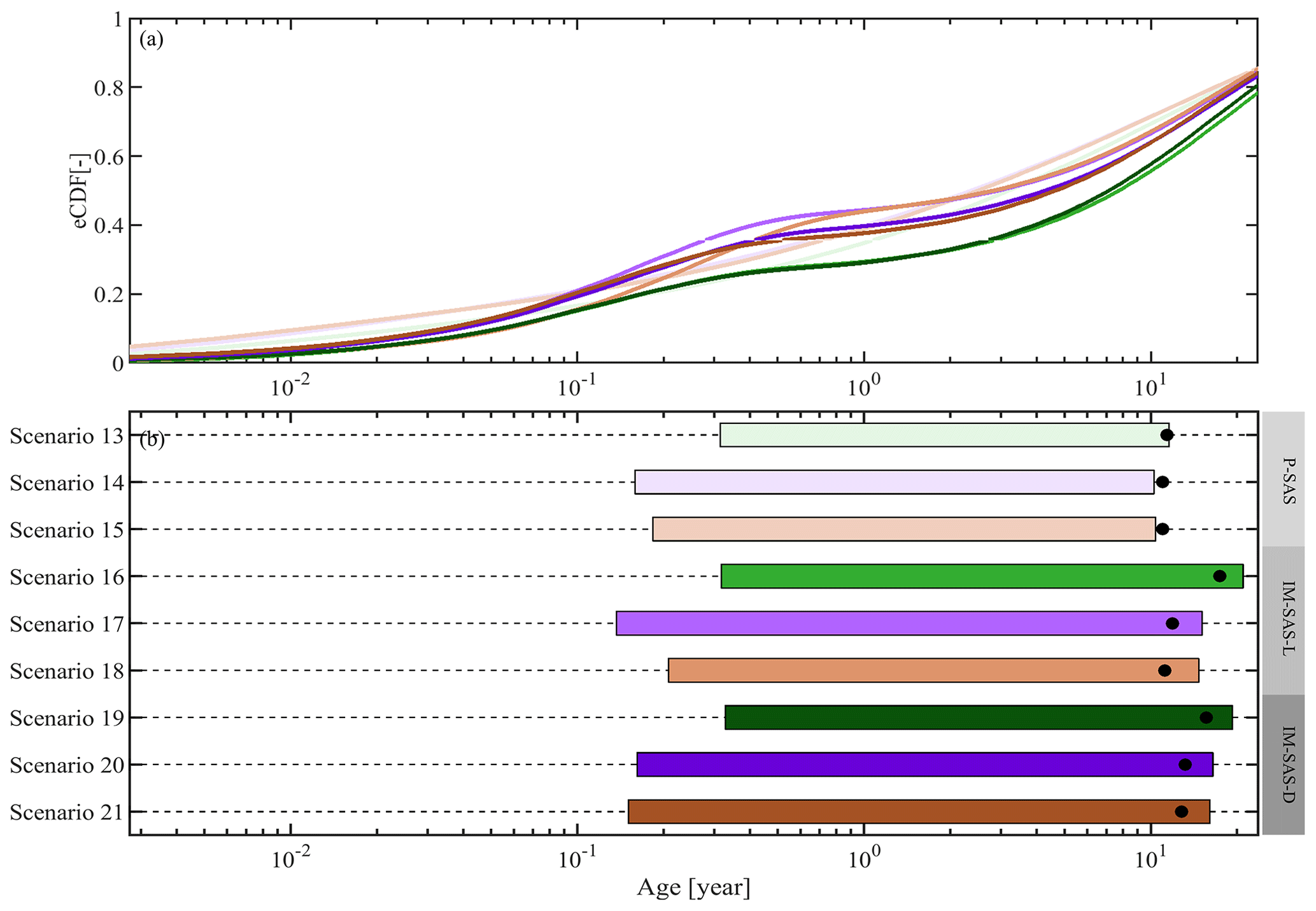
Figure 9 Streamflow TTDs derived from the nine model scenarios with the different associated calibration strategies of the P-SAS (scenarios 13–15), IM-SAS-L (scenarios 16–18) and IM-SAS-D model implementations (scenarios 19–21). The TTDs represent the volume-weighted average daily TTDs for the modelling period 1 October 2001–31 December 2016. Green shades represent the TTDs inferred from δ¹⁸O (from lighter to darker for scenarios 13, 16 and 19), the purple shades represent TTDs inferred from ³H (from lighter to darker for scenarios 14, 17 and 20), the brown lines represent TTDs inferred from combined δ¹⁸O and ³H (brown shades from lighter to darker for scenarios 15, 18 and 21), and the black dots in panel (b) indicate the mean transit time for each model scenario. Note that the mean transit time was estimated by fitting Gamma distributions to the volume-weighted mean TTDs of each individual scenario.

An explicit comparison between the lumped IM-SAS-L (scenarios 16–18) and the distributed IM-SAS-D (scenarios 19–21) also suggests a good correspondence between the respective inferred water ages for both tracers. While IM-SAS-L generates MTTs of ∼ 11.2–17.4 years, the MTT obtained from IM-SAS-D reaches ∼ 12.8–15.6 years (Table 7; Fig. 9). In addition to the MTTs, the differences in water ages across all percentiles are also minor and reach a maximum of 4.6 years at the 75th percentile. Accordingly, the fractions of water with ages T<20 years exhibit only marginal differences between the lumped (IM-SAS-L) and distributed (IM-SAS-D) model implementations. It is noted that these overall water ages from IM-SAS-D for the entire Neckar basin emerge from the aggregation of TTDs of the four individual precipitation zones P1–P4 (Figs. S29–S31 and Table S6 in the Supplement), which are characterized by pronounced differences, with MTTs ranging from ∼ 8 to 10 years in P4 and from ∼ 18 to 22 years in P2, depending on the scenario.

The consistency between water ages inferred from δ¹⁸O and ³H, respectively, in all SAS-function model scenarios is further illustrated by the direction and magnitude of change in water age distributions as a consequence of changing wetness conditions. In particular, during wet-up and wet periods, a marked variability of daily TTDs can be observed, with young water fractions F(T<3 m) ranging between ∼ 20 % and 65 % for δ¹⁸O-based estimates and between ∼ 25 % and 70% for ³H (Fig. 10a, b, e, f). Less variability in daily TTDs is found under drying and dry conditions, with F(T<3 m) generally in the range of ∼ 1 %–20 % and only a very few outliers >30 %. Overall, the volume-weighted average TTDs for wet conditions suggest slightly older water inferred from δ¹⁸O, with a median water age of ∼ 3 years and F(T<3 m) ∼ 30% for wet conditions, than from ³H, for which a median age of ∼ 1 year and F(T<3 m) ∼ 40 % were found (Fig. 10d, h). This is in contrast to dry conditions, for which the differences between δ¹⁸O- and ³H-derived water age estimates become mostly negligible (Fig. 10d, h).

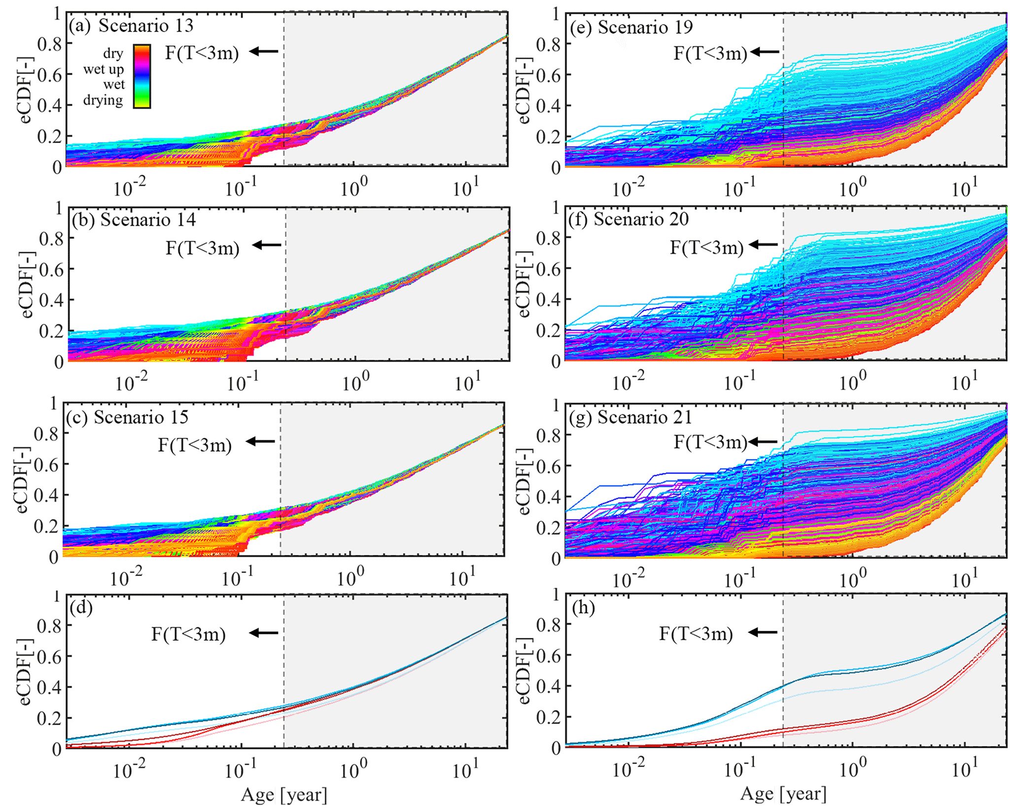
Figure 10 Daily streamflow (Q) TTDs extracted from the most balanced model solutions of P-SAS (scenarios 13–15) based on (a) calibration strategy $C_{{\mathit{\delta }}^{\mathrm{18}}\mathrm{O}}$ (scenario 13), (b) calibration strategy $C_{{}^{\mathrm{3}}\mathrm{H}}$ (scenario 14) and (c) calibration strategy $C_{{\mathit{\delta }}^{\mathrm{18}}{\mathrm{O},}^{\mathrm{3}}\mathrm{H}}$ (scenario 15), together with IM-SAS-D implementations (scenarios 19–21) based on (e) calibration strategy $C_{{\mathit{\delta }}^{\mathrm{18}}\mathrm{O},Q}$ (scenario 19), (f) calibration strategy $C_{{}^{\mathrm{3}}\mathrm{H},Q}$ (scenario 20) and (g) calibration strategy $C_{{\mathit{\delta }}^{\mathrm{18}}\mathrm{O}{,}^{\mathrm{3}}\mathrm{H},Q}$ (scenario 21). The line colours represent the transition between dry and wet periods. Panel (d) shows the volume-weighted average TTDs for the wet and dry periods, respectively. For the P-SAS model, the light shades represent calibration strategy $C_{{\mathit{\delta }}^{\mathrm{18}}\mathrm{O}}$ (scenario 13), the intermediate shades indicate calibration strategy $C_{{}^{\mathrm{3}}\mathrm{H}}$ (scenario 14), and the dark shades are calibration strategy $C_{{\mathit{\delta }}^{\mathrm{18}}{\mathrm{O},}^{\mathrm{3}}\mathrm{H}}$ (scenario 15). Panel (h) shows the volume-weighted average TTDs for the wet and dry periods, respectively. For the IM-SAS-D model, the light shades represent calibration strategy $C_{{\mathit{\delta }}^{\mathrm{18}}\mathrm{O},Q}$ (scenario 19), the intermediate shades indicate calibration strategy $C_{{}^{\mathrm{3}}\mathrm{H},Q}$ (scenario 20), and the dark shades are calibration strategy $C_{{\mathit{\delta }}^{\mathrm{18}}\mathrm{O}{,}^{\mathrm{3}}\mathrm{H},Q}$ (scenario 21). For illustrative purposes, the fraction of water younger than 3 months F(T<3 m) is also indicated.

With the P-SAS and IM-SAS models, MTTs and TTDs can be derived not only in streams, but also in any fluxes and storages (i.e. transpiration flux E_a and groundwater storage). An even more pronounced young water variability in daily TTDs was found for the transpiration flux E_a leaving the unsaturated root zone storage S_u in the IM-SAS models (scenarios 16–21). As shown in Fig. 11a, the transpiration TTDs inferred from δ¹⁸O suggest a median transpiration age during wet conditions of ∼ 2–40 d and F(T<3 m) ∼ 60 %–100 %. This variability shifts to median ages between ∼ 30 and 100 d and F(T<3 m) ∼ 30 %–95 % for dry conditions. This pattern of variability in daily TTDs in wet and dry periods is very closely matched by the estimates based on ³H (Fig. 11b). Overall, the volume-weighted average TTDs of transpiration suggest median ages of around 14 d for wet conditions and between 35 d (³H) and 70 d (δ¹⁸O) for dry conditions (Fig. 11d).

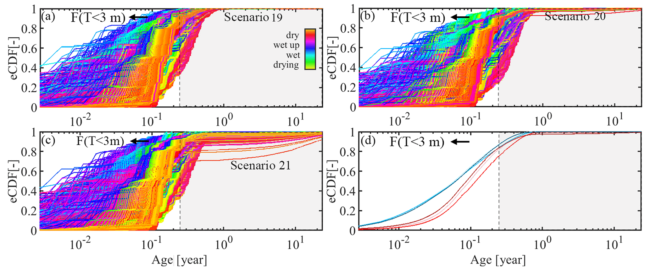
Figure 11 Daily transpiration (E_a) TTDs extracted from the most balanced model solutions of the IM-SAS-D implementations (scenarios 19–21) based on (a) calibration strategy $C_{{\mathit{\delta }}^{\mathrm{18}}\mathrm{O},Q}$ (scenario 19), (b) calibration strategy $C_{{}^{\mathrm{3}}\mathrm{H},Q}$ (scenario 20) and (c) calibration strategy $C_{{\mathit{\delta }}^{\mathrm{18}}\mathrm{O}{,}^{\mathrm{3}}\mathrm{H},Q}$ (scenario 21). The line colours represent the transition between dry and wet periods. Panel (d) shows the volume-weighted average TTDs for the wet and dry periods, respectively. The light shades represent calibration strategy $C_{{\mathit{\delta }}^{\mathrm{18}}\mathrm{O},Q}$ (scenario 19), the intermediate shades indicate calibration strategy $C_{{}^{\mathrm{3}}\mathrm{H},Q}$ (scenario 20), and the dark shades are calibration strategy $C_{{\mathit{\delta }}^{\mathrm{18}}\mathrm{O}{,}^{\mathrm{3}}\mathrm{H},Q}$ (scenario 21). For illustrative purposes, the fraction of water younger than 3 months F(T<3 m) is also indicated.

The modelled groundwater, in comparison, was found to be characterized by substantially less temporal variability in TTDs and older water ages (Fig. 12). The TTDs inferred from both δ¹⁸O and ³H are similar and are characterized by a median age of ∼ 10 years under both wet and dry conditions. While F(T<3 m) of the groundwater largely remains <1 %, around 20 %–25 % of the groundwater is older than 20 years.

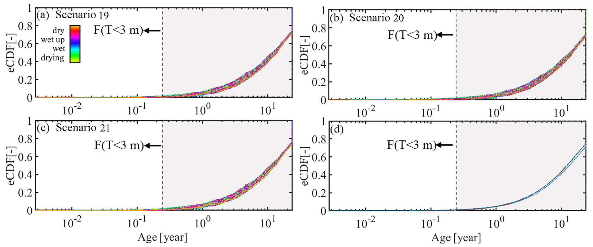
Figure 12 Daily groundwater (S_s) RTDs extracted from the most balanced model solutions of the IM-SAS-D implementations (scenarios 19–21) based on (a) calibration strategy $C_{{\mathit{\delta }}^{\mathrm{18}}\mathrm{O},Q}$ (scenario 19), (b) calibration strategy $C_{{}^{\mathrm{3}}\mathrm{H},Q}$ (scenario 20) and (c) calibration strategy $C_{{\mathit{\delta }}^{\mathrm{18}}\mathrm{O}{,}^{\mathrm{3}}\mathrm{H},Q}$ (scenario 21). The line colours represent the transition between dry and wet periods. Panel (d) shows the volume-weighted average RTDs for the wet and dry periods, respectively. The light shades represent calibration strategy $C_{{\mathit{\delta }}^{\mathrm{18}}\mathrm{O},Q}$ (scenario 19), the intermediate shades indicate calibration strategy $C_{{}^{\mathrm{3}}\mathrm{H},Q}$ (scenario 20), and the dark shades are calibration strategy $C_{{\mathit{\delta }}^{\mathrm{18}}\mathrm{O}{,}^{\mathrm{3}}\mathrm{H},Q}$ (scenario 21). For illustrative purposes, the fraction of water younger than 3 months F(T<3 m) is also indicated.

6 Implications, limitations and unresolved questions

What can we learn from the above? We believe that the results obtained in this study have several implications for the utility of different tracer and model types, as described in detail below.

6.1 The individual roles of the choices of tracers and models for underestimation of water ages

The overall magnitudes of water ages estimated here from time-invariant, lumped SW and CO models in combination with δ¹⁸O reach MTTs of ∼ 2 years (Table 6; Fig. 8). These values fall within the age ranges reported for comparable model experiments with seasonally variable tracers in many other catchments worldwide (see McGuire and McDonnell, 2006; Godsey et al., 2009; Hrachowitz et al., 2009b; Stewart et al., 2010, and references therein). Similarly, the water ages estimated with the same CO models in combination with ³H are, with MTTs of ∼ 10 years, a factor of ∼ 5 higher (Table 6; Fig. 8) and also reflect the findings of previous studies well, many of which suggest ³H-inferred catchment MTTs of ∼ 10–15 years (Stewart et al., 2010, and references therein). This suggests that the Neckar basin does not exhibit unusual or unexpected water age characteristics. By themselves, these results would therefore lend further supporting evidence for the interpretation provided by Stewart et al. (2010) and, crucially, lead us to the same conclusion that the use of δ¹⁸O and comparable seasonally variable tracers truncates stream water ages.

However, and in stark contrast, the estimates of water ages obtained from all P-SAS and IM-SAS model implementations in this study, i.e. scenarios 13–21, are similar to each other irrespective of the tracer used. Water ages estimated from δ¹⁸O are, with MTTs of >11.4 years, not only substantially older than those inferred from the SW and CO models (scenarios 1–3, 5, 7, 9 and 11), but, most importantly, are similar to those inferred from ³H in the P-SAS and IM-SAS models, which reach MTTs of ∼ 11–13 years (Table 7; Fig. 9). These water ages highlight the importance of old water in the Neckar basin, similar to what is suggested by the use of ³H in the CO models (scenarios 4, 6, 8, 10 and 12).

It is important to note that the IM-SAS and, to a lesser degree, P-SAS models can simultaneously reproduce several signatures of the hydrological response together with the δ¹⁸O and ³H stream water signals. They therefore provide a more holistic description of physical transport processes in the system (Table 7; Figs. 3–5) than the SW and CO models, which mimic one single tracer signal and thus one isolated variable at a time. In addition, the P-SAS and IM-SAS model parameters that are most linked to tracer circulation, e.g. S_tot, S_s,p and S_umax (Fig. 7), exhibit little difference when obtained from calibration to δ¹⁸O or ³H, respectively. This implies that both δ¹⁸O and ³H provide similar information about how tracers are routed through the model and how water is stored in and released from the system. As a consequence, the simultaneous representation of all three types of variables under consideration, i.e. the hydrological response as well as the δ¹⁸O and ³H stream signals, in these models is also consistent with the observed data (scenarios 18 and 21).

The above is further corroborated by how water ages in the Neckar basin respond to changing wetness conditions. Although not identical, δ¹⁸O- and ³H-inferred daily TTDs nevertheless exhibit broad agreement in the directions and magnitudes of change in response to changing wetness conditions (Fig. 10). Changes in streamflow TTDs in IM-SAS are not primarily caused by changes in water ages within individual storage components. In particular, the modelled water age distributions in the groundwater S_s show limited sensitivity to changing wetness conditions, with MTTs varying between ∼ 18 years in dry periods and ∼ 17 years in wet periods (Fig. 12). The TTDs in the transpiration flux E_a, which are reflective of the water ages in the unsaturated root zone S_u, exhibit, with MTTs of between ∼ 0.20 and 0.12 years in dry and wet periods (Fig. 11), respectively, magnitudes and fluctuations over time that are similar to what has been previously reported in other studies (e.g. Hrachowitz et al., 2015; Soulsby et al., 2016; Visser et al., 2019; Birkel et al., 2020; Kuppel et al., 2020). However, the level of these age fluctuations alone is insufficient to explain the magnitude of change in streamflow TTDs, which can vary by several years. Instead, the temporal variability of streamflow TTDs is largely controlled by switches in the relative contributions of individual storage components to streamflow under different wetness conditions. Under increasingly wet conditions, considerably increasing proportions of comparably young water from S_U contribute over shallow preferential flow pathways (S_F) to streamflow, while the relative proportion of groundwater contributing to streamflow under such conditions is reduced (Hrachowitz et al., 2013). Both tracers, δ¹⁸O and ³H, generate these patterns in a corresponding way.

Altogether, this suggests that the P-SAS and IM-SAS models and the resulting estimates of water ages inferred from both δ¹⁸O and ³H provide plausible descriptions of transport processes and thus water ages in the Neckar basin. Clearly, with current observation technology, it is impossible to know the real water age distribution at the river basin scale. However, the water ages and their temporal variability inferred from both δ¹⁸O and ³H using the P-SAS and IM-SAS models are widely consistent. This suggests that it is not the use of δ¹⁸O per se that leads to truncation of TTDs but rather that time-invariant, lumped convolution integral models are incapable of extracting sufficient information from δ¹⁸O signals. These results mirror anecdotal evidence from several previous studies (e.g. Hrachowitz et al., 2015, 2021; Ala-aho et al., 2017; Buzacott et al., 2020; Yang et al., 2021). Although no direct comparison with ³H data is provided in these studies, they demonstrated the potential of δ¹⁸O in SAS-based model approaches to estimate water age distributions with considerable fractions of water older than 5–10 years, and Birkel et al. (2020) explicitly estimated MTTs of up to 18 years. Our results also strongly support the findings and general conclusions of Rodriguez et al. (2021), who undertook a direct comparison of water ages inferred from δ¹⁸O and ³H. In their study for a small catchment based on a shorter tracer time series, i.e. 2 years, and a system that is characterized by rather low MTTs of ∼ 3 years, they found that, although ³H led to higher MTTs than δ¹⁸O, the absolute difference between these ages estimates was, at 0.2 years, limited and even decreasing for higher percentiles of the water age distributions.

We therefore argue that the evidence emerging from our results and the above considerations is strong enough to reject the hypothesis that δ¹⁸O as a tracer generally and systematically “cannot see water older than about 4 years” (Stewart et al., 2010, 2012) and the corresponding tails in water age distributions, leading to underestimations of water ages. We further argue that previous underestimations of water ages are rather a consequence of the use of time-invariant, lumped-parameter convolution integral model techniques that cannot resolve the information contained in δ¹⁸O signals in a meaningful way for catchments with transient flow conditions. In contrast, the combined information using hydrological and tracer data and thus the consideration of transient flow conditions results in similar MTTs, independent of the tracer used. Note that, for this reason, time-variant implementations of convolution integral models that can describe transient conditions may hold the potential to similarly generate water age estimates from δ¹⁸O signals that reflect the results of the P-SAS and IM-SAS models tested here.

However, and notwithstanding the rejection of the above hypothesis, it is important to note that overall, and in spite of the similarity between δ¹⁸O- and ³H-inferred water ages in the study basin on the basis of the P-SAS and IM-SAS models, there may be no general equivalence between δ¹⁸O and ³H tracers. Instead, it is plausible to assume that differences will gradually increase with higher water ages. In systems characterized by water older than the water in the Neckar study basin and where the amplitudes of the δ¹⁸O stream signal are attenuated to below the analytical precision, the water age estimates from δ¹⁸O will indeed become subject to increasing uncertainty up to the point where further attenuation and thus older water ages cannot be discerned anymore, independent of modelling approaches. The specific magnitude of such a water age threshold remains difficult to quantify with the available data. However, given the results in the Neckar study basin, the question raised by Stewart et al. (2021), whether δ¹⁸O allows one to see “the full range of travel times”, can to some extent be answered: it can be assumed that, when used with a suitable model, δ¹⁸O contains sufficient information for a meaningful characterization of water ages in systems characterized by MTTs of at least ∼ 15–20 years, which encompasses the vast majority of river basins analysed so far in the literature (see Stewart et al., 2010, and references therein). As a step forward, the original hypothesis above can, for future research, be reformulated: δ¹⁸O-inferred water age estimates are subject to increasing uncertainty and bias when compared to ³H-inferred estimates when stream water MTTs of ∼ 15–20 years are exceeded in systems characterized by increasingly old water.

6.2 The role of spatial aggregation in underestimation of water ages

In addition to the above, Kirchner (2016) demonstrated that the use of seasonally variable tracers with time-invariant, lumped-parameter model approaches, i.e. SW and CO, has considerable potential to underestimate water ages due to spatial aggregation of heterogeneous MTTs in systems characterized by large spatial contrasts in MTTs. We could not reproduce that exact experiment here, as stream observations were only available at one location for each tracer. However, in the distributed implementation of the IM-SAS-D model (scenarios 19–21), we nevertheless explicitly accounted, albeit to a limited degree, for heterogeneity in the system input variables and for potential differences in landscape types, as expressed by the three model HRUs. This resulted in different TTDs for the individual precipitation zones (Figs. S29–S31 and Table S6 in the Supplement), elevation zones and HRUs therein (not shown). The comparison between the lumped IM-SAS-L (scenarios 16–18) and distributed IM-SAS-D models does not show major differences in their ability to reproduce the various hydrological signatures or the δ¹⁸O and ³H stream signals (Table 5). Against evidence from various previous studies (e.g. Euser et al., 2015; Gao et al., 2016; Nijzink et al., 2016; Nguyen et al., 2022), this reflects to some degree the conclusion by Loritz et al. (2021), who found in a comparative analysis that distributed model implementations do not necessarily improve a model's ability to reproduce the hydrological response as compared to spatially lumped formulations. In addition, the contrasts in water ages between the discretized model components, with MTTs ranging from ∼ 8 to ∼ 22 years in the individual precipitation zones, may not be sufficient to significantly affect overall basin MTTs. As a consequence, the results of IM-SAS-L and IM-SAS-D also do not show major differences in the associated water age estimates, with MTTs of ∼ 11–17 years and 12–16 years, respectively (Table 7; Fig. 9).

How can this be interpreted? If significantly older ages were inferred from the distributed IM-SAS-D implementation, this would have provided strong supporting evidence for the role and effect of spatial heterogeneity on water ages as demonstrated by Kirchner (2016). However, the similar water ages inferred from the spatially lumped and distributed implementations, respectively, allow two possible but mutually contradictory interpretations. They could indicate either that the aggregation of spatial heterogeneity does not have any discernible effect on water ages inferred from the IM-SAS model in the study basin or, by contrast, that the spatial contrasts in water ages, limited by the spatial resolution of the model and the available data, were not sufficient to detect any significant differences. The evidence found here therefore remains inconclusive, and further research is required to describe the role of the aggregation of spatial heterogeneity in estimates of water ages using the IM-SAS type of model.

For any estimates of water ages in this study – as in any other study – it is important to bear in mind that they are conditional on the available data and models used. Uncertainties can and do arise from both data and decisions made in the modelling process (e.g. Beven, 2006; Kirchner, 2006). One challenge in this study was that precipitation δ¹⁸O and ³H compositions were only available at rather coarse spatial and temporal resolutions. We have used the best-available information to spatially extrapolate the tracer precipitation data from the individual sampling stations in order to estimate their spatial variation across the Neckar basin, including stations outside the study basin. The monthly δ¹⁸O and ³H distribution in precipitation within southern Germany is generally similar (Stumpp et al., 2014; Schmidt et al., 2020); still, regional correction for δ¹⁸O might not be sufficient to explain local differences in δ¹⁸O precipitation data. A similar limitation applies to the temporal resolution of tracer composition in precipitation as only monthly information was available. However, as the available data nevertheless reflect the seasonal variation in δ¹⁸O and ³H precipitation input, the uncertainties arising can be assumed to largely affect the short-term dynamics of tracers in the stream and thus rather young water ages, whereas the objective of our analysis was focused on the right tail of the water age distributions and thus on old ages. Notwithstanding these uncertainties, the overall model performances with respect to the hydrological and tracer responses suggest that the choice of input data and the model formulations led to model results that are largely consistent with the observed responses in the stream. The observation that there is little ambiguity in the results further suggests that the remaining uncertainties are unlikely to affect the overall interpretation and conclusions of this study.

7 Conclusions

δ¹⁸O and ³H are frequently used as tracers in environmental sciences to estimate age distributions of water. However, it has previously been argued that seasonally variable tracers, such as δ¹⁸O, fail to detect the tails of water age distributions and therefore substantially underestimate water ages as compared to radioactive tracers such as ³H. In this study for the Neckar River basin in central Europe and based on a > 20-year record of hydrological, δ¹⁸O and ³H data, we systematically scrutinized the above postulate by comparing water age distributions inferred from δ¹⁸O and ³H with a total of 21 different model implementations. The main findings of our analysis are the following.

1. Water ages inferred from δ¹⁸O with commonly used time-invariant, sine-wave (SW) and lumped-parameter convolution integral models (CO) are, with MTTs of ∼ 1–2 years, substantially lower that those obtained from ³H with the same models, reaching MTTs of ∼ 10 years.

2. In contrast, the concept of SAS functions in combination with hydrological models (P-SAS, IM-SAS) not only allowed simultaneous representations of water storage fluctuations together with δ¹⁸O and ³H stream signals, but water ages inferred from δ¹⁸O were, with MTTs of ∼ 11–17 years, much higher and even higher than inferred from ³H, which suggested MTTs of ∼ 11–13 years.

3. Constraining P-SAS and IM-SAS model implementations individually with δ¹⁸O and ³H observations resulted in similar values for parameters that control water ages, such as the total storage S_tot (P-SAS) or passive groundwater volumes S_s,p (IM-SAS). In addition, δ¹⁸O- and ³H-constrained models both exhibited limited differences in the magnitudes of water ages in different parts of the models as well as in the temporal variability of TTDs in response to changing wetness conditions. This suggests that both tracers lead to comparable descriptions of how water is routed through the system.

4. Based on the points above, we reject the hypothesis that δ¹⁸O as a tracer generally and systematically “cannot see water older than about 4 years” (Stewart et al., 2010, 2012) and that it truncates the corresponding tails in water age distributions, leading to underestimations of water ages.

5. Instead, our results provide evidence for broad equivalence of δ¹⁸O and ³H as age tracers for systems characterized by MTTs of at least 15–20 years.

6. The question of the degree to which aggregation of spatial heterogeneity can further adversely affect estimates of water ages remains unresolved as the lumped and distributed implementations of the IM-SAS model provided similar and thus inconclusive results.

Overall, this study demonstrates that previously reported underestimations of water ages are most likely not a result of the use of δ¹⁸O or other seasonally variable tracers per se. Rather, these underestimations can be largely attributed to the choices of model approaches which rely on assumptions not frequently met in catchment hydrology. Given the vulnerability of lumped, time-invariant parameter convolution integral approaches in combination with δ¹⁸O to substantially underestimate water ages due to transient flow conditions, spatial aggregation and potentially other, still unknown effects, we therefore strongly advocate avoiding the use of this model type in combination with seasonally variable tracers and instead adopting SAS-based or other model formulations that allow for the representation of transient conditions.