Technical note: Lessons from and best practices for the deployment of the Soil Water Isotope Storage System

Soil water isotope datasets are useful for understanding connections between the hydrosphere, atmosphere, biosphere, and geosphere. However, they have been underproduced because of the technical challenges associated with collecting those datasets. Here, we present the results of testing and automation of the Soil Water Isotope Storage System (SWISS). The unique innovation of the SWISS is that we are able to automatically collect water vapor from the critical zone at a regular time interval and then store that water vapor until it can be measured back in a laboratory setting. Through a series of quality assurance and quality control tests, we tested whether the SWISS is resistant to both atmospheric intrusion and leaking in both laboratory and field settings. We assessed the accuracy and precision of the SWISS through a series of experiments in which water vapor of known composition was introduced into the flasks, stored for 14 d, and then measured. From these experiments, after applying an offset correction to report our values relative to Vienna Standard Mean Ocean Water (VSMOW), we assess the precision of the SWISS to be ±0.9 ‰ and ±3.7 ‰ for δ¹⁸O and δ²H, respectively. We deployed three SWISS units at three different field sites to demonstrate that the SWISS stores water vapor reliably enough that we are able to differentiate dynamics both between the sites as well within a single soil column. Overall, we demonstrate that the SWISS retains the stable isotope composition of soil water vapor for long enough to allow researchers to address a wide range of ecohydrologic questions.

1 Introduction

Understanding soil water dynamics across a range of environments and soil properties is critical to food and water security (e.g., Mahindawansha et al., 2018; Quade et al., 2019; Rothfuss et al., 2021); understanding biogeochemical cycles, such as the nitrogen and phosphorus cycles (e.g., Hinckley et al., 2014; Harms and Ludwig, 2016); and understanding connections between the hydrosphere, biosphere, geosphere, and atmosphere (e.g., Vereecken et al., 2022). One approach that can be used to understand water use and movement in the critical zone is the stable isotope geochemistry of soil water (e.g., Sprenger et al., 2016; Bowen et al., 2019). Variations in the stable isotope ratios of oxygen and hydrogen of soil water (δ¹⁸O, δ²H) track physical processes like infiltration, root water uptake, and evaporation. In particular, stable water isotopes are useful for disentangling complex mixtures of water from multiple sources (e.g., Dawson and Ehleringer, 1991; Brooks et al., 2010; Soderberg et al., 2012; Good et al., 2015; Bowen et al., 2018; Gómez-Navarro et al., 2019; Sprenger and Allen, 2020). Despite the long-recognized utility of measuring soil water isotopes for understanding a range of processes (e.g., Zimmermann et al., 1966; Peterson and Fry, 1987), soil water isotope datasets have been underproduced compared with groundwater and meteoric water isotope datasets (Bowen et al., 2019).

The primary barrier to producing soil water isotope datasets has been the arduous nature of collecting samples. Historically, there are two primary methods for collecting soil water samples: either digging a pit and collecting a mass of soil to bring back to the lab for subsequent water extraction or collecting samples via lysimeter. The former method disrupts the soil profile each time that a sample is collected, inhibiting the creation of long-term records of soil water isotopes. Lysimeters, on the other hand, provide the means to collect multiyear soil water isotope datasets (e.g., Stumpp et al., 2012; Zhao et al., 2013; Hinckley et al., 2014; Green et al., 2015; Groh et al., 2018), but the choice of lysimeter can affect the portion of soil water (i.e., mobile vs. bound) that is sampled (Hinckley et al., 2014; Sprenger et al., 2015) and the soil conditions that are able to be sampled (i.e., saturation state). Soil water samples collected from both bulk soil samples and lysimeters often require manual intervention at the time of sampling.

Building off of innovations in laser-based spectroscopy for stable isotope geochemistry, the ecohydrology community has developed a variety of in situ soil water sampling methods over the last 15 years that have enabled the creation of high-throughput, high-precision analyses of soil water isotopes (e.g., Wassenaar et al., 2008; Gupta et al., 2009; Rothfuss et al., 2013; Volkmann and Weiler, 2014; Gaj et al., 2016; Oerter et al., 2016; Beyer et al., 2020; Kübert et al., 2020). These methods have provided insights into a range of ecohydrologic questions from evaporation and water use dynamics in managed soils (e.g., Oerter and Bowen, 2017; Quade et al., 2018) to better understanding where plants and trees source their water (e.g., Beyer et al., 2020). These innovations have allowed researchers to ask new questions about ecohydrologic dynamics, but current methods require field deployments of laser-based instruments. Field deployments are technically possible and have been conducted successfully (e.g., Gaj et al., 2016; Volkmann et al., 2016; Oerter and Bowen, 2017; Quade et al., 2019; Kühnhammer et al., 2022; Seeger and Weiler, 2021; Gessler et al., 2022), but they require uninterrupted alternating-current (AC) power, adequate shelter, and safe and stable operating environments for best results. These prerequisites are often unavailable at many field sites, especially at more remote locations and for longer sampling time frames. Given these logistical constraints, these studies have mostly been done near the institutions performing those studies. Spatial constraints limit the questions that researchers can ask about soil hydrology in remote and traditionally understudied landscapes. For example, in the geoscience community, there is significant interest in improving the research community's understanding of how and when paleoclimate proxies (stable isotope records from pedogenic carbonate, branched glycerol dialkyl glycerol tetraethers, etc.) form in soils, because that informs our ability to accurately interpret records from the geologic past. However, those projects commonly have environmental constraints, like soil type or local climate characteristics, that may not be located near the institutions performing those studies. To be able to study a broader range of questions about ecohydrology, there is a need for a system that is capable of autonomously collecting soil water vapor for isotopic analysis in remote settings.

In this contribution, we report on the further development and testing of a field-deployable system called the Soil Water Isotope Storage System (SWISS). The SWISS was built to be paired with ACCUREL PP V8/2HF vapor-permeable probes that have been previously tested for soil water isotope applications (Rothfuss et al., 2013; Oerter and Bowen, 2017). Our system uses three basic components to store water vapor produced by the vapor-permeable probes: glass flasks, stainless-steel tubing, and a flask selector valve (Fig. 1, Table S1). Previously, through a series of lab experiments, we demonstrated that the glass flasks used in the SWISS units can reliably store water vapor for up to 30 d (Havranek et al., 2020). That proof-of-concept study demonstrated that the flasks retain original water isotope values, but the laboratory system was not field deployable and did not have customizable automation. Here, we present a fully autonomous, field-ready system that has been tested under both laboratory conditions and field conditions, including development and testing of a solar-powered, battery-backed automation system that enables pre-scheduled water vapor sampling without manual intervention in remote field locations.

To test the accuracy and precision of the SWISS, we completed QA/QC tests. Here, we demonstrate the viability of this system under field conditions through two field suitability experiments. In addition, we sampled three different field sites to show that the automation schema works on a monthly timescale and that the system preserves soil water vapor isotope signals with sufficient precision to distinguish between three different field settings and vertical profile differences.

2 Field sites

2.1 Site setup

At each site, we dug two holes; Fig. 1 shows the field setup employed at all of our field sites. One hole was instrumented with soil moisture and temperature data loggers at 25, 50, 75, and 100 cm depths as well as water-vapor-permeable probes at 25, 50, and 75 cm depths (Fig. 1a). We deployed all probes > 9 months before the first samples were collected to allow the soil to settle and return to natural conditions as much as possible. This time frame was longer than other studies (e.g., Kübert et al., 2020) and included the infiltration of spring and early-summer precipitation. During probe deployment, we took care to retain the original soil horizon sequence and horizon depths as much as possible. In the second hole, we stored the SWISS unit, a dry-nitrogen tank, and associated components to power the SWISS (Fig. 1b). The water vapor probes, which were connected to the SWISS units with Bev-A-Line impermeable tubing, were run through a PVC pipe buried at approximately 15 cm depth. We ran the impermeable tubing underground to limit the effect of diurnal temperature variability on the impermeable tubing to prevent condensation as water travels from the relatively warm soil to the SWISS.

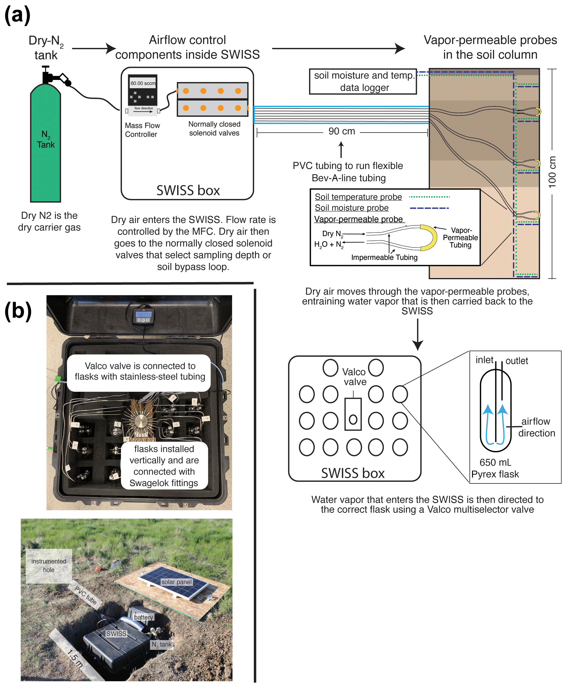
Figure 1 (a) The sampling flow path. To sample soil water, dry nitrogen is regulated at a specific rate using a mass flow controller and then directed to one of the three sampling depths or to the soil bypass loop using a set of solenoid valves. Both the mass flow controller and solenoid valves are housed inside the SWISS. Once directed to the correct sampling depth, dry nitrogen is carried to the vapor-permeable probes via gas-impermeable tubing that is buried at approximately 15 cm depth. After passing through the vapor-permeable probe, the entrained soil water vapor is carried back to the SWISS where it is directed to the correct flask using a Valco multi-selector valve. (b) Photos of a built-out SWISS and the layout of a field site. Each of the system components (solar panel, battery, N₂ tank, SWISS, PVC tube) and the location of the instrumented hole in which all of the probes are buried are labeled. The hole that houses the SWISS, power, and N₂ tank is approximately 1.5 m wide.

2.2 Site descriptions

We deployed the SWISS at three field locations: Oglala National Grassland, Nebraska, USA; Briggsdale, Colorado, USA; and Seibert, Colorado, USA. The Oglala National Grassland site (lat 42.9600, long −103.5979; elevation 1117 m) is located in northwestern Nebraska, USA, in a cold, semiarid climate. The soil at this site is described as an Aridisol with a silt loam texture. It is part of the Olney series (Soil Survey Staff et al., 2022). The Briggsdale site (lat 40.5947, long −104.3190; elevation 1480 m) is located in northeastern Colorado, USA, in a cold, semiarid climate. The soil at this site is described as an Alfisol with a loamy sand–sandy loam texture. It is part of the Olnest series (Soil Survey Staff et al., 2022). Long-term meteorological data from the Briggsdale site are available from the co-located Colorado Agricultural Meteorological Network (CoAgMet) site (CoAgMet, 2023). The Seibert site (lat 39.1187, long −102.9250; elevation 1479 m) is located in eastern Colorado, USA, in a cold, semiarid climate. The soil at this site has been described as an Alfisol that has a sandy loam texture in the top 50 cm of the profile and a silt loam texture between 50 and 100 cm. It is part of the Stoneham series (Soil Survey Staff et al., 2022). Long-term meteorological data from the site are available from the co-located CoAgMet site (CoAgMet, 2023).

3 Materials

3.1 SWISS hardware components

In each SWISS there are 15 custom-made ∼650 mL flasks. These flasks are designed similarly to those used for other water vapor applications. For example, a similar flask is currently used in a UAV to collect atmospheric water vapor samples for stable isotope analysis (Rozmiarek et al., 2021). The flasks have one long inlet tube that extends into the flask almost to the base and one shorter outlet tube so that vapor exiting the flask is well mixed and representative of the whole flask (Fig. 1a). The large flask volume is advantageous because there is a low glass-surface-area-to-volume ratio; therefore, we are able to reliably measure vapor from the flasks on a cavity ring-down spectroscopy (CRDS) instrument without interacting with vapor bound to the flask walls. The 15 glass flasks are connected to a 16-port multi-selector Valco valve (Valco Instruments Co. Inc.). We chose to use a Valco valve because these have previously been shown to sufficiently seal off sample volumes for subsequent stable isotope analysis (Theis et al., 2004). The valve and flasks are connected by $\mathrm{1}/\mathrm{8}$ in. stainless-steel tubing and $\mathrm{1}/\mathrm{4}$ to $\mathrm{1}/\mathrm{8}$ in. stainless-steel union Swagelok fittings (Swagelok Co.); we use PTFE ferrules on the glass flasks with the Swagelok fittings. The first port of the Valco valve is $\mathrm{1}/\mathrm{8}$ in. stainless-steel tubing that serves as a flask bypass loop, enabling the flushing of either dry air or water vapor through the system without interacting with a flask. All components are contained in a 61 cm × 61 cm × 61 cm Pelican case (Pelican 0370) with three layers of Pick N Pluck foam and convoluted foam (Pelican Products Inc.). This case is thermally insulated and provides enough protection to safely transport the SWISS by vehicle to field sites.

3.2 Soil probes

There are three components for the collection and analysis of soil water vapor: vapor-permeable probes, soil temperature loggers, and soil moisture sensors (Fig. 1b, Table S1).

Here, we use a vapor-permeable membrane (ACCUREL PP V8/2HF, 3M) that was first tested for soil water isotope applications by Rothfuss et al. (2013). This method works by flushing dry nitrogen (or dry air) through the vapor-permeable membrane, creating a water vapor concentration gradient from inside the probe to the soil, thus inducing water vapor movement across the membrane. Water vapor is then entrained in the dry nitrogen and flushed to either a CRDS system or into a storage container. We opted to use this tubing because it has been shown to deliver reliable data over time (i.e., Rothfuss et al., 2015; Oerter and Bowen, 2019; Kübert et al., 2020; Seeger and Weiler, 2021; Gessler et al., 2021), it is easy to use, and it can be customized to individual needs (Beyer et al., 2020; Kübert et al., 2020). We previously observed that variability in the length of the vapor-permeable tubing can lead to systematic offsets in the stable isotope composition of measured waters that arise from variability in the vapor-permeable tube surface area (Havranek et al., 2020). Therefore, we were careful to construct all probes such that the length of the ACCUREL vapor-permeable tubing was 10 cm long and the impermeable Bev-A-Line IV connected on each side of the vapor-permeable tubing was 2 m long. We cut the Bev-A-Line connections to identical lengths to control for memory effect and to treat all samples identically. We also constructed the vapor-permeable probes to be used in the lab setting for standards in an identical fashion.

Soil temperature loggers (Onset Computer Corp., Hobo MX2201), used for applying a temperature correction to all soil water vapor data and to provide key physical parameters of the soils for other goals beyond this study, were buried at the same depths as the vapor-permeable probes. Soil moisture sensors (Onset Computer Corp., S-SMD-M005) were also buried at the same depths as the vapor-permeable probes.

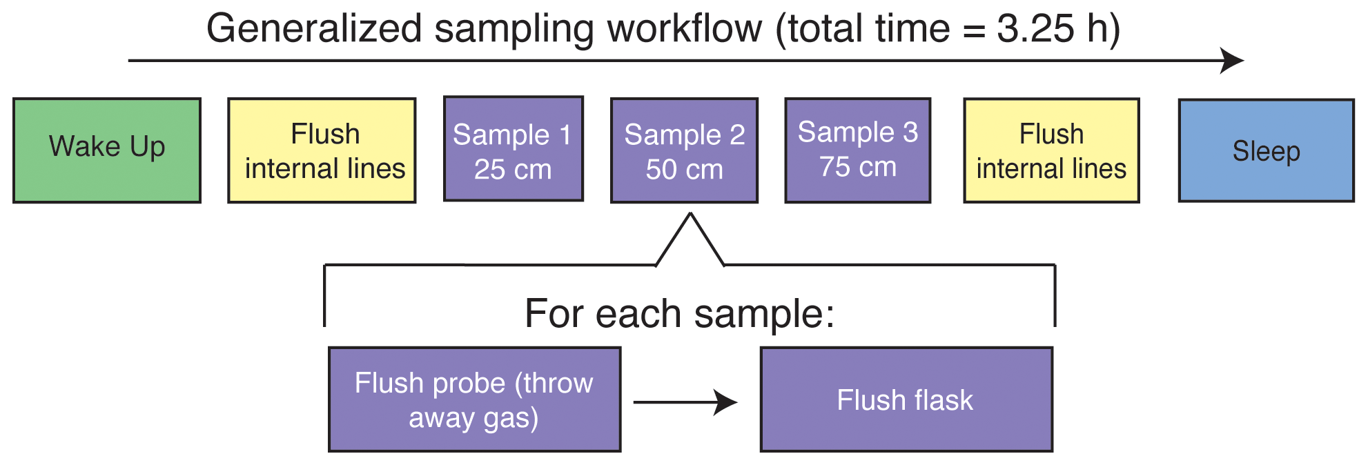
Figure 2 Flow chart of the instrument schedule used for sampling during all field experiments.

Table 1 Description of soil water sampling steps.

3.3 Automation components, code style, and power in a remote setting

The philosophy behind the automation of the SWISS was to make it as easy to reproduce as possible and as flexible as possible to meet different users' sampling needs. Therefore, we use widely available hardware components and electronics parts; for each product there are numerous alternatives that should be equally viable and could be swapped to better meet each user's needs. In an effort to make our system as accessible and customizable as possible for the scientific community, all automation code is completely open source and will continue to be refined for future applications and hardware improvements. We note that all code is provided “as is” and should be tested carefully for use in other experiments.

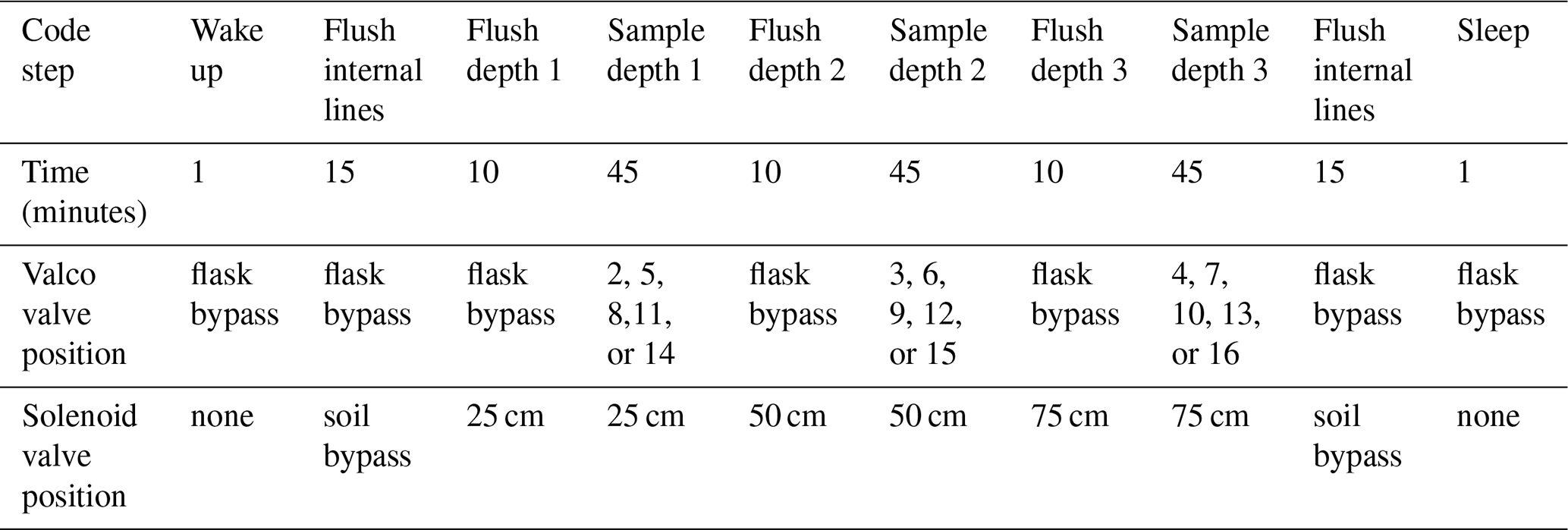
The overall sampling scheme used in this paper is described in Fig. 2 and Table 1. Our experimental goal was to create a time series of soil water vapor data from three discrete sampling depths (25, 50, and 75 cm). Prior to sampling any soil water vapor, we bypassed the soil probes and flushed the lines within the SWISS. Then, at the start of sampling for each depth, we also flushed the water vapor probe to remove condensation or “old” water vapor. The gas from both of those steps was expelled via the flask bypass loop. Each soil depth was then sampled for 45 min by flushing through the next flask designated in the sequence.

Figure S1 in the Supplement shows the components of the automation system. To automate and program the sampling scheme, we used the following: (1) a microcontroller to run the automation script; (2) a coin-cell battery-powered real-time clock so that the microcontroller was always capable of keeping track of time through power losses and, therefore, maintain the sampling schedule; (3) a Recommended Standard 232 (RS-232) to transistor–transistor logic (TTL) converter for serial communication with the Valco valve; (4) solenoid valves that were used to control which depth was being sampled and the associated volt-direct-current (VDC) power relay; (5) a mass flow controller used to control the rate at which dry nitrogen (1 ppm H₂O) was flushed through the probes; and (6) a power relay used to power the Valco valve and mass flow controller. All parts are described in detail in Table S2.

In a remote setting, the SWISS units are powered using the combination of a 12 V deep-cycle battery with a 12 VDC, 100 W solar panel that is used to charge the battery. The solar panel is mounted to a piece of plywood that covers the hole where the SWISS is deployed (note that the hole is uncovered in Fig. 1b for illustrative purposes). We opted for this setup because the underground storage of all parts of the system creates a discreet field site that attracts minimal attention from other land users and helps reduce exposure to temperature and precipitation extremes. In the field, we used a 12 VDC–120 VAC (volt-alternating-current) power inverter to provide simple plug-and-play power for the Valco valve and mass flow controller. This simple combination was suitable for summertime in the western USA, which experiences many hours of direct sunlight, and the solar panel was able to easily charge the 12 V battery. This setup may need to be adjusted based on location and desired sampling time. Like the automation system, there are many commercial options available for products, and they can be easily adjusted to users' needs; example parts are described in detail in Table S2. We also note that the deep-cycle battery, solar panel, and power inverter can be removed in areas where it is possible to plug into a power grid.

4 Methods

We completed all water vapor isotope analyses at the Stable Isotope Lab, Institute of Arctic and Alpine Research (INSTAAR SIL), located at the University of Colorado Boulder, between October 2020 and August 2022. We used a Picarro L2130-i water isotope analyzer (Picarro Inc.) to measure both water concentration and the oxygen and hydrogen isotope ratios of the water vapor.

4.1 Quality assurance and quality control (QA/QC): testing the SWISS under lab conditions

Our highest-order concern for the SWISS is that it remains leak-free, as leaks would introduce the potential for fractionation or mixing with atmosphere that would alter the stable isotope ratio of the water vapor in the flask. To mitigate leaks, we developed a three-part QA/QC procedure that must be completed for each new SWISS prior to the first deployment. The first step detects any large, fast leaks using helium detection methods; the second step detects medium-scale leaks using dry air; and the third step detects slow, small-scale leaks using water vapor tests. Full procedural descriptions are available in the Supplement, and the data processing code is available via GitHub.

4.1.1 Step 1: use helium to detect large, fast leaks

After the initial assembly of the SWISS units, we looked for large leaks from the cracking of inlet or outlet tubes on the glass flasks that occasionally occurred while tightening the Swagelok fittings. To do this, we filled the flasks with helium and used a helium leak detector (Leak Detector, catalog no. 22655, Restek). Another easy alternative to a helium leak test is to complete a very short dry-air test (methods described below) where the hold time is on the order of 12–24 h.

4.1.2 Step 2: use dry air to detect medium-scale leaks

The goal of this test was to catch any second-order, medium-scale leaks associated with either Valco valve fittings or Swagelok fittings that were under-tightened.

Step 2A: fill flasks with dry air

To start every experiment, we filled flasks with air that had been filtered through Drierite (which has a water vapor mole fraction of less than 500 ppm) at 2 L min⁻¹ for 5 min. With a flask volume of 650 mL, this meant that the volume of the flask was turned over 15 times.

Step 2B: hold period

Flasks were then sealed and left to sit for 7 d. This time period can be adjusted by other users to fit their climate or needs.

Step 2C: measure water vapor mole fraction using dead-end pull sample introduction

At the end of the 7 d period, we measured each flask using a dead-end pull sample introduction method. For this sample introduction method, the inlet to the Valco valve was sealed with a $\mathrm{1}/\mathrm{4}$ in. Swagelok cap and there was no introduction of a carrier gas. As a result, air was removed from the flask based on the flow rate of the Picarro analyzer (typically 27–31 mL min⁻¹). Flasks were measured for 5 min, which resulted in ∼150 mL of air being removed from the flasks. All components within the SWISS are capable of being fully evacuated. Water vapor mole fractions determined by Picarro instruments are not standardized, so it is impossible to know for sure the exact magnitude of the water vapor mole fraction change between the input analysis and the final value at the end of the dry-air test. However, these instruments are remarkably stable over weeks; therefore, the relative changes observed (e.g., increase or decrease in the mole fraction relative to the initial amount) are likely reliable, particularly for the larger-magnitude changes.

If a flask had a water vapor mole fraction of less than 500 ppm, it “passed” Step 2 of QA/QC. If a flask had a water vapor mole fraction greater than 500 ppm, it “failed” Step 2 of QA/QC, and we tightened both the Swagelok connections on the flasks as well as the fittings between the stainless-steel tubing and the Valco valve. We repeated dry-air tests on any given SWISS unit until the majority (typically at least 13 of 15) of the flasks had passed Step 2 of QA/QC.

4.1.3 Step 3: water vapor tests detect small-scale leaks

The purpose of this experiment was to mimic the storage of water vapor at concentrations similar to what we might expect in a soil and for durations similar to those of our field experiments. These experiments were meant to test whether flasks filled early in the sampling sequence during field deployments leak by the time samples are returned to the lab for measurement. For this experiment, we filled flasks with water vapor of known isotopic composition and water vapor mole fraction, sealed the flasks for 14 d, and then measured the water vapor mole fraction and isotope values of each flask. We performed 11 water vapor tests that were done across three analytical sessions using six different SWISS units. Across these three sessions, we measured 164 flasks, both at the start of the 14 d experiment and at the end.

Step 3A: flush flasks with dry air

Prior to putting any water vapor into the flasks (either in the field or in the lab), we completed a dry-air fill (as described in QA/QC Step 2A) that served to purge the flasks of any prior water vapor that might exchange with the new sample.

Step 3B: fill flasks with water vapor and measure the input isotope values

To supply water vapor to the flasks, we used the vapor-permeable probes that were constructed identically to those deployed in the field. We immersed the probes up to the connection between the vapor-permeable and -impermeable tubing in water, taking care to not submerge the connection point and inadvertently allow liquid water to enter the inside of the vapor-permeable tubing. We flushed the flasks at a rate of 150 mL min⁻¹ for 30 min and then measured the δ¹⁸O and δ²H values and the mole fraction of water vapor as each flask was filled. To fill 15 flasks sequentially, the probes were submerged in water for approximately 7.5 h.

Across three different sessions, we used three different waters that are tertiary standards at the INSTAAR SIL to complete these experiments: a light water made by melting and filtering Rocky Mountain snow ($\sim -\mathrm{25.5}$ ‰ and −187.5 ‰ VSMOW for δ¹⁸O and δ²H, respectively), an intermediate water that is deionized (DI) water from the University of Colorado Boulder Campus ($\sim -\mathrm{16.2}$ ‰ and −120.7 ‰ VSMOW for δ¹⁸O and δ²H, respectively), and a heavy water that is filtered water sourced from Florida, USA ($\sim -\mathrm{0.8}$ ‰ and −2.8 ‰ VSMOW for δ¹⁸O and δ²H, respectively). All tertiary lab standards are characterized relative to international primary standards obtained from the International Atomic Energy Agency and are reported relative to the VSMOW/SLAP standard isotope scale. To calculate the input value, we averaged δ¹⁸O and δ²H values over the last 3 min of the filling period. We then stored the water vapor in the flasks for 14 d. At the end of the 14 d storage period, we measured each flask to evaluate if the δ¹⁸O and δ²H values had significantly changed over the storage period.

Step 3C: measure the water vapor isotope values

To mitigate the memory effects between flasks, we ran dry air via the flask bypass loop (port 1 of every SWISS unit) for 5 min between each flask measurement. To verify that the impermeable tubing between the SWISS and the Picarro instrument was sufficiently dried, we waited until the water vapor mixing ratio being measured by the Picarro instrument was below 500 ppm for >30 s.

During this 5 min window, we used a heat gun to manually warm each flask. We believe that heating the flasks creates a more stable measurement by limiting water vapor bound to the glass walls of the flask and by helping to homogenize the water vapor within the flask. While we did not strictly control or regulate the temperature of the flasks, they were all warm to the touch.

Once we warmed the flask and dried the impermeable tubing, water vapor was introduced to the CRDS using one of two methods: (1) the dead-end pull sample introduction method described above or (2) a dry-air carrier-gas sample introduction method. During the dry-air carrier-gas sample introduction method, dry air is continuously flowing through the flask at a rate of 27–31 mL min⁻¹ for the entire 12 min measurement period. To reach a water vapor mole fraction of approximately 25 000 ppm (the optimal humidity range for the Picarro L2130-i), we diluted the water vapor with dry air at a rate of 10 mL min⁻¹. Without dilution, the concentration out of the flasks is as high as 35 000–40 000 ppm, which leads to linearity effects on a Picarro L2130-i that can be challenging to correct for. The dead-end pull sample method is preferable when the water vapor mole fraction inside the flask is low (<17 000 ppm), as there is no additional introduction of dry air. The introduction of dry air decreases the water vapor mole fraction throughout the measurement, and using the dry-air carrier-gas method can lower the water vapor mole fraction to below 10 000 ppm in fairly dry flasks. Below 10 000 ppm, there are large linearity isotope effects associated with the measurement on a Picarro L2130-i, and the isotope values are challenging to correct into a known reference frame, just as for high water vapor mole fractions. The major downside of the dead-end pull sample method is that condensation is more likely to form in the stainless-steel tubing that connects the flasks to the Valco valve, as well as in the Valco valve itself, compared with the dry-air carrier-gas method. The dry-air carrier-gas method prevents condensation from forming in the Valco valve and tubing and also prevents fractionation that may occur because of changing pressure within the flask. It is possible that heavier isotopes may remain attached to the walls of the flask during a dead-end pull on the flask, coming off later as the pressure drops. For these reasons, the dry-air carrier-gas-sample introduction method is our preferred method for sample introduction in most cases.

For each flask, we looked at the stability of the isotope values as well as either a stable water vapor mole fraction if the dead-end pull sample method was being used or a steady, linear decrease in water vapor mole fraction if the dry-air carrier-gas method was being used. For approximately 90 % of the flasks, we found that, after excluding the first 3 min of measurement of each flask, the subsequent 3 min period of measurement was the most stable. For the remaining ∼10 % of the flasks, using a time window that started either ∼30 s earlier or ∼30 s later to create an average isotope value offered a more stable isotope signal with smaller instrumental uncertainties. Any flask that required specialized treatment during the data reduction process was flagged during measurement.

Step 3D: data correction

During these experiments, we monitored instrument performance (e.g., drift) in two ways. First, to run standards identically to how samples were collected, we introduced tertiary standards, described above, using vapor probes. The water vapor produced by the vapor-permeable probes was flushed through the SWISS unit via the flask bypass loop and diluted with a 10 mL min⁻¹ dry-air flow to reach a water vapor mole fraction of approximately 25 000 ppm before entering the Picarro instrument. Second, we introduced a suite of four secondary standards that have been calibrated against primary standards and reported against VSMOW/SLAP via a flash-evaporator system described in detail by Rozmiarek et al. (2021). This flash-evaporator system can be used to adjust the water vapor mole fraction to create linearity corrections at high and low water vapor mole fractions. After correcting data into a common reference frame, we calculated the difference between the input isotope values and the ending isotope values.

The results of these tests were used to carefully document flasks that did not perform well as well as any idiosyncrasies of the SWISS units. That way, during field deployment, suspicious flasks could be easily identified and investigated.

4.2 Field suitability experiments

4.2.1 Field suitability experiment no.1: long-term field dry-air test

As a complement to the QA/QC that we did under lab conditions, we also completed long-term dry-air tests at our field sites. We had three goals associated with these experiments. The first was to test whether, even in the field (where daily temperature and relative humidity fluctuations are different from those in a lab setting), the flasks were still resistant to atmospheric intrusion. Second, we used these tests to evaluate whether the flasks that were flushed with soil water vapor near the end of a sampling sequence took on atmosphere prior to sampling. Lastly, we chose these time intervals because they bracket the typical length of a deployment, which helped us determine how quickly flasks should be measured after bringing a SWISS back to the lab.

Like all field deployments, we started with a dry-air fill, and one SWISS unit was then deployed to each of our three field sites. No soil water was collected during these deployments. The duration between filling the flasks with dry air to measuring the flasks was between 34 and 52 d. The 34 and 52 d tests were done during June 2022 and August 2021, respectively, and therefore tested the SWISS under warm summertime conditions. The 43 d test was done in October 2021, which included nights where air temperatures fell below 0 ^∘C. The only barrier between air and the SWISS in its deployment hole was a plywood board; thus, this deployment tested the suitability of the SWISS to maintain integrity under freezing conditions.

4.2.2 Field suitability experiment no.2: mock field tests

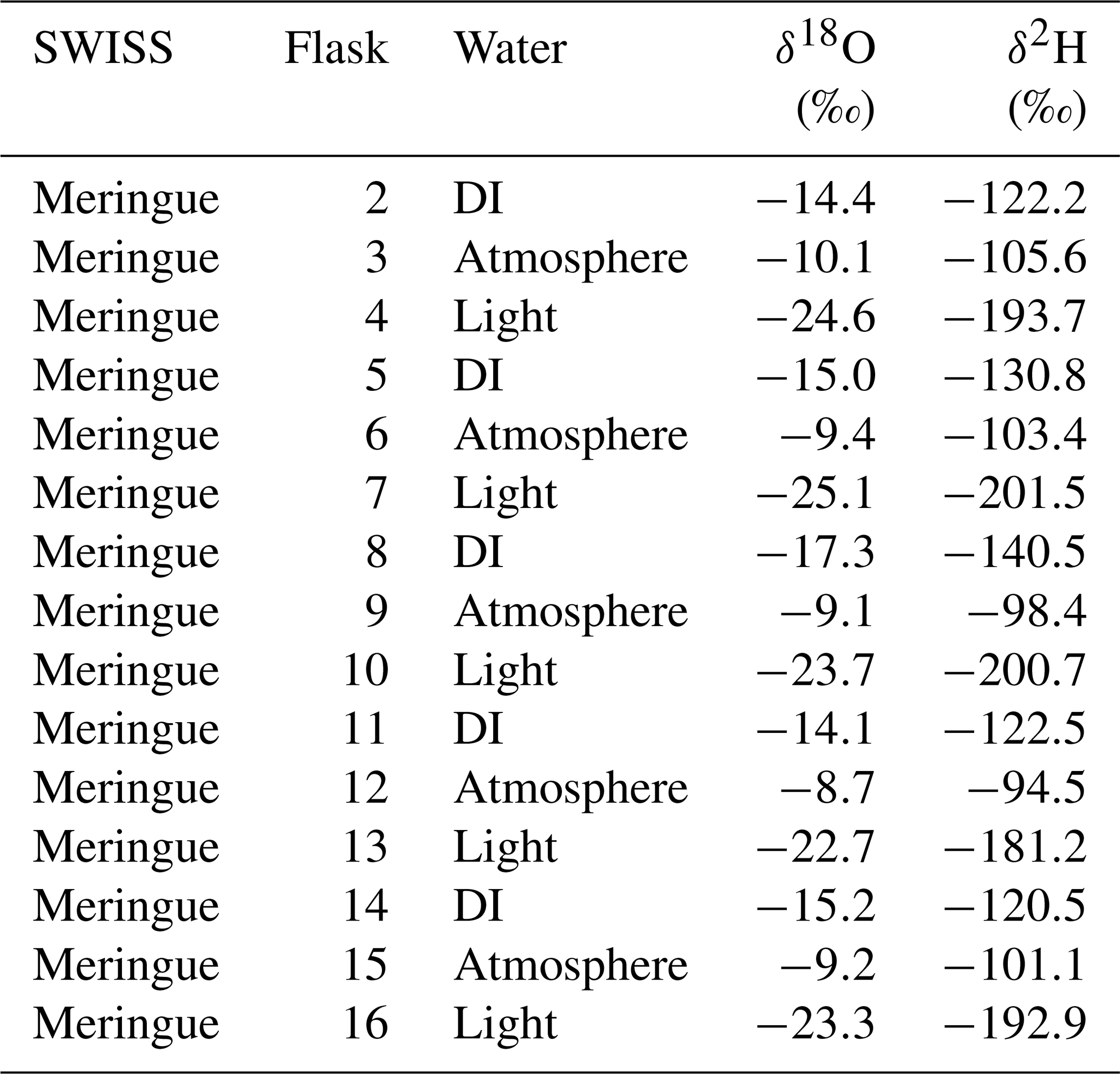
To test whether the automation code and sampling scheme that we developed worked as expected on short, observable timescales, we set up an experiment to simulate field deployment of one SWISS unit (Meringue) near the University of Colorado Boulder. This test applied the automation components and remote power setup described in Sect. 3. During this field-simulation experiment, our goal was to collect three discrete samples each sampling period in order to simulate the collection of water vapor from three soil depths. An important goal of this test was to test whether the sampling scheme introduced any memory effects between samples. We followed the sampling protocol described in Fig. 2 and Table 1.

The day before the experiment began, all flasks were flushed with dry air as described in Sect. 4.1.2. Over the course of 25 h, all 15 flasks were filled with three different vapors according to a set schedule, as would be done in the field. Two of the vapors were created by immersing the water-vapor-permeable probes in the light water and intermediate water as described in Sect. 4.1.3. The third was water vapor from the ambient atmosphere. All three vapors were sampled using vapor-permeable probes constructed identically to those deployed in the field. For this experiment, we filled three flasks per cycle with each one of the waters (e.g., flask 2 was light water, flask 3 was intermediate water, and flask 4 was atmosphere). The choice to sample atmosphere alongside two waters reflects our second goal of this test, which was to demonstrate that sampled water vapor isotope values do not drift towards atmospheric values (Magh et al., 2022).

Following the sampling schedule, we stored the SWISS unit in a simulated field setting for 7 d. At the end of the 7 d, we measured the flasks. For flasks that had a high water vapor mole fraction (i.e., light and intermediate water vapor samples), we used the dry-air carrier-gas-sample introduction method. For flasks that had a low water vapor mole fraction (i.e., atmosphere, ∼15 000 ppm), we used the dead-end pull sample introduction method.

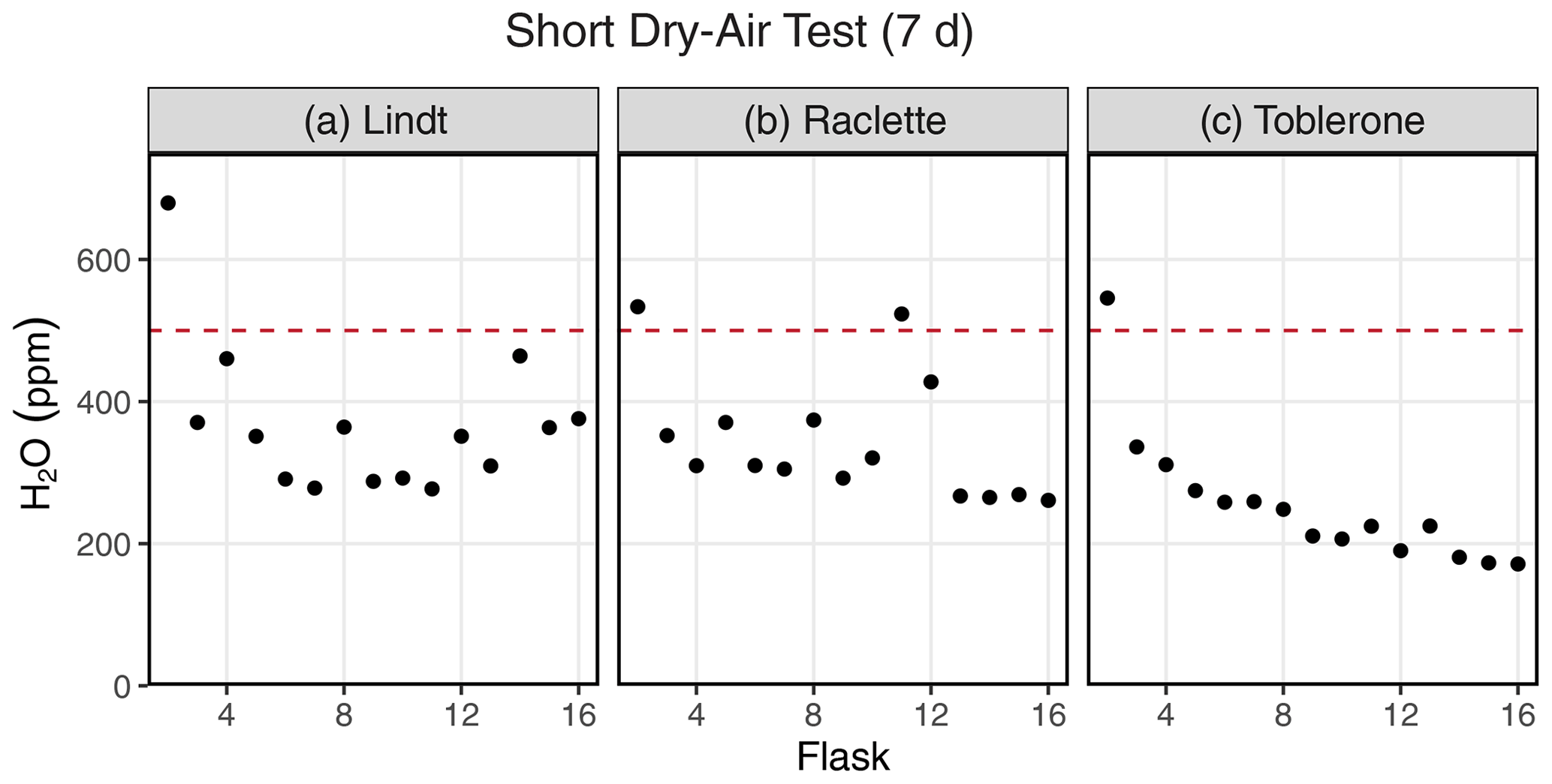
Figure 3 Results of a dry-air test from three different SWISS units: (a) Lindt, (b) Raclette, and (c) Toblerone. The majority of the flasks maintain a water vapor mixing ratio of less than 500 ppm.

To create average values for each flask, we followed the same averaging protocol described in Sect. 4.1.3. We used Eqs. (2a) and (2b) from Rothfuss et al. (2013) to convert from water vapor to liquid values. Then, using secondary and tertiary standards, data were corrected into the VSMOW/SLAP isotope scale. Finally, the SWISS unit offset correction (detailed below in Sect. 6.1.2) was applied.

4.3 Example field deployment: 1-month period

We deployed one SWISS unit each to the three field sites described in summer 2022. Before deployment, all SWISS units were flushed with dry air following the protocol outlined in Sect. 4.1.2. Flasks were flushed with dry air 1–3 d prior to field deployment. At each site, we sampled at three depths (25, 50, and 75 cm) on each sampling day, following the protocol described in Fig. 2 and Table 1. We sampled soil water from all three depths every 5 d (protocol length of 25 d total). At Oglala National Grassland, NE, samples were taken every 5 d from 26 June to 14 July 2022. At the Briggsdale, CO, site samples were taken every 5 d between 17 July and 6 August 2022. At the Seibert, CO, site, samples were collected every 5 d between 19 June and 4 July 2022. At the end of a 28 d period, the SWISS units were returned to the lab and measured. SWISS units were measured within 5 d of returning from the field. The maximum number of days that a flask held sample water vapor during these deployments was 32 d. The measurement protocol and data averaging protocol follow the procedures described in Sect. 4.1.3. The data correction scheme follows the process outlined in Sect. 4.2.2.

5 Results

5.1 QA/QC results

5.1.1 Dry-air test

Figure 3 shows the results of a 7 d dry-air test for three SWISS units (marked by the unit name) (Table S3). For all three SWISS units, at least 13 of the 15 flasks maintained a water vapor mole fraction value of less than 500 ppm over the 7 d period. In two of the three SWISS units (Lindt and Raclette), the water vapor mole fraction for flasks was randomly distributed around approximately 350 ppm. In Toblerone, there was a systematic decrease in the water vapor mole fraction from flask 2 through flask 16, matching the order in which the flasks were filled with dry air initially. In all three SWISS units, flask 2 had the highest water vapor mole fraction of all the flasks. Figure S2 shows the results of successive dry-air tests on the SWISS unit Toblerone where Swagelok fittings were tightened between tests. Between the two tests, there was a significant decrease in the measured water vapor mole fraction for many flasks, but this was particularly noted for flasks 10 and 11 as a result of tightening the fittings.

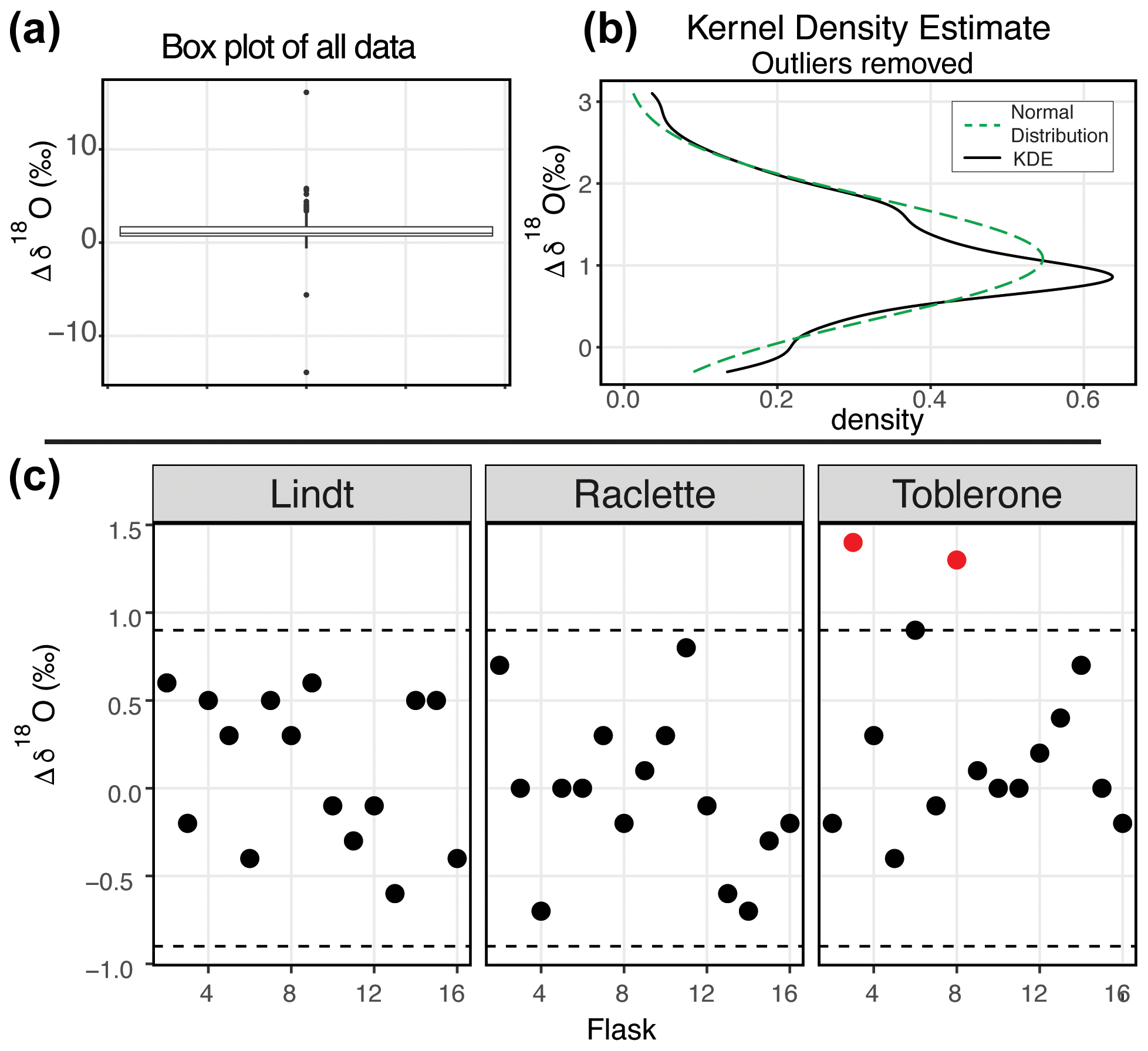
Figure 4 δ¹⁸O results of the water vapor tests. (a) Box plot of the difference between the starting δ¹⁸O value and the final δ¹⁸O value of all 164 flasks. (b) After removing the outliers from the dataset, the kernel density estimate (black line) and the normal distribution calculated from the dataset (dashed green) are shown. (c) After applying the offset correction of 1.0 ‰, the difference between the starting δ¹⁸O value and the final δ¹⁸O value for three SWISS units from the August 2022 session are shown. An uncertainty of ±0.9 ‰ is marked with a dashed line, and data points that fall outside that uncertainty are colored red.

5.1.2 Water vapor test

Figure 4 shows the δ¹⁸O results of 11 water vapor tests performed using six different SWISS units. Ideally, we expect a normal distribution centered about 0 within the uncertainty limits of the water vapor probes (Oerter et al., 2016). For δ¹⁸O, the mean difference between the start and end values for the flasks is 1.1 ‰ with a standard deviation of 0.72 ‰ (outliers removed). There is a consistent positive offset, with a few clear outliers (Fig. 4a). We do not observe a consistent difference between water vapor sample introduction methods (Fig. S3). After removing outliers ($<Q_{\mathrm{1}}-\mathrm{1.5}\cdot \mathrm{IQR}$ or $>Q_{\mathrm{3}}+\mathrm{1.5}\cdot \mathrm{IQR}$, n=15, where IQR represents the interquartile range) from the dataset, we compared the kernel density estimate shape to a normal distribution calculated from the mean and standard deviation of the dataset to assess dataset normality (Fig. 4b). A normal distribution slightly overestimates the center of the data but captures the overall shape fairly well. Therefore, we used the median offset (1.0 ‰) to correct our water vapor isotope values and the IQR of the dataset (outliers removed) to estimate uncertainty of the SWISS as ±0.9 ‰. In Fig. 5c, for simplicity, we just present the results from 45 flasks (three SWISS units), with the 1.0 ‰ offset correction applied. After correction, data are randomly distributed about zero and are within the uncertainty range of ±0.9 ‰ (Table S4).

Figure 5 shows the δ²H results of 11 water vapor tests. For δ²H, the mean difference between the start and end values is 2.63 ‰ with a standard deviation of 2.85 ‰ (outliers removed). Similar to δ¹⁸O, we expected a normal distribution of differences centered around zero. As with δ¹⁸O, there was a consistent positive offset with some outliers (i.e., $<Q_{\mathrm{1}}-\mathrm{1.5}\cdot \mathrm{IQR}$ or $>Q_{\mathrm{3}}+\mathrm{1.5}\cdot \mathrm{IQR}$) (Fig. 5a). After removing outliers (n=26) from the dataset, we compared the kernel density estimate to a normal distribution calculated from the mean and standard deviation of the dataset to assess dataset normality (Fig. 5b). As with δ¹⁸O, the center of the dataset is overestimated by the mean, but the overall peak shape is roughly captured. Therefore, we use the median value of 2.3 ‰ as an offset correction and estimate uncertainty at ±3.7 ‰ for δ²H from the interquartile range. In Fig. 5c, we present the results from 45 flasks (three SWISS units), with the 2.3 ‰ offset correction applied. Data are randomly distributed about zero and are within the uncertainty range of ±3.7 ‰ (Table S4).

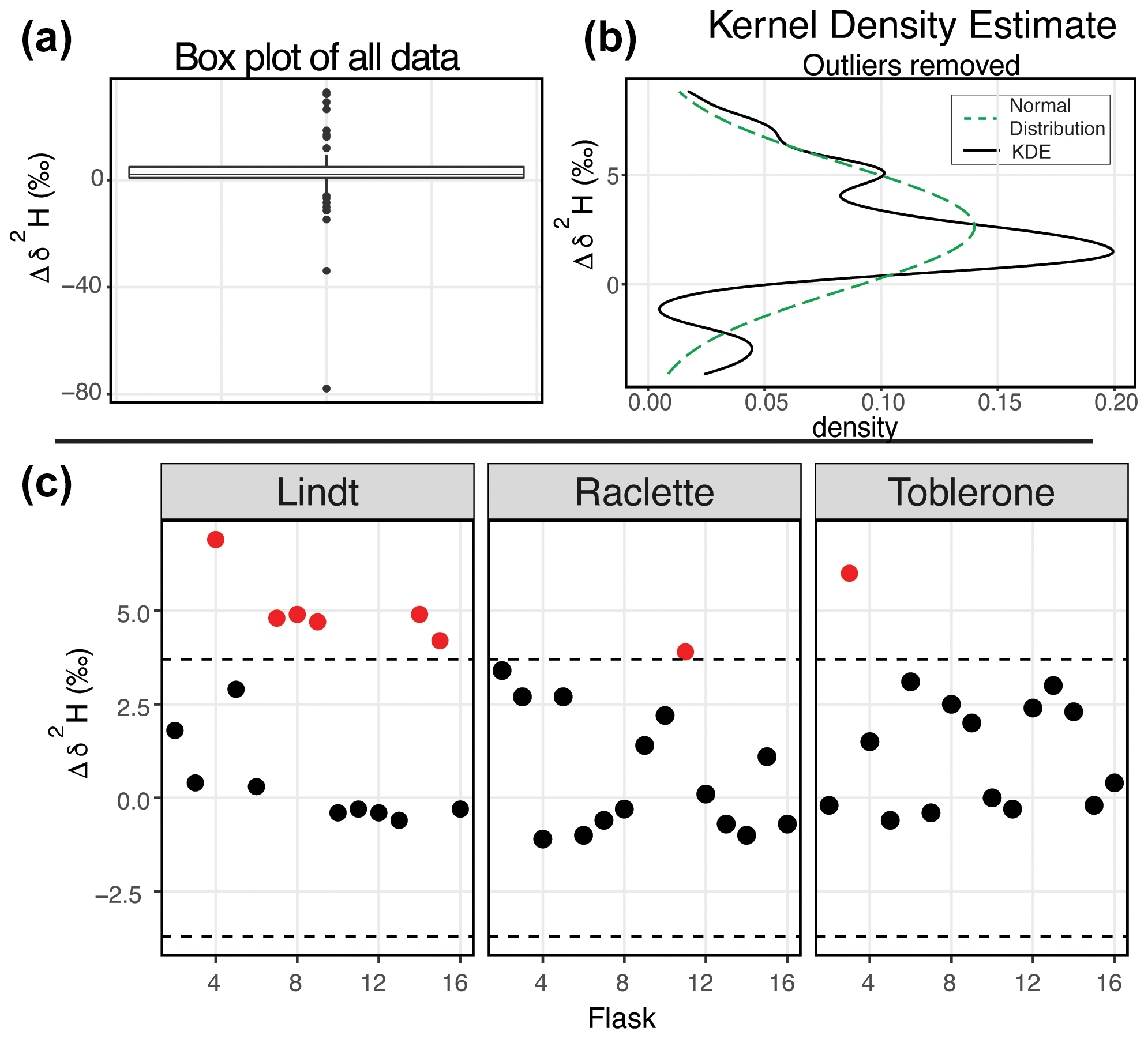
Figure 5 δ²H results of the water vapor tests (a) Box plot of the difference between the starting δ²H value and the final δ²H value of all 164 flasks. (b) After removing the outliers from the dataset, the kernel density estimate (black line) and the normal distribution calculated from the dataset (dashed green) are shown. (c) The difference between the starting δ²H value and the final δ²H value for three SWISS units from the August 2022 session are shown after applying the offset correction of 2.3 ‰. An uncertainty of ±3.7 ‰ is marked with a dashed line, and data points that fall outside that uncertainty are colored red.

When we compared the results in Figs. 4c and 5c, we found that flasks that performed adequately for δ¹⁸O did not always perform adequately for δ²H. The results from the SWISS unit Lindt display this behavior particularly well. Less commonly, some flasks that were within the uncertainty of the system for δ²H were not within the uncertainty of the system for δ¹⁸O, like flask 8 in the SWISS unit Toblerone (Figs. 4c, 5c). In a dual-isotope plot, there is a strong positive correlation between δ²H and δ¹⁸O with a slope of 3.14 and an R² value of 0.62 (Fig. S4).

5.2 Field suitability test results

5.2.1 Dry-air test

Figure 6a shows the result of placing three different SWISS units that were flushed with dry air out into the field for 34–52 d (Table S3). This timescale (4–6 weeks) is similar to most field deployments. At the timescale of 34–43 d, 13 of the 15 flasks typically maintained a water vapor mole fraction of less than 1000 ppm. Over the 52 d, seven flasks maintained a water vapor mole fraction of less than 1000 ppm, whereas the remaining eight had a water vapor mole fraction of between 1000 and 2500 ppm.

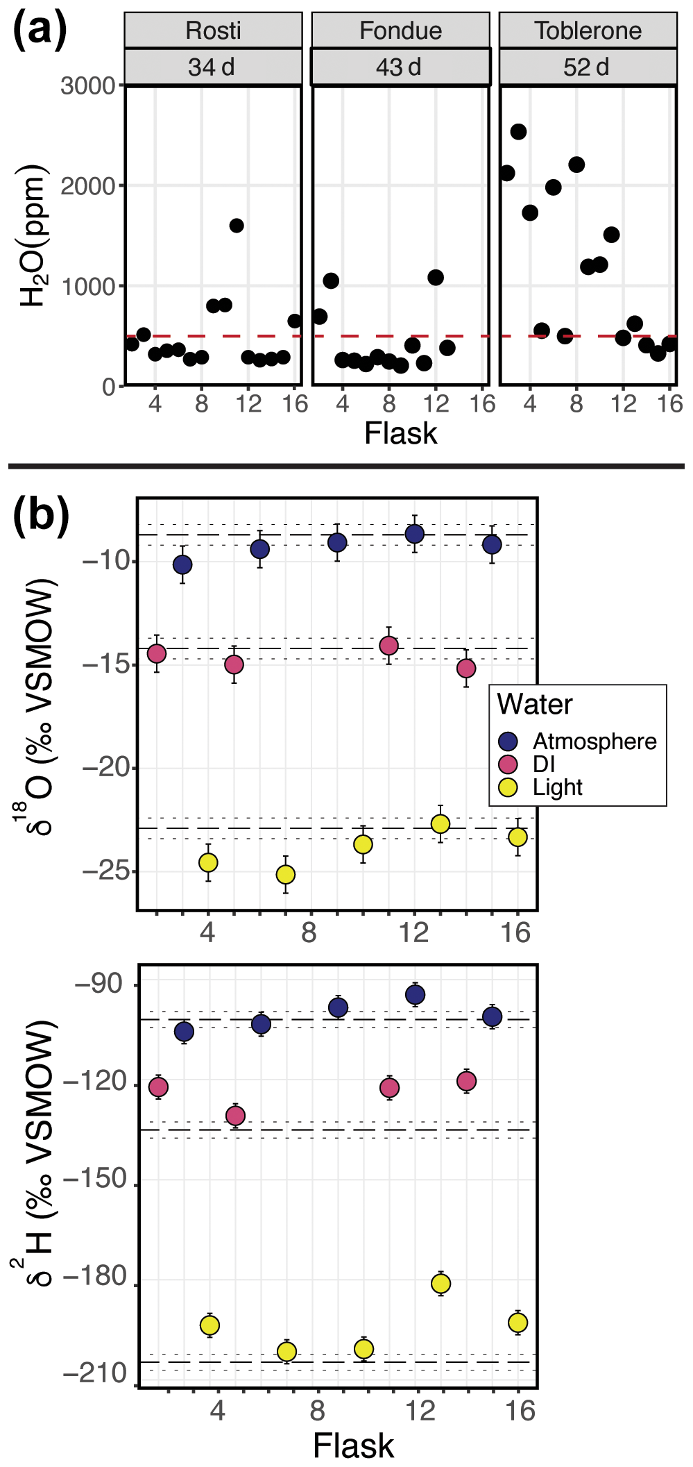
Figure 6 (a) Results from three different field-based long dry-air tests. (b) Results from the automation field suitability tests using the SWISS unit named Meringue. Flasks that sampled atmosphere are shown in blue, flasks that sampled deionized water (DI) are shown in pink, and flasks that sampled the light water are shown in yellow. In panel (b), the top plot shows the δ¹⁸O results and the bottom plot shows the δ²H results.

5.2.2 Automation test

Figure 6b shows the results of using the automation code to collect and store water vapor of known composition for 7 d (Table 2). In both plots, the known values of the water are shown as a dashed line. Uncertainty on those measurements is estimated at ±0.5 ‰ and ±2.4 ‰ for δ¹⁸O and δ²H, respectively (Oerter et al., 2016), shown as the dotted lines. We estimated the isotope value of the atmosphere at the time of sampling with the water vapor mole fraction, δ¹⁸O, and δ²H data from the CRDS in the lab. The isotope value, which was corrected as described in Sect. 4.2.2, of each flask is shown, with the uncertainty associated with the SWISS units, estimated to be ±0.9 ‰ and ±3.7 ‰ for δ¹⁸O and δ²H, respectively.

Table 2 Results of the automation test.

Seven of the nine flasks filled with flash-evaporated water vapor overlap within uncertainty of the known δ¹⁸O value for those standards (top plot in Fig. 6b), and four of the five flasks filled with atmospheric vapor overlap within uncertainty of our estimated δ¹⁸O value. Flasks that fall outside of the bounds of uncertainty have lower δ¹⁸O values than the expected value. For δ²H (bottom plot in Fig. 6b), only three of the nine flasks filled with flash-evaporated water vapor overlap within uncertainty of the known value of those standards, while four of the five flasks filled with atmospheric vapor overlap within uncertainty of the estimated δ²H value. Flasks that fall outside of the bounds of uncertainty have higher δ²H values than the expected value.

5.3 Example field-deployment results

Figure 7 shows the results from three field deployments in Oglala National Grassland, NE; Briggsdale, CO; and Seibert, CO (Table 3).

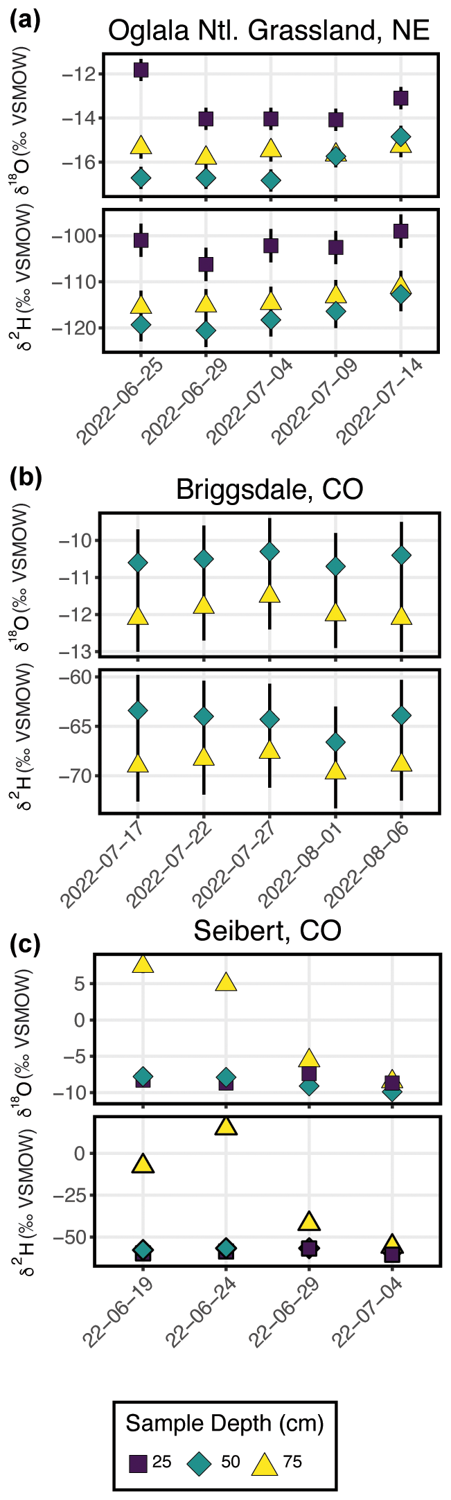
Figure 7 Results from all three field deployments to (a) Oglala National Grassland, NE; (b) Briggsdale, CO; and (c) Seibert, CO. Note that the y-axis scale for all three plots is different.

Table 3 Results from the three field deployments of SWISS.

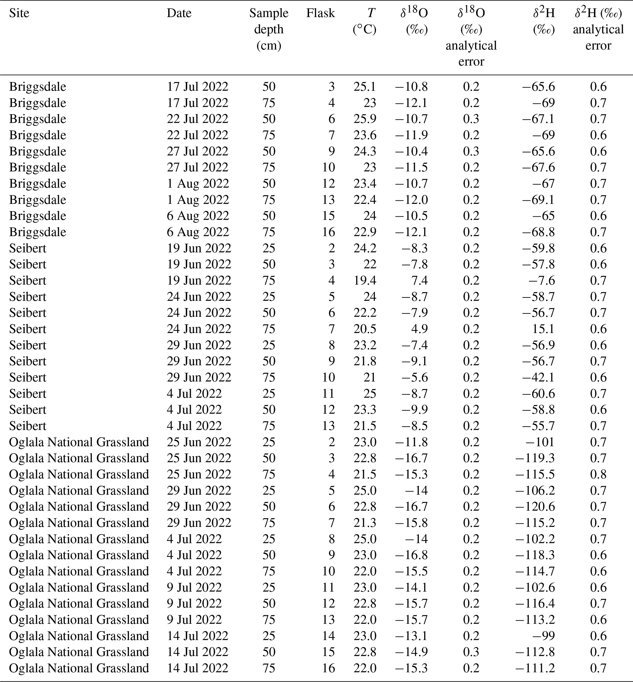
There are 15 samples from Oglala National Grassland (Fig. 7a, Table 3): 5 from 25 m depth, 5 from 50 cm depth, and 5 from 75 cm depth. Four of the five samples from 25 cm overlap within uncertainty with respect to the δ¹⁸O value, and all five samples overlap with uncertainty with respect to the δ²H value. There is a significant decrease in the δ¹⁸O value at 25 cm between 25 and 29 June 2022. There is no similar shift in the δ²H value over the same time period. The first three samples from 50 cm overlap with respect to both the δ¹⁸O and δ²H values, and the final two samples then shift to higher isotope values. Similar to the samples from 50 cm, there is a trend towards higher δ²H values for the last three samples. All five samples from 75 cm overlap with respect to the δ¹⁸O and δ²H values. On a dual-isotope plot, data from 50 and 75 cm cluster together at lower values, whereas the δ¹⁸O and δ²H values from 25 cm are higher (Figs. 7a, 8a). All of the data overlap within uncertainty with the global meteoric water line (GMWL), except for the 25 cm depth sample from 25 June 2022 (Fig. 8a). The calculated d-excess values are all within an uncertainty of 10 ‰ (±2.6 ‰) and of each other between 29 June and 14 July 2022 (Fig. 8b), except for the 25 cm depth sample from 25 June 2022, which has a d-excess value of −6.6 ‰, typically consistent with evaporative enrichment of soil water at that depth and time.

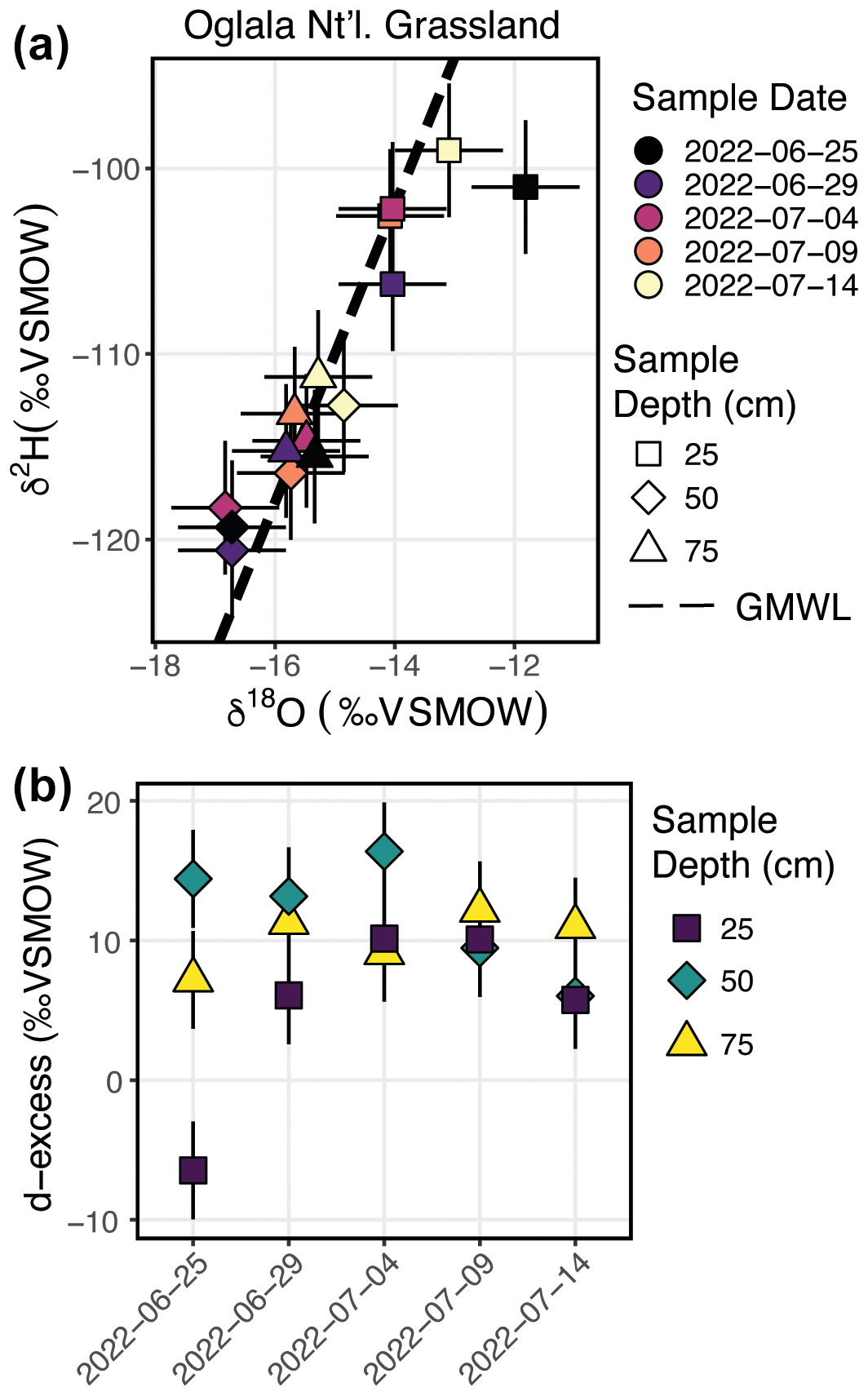
Figure 8 Results from the Oglala National Grassland, NE, field site. Panel (a) shows δ²H vs. δ¹⁸O, where the dashed line is the global meteoric water line. The shapes for the different depths sampled match Fig. 7, and the color of the points is the date on which the soil water was sampled Panel (b) presents a plot of d-excess; note that both the color and shape match Fig. 7.

There are 10 samples from Briggsdale, CO (Fig. 7b, Table 3): 5 samples each from vapor probes buried at 50 and 75 cm depth. Data from 25 cm at Briggsdale, CO, were excluded because the water vapor mole fractions from all of the flasks were extremely low (<13 000 ppm). We excluded these data because these samples are associated with a very dry soil (volumetric water content < 0.05), and it is not clear how much sampling gas (N₂) is injected into the soil using the vapor-permeable tubing under very dry conditions (Quade et al., 2019) and, therefore, how representative these isotope data are of soil water. Moreover, there are large linearity effects below 13 000 ppm on a Picarro L2130-i, and it is challenging to correct these data if they were measured using the dry-air carrier-gas-sample introduction method. While all samples overlap within uncertainty for both δ¹⁸O and δ²H values, the absolute values of samples from 50 cm are consistently offset to higher values for both δ¹⁸O and δ²H compared with samples from 75 cm.

There are 12 samples from Seibert, CO (Fig. 7c, Table 3): 4 from each respective sampling depth (25, 50, and 75 cm). At 25 cm depth, δ¹⁸O values of three of the four samples overlap within uncertainty, whereas the 25 cm sample from 29 June 2022 has a higher δ¹⁸O value than the other three samples. At 25 cm depth, δ²H values overlap within uncertainty for all four samples. At 50 cm depth, there is a steady decrease in the δ¹⁸O value over the sampling period, while δ²H values for all four samples remain steady and overlap within uncertainty. At 75 cm depth, samples have a very large range of δ¹⁸O values between −8.5 ‰ and 7.4 ‰, and δ²H values range between −55.7 ‰ and 15.1 ‰.

6 Discussion

6.1 QA/QC and field suitability tests

6.1.1 Dry-air tests

In Colorado, where these tests were completed, the ambient atmosphere during the summertime typically sits at a water vapor mole fraction of between 10 000 and 20 000 ppm, and the water vapor mole fraction can drop as low as 4000 ppm in winter. If the flasks had been slowly equilibrating with the atmosphere, the flasks would have drifted to much higher water vapor molar fractions. If the flasks did not drift towards higher water vapor mole fractions, we felt confident that the flasks were resistant to atmospheric intrusion after they had been flushed with dry air. We chose a timescale of 7 d for the dry-air tests, as we found that, in a low-humidity environment, 7 d was enough time to meaningfully observe leaks while also being short enough to work through the QA/QC process efficiently. For example, results of two sequential dry-air tests on the SWISS unit Toblerone (Fig. S2) show that it is possible to drastically reduce leaks that allow ambient water vapor to intrude into the flasks by tightening and/or replacing problematic fittings (both those attached to the glass flasks and those on the Valco valve) and, in some rare cases, the glass flask itself. During the final 7 d dry-air tests, most flasks maintained a water vapor mole fraction of less than 400 ppm, and all flasks maintained a water vapor mole fraction of less than 700 ppm (Fig. 3).

Across all of the SWISS units, there is a bias towards a higher water vapor mole fraction for the first flask that is measured (port 1 on every valve is the flask bypass loop, so the first flask is flask 2), which suggests a methodological source of higher water vapor concentration rather than Swagelok fitting tightness problems. There are two potential sources for this issue. First, it is possible that not all of the atmospheric water vapor was flushed from the line that connects to the CRDS prior to the start of the measurements; however, by the time the second flask is measured, the lines between the SWISS and CRDS have been sufficiently flushed, thereby creating bias in the first flask measured. This hypothesis could be tested by flushing all of the gas lines with dry air to progressively lower water vapor mixing ratios prior to measuring any flasks to see what minimum ratio is required to eliminate this bias. Lab protocols could then be adjusted to flush all gas lines to this level. Similarly, it is possible that, during the filling phase, not all of the atmospheric vapor has been flushed out of the Drierite system before starting the fill process. This hypothesis is supported by the systematic decrease in the water vapor mole fraction across flasks in the Toblerone unit (Fig. 3c). As a result of these biases, we now flush the Drierite for at minimum 30 min prior to the start of the experiment.

In addition to testing the leakiness, the dry-air test also provided a useful baseline from which to test building materials. For example, in Fig. S5, we show the results of sequential 7 and 27 d dry-air tests in which we replaced stainless-steel tubing and fittings with PTFE Swagelok fittings with $\mathrm{1}/\mathrm{8}$ in. PTFE tubing. We thought that PTFE fittings would be advantageous because they are much easier to install and are significantly lighter, which would be helpful when there are weight constraints. However, based on the very limited testing that we did, PTFE fittings and tubing may be sufficient to store water for up to a single week; however, on longer timescales (e.g., 27 d), we observed greater exchange and leaking than with the stainless-steel fittings. We encourage any future user using this modification to rigorously test these fittings on a timescale appropriate for their application.

6.1.2 Water vapor tests

Our initial goal with the water vapor tests was to test whether the measured water vapor isotope values at the end of the 2-week holding period were normally distributed about zero within the uncertainty limits of the water vapor probes (Oerter et al., 2016). This was a reasonable goal given the similarities in probe setup and the plumbing design between the SWISS and the IsoWagon system (Oerter et al., 2016). However, the most salient result of the water vapor tests is that there is a consistent positive offset between the input isotope values and the isotope values measured at the end of the 2-week experiments (Figs. 4b, 5b). The positive offset in both the δ¹⁸O and δ²H values is consistent across 11 different tests, using six different SWISS and three different input water isotope values. If there was alteration of the original values due to leaky flasks, we might expect the δ¹⁸O and δ²H values to converge on the δ¹⁸O and δ²H value of the atmosphere. For example, we might expect water vapor from the light-water test to have the most significant change in isotope value, towards that of the ambient atmosphere. Instead, the consistency across >135 flasks, different starting water vapor isotope values, sample introduction methods, and multiple analytical sessions suggests that this difference is a function of the storage and measurement process. In particular, the normality of the distribution suggests that, whatever the origin of the offset is, there is a systematic bias that we can reliably correct for.

Offset correction

To correct our data for this offset, we chose to use the median value as an offset correction, rather than the mean of the normal distribution, as the median is not biased by major outlier isotope values that reflect abnormal values that go beyond analytical noise, such as a slow but major leak that changes the values far beyond the basic offset seen in the dataset. The calculated average offset is 1.0 ‰ and 2.6 ‰ for δ¹⁸O and δ²H, respectively. After applying these values as an offset correction to the data, most flasks also fall within the uncertainty of the water-vapor-permeable probes (δ¹⁸O = ±0.5 ‰ and δ²H = ±2.4 ‰; Oerter et al., 2016), and the values are distributed about zero (Figs. 4c, 5c). However, the uncertainty of the SWISS system is higher than that of the probes alone. Based on the results of the water vapor tests, we estimate the uncertainty of the SWISS to be ±0.9 ‰ and ±3.7 ‰ for δ¹⁸O and δ²H, respectively, using the IQR of the water vapor test results after removing outliers from the dataset. We prefer the IQR over the calculated standard deviation of the normal distribution because the IQR is not biased by outlier values. This level of uncertainty is large relative to other methods but is sufficient for many critical zone applications, given the magnitude of seasonal variability in the top ∼50 cm of a soil profile that can be observed in natural systems (e.g., Oerter and Bowen, 2017; Quade et al., 2019). We also expect that uncertainties will decrease with future lab-based or near-research-facility testing and by comparing the SWISS against other soil water extraction methods.

The relationship between δ²H values and δ¹⁸O values in a dual-isotope plot provides insight into the mechanism driving the offset. Without an offset correction applied, the slope of the relationship between δ²H and δ¹⁸O is 3.14 (R²=0.62) (Fig. S4). This slope is only slightly higher than evaporation under pure diffusion (Gonfiantini et al., 2018). This suggests that the offset is likely driven by diffusion and will likely vary according to the climate of the lab. For example, in a dry climate like Colorado, the water vapor concentration in the flask is significantly higher than the atmosphere, creating a larger diffusive gradient potential than for a lab in a more humid climate. Therefore, we strongly encourage future users to test their SWISS under climate conditions similar to those of their intended applications. Furthermore, we encourage users who might use the SWISS as part of a tracer study that uses labeled heavy water to test the SWISS with labeled waters prior to their field experiments to verify reliability.

Comparing sample introduction methods

Figure S6 shows a kernel density estimate plot of the results from two water vapor test sessions, with the offset correction applied. During the March 2022 session, flasks were measured using the dead-end pull sample introduction method; during the August 2022 session, flasks were measured using the dry-air carrier-gas-sample introduction method. There is no significant difference in the measured difference between the two sample introduction methods. That said, we prefer the dry-air carrier-gas method, as it is far simpler to control the water vapor mixing ratio and optimize the concentration to be around 25 000 ppm, which is the concentration at which the Picarro L2130-i is most reliable. The dry-air carrier-gas method also makes it easier to control for and monitor for condensation in the stainless-steel tubing and vapor-impermeable tubing, which can bias a measurement.

6.1.3 Field suitability tests

The long dry-air tests in the field are a useful complement to the shorter in-lab tests because they test the reliability of the system at field-deployment timescales. It is clear from the 34 and 43 d tests that the flasks are reasonably resistant to leaks on the timescale of a normal 4- to 6-week deployment (Fig. 6a). These tests also give us confidence that flasks filled later in the sampling sequence do not take on an atmospheric signal prior to sampling. There are a few possibilities to explain the poorer performance of the Toblerone SWISS unit during the 52 d test (Fig. 6a). The first is that there is a real threshold past which SWISS units are no longer able to retain samples. However, this explanation would suggest that there should be a gradual decrease in performance across the three tests, which we do not observe. The alternative explanation is that the poor performance is a result of inter-unit variability. The 52 d test was the first long-term test and was performed in August 2021. In August 2021, we were continuing to build new SWISS units and continuing to learn from each successive round of QA/QC; thus, it seems plausible that there were unidentified problems with the SWISS unit Toblerone that were solved before the water vapor tests in August 2022.

In Fig. 6b, the data show that the flasks preserved the δ¹⁸O value of both flash-evaporated and atmospheric water vapor over a 7 d period. One flask was removed from the dataset (flask 8), because there was visible condensation in the clear impermeable tubing during the measurement phase, with an increase of >5 ‰ for δ¹⁸O during the measurement period. The condensation appeared as small (<1 mm) bubbles of water all along the impermeable tubing, but the bubbles were concentrated near the connection between the SWISS and the impermeable tubing. Notably, the two flasks whose δ¹⁸O values do not overlap within uncertainty are more negative than expected, rather than drifting towards atmospheric values or values expected from diffusive fractionation. In contrast to the δ¹⁸O values, only three flasks filled with flash-evaporated water vapor overlap within uncertainty of the known δ²H values, while four of the five flasks overlap within uncertainty of the estimated atmosphere isotope value. The flasks tend to drift towards the value of the atmosphere, but they retain the overall data pattern from the oxygen isotope values.

The relatively high failure rate of this “mock” field test was somewhat surprising given the results of the water vapor tests done in the laboratory. Going into the test, we suspected that flasks 6 and 8 were slightly leaky based on previous water vapor tests; these were flasks that previously performed poorly but did not “fail” during the water vapor test. Once we collected the data, we compared the data for flasks 6 and 8 to other flasks in the sequence. During the measurement of flask 8, we observed condensation in the sample introduction lines, and, as the isotope values were so different relative to other flasks, we felt confident in our exclusion of flask 8. Flask 6 had δ¹⁸O and δ²H values similar to others from the same sampling source and seemed to fall within the pattern as expected; therefore, we chose to keep this data point in the dataset.

We hypothesize that one major problem with the mock field test dataset was the creation of condensation in the sampling lines, as others have experienced in their setups (e.g., Quade et al., 2019; Kühnhammer et al., 2022). Of particular interest are the flasks that had a lower than expected δ¹⁸O value (flasks 4 and 9). It is possible that those samples were also affected by condensation; however, in contrast to flask 8, which was excluded because of condensation during measurement, we think that these samples may have been altered because of condensation at the sampling stage. During condensation, we expect that ¹⁸O will preferentially enter the liquid phase and that the water vapor that enters the flask will have a lower than expected δ¹⁸O value. The unique advantage of the SWISS is that it can operate independently but with that comes the trade-off that we cannot currently observe condensation in the lines during sample collection. To prevent condensation from forming, other users have warmed the impermeable tubing between the probes and the Picarro instrument. The mock field test data suggest that it may be worthwhile in many situations to warm the transfer tubing, but this should be done in a way that does not alter the thermal structure of the soil and that can operate safely and independently in remote settings.

6.1.4 Lessons learned and recommendations from the QA/QC and field suitability tests

Our QA/QC process was a relatively efficient way to test the soundness of the SWISS units. Through the QA/QC process, we were able to identify problems with units and appropriately address these issues before deploying units to the field. We strongly recommend that any user deploying a SWISS unit to the field undertake the same, or similar, QA/QC process.

The dry-air test is a time-efficient and low-cost method for identifying flasks that are leaky and will not preserve the sampled water vapor isotope values. During the building stage, it is useful to identify fittings that need to be tightened or flasks that need to be replaced; therefore, we recommend these tests as a required pre-deployment step for future SWISS units. We found that it was most time and energy efficient to move onto the next level of QA/QC once 13 out of 15 flasks of a SWISS unit had passed the dry-air test, as the remaining two flasks still frequently had relatively low water vapor mole fractions (i.e., 500–700 ppm), and we could sufficiently tighten the fittings prior to the start of the water vapor tests for them to be successful. The dry-air test is a low time and expense burden that can also be used to monitor SWISS units for normal wear and tear (e.g., a flask that cracked during transport) during deployment periods. Therefore, to ensure that SWISS units continue to operate as expected, we also recommend that dry-air tests be done between field deployments on every SWISS unit. Lastly, we note that the dry-air test could be modified based on available equipment (for example, if an instrument is available to measure trace atmospheric gases, that could be used instead).

Based on the results of the long dry-air field test, we recommend that the water vapor storage time does not exceed 40 d for reliable results or that the user undertake multiple dry-air tests with either lower-concentration benchmarks or a longer duration if deployments may exceed 40 d.

Overall, the quality control and quality assurance as well as the field suitability tests demonstrate that the SWISS units can retain the isotope values of water vapor collected using water-vapor-permeable probes. Like many other systems that measure dual isotopes (i.e., δ¹⁸O and δ²H), each system must be evaluated separately. In general, we interpret oxygen isotope data with a higher degree of confidence than hydrogen isotope data. As the automation test revealed, however, even when the absolute δ²H value is not correct, the general pattern can reveal information about soil water dynamics.

Finally, we opted to use a large flask volume because we hypothesize that it allows us to measure a sample for long enough on a CRDS that we get reliable data, without interacting with vapor bound to the flask walls. The drawback of this, however, is that we must sample soil water vapor for a relatively long period of time (45 min). In Fig. S7, we show that the sampling regime, and particularly the length of time that we pump dry air through the tubing, does not significantly alter the soil moisture content of the soil. Additionally, we demonstrate that the sampling regime that we use does not introduce significant memory effects.

6.2 Field deployments

In Fig. 7, we show the results of three field deployments completed during summer 2022 (Table 3). At the Oglala National Grassland site, we used the SWISS unit named Lindt to collect samples. During the August 2022 water vapor test on Lindt, all δ¹⁸O values fall within the uncertainty of the system, and 9 of the 15 δ²H values fall within the uncertainty of the system. Therefore, we interpret the δ¹⁸O values with greater confidence and the δ²H values with lower confidence (Figs. 4c, 5c). We note that the δ¹⁸O and δ²H values broadly follow the same trends and fall on the global meteoric water line (Figs. 7, 8a). In general, soil water from 25 cm had higher δ¹⁸O and δ²H values than soil water from both 50 and 75 cm (Fig. 8a). Given that four of the five samples from 25 cm overlap with the GMWL and have a d-excess that overlaps with 10±2.6 ‰, the soil water from that depth may reflect summer precipitation with higher δ¹⁸O and δ²H values. Soil water from 75 cm had intermediate δ¹⁸O and δ²H values for most of the study period, and soil water from 50 cm depth had the lowest δ¹⁸O and δ²H values for most of the study period, which may reflect a more mean annual or winter precipitation biased value. Based on data available from the National Weather Service (Chadron, NE), there were likely significant precipitation events on 25 June and 8 July 2022 at the field site. There is a significant shift to lower δ¹⁸O values at a sampling depth of 25 cm between 25 and 29 June 2022 as well as a marked increase in the d-excess value (Fig. 8a). We interpret this shift as the infiltration of precipitation with lower δ¹⁸O values, which is supported by a return of d-excess values to ∼10 ‰ (Fig. 8a). The National Weather Service reported 21.33 mm (0.84 in.) of rain at Chadron Municipal Airport, approximately 50 km from the study site, on 8 July 2022, which likely was associated with at least some precipitation at our field site. Following the significant rain event on 8 July 2022, we observe a marked increase in the stable isotope value of water vapor from a sampling depth of 50 cm towards values that are much closer to those at 25 cm depth. These data suggest that soil water isotopes at 50 cm in this silt-loam Aridisol may be fairly sensitive to large individual precipitation events, whereas soil water isotopes remain comparatively uniform at 75 cm. Future work should address how drought conditions, storm size, pore size distribution, and soil clay mineralogy influence the variability in soil water isotopes with depth.

At Briggsdale, CO, we used the SWISS named Raclette to collect soil water vapor samples. Data from 25 cm depth at Briggsdale, CO, were discarded because the water vapor mole fraction was much lower than would be expected given the soil temperature (i.e., <5000 ppm). The gravimetric water concentration (GWC) at that soil depth at the time of sampling was approximately 4 % throughout the sampling period. Future work should include a multiple-method (cryogenic extraction, centrifugation, etc.) comparison of soil water isotopes at low water contents to better understand what these samples might represent and if they are actually representative of soil conditions.

Based on the results of the August 2022 water vapor test done on Raclette in which all flasks fell within the uncertainty of the SWISS system for both δ¹⁸O and δ²H, except for flask 11 (Figs. 4c, 5c), we interpret all data with greater confidence. Flask 11 corresponds to the 25 cm depth sample from 27 July 2022 and had already been culled from the dataset because of its low water vapor mole fraction associated with very dry soil. The soil water δ¹⁸O and δ²H values from a sampling depth of 50 and 75 cm overlap within uncertainty, but the soil water δ¹⁸O and δ²H values from 50 cm are higher than the isotope values from 75 cm. All of the data from each sampling depth group (i.e., 50 and 75 cm) overlap within uncertainty, conforming to the expectation that soil water from these sampling depths should be fairly invariant (e.g., Oerter and Bowen, 2019). There were precipitation events at the study site on 24, 28, and 31 July 2022. It is possible that the slight negative shift in both δ¹⁸O and δ²H on 1 August 2022 reflects the infiltration of precipitation to those depths, but this is not certain given that all of the measurements from within a sampling depth overlap within uncertainty.

At Seibert, CO, we used the SWISS named Toblerone to collect soil water vapor samples. The soil water isotope data from 75 cm depth at this site offer a few useful lessons for future users. The two key observations of the data from 75 cm depth are that the δ¹⁸O and δ²H values are much higher than those from other two sampling depths and that the δ²H and δ¹⁸O values do not move in parallel with each other. While measuring these samples, we observed condensation in the impermeable tubing at the point where the SWISS connects to the impermeable tubing. Additionally, when we heated the stainless-steel tubing that connects the tubing flask and Valco valve, we observed a rapid increase in the water vapor mole fraction (thousands of parts per million over <30 s) that was accompanied by a rise in the stable isotope value. During these measurements, we were rarely able to get a stable isotope value measurement window; instead, the stable isotope value of the vapor increased continually throughout the measurement. It is for these reasons that we feel confident in discarding the stable isotope data from 19 to 29 June 2022. The final measurement from 75 cm depth on 4 July 2022 approaches a reasonable isotope value when compared to isotope values from the other two depths, and that sample had fewer condensation problems during measurement. However, because we have no sequential context for what a reasonable value for this depth is, we discarded that value as well. For that final 75 cm sample, we were more successful because we warmed the entire length the vapor-impermeable tubing as well as the stainless-steel tubing, flask, and Valco valve evenly so that there were no temperature gradients across the vapor path. If the condensation had only been in the impermeable tubing, it would have been much easier to successfully analyze these samples by just closing off the flask and running dry air through the tubing to remove condensation; however, as condensation was also occurring in the stainless-steel tubing between the flask and Valco valve, this was not possible. It remains unclear why condensation was such a significant problem for samples from that depth as opposed to samples from different depths in the same SWISS unit. Future work should include further testing of the SWISS across different water contents and temperatures to better understand why the phenomenon may have occurred.

Based on the results of the August 2022 water vapor test done on Toblerone, we interpret all data from 50 and 25 cm depth with high confidence, except for flask 3, which is the 50 cm sample from 19 June 2022 (Figs. 4c, 5c). Unlike data from the other two field sites, soil water from 25 and 50 cm overlap within uncertainty. There were two precipitation events at the field site during the sampling period on 25 June and 1 July 2022, but both events were quite small (<0.5 mm, CoAgMet). There is no significant influence of the precipitation events on the δ¹⁸O and δ²H values. The >1.0 ‰ increase in the δ¹⁸O values on 29 June 2022 is surprising given that there is not an increase of comparable magnitude in the δ²H value and that the values measured from 4 July 2022 more closely match the δ¹⁸O and δ²H values from the 2 earlier sampling days. There are two potential explanations for these data. First, this shift is a real signal from an evaporation-driven increase in the δ¹⁸O value and the shift back to a lower δ¹⁸O value on 4 July 2022 is due to the infiltration of precipitation, which could also explain the low d-excess value associated with this measurement (Fig. S8). The second possible explanation is that the 25 cm sample from 29 June 2022 is influenced by condensation at the time of sampling. The dew point at the field site on 29 June 2022 significantly decreased compared with the other sampling days to a monthly minimum of 20.6 ^∘C (CoAgMet). It is possible that environmental conditions encouraged the formation of condensation in the impermeable tubing at the time of sampling; if there was residual condensation in the impermeable tubing, it is possible that we were partially sampling a heavier condensed water. There were no obvious signs of condensation during the time of measurement in the lab. These results highlight the utility of having broad contextual environmental data to aid in the interpretation of soil water isotope data.

All together, these three soil water isotope datasets demonstrate two main findings. First, data from these samples show that the differences between field sites are easily resolvable using the SWISS. For example, the oxygen isotopes range from −14.4 ‰ to −16.3 ‰, from −9.9 ‰ to −10.3 ‰, and from −7.4 ‰ to −9.3 ‰ at 50 cm depth for the Oglala, Briggsdale, and Seibert sites, respectively. These differences likely reflect differences in the stable isotope composition of precipitation as well as infiltration and evaporation dynamics. Second, the sample data retrieved from a SWISS are sufficiently precise to be able to meaningfully resolve vertical profile soil water isotope data. For example, at the Oglala National Grassland field site, soil water from 25 cm clearly has higher δ¹⁸O and δ²H values compared with soil water from a depth of 50 and 75 cm.

6.3 Future improvements and future work

One significant SWISS unit hardware improvement that could be made would be to install a heating implement for the flasks. One source of uncertainty in the current system is the potential effect of uneven heating of the flasks prior to measurement, which may create temperature gradients that are large enough to allow for condensation when warm vapor meets a spot slightly colder than dew point. This could be improved in subsequent iterations of the SWISS with the addition of heat tape or blankets that can deliver controlled heat and create consistent temperatures. This improvement would also help limit the amount of manual intervention needed during measurement and could improve the automation of flask measurement. Additionally, finding a way to safely and automatically heat the impermeable tubing that connects the water vapor probes and the SWISS in a way that does not change the inherent thermal structure of the soil and that is safe for unmonitored use would help to prevent the formation of condensation in the field and reduce the uncertainties related to sampling as well as the number of samples that need to be discarded.

We have made a few improvements to the automation system that were not implemented for the data presented in this contribution but that will be a part of future deployments. First, we will track conditions inside the SWISS with a temperature and relative humidity sensor inside the case. Second, we plan to eliminate the power inverter by powering both the Valco valve and mass flow controller with VDC using a step-up power converter. Lastly, we will add an Internet of Things (IoT) cellular router to be able to remotely monitor and control the SWISS units. This would be particularly helpful if (1) there is a sampling day that is unexpectedly cold or when the dew point at the field site is unexpectedly low and we expect condensation to form more readily in the field or (2) there is a precipitation event that we are interested in capturing, because, with the IoT cellular router, we could remotely alter the sampling plan.

While the improvements and additional testing that we have done to the SWISS in this contribution represent a significant step forward, additional work should be done to make the system more useable by the ecohydrology community. We have rigorously tested the SWISS in the lab and have also demonstrated a few ways in which the SWISS can fail in field settings. A full comparison of how soil water isotope data collected using a SWISS compared with other in situ (both vapor probes and lysimeter) and destructive sampling methods would shed more light on the accuracy and precision of our system as well as on the applicability of our lab-based experiments to the field. These experiments should be carefully designed considering the soil grain size, soil water content, expected isotope values, and climate. Additionally, we plan to test the SWISS unit resilience during air travel so that these units can be used at field sites that are not within driving distance of a research facility.

7 Conclusions

We presented the evolution of the Soil Water Isotope Storage System (SWISS) from a prototype to a fully built-out and tested system. We also presented a quality control and quality assurance procedure that we strongly recommend future users undertake to ensure the reliable storage of soil water vapor over long time periods (up to 40 d). In addition, these quality control and quality assurance tests shed light on the accuracy and precision of the SWISS. After applying an offset correction, we determined the precision of the SWISS to be ±0.9 ‰ and ±3.7 ‰ for δ¹⁸O and δ²H, respectively. In a field setting, flasks reliably resist atmospheric intrusion. Additionally, the proposed sampling schema does not introduce significant memory effects. Lastly, we demonstrated that the current precision of the SWISS still allows us to distinguish between field sites and between soil water dynamics within a single soil column. Taken as a whole, these data show that the SWISS can be used as a tool to answer many emerging ecohydrological questions and that it will enhance researchers' ability to collect soil water isotope datasets from more remote and traditionally understudied field sites.